Numerical Simulations of Incompressible Flows Around a Rotating Circular Cylinder with Convective Heat Transfer Using the Immersed Boundary Method

Abstract

An adaptive immersed boundary method (IBM) for simulating non-isothermal incompressible flows with convective heat transfer involving a rotating circular cylinder is developed. Both Dirichlet- (isothermal) and Neumann (zero heat flux)-type temperature boundary conditions are implemented. In addition to the discrete momentum forcing and energy forcing adopted to effectively satisfy the prescribed velocity and temperature boundary conditions, a mass source/sink term is introduced into the continuity equation to meet the mass conservation at the immersed boundary. The Navier–Stokes equations are solved using the fractional step method implemented on a staggered Cartesian grid system. Time stepping is performed using a second-order Adams–Bashforth/backward-differentiation method, while spatial derivatives are approximated with a second-order centered scheme. Testing of the flow induced by a rotating disk demonstrates that the spatial accuracy of the presented algorithm is second-order. Furthermore, the proposed method is validated by forced convective flow past a rotating isothermal circular cylinder. Finally, mixed Rayleigh–Bénard convection in a square cavity with an embedded adiabatic rotating circular cylinder is simulated, showing that heat transport can be greatly enhanced by increasing the rotating rate and radius of the cylinder at larger Prandtl numbers in the laminar regime.

1. Introduction

The investigation of convective heat transfer with a spinning circular cylinder represents a canonical problem of enduring significance in fluid mechanics and thermal engineering, for instance, the wake flow past a rotating circular cylinder [1,2,3,4,5,6] and mixed convection in a square cavity [7,8,9,10,11,12]. Its practical applications may include the design of rotating machinery, nuclear reactors, heat exchangers, and aerodynamic control devices. The flow configuration, while deceptively simple in geometry, generates a rich interplay of complex fluid dynamics and thermal transport phenomena. The imposed rotation modifies the flow structure and governs the development of the surrounding temperature field, thereby directly affecting the convective heat-transfer coefficient. From a fundamental perspective, the problem serves as a key prototype for investigating vortex-body interactions, instabilities, and coupled momentum and energy transport. The inherent nonlinearity of the governing Navier–Stokes and energy equations, together with their dependence on multiple dimensionless parameters, such as the Reynolds and Prandtl numbers, as well as the rotation rate, makes the flows rather complicated and a universal analytical solution unattainable.

Current research on convective heat transfer with a rotating circular cylinder depends on a synergistic integration of high-fidelity numerical simulations and precision experiments to unravel the underlying physics. Traditionally, numerical approaches adopted to handle the boundary of a fluid domain or fluid–solid interface rely on body-fitted curvilinear or unstructured meshes, where the computational grids conform to the geometry of the boundary. However, these methods encounter significant challenges when dealing with complex or moving boundaries. This study describes an immersed boundary method (IBM) for modeling and simulating heat-transfer problems involving a rotating circular cylinder. In IBMs, solid objects are embedded within a non-conforming Cartesian grid, and the influence of the solid boundary is modeled by adding body forces to the Navier–Stokes equations, thereby avoiding the task of mesh generation and enabling efficient simulations of intricate geometries [13,14,15,16].

IBMs can be globally categorized into continuous forcing and discrete forcing approaches [13]. The continuous forcing approach was originally introduced by Peskin [17,18] for simulation of blood flow in elastic heart valves. Subsequent modifications of this technique for simulation of incompressible flows with rigid boundaries were reported by Goldstein et al. [19] and Saiki and Biringen [20]. These researchers employed feedback forcing to enforce the desired boundary conditions on the immersed boundary. However, their findings demonstrated that the extension to stationary solid boundaries can lead to numerically stiff problems, as the introduced forcing contains two negative constants that need to be adjusted according to the problem being solved. Another disadvantage of the feedback forcing approach is that discrete delta smoothing functions are used to transmit forcing to the fluid, resulting in a diffuse interface representation. By contrast, in the direct forcing method [21,22], the body force for boundary-condition implementation is added to the Navier–Stokes equations after they are discretized. Consequently, no empirical constants are needed for this method, and the stiffness problem encountered in the previous approach can be avoided. In addition, the fluid–solid interface can be sharply represented in this category, and the related sharp-interface IBMs include the immersed interface method [23,24], the ghost-cell IBM [25,26,27], and the Cartesian cut-cell method [28,29,30,31].

Since the position of the solution variables on the Cartesian grid generally does not coincide with that of the immersed boundary, the forcing must be interpolated at the nodes where unknowns are located. Although various interpolation schemes for the body forces have been introduced [32,33,34,35], it is hard to simultaneously satisfy the required boundary condition and mass conservation for the fluid and solid portions of the interface cells cut by the immersed boundary [15]. In other words, the methods suffer from the problem of flow penetration of the solid boundary. The reason is that the projection step in the solution procedure can alter the interpolated velocity at the forcing point, thereby generating fluid-velocity slip and mass exchange at the fluid–solid interface [36]. To tackle this problem, several methods have been proposed. For instance, Fadlun et al. [22] iterated the body force coupled with the pressure Poisson equation for every time step until convergence was achieved, and Taira and Colonius [37] introduced the immersed boundary projection method using a formulation in which both pressure and body force are treated as distributed Lagrange multipliers. A more efficient method was proposed by Kim et al. [38], who introduced a mass source/sink to the continuity equation to ensure that cells containing the immersed boundary were divergence-free. However, the mass source/sink was calculated at the forcing points only, which may destroy the quality of the solution [39].

Although IBMs are widely utilized for isothermal flows, less attention has been paid to heat-transfer problems [40]. Kim and Choi [41] extended the previous discrete forcing-based method [38] to compute heat-transfer problems, where both the Dirichlet- and Neumann-type boundary conditions were implemented. Pacheco et al. [42] investigated the IBM for incompressible flows with heat transfer on a non-staggered grid using a scheme similar to the direct forcing method of Mohd-Yusof [21]. Pan [43] used the volume-of-body function to mimic the immersed rigid boundary; however, the boundary was not well conformed to the actual geometry. Therefore, the approach requires a very fine grid size near the body surface. Pacheco-Vega et al. [44] developed a second-order, single-interpolation scheme that can be applied to enforce either Dirichlet, Neumann, or Robin conditions on the body surface. For the simulation of natural and forced convection flows with a moving embedded object, Liao and Lin [45] imposed a solid-body forcing strategy within the solid region at every time step. Xia et al. [46] introduced a ghost-cell IBM to solve heat-transfer problems, which was validated by forced convection around a cluster of spherical particles. To represent the volume fraction of solids in a cell, the so-called volume-of-solids functionwas introduced by Chern et al. [47], with the virtual force applied only to the solids. Yao [48] presented an IBM that can deal with both Dirichlet-type and Neumann-type temperature boundary conditions, as well as conjugate heat transfer for simulation of incompressible fluid flow with forced-convection heat transfer. Xu and Choi [49] developed an immersed boundary projection method for incompressible viscous flows with heat transfer, where the pressure, momentum forcing, and energy forcing were treated as Lagrangian multipliers to satisfy the divergence-free constraints for velocity fields and no-slip conditions on the fluid–solid surface. On the other hand, approaches with a distribution function to enforce momentum and energy along the immersed boundary have also been adopted [50,51,52], which could lead to potential smearing across the interface.

To simulate incompressible flows around a rotating circular cylinder with convective heat transfer, an adaptation of the direct forcing IBM with mass source/sink proposed by Kim et al. [38] is presented. In detail, to enforce the no-slip and no-penetration velocity boundary conditions on rigid bodies, the mass source/sink is derived by calculating mass fluxes at the cell faces cut by the immersed boundary, not just at the forcing points. This is inspired by the Cartesian cut-cell methods, which discard the solid part and merge the fluid part of the cell crossed by the immersed boundary to precisely satisfy the mass and momentum fluxes near the body surface. To demonstrate the accuracy of the current algorithm, we validate the method against well-established numerical results, including forced and mixed convection flows involving a spinning cylinder. The remainder of the paper is organized as follows. In Section 2, we describe the general numerical procedures, forcing strategies and the formulation of the mass source/sink term. In Section 3, we present several numerical examples. Finally, Section 4 provides a summary of the current work.

2. Numerical Method

2.1. Mathematical Formulation

In the present study, we consider non-isothermal incompressible viscous flows in the two-dimensional (2D) domain containing an immersed boundary, which are governed by the Oberbeck–Boussinesq approximation and the Navier–Stokes equations. The non-dimensional, time-dependent equations for fluid–structure interaction systems with heat transport are

$${\displaystyle \frac{\partial u_i}{\partial t}}+{\displaystyle \frac{\partial \left(u_j{u}_i\right)}{\partial x_j}}=-{\displaystyle \frac{\partial p}{\partial x_i}}+{\displaystyle \frac{1}{Re}}{\displaystyle \frac{{\partial }^2{u}_i}{\partial x_j\partial x_j}}+{\displaystyle \frac{Gr}{R{e}^2}}\theta {\delta }_{i2}+f_{M,i},$$

(1)

$${\displaystyle \frac{\partial \theta }{\partial t}}+{\displaystyle \frac{\partial \left(u_j\theta \right)}{\partial x_j}}={\displaystyle \frac{1}{RePr}}{\displaystyle \frac{{\partial }^2\theta }{\partial x_j\partial x_j}}+f_E,$$

(2)

$${\displaystyle \frac{\partial u_i}{\partial x_i}}-q=0.$$

(3)

In the above formulations, subscripts i and j can take values of 1 and 2, $(u_1,u_2)=(u,v)$ are the velocities in the Cartesian directions ($(x_1,x_2)=(x,y)$), t is the time, p is the pressure, $\theta$ is the temperature, and ${\delta }_{i2}$ is the Kronecker delta function (${\delta }_{i2}=0$ for $i=1$ and ${\delta }_{i2}=1$ for $i=2$). In the vicinity of the embedded boundary, discrete momentum forcing ($f_{M,i}$) is applied to enforce the no-slip condition, and discrete energy forcing ($f_E$) is utilized to satisfy the prescribed thermal conditions (isothermal or adiabatic). In addition, to satisfy mass conservation for the fluid and solid parts of the interface cell, a mass source/sink (q) is defined at the cell center on the immersed boundary or inside the solid body. The Prandtl number ($Pr=\nu /\kappa$) is the ratio of the kinematic viscosity ($\nu$) relative to the thermal diffusivity ($\kappa$). The Grashof number ($Gr=Ra/Pr$) accounts for the buoyancy force. Here, $Ra=\beta g\Delta L^3/\left(\nu \kappa \right)$ is the Rayleigh number, where $\beta$ is the thermal expansion coefficient, g is the acceleration of gravity, $\Delta$ is the temperature difference between the heated (${\theta }_{\mathrm{hot}}$) and cooled (${\theta }_{\mathrm{cold}}$) boundaries, and L is the depth of the fluid layer. The Reynolds number is $Re=u_{t}L/\nu$, with L representing the relevant length scale and $u_t$ representing the velocity scale used in the expression depending on context.

It should be noted that, being independent of the $Gr$ parameter, the momentum equation for the forced convection flow is a particular case of Equation (1). In other words, the buoyancy term (the third term) on the right-hand side of the momentum equation (Equation (1)) is removed.

2.2. Numerical Implementation

The governing equations (Equations (1)–(3)) are discretized on a staggered Cartesian grid. The velocity ($u_i$) is defined at cell faces, while the flow variables (p and $\theta$) are defined at cell centers. The equations are solved numerically utilizing the fractional-step method of the finite difference algorithm [53,54]. The discrete form of the algorithm is manifested in the following sequence of equations:

$$\begin{array}{c}\hfill {\displaystyle \frac{3u_i^{*}-4u_i^n+u_i^{n-1}}{2\Delta t}}+2{\displaystyle \frac{\partial {\left(u_j{u}_i\right)}^n}{\partial x_j}}-{\displaystyle \frac{\partial {\left(u_j{u}_i\right)}^{n-1}}{\partial x_j}}=\\ \hfill -{\displaystyle \frac{\partial p^n}{\partial x_i}}+{\displaystyle \frac{1}{Re}}\left(2{\displaystyle \frac{{\partial }^2{u}_i^n}{\partial x_j\partial x_j}}-{\displaystyle \frac{{\partial }^2{u}_i^{n-1}}{\partial x_j\partial x_j}}\right)+{\displaystyle \frac{Gr}{R{e}^2}}(2{\theta }^n-{\theta }^{n-1}){\delta }_{iy}+f_{M,i}^{n+1},\end{array}$$

(4)

$${\displaystyle \frac{3u_i^{\prime }-3u_i^{*}}{2\Delta t}}={\displaystyle \frac{\partial p^n}{\partial x_i}},$$

(5)

$${\displaystyle \frac{{\partial }^2{p}^{n+1}}{\partial x_i\partial x_i}}={\displaystyle \frac{3}{2\Delta t}}\left({\displaystyle \frac{\partial u_i^{\prime }}{\partial x_i}}-q^{n+1}\right),$$

(6)

$${\displaystyle \frac{3u_i^{n+1}-3u_i^{\prime }}{2\Delta t}}=-{\displaystyle \frac{\partial p^{n+1}}{\partial x_i}},$$

(7)

$${\displaystyle \frac{3{\theta }^{n+1}-4{\theta }^n+{\theta }^{n-1}}{2\Delta t}}+2{\displaystyle \frac{\partial {\left(u_j\theta \right)}^n}{\partial x_j}}-{\displaystyle \frac{\partial {\left(u_j\theta \right)}^{n-1}}{\partial x_j}}={\displaystyle \frac{1}{RePr}}\left(2{\displaystyle \frac{{\partial }^2{\theta }^n}{\partial x_j\partial x_j}}-{\displaystyle \frac{{\partial }^2{\theta }^{n-1}}{\partial x_j\partial x_j}}\right)+f_E^{n+1}.$$

(8)

In these equations, $u_i^{*}$ and $u_i^{\prime }$ are intermediate velocities between time steps n and $n+1$, and $\Delta t$ is the computational time step. The time discretization is based on the Adams–Bashforth/backward-differentiation method of the second order. The space derivatives for the convective, pressure gradient, and diffusion terms are all evaluated using the second-order centered scheme. Additionally, the spatial discretization of the nonlinear convective term employs the skew-symmetric form to minimize the aliasing error [55]. The incompressibility condition is fulfilled, and the pressure field is obtained using the standard projection method. The pressure Poisson equation is solved using a V-cycle multigrid technique along with the successive over-relaxation smoother. The multigrid solver is iterated until the $L_{\infty }$ norm of the residual falls below $5\times {10}^{-7}$.

2.3. Forcing Strategies and Mass Source/Sink

To compute $u_i^{*}$ and ${\theta }^{n+1}$ in Equations (4) and (8), the discrete forcing terms ($f_{M,i}^{n+1}$ and $f_E^{n+1}$) must be determined ahead of time, with the velocity and temperature boundary conditions on the embedded boundary being properly enforced. Following the direct forcing approach of Yang and Balaras [33], we first take a provisional step using the aforementioned scheme to calculate ${\tilde{u}}_i$ and $\tilde{\theta }$ by omitting these forcing terms in the momentum and energy equations. Here, ${\tilde{u}}_i$ and $\tilde{\theta }$ are estimates of the velocity and temperature field, respectively, at time step $n+1$. Then, the forcing terms ($f_{M,i}^{n+1}$ and $f_E^{n+1}$) of any node close to the solid body can be computed as

$${\displaystyle \frac{3u_{F,i}-3{\tilde{u}}_i}{2\Delta t}}=f_{M,i}^{n+1},$$

(9)

$${\displaystyle \frac{3{\theta }_F-3\tilde{\theta }}{2\Delta t}}=f_E^{n+1},$$

(10)

where $u_{F,i}$ and ${\theta }_F$ are the velocity and temperature at the forcing points.

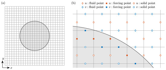
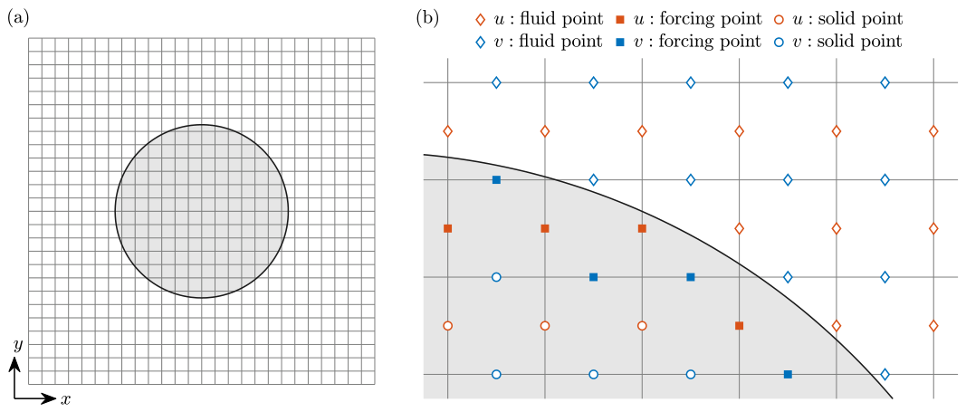
The issue of computing $u_{F,i}$ and ${\theta }_F$ when the interface does not coincide with grid nodes needs to be addressed. Figure 1 illustrates the definition of momentum forcing points on the Cartesian grid, where the cylindrical geometry is completely immersed in the fluid region. It is observed that the forcing points are the first internal grid nodes located within the solid body. The arrangement of energy forcing points is quite similar; the only difference is that they are defined on the cell centers. In Equations(9) and (10), the forces are determined such that the velocity/temperature at the forcing points agrees with a velocity/temperature that is interpolated using points from the physical flow region and on the immersed boundary. In the present work, the values of $u_{F,i}$ and ${\theta }_F$ are determined via second-order linear and bilinear interpolations [41,56] based on the approximations of ${\tilde{u}}_i$ and $\tilde{\theta }$.

Figure 1. (a) A cylindrical geometry overlaid on a regular 2D Cartesian grid. (b) Schematic diagram for the locations of the forcing, fluid, and solid points on the 2D Cartesian grid. The black solid line represents the immersed rigid boundary.

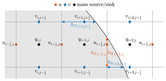
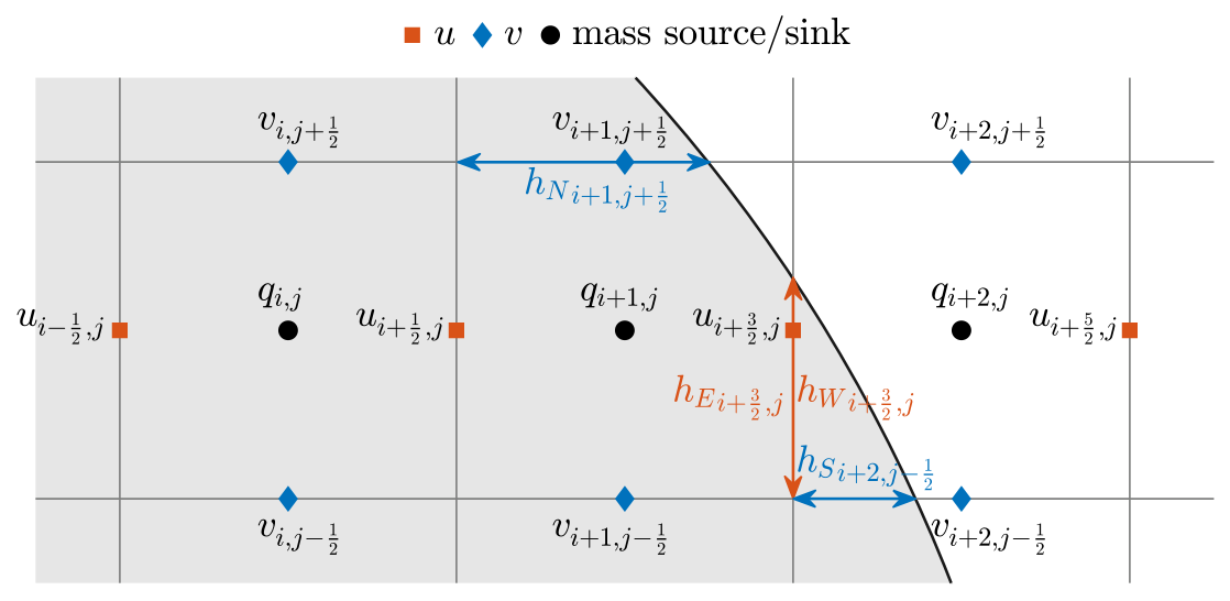
Most IBMs ensure mass conservation for every individual computational cell only, without taking the embedded boundary into account. When the interface cells are cut by the immersed boundary, mass conservation of the fluid portion is not valid, and mass exchange between the fluid and solid parts occurs. As a result, the non-physical solution inside the solid region can influence the accuracy of the physical solution in the fluid region [57]. For the convective flows considered here, this also affects the local accuracy of the temperature near the immersed boundary, as the temperature field is convected by the velocity. In the current work, we compute the mass source/sink on the cell faces that are cut by the fluid–solid interface, i.e., the computational cell faces containing both fluid and solid fractions. We also calculate the mass source/sink term for cells completely located in the solid region to preserve global mass conservation, since adjacent grid nodes sharing a common cell face have the same value of mass flux but opposite signs. A similar procedure has been adopted for simulation of moving body problems in Cartesian collocated grids [58] and in curvilinear coordinates [59], to reduce spurious force oscillations on the surface of the rigid body. As shown in Figure 2, in a 2D configuration with uniform grid spacings ($\Delta x$ and $\Delta y$ in the x and y coordinate directions), the mass source/sink term for interface cells or solid cells can be expressed in a discrete form as

$$q_{i,j}^{n+1}={\displaystyle \frac{1}{\Delta x\Delta y}}(-u_{i-{\displaystyle \frac{1}{2}},j}^{\prime }\Delta y-v_{i,j-{\displaystyle \frac{1}{2}}}^{\prime }\Delta x+u_{i+{\displaystyle \frac{1}{2}},j}^{\prime }\Delta y+v_{i,j+{\displaystyle \frac{1}{2}}}^{\prime }\Delta x),$$

(11)

$$q_{i+1,j}^{n+1}={\displaystyle \frac{1}{\Delta x\Delta y}}(-u_{i+{\displaystyle \frac{1}{2}},j}^{\prime }\Delta y-v_{i+1,j-{\displaystyle \frac{1}{2}}}^{\prime }\Delta x+u_{i+{\displaystyle \frac{3}{2}},j}^{\prime }{h_E}_{i+{\displaystyle \frac{3}{2}},j}\Delta y+v_{i+1,j+{\displaystyle \frac{1}{2}}}^{\prime }{h_N}_{i+1,j+{\displaystyle \frac{1}{2}}}\Delta x),$$

(12)

$$q_{i+2,j}^{n+1}={\displaystyle \frac{1}{\Delta x\Delta y}}(-u_{i+{\displaystyle \frac{3}{2}},j}^{\prime }{h_W}_{i+{\displaystyle \frac{3}{2}},j}\Delta y-v_{i+2,j-{\displaystyle \frac{1}{2}}}^{\prime }{h_S}_{i+2,j-{\displaystyle \frac{1}{2}}}\Delta x),$$

(13)

where indices such as i and j denote grid points of the numerical mesh and $h_W$, $h_E$, $h_S$, and $h_N$ are solid fractions of west, east, south, and north cell faces, respectively. These factors vary between 0 and 1 for boundary-cut cells, and they are equal to 1 for cells completely located in the solid region. For a circular immersed boundary, the interface cells are identified by comparing the distance from each cell vertex to the circle center against the known radius. If they are all located inside or outside the immersed boundary, then they are solid or fluid cells, respectively. Otherwise, they are interface cells. Subsequently, the solid fractions can be evaluated by computing the intersection points of the circle’s circumference with the cell edges based on the location of grid lines and cell vertices, as well as the function of the immersed boundary. Since no-slip and no-penetration velocity boundary conditions are implemented on the immersed boundary, there is no mass flux through the segment of the immersed boundary within the cell.

Figure 2. Schematic diagram for the calculation of the mass source/sink. The arrows represent the solid fractions of each cell face.

As mass source/sink (q) is calculated at both the interface and solid cell faces. This treatment differs from the original mass source/sink approach [38], which only considers that the cell vertices fall on the immersed boundary and just estimates the mass fluxes at the forcing points. Furthermore, compared with the improved IBM with a mass source/sink [39,58], interpolation of the face velocity at the center of a solid fraction is avoided for every time step. Once the solid fractions for each cell face are determined and stored during preprocessing, only an additional loop is needed at each time step to modify the right-hand side of the pressure Poisson equation. This procedure is also similar to the Cartesian cut-cell methods to some extent, as it discards the solid part of the interface cell but does not construct new polyhedral cells [28]. Furthermore, because the velocity components at time step $n+1$ are currently unknown for calculation of the mass source/sink term, they are approximated using the intermediate velocities ($u^{\prime }$ and $v^{\prime }$) in the above expressions by neglecting the pressure-gradient term, given that the face center of interface cells crossed by the solid boundary is the first node outside or inside the rigid boundary. For the former case, the homogeneous Neumann condition is implemented for pressure on the boundary; for the latter case, the pressure in the solid region is unphysical. This implementation enables us to solve the pressure field in both fluid and solid regions. The algorithm is first-order accurate in time, in line with the original standard projection method [54], as $u_i^{n+1}=u_i^{\prime }-(2\Delta t/3)(\partial p^{n+1}/\partial x_i)=u_i^{\prime }+O(\Delta t)$.

3. Verification and Validation

3.1. Accuracy Test with Convective Flow Induced by a Rotating Solid Disk

To verify the spatial accuracy of the presented numerical algorithm, we simulate forced convection (the influence of the buoyancy term in the momentum equation is neglected) induced by a solid disk rotating clockwise at constant tangential velocity ($u_t$) within a 2D square enclosure ($0⩽x,y⩽1$). The disk, with a radius of $r=0.15$, is positioned at the center of the computational domain. The considered flow is laminar with a Reynolds number of $Re=100$ based on the cavity length (L) and the disk’s peripheral velocity ($u_t$). The Prandtl number is chosen as $Pr=0.71$. We impose no-slip boundary conditions on all solid walls and conduct five computations on progressively finer uniform grids: $24\times 24$, $48\times 48$, $96\times 96$, $192\times 192$, and $384\times 384$. For the temperature boundary conditions, both the isothermal (Dirichlet-type) and adiabatic (Neumann-type) surfaces of the solid disk are considered. In the former case, the temperatures on the inner hot and outer cold surfaces are set as ${\theta }_{\mathrm{in}}=1$ and ${\theta }_{\mathrm{out}}=0$, respectively; in the latter case, the bottom and top walls of the cavity are heated and cooled at constant temperatures of ${\theta }_{\mathrm{bot}}=1$ and ${\theta }_{\mathrm{top}}=0$, respectively, while the left and right boundaries of the cavity and the disk surface are adiabatic.

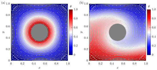
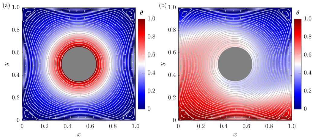
Figure 3a,b present the temperature contours and streamlines for isothermal and adiabatic boundary conditions, respectively, in the steady state for the finest grid. A converged solution is obtained by iterating in time until variations in the primitive variables between subsequent time steps is very small, i.e., $\sqrt{\Sigma {({\zeta }_{i,j}^{n+1}-{\zeta }_{i,j}^n)}^2}/\sqrt{\Sigma {\left({\zeta }_{i,j}^{n+1}\right)}^2}<{10}^{-8}$, where $\zeta$ stands for horizontal velocity (u), vertical velocity (v), or temperature ($\theta$). The rotation of the fluid around the cylinder can be clearly observed, and four tiny vortex rolls are observed at the corners.

Figure 3. Temperature contours and streamlines of convective flow induced by a rotating solid disk with (a) isothermal and (b) adiabatic surfaces. The grey lines stand for the streamlines, the arrows stand for the direction of velocity, and the colorbars stand for the value of temperature.

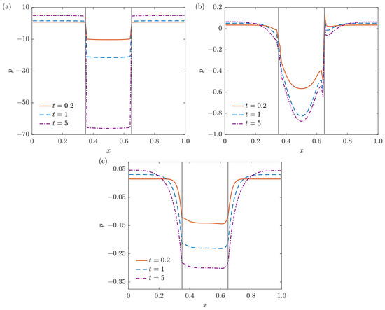
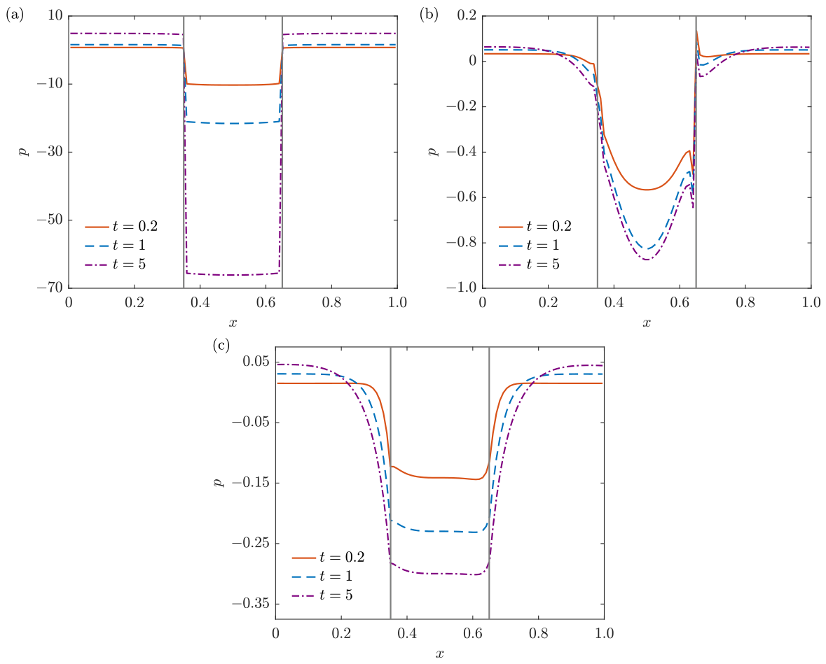
When a discrete-forcing immersed boundary method is applied to moving-body problems, it produces spurious force oscillations on a solid body. One source is from the spatial discontinuity in the pressure across the immersed boundary, as revealed by Lee et al. [60]. To compare the current method with the approach without a source/sink term in the continuity equation and the original one proposed by Kim et al. [38], Figure 4a–c show the pressure distributions along the horizontal centerline ($y=0.5$) of the cylinder at different instants without and with the mass source/sink (q) obtained from the moderate spatial resolution with $96\times 96$ grid cells. It is clearly seen from Figure 4a that a pressure jump across the body surface exists, and the magnitude of p inside the cylinder increases significantly with increasing time. This is caused by the non-fulfillment of continuity due to the projection step in the solution procedure, which alters the interpolated velocity at the forcing point [36,58]. With the method proposed by Kim et al. [38], the strong pressure jump near the immersed boundary is suppressed, as shown in Figure 4b. However, pressure oscillations can be identified at the fluid–solid interface (for instance, at $x\approx 0.65$), as the mass source/sink (q) is only estimated at the forcing points close to the immersed boundary. Thus, the original approach is suitable for stationary-body problems, but not for the current flow induced by a rotating boundary. As shown in Figure 4c, by using the modified mass source/sink (q), the continuity is satisfied by the formulation, and the pressure inside the solid region is not very different from that in the fluid region near the immersed boundary, i.e., no pressure jumps or obvious oscillations are observed. Thus, it is confirmed that the presented modification of the mass source/sink has an effective influence on the numerical solution.

Figure 4. The pressure profile along $y=0.5$ at different instants obtained by (a) the traditional IBM without a mass source/sink, (b) the original approach introduced by Kim et al. [38], and (c) the modified source/sink method. The two vertical gray lines denote the location of the immersed boundary.

As the intermediate velocities ($u^{\prime }$ and $v^{\prime }$) are used to calculate the mass source/sink (q), an error could be introduced in the continuity equation. To better understand this issue, we examine the local mass imbalance estimated by

$$E_{i,j}=\left[\left({\displaystyle \frac{u_{i+\frac{1}{2},j}-u_{i-\frac{1}{2},j}}{\Delta x}}+{\displaystyle \frac{v_{i,j+\frac{1}{2}}-v_{i,j-\frac{1}{2}}}{\Delta y}}\right)-q_{i,j}\right]\Delta x\Delta y.$$

(14)

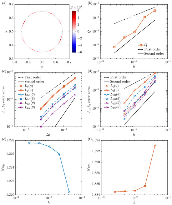
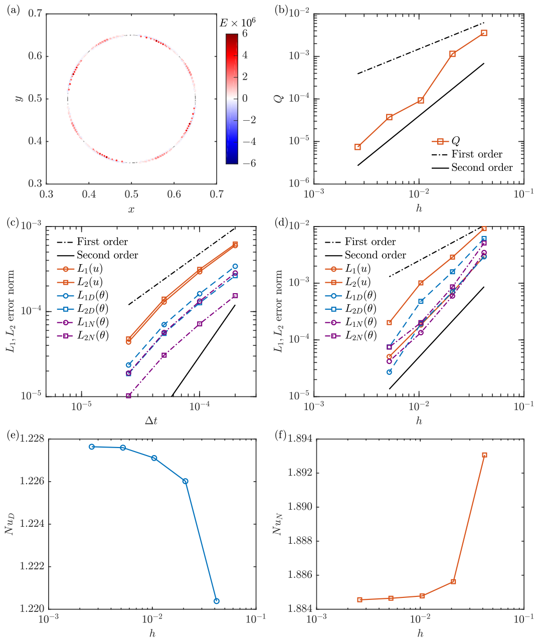
Figure 5a displays the distribution of $E_{i,j}$ in the vicinity of the immersed boundary for the finest grid. It is found that larger values of $E_{i,j}$ are concentrated in the interface cells cut by the immersed boundary, with magnitude well restrained, while the maximum absolute value of $E_{i,j}$ is about $6\times {10}^{-6}$. Additionally, the summation of $E_{i,j}$ in the solid and interface cells indicates that the integral mass imbalance reaches machine precision (around ${10}^{-16}$). As the mass source/sink (q) serves as a correction term in the continuity equation, we also present the averaged mass source/sink ($Q=-{\Sigma }_1^{n_i}{q}_{i,j}\Delta x\Delta y/n_i$) in Figure 5b to better understand how it is influenced by spatial resolution. Here, $n_i$ is the number of interface cells cut by the immersed boundary. We can see that the averaged mass source/sink decays at an approximately second-order rate as the spatial resolution increases.

Figure 5. (a) Local mass imbalance ($E_{i,j}$) in the vicinity of the immersed boundary. (b) Averaged mass source/sink (Q) as a function of grid spacing. $L_1$ and $L_2$ error norms for horizontal velocity (u), as well as temperature ($\theta$), as a function of (c) the time-step size and (d) the grid spacing. Subscripts D and N stand for the Dirichlet and Neumann boundary conditions for the temperature on the surface of the solid disk. The surface-averaged Nusselt numbers along the bottom plate as a function of grid spacing for both the Dirichlet (e) and Neumann (f) boundary conditions.

To inspect errors in the velocity and temperature fields, we use the simulation results at the finest grid or time step as the reference. The $L_1$ and $L_2$ norms of the error, which are the differences between the solutions at the coarsest and finest resolutions, are defined as

$$L_1\left({\zeta }_i\right)={\displaystyle \frac{1}{n_g}}{\displaystyle \sum _{n=1}^{n_g}}|{\zeta }_i^c\left(n\right)-{\zeta }_i^r\left(n\right)|,$$

(15)

$$L_2\left({\zeta }_i\right)=\sqrt{{\displaystyle \frac{1}{n_g}}\sum _{n=1}^{n_g}{[{\zeta }_i^c\left(n\right)-{\zeta }_i^r\left(n\right)]}^2}.$$

(16)

In the formulations above, $n_g$ is the total number of grid points in the fluid region (considering that the flow within the solid region is unphysical), and ${\zeta }_i^c$ and ${\zeta }_i^r$ are the numerical solutions of u and $\theta$ from the coarse and reference solutions, respectively. The grid spacings in both the x and y directions are fixed at $\Delta x=\Delta y=1/128$ for a temporal convergence study. Numerical simulations are performed until $t=0.1$ using five distinct time-step sizes. The resulting $L_1$ and $L_2$ error norms, as a function of the time step size ($\Delta t$), are presented in Figure 5c. As expected, the implementation of the standard projection method yields first-order temporal accuracy. The $L_1$ and $L_2$ error norms, as a function of the spatial resolution ($h=1/n_x=1/n_y$), are shown in Figure 5d. It is observed that the errors decrease with an approximately second-order slope, indicating that the presented method is second-order accurate in space. To ensure spatial discretization errors are minimized, the Grid Convergence Index (GCI) [61] was calculated for the surface-averaged Nusselt numbers ($Nu={\int }_0^1{\displaystyle \frac{\partial \theta }{\partial y}}{|}_{y=0}\mathrm{d}x$) along the bottom plate. The dependence of $Nu$ on the grid spacing (h) is illustrated in Figure 5e,f. For both the Dirichlet and Neumann boundary conditions, the GCI values for the finest grid resolutions are below $0.1\%$, confirming that the solutions lie well within the asymptotic convergence range. It should be noted that the time step in the reported simulations is limited, as the explicit forcing method is utilized. Numerical tests show that it is limited by the viscous stability because of the errors in the diffusion terms rather than the Courant–Friedrichs–Lewy constraint, and the method remains stable for $\Delta t<\min [Re{h}^2/6,RePr{h}^2/6]$.

3.2. Forced Convection over an Isothermal Rotating Circular Cylinder

The uniform flow across a circular cylinder has been intensively investigated, and it is commonly used to verify the accuracy of IBMs. The flow structures depend on the Reynolds number ($Re=u_{\infty }d/\nu$), which is based on the far-field velocity ($u_{\infty }$) and the cylinder diameter (d). For $Re$ values below 47, the wake behind a (non-rotating) cylinder remains symmetric, with a steady recirculation zone established behind the cylinder [62]. At higher Reynolds numbers, the flow undergoes a symmetry-breaking instability, resulting in the well-known phenomenon of periodic vortex shedding, commonly referred to as the Karman vortex street. However, the rotation of a cylinder within a viscous, uniform flow alters the wake dynamics and vortex-shedding properties, and the flow behavior depends not only on the Reynolds number ($Re$) but also on the dimensionless parameter ($k=u_t/u_{\infty }$), which represents the ratio of the peripheral velocity ($u_t$) to the inflow velocity ($u_{\infty }$). In this subsection, forced convection flows at Reynolds numbers of $Re=40$ and 100 are simulated at $k=0$ (the cylinder is stationary) and 1 (the cylinder is rotating clockwise, with the peripheral velocity ($u_t$) equal to $u_{\infty }$). The Prandtl number is chosen as $Pr=0.71$, whereas the Grashof number is specified as $Gr=0$.

We consider flow in a 2D rectangular domain with $0⩽x⩽36d$ and $0⩽y⩽18d$, where the fluid flows from the left to the right. The cylinder is positioned at $(x,y)=(12d,9d)$, and the diameter (d) is set as 1. A uniform flow of $(u_{\infty },v)=(1,0)$ is prescribed at the inlet ($x=0$), the top and bottom velocity boundary conditions are imposed as $\partial u/\partial y=0$ and $v=0$, and a zero-gradient velocity boundary condition of $\partial u/\partial x=\partial v/\partial x=0$ is applied at the outlet. The temperature values at the cylinder surface and at the far stream are 1 and 0, respectively. On the top, bottom, and right boundaries, the heat flux is specified as 0. As for the pressure boundary condition, the outlet pressure is fixed as $p=0$, and the Neumann condition is applied to all other boundaries. We test two different meshes to cover the whole domain; their grid numbers are $1024\times 512$ and $1536\times 768$ in the streamwise (x) and transverse (y) directions, respectively. The grids are uniformly distributed with grid spacings of $0.03515625d$ and $0.0234375d$.

For comparison, we calculate the forces on the cylinder surface after the flow has converged to a steady or periodic state. The drag force ($f_D$) and lift force ($f_L$) acting on the cylinder due to pressure and viscous forces are expressed as [63]

$$f_D={\int }_0^{2\pi }{\displaystyle \frac{d}{2}}[-pcos\left(\alpha \right)-\nu \omega sin\left(\alpha \right)]\mathrm{d}\alpha ,$$

(17)

$$f_L={\int }_0^{2\pi }{\displaystyle \frac{d}{2}}[-psin\left(\alpha \right)+\nu \omega cos\left(\alpha \right)]\mathrm{d}\alpha ,$$

(18)

where $\alpha$ is the angular position on the cylinder surface, measured from the downstream stagnation point. The drag coefficient ($C_D$) and lift coefficient ($C_L$) are calculated as

$$C_D={\displaystyle \frac{f_D}{\frac{1}{2}\rho u_{\infty }^{2}d}},$$

(19)

$$C_L={\displaystyle \frac{f_L}{\frac{1}{2}\rho u_{\infty }^{2}d}},$$

(20)

where $\rho =1$ is the fluid density. The Strouhal number ($St$) characterizing the periodic shedding of the vortices is formulated as

$$St={\displaystyle \frac{fd}{u_{\infty }}}.$$

(21)

Here, f is the vortex-shedding frequency calculated by the fast Fourier transform of the time evolution of the lift coefficient ($C_L$). In the current work, the fast Fourier transform was performed using a sampling duration of $t=150$ after the flow reached a periodic state. The Strouhal number was then estimated from the dominant frequency peak in the power spectral density. Another dimensionless quantity of interest is the Nusselt number, which describes the heat-transfer efficiency. The local and surf-averaged values of flow past an isothermal circular cylinder are computed as

$$N{u}_{\mathrm{local}}=-{\displaystyle \frac{\partial \theta }{\partial n}}{|}_{\mathrm{wall}},$$

(22)

$$N{u}_{\mathrm{mean}}=-{\displaystyle \frac{1}{S}}{\int }_0^S{\displaystyle \frac{\partial \theta }{\partial n}}{|}_{\mathrm{wall}}\mathrm{d}S,$$

(23)

where n denotes the normal direction of the cylinder surface and S corresponds to the circumferential length of the isothermal cylinder.

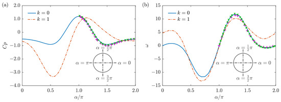
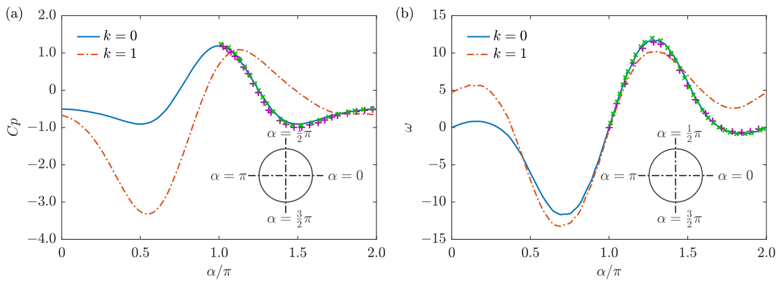
The pressure coefficient ($C_p$) and vorticity ($\omega$) along the cylinder surface, as a function of the angular position ($\alpha$) for the steady case at $Re=40$, are given in Figure 6a,b, respectively. Here, the wall-pressure coefficient ($C_p$) is defined as

$$C_p={\displaystyle \frac{p-p_{\infty }}{\frac{1}{2}\rho u_{\infty }^2}},$$

(24)

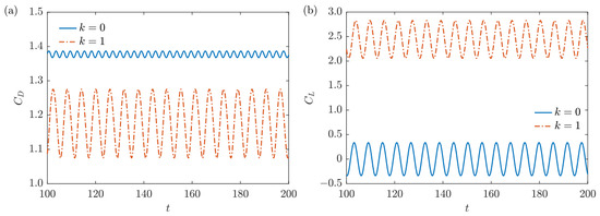
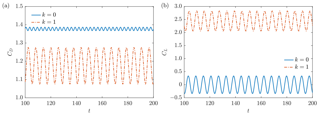
where $p_{\infty }=0$ is the ambient pressure. In the figure, numerical results obtained with the IBMs of Tseng and Ferziger [25] and of Berthelsen and Faltinsen [64] at $k=0$ are plotted for comparison as well. The figures reveal that the pressure coefficient ($C_p$) at $k=0$ is symmetric about $\alpha =\pi$, and the vorticity ($\omega$) is antisymmetric about $\alpha =\pi$. As k increases, the flow becomes asymmetric, and the pressure on the upper side of the cylinder decreases due to the acceleration of the flow. On the other hand, the vorticity ($\omega$) is nearly zero in the wake for $k=0$; however, its magnitude increases significantly in the wake region at $k=1$. For the unsteady case, Figure 7a,b illustrate the time evolution of drag and lift coefficients at $Re=100$, showing that rotating the cylinder causes a smaller drag coefficient, and the mean value of the lift coefficient is no longer zero. Due to the Magnus effect, the flow is accelerated on the upper side of the cylinder and decelerated on the lower side of it. Consequently, the pressure on the accelerated side is lower than that on the decelerated side, resulting in a mean lift force. It should also be noted that the oscillating frequency of $C_D$ is twice that of $C_L$ for the stationary case ($k=0$), which is the vortex-shedding frequency (f).

Figure 6. (a) Pressure coefficient ($C_p$) and (b) vorticity ($\omega$) on the cylinder surface as a function of the angular position ($\alpha$) at a Reynolds number of $Re=40$. The numerical results obtained with the IBMs of Tseng and Ferziger [25] and Berthelsen and Faltinsen [64] at $k=0$ are labeled as ‘+’ and ‘×’, respectively.

Figure 7. (a) Drag coefficient ($C_D$) and (b) lift coefficient ($C_L$) as a function of time t at a Reynolds number of $Re=100$.

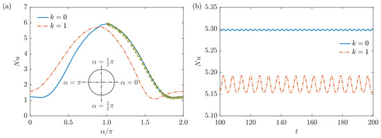
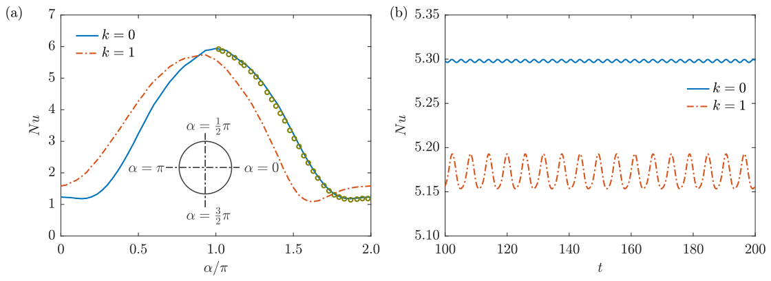
Figure 8a shows how the local Nusselt number varies on the cylinder surface at $Re=40$. When the cylinder is stationary, $Nu$ peaks near the front stagnation point at $\alpha =\pi$ and gradually decreases along the cylinder surface, and the distribution of $Nu$ is in line with the result reported by Das et al. [65]. As the cylinder rotates, the shear effect increases on the upper side, thinning the thermal boundary layer and making $Nu$ greater in that area. At $Re=100$, the flow becomes unsteady, and the temperature field becomes asymmetric and varies periodically with time, as confirmed by the time histories of the surface-averaged $Nu$ given in Figure 8b. This figure also shows that the magnitude of the Nusselt number decreases as the rotation rate increases. The reason is that the enveloping vortex grows larger, and the fluid entrapped inside it acts as a buffer zone for heat transfer between the cylinder and the free stream [2].

Figure 8. (a) Local Nusselt number on the cylinder surface as a function of the angular position ($\alpha$) at a Reynolds number of $Re=40$. The distribution of $Nu$ obtained with the IBM of Das et al. [65] at $k=0$ is labeled as ‘∘’ for comparison. (b) Time histories of the surface-averaged Nusselt number at $Re=100$.

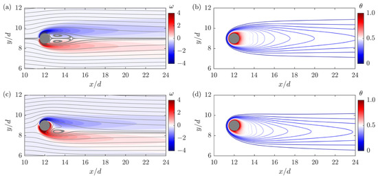
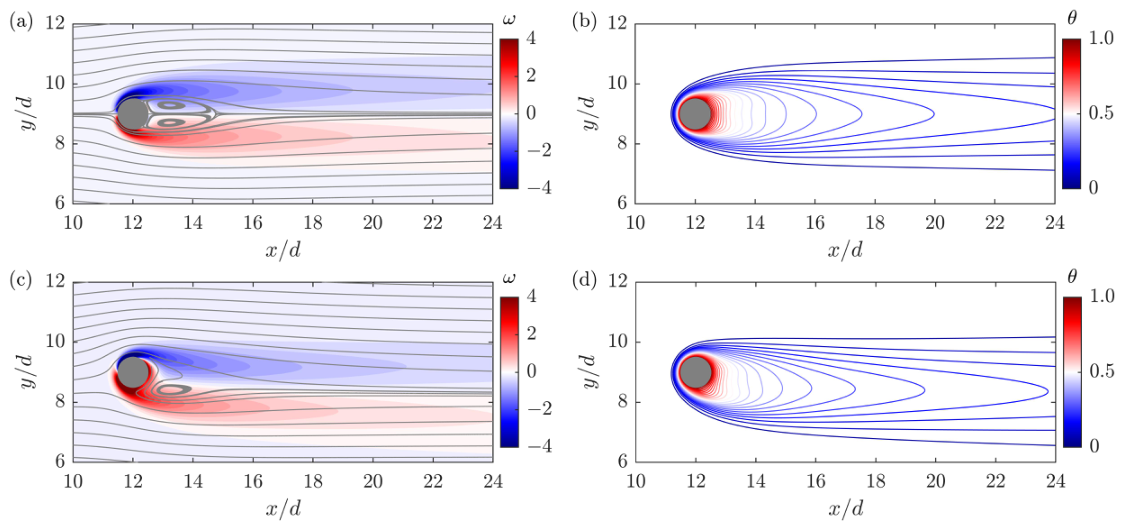
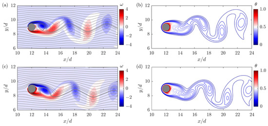
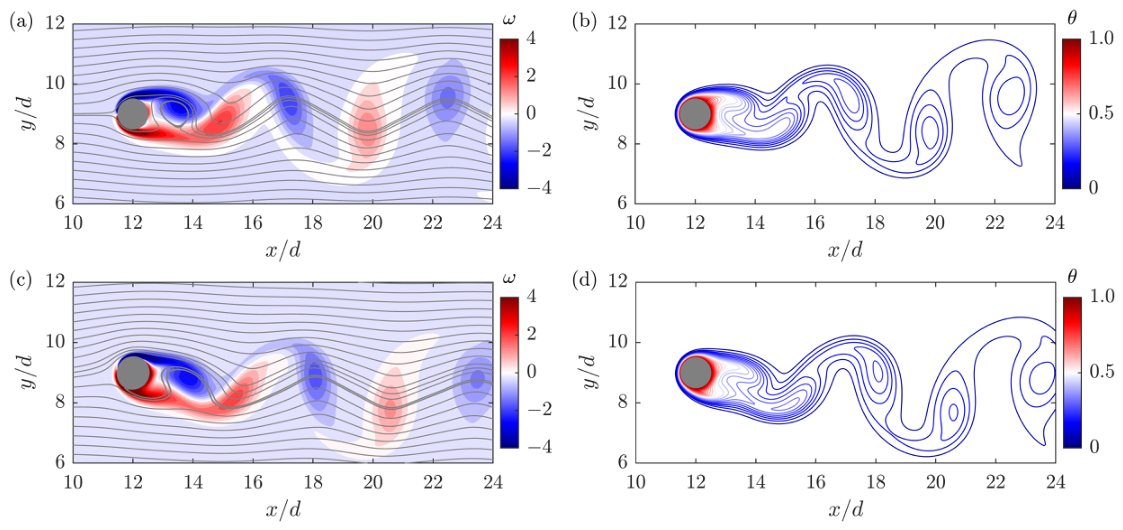
The vorticity contours, streamlines, and isotherms for the simulation cases at $Re=40$ and 100 are presented in Figure 9 and Figure 10, respectively. It is observed that no vortex shedding develops, regardless of the value of k in the case of $Re=40$. The flow is symmetric, with a pair of stationary recirculating vortices attached behind the cylinder for $k=0$. Being different, rotating delays the flow separation, the upper vortex disappears, and the lower one detaches from the cylinder surface at $k=1$. In contrast, the symmetry of the flow breaks down, and two vortices are shed alternatively at $Re=100$. In the near-surface flow, as k increases, the negative vorticity on the upper side of the cylinder becomes more dominant than the positive vorticity on the lower side.

Figure 9. (a) Vorticity contours superimposed with streamlines and (b) isotherms for forced convection over a circular cylinder at a Reynolds number of $Re=40$ with a velocity ratios of $k=0$. (c) Vorticity contours superimposed with streamlines and (d) isotherms for forced convection over a circular cylinder at a Reynolds number of $Re=40$ with a velocity ratios of $k=1$. The vorticity contour interval is specified as 0.08, and the temperature contour interval is 0.04.

Figure 10. (a) Vorticity contours superimposed with streamlines and (b) isotherms for forced convection over a circular cylinder at a Reynolds number of $Re=100$ with a velocity ratios of $k=0$. (c) Vorticity contours superimposed with streamlines and (d) isotherms for forced convection over a circular cylinder at a Reynolds number of $Re=100$ with a velocity ratios of $k=1$. The vorticity contour interval is specified as 0.08, and the temperature contour interval is 0.04.

To quantitatively compare the current results with previous numerical predictions, Table 1 and Table 2 summarize the length of the recirculation zone ($L_w$), the drag coefficient ($C_D$), the lift coefficient ($C_L$), the amplitude of the drag fluctuation ($C_D^{\prime }$), the amplitude of the lift fluctuation ($C_L^{\prime }$), the Strouhal number ($St$), and the Nusselt number ($Nu$), alongside those from the references. For $Re=40$, the flow is laminar; hence, the drag and lift coefficients, as well as the Nusselt number, remain constant. In addition, as the flow is symmetric at $k=0$, the lift coefficient ($C_L$) is 0. It also demonstrates the results obtained from the coarse and fine meshes are very close, and the error is less than $1\%$ for most of the quantities. For this reason, the finer grid is used to simulate flow at $Re=100$. In Table 2, $C_D$, $C_L$, and $Nu$ are reported as their mean or time-averaged values for $Re=100$. Although rotation of a cylinder changes the lift and drag coefficients and Nusselt number, it does not obviously alter $St$ in the parameter range considered here. In general, the presented numerical results agree well with those of previous investigations, demonstrating the capability of the present method for simulating flow involving a spinning cylinder.

Table 1. Comparison of wake length ($L_w$), drag coefficient ($C_D$), lift coefficient ($C_L$), and Nusselt number ($Nu$) with those obtained in previous numerical studies for $Re=40$.

Reference	$\mathit{k}=0$			$\mathit{k}=1$
	${\mathit{L}}_{\mathit{w}}$	${\mathit{C}}_{\mathit{D}}$	$\mathit{Nu}$	${\mathit{C}}_{\mathit{D}}$	${\mathit{C}}_{\mathit{L}}$	$\mathit{Nu}$
Badr and Dennis [66]						3.405
Sufyan et al. [6]			3.310			3.260
Soares and Rouboa [67]			3.240			3.199
Jagad et al. [63]	2.28	1.605
Panda and Chhabra [68]		1.5136			1.3233	2.599
Luo et al. [69]	2.17	1.578	3.2466
Xu and Choi [49]		1.643	3.278
Present study (coarse grid)	2.25	1.5557	3.355	1.4023	2.4517	3.305
Present study (fine grid)	2.25	1.5783	3.335	1.4046	2.5559	3.288

Table 2. Comparison of drag coefficient ($C_D$), lift coefficient ($C_L$), amplitude of the drag fluctuation ($C_D^{\prime }$), amplitude of the lift fluctuation ($C_L^{\prime }$), Strouhal number ($St$), and Nusselt number ($Nu$) with those obtained in previous numerical studies for $Re=100$.

	Reference	${\mathit{C}}_{\mathit{D}}$	${\mathit{C}}_{\mathit{L}}$	${\mathit{C}}_{\mathit{D}}^{\prime }$	${\mathit{C}}_{\mathit{L}}^{\prime }$	$\mathit{St}$	$\mathit{Nu}$
$k=0$	Mahfouz and Badr [70]					0.16	5.31
	Mahir and Altaç [71]	1.368			0.343	0.172	5.179
	Stojković et al. [72]	1.3371		0.0091	0.3259	0.1650
	Dalal et al. [73]	1.4147				0.1587	5.3523
	Luo et al. [69]	1.337				0.169
	Xu and Choi [49]	1.382			0.359		5.100
	Present study (fine grid)	1.3772		0.0097	0.3385	0.1697	5.298
$k=1$	Badr and Dennis [66]						5.139
	Paramane and Sharma [2]	1.0951	2.49	0.0981	0.3461	0.1645
	Kang et al. [62]	1.0979	2.4833	0.0988	0.3603	0.1650
	Stojković et al. [72]	1.1080	2.504	0.0986	0.3616	0.1658
	Present study (fine grid)	1.1801	2.4444	0.1006	0.3866	0.1697	5.170

3.3. Mixed Rayleigh–Bénard Convection with an Adiabatic Rotating Circular Cylinder

In this subsection, we consider mixed Rayleigh–Bénard convection within a square cavity containing a uniformly rotating circular cylinder. In this scenario, the velocity and temperature fields are coupled, and the Oberbeck–Boussinesq approximation is used. Previous investigations of mixed convection in a square cavity mainly focused on flow confined between laterally heated vertical plates [8,74]; however, it is not clear how the internal rotating cylinder affects the heat-transport properties of Rayleigh–Bénard convection. Here, we put the circular cylinder at the cavity center to avoid any geometrical asymmetry of the flow configuration. The length (L) of the cavity is 1, and the radius (r) of the circular cylinder is changed during the simulation. The bottom and top walls of the cavity are heated and cooled at constant temperatures of ${\theta }_{\mathrm{bot}}=1$ and ${\theta }_{\mathrm{top}}=0$, respectively, while the left and right boundaries of the cavity are adiabatic. A no-slip velocity boundary condition is imposed on all the solid walls of the cavity. The cylinder surface is adiabatic ($\partial \theta /\partial r=0$), rotating at a constant clockwise tangential velocity of $u_t$.

Apart from the Rayleigh number ($Ra$) and the Prandtl number ($Pr$), which influence convective motion, the flow is also controlled by the Reynolds number ($Re=u_{t}L/\nu$), representing the dimensionless rotating speed. The current work fixes the Rayleigh number at $Ra={10}^5$ and investigates the influences of the Prandtl number ($Pr=0.1$, 1, 10), rotating speed ($0⩽Re⩽1000$), and cylinder radius ($r=0.1$, 0.2, 0.3, 0.4). The system’s response parameter is the Nusselt number ($Nu$), which is calculated based on the heat flux at the bottom and top conducting plates of the container as follows:

$$Nu=-{\displaystyle \frac{1}{2}}\left({\int }_0^1{\displaystyle \frac{\partial \theta }{\partial y}}{{|}_{y=0}\mathrm{d}x+{\int }_0^1{\displaystyle \frac{\partial \theta }{\partial y}}|}_{y=1}\mathrm{d}x\right).$$

(25)

Grid-function convergence tests are conducted using two uniform grids of $192\times 192$ and $384\times 384$ cells for all three Prandtl numbers at a Reynolds number of $Re=1000$ and cylinder radius of $r=0.4$. Table 3 presents a comparison of the calculated Nusselt number ($Nu$) for the two different uniform grids, which shows that the differences between the coarser and finer grids are less than $0.125\%$ for the three cases. Therefore, the $192\times 192$ uniform grid is fine enough for the considered flow, and it is adopted in the following simulated cases.

Table 3. Comparison of Nusselt numbers ($Nu$) for the coarse and fine grids at $r=0.4$ and $Re=1000$.

Grid	$\mathit{Pr}=0.1$	$\mathit{Pr}=1$	$\mathit{Pr}=10$
$192\times 192$	4.6526	6.7565	14.9736
$384\times 384$	4.6468	6.7564	14.9815

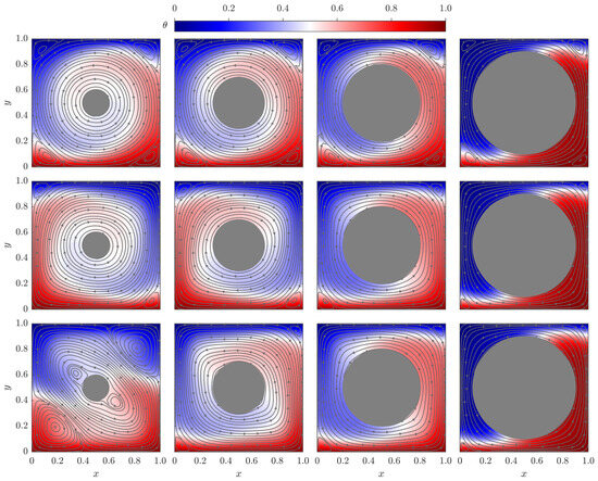
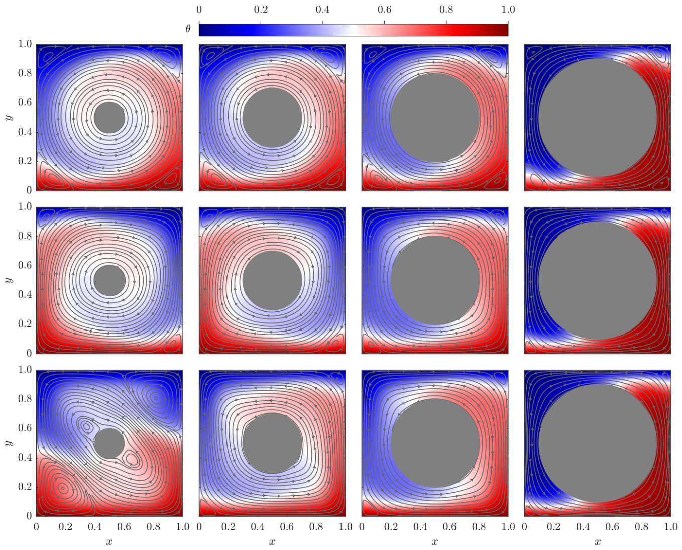
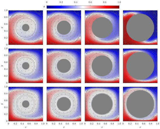
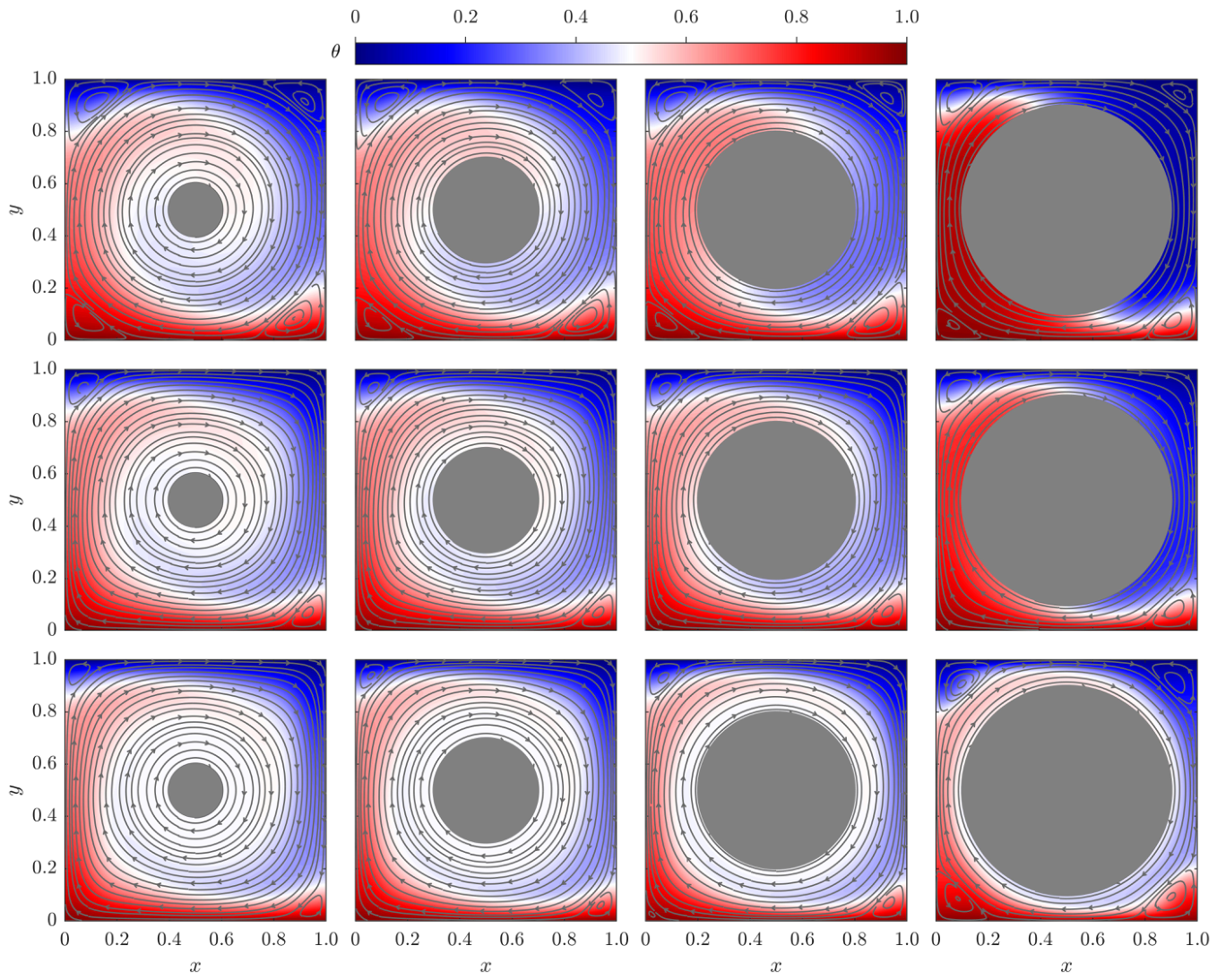
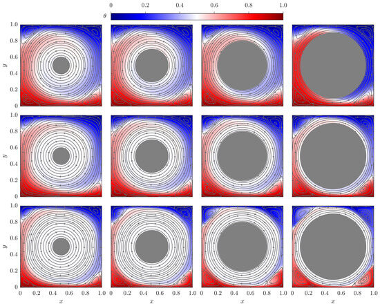
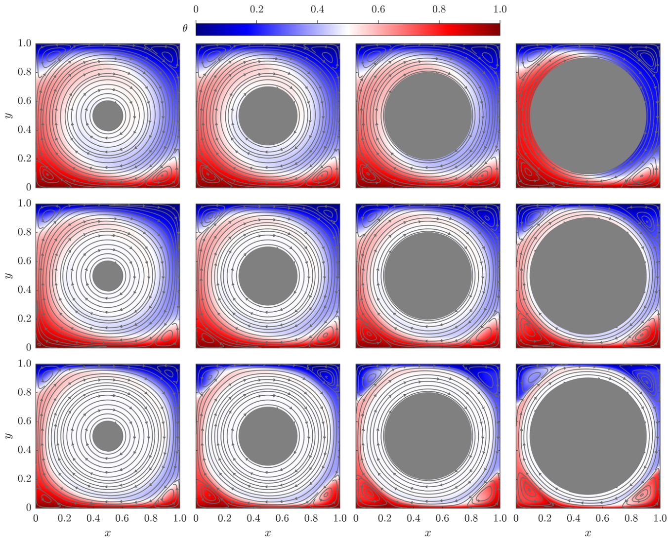
Effects of the spinning cylinder on flow patterns at three different $Re$ values are depicted in Figure 11, Figure 12 and Figure 13, where the temperature contours and streamlines are shown for various values of the Prandtl number and cylinder radius. All the numerical simulations are conducted until the flow converges to a steady state, except for the case at $r=0.1$, $Pr=10$, and $Re=0$, where a periodic flow state is found. When $Re=0$ (the cylinder is stationary), Figure 11 shows that the fluid moves along the periphery of the annulus, forming a large-scale clockwise or anticlockwise circulation roll occupying almost the entire flow domain, which is driven by the two system-sized plume columns. A noticeable difference is observed at $r=0.1$ and $Pr=10$, where obvious secondary rolls are generated close to the cylinder surface and in the corner region.

Figure 11. Temperature contours and streamlines for different values of Prandtl numbers (from top to bottom: $Pr=0.1$, 1, and 10) and cylinder radius (from left to right: $r=0.1$, 0.2, 0.3, and 0.4) at $Re=0$. The grey lines stand for the streamlines, the arrows stand for the direction of velocity, and the colorbars stand for the value of temperature.

Figure 12. Temperature contours and streamlines for different values of Prandtl numbers (from top to bottom: $Pr=0.1$, 1, and 10) and cylinder radius (from left to right: $r=0.1$, 0.2, 0.3, and 0.4) at $Re=100$. The grey lines stand for the streamlines, the arrows stand for the direction of velocity, and the colorbars stand for the value of temperature.

Figure 13. Temperature contours and streamlines for different values of Prandtl numbers (from top to bottom: $Pr=0.1$, 1, and 10) and cylinder radius (from left to right: $r=0.1$, 0.2, 0.3, and 0.4) at $Re=1000$. The grey lines stand for the streamlines, the arrows stand for the direction of velocity, and the colorbars stand for the value of temperature.

When a clockwise-rotating cylinder is introduced in the cavity center, Figure 12 and Figure 13 show that the large-scale circulating roll remains fixed in the clockwise direction. At $Pr=0.1$, regardless of the rotating direction, the temperature fields for these two Reynolds numbers ($Re=100$ and 1000) are very similar to the cases at $Re=0$. By contrast, the temperature contours change noticeably due to the circumferential shear force at larger $Pr$ values. Thermal plumes concentrate more in the side-wall regions, and the thermal boundary layer becomes thinner (note that the thickness of the thermal boundary layer thickness (${\delta }_{th}$) in Rayleigh–Bénard convection can be calculated as ${\delta }_{th}=1/\left(2Nu\right)$ [75,76], which is proportional to the inverse of the global heat-transport efficiency given below), especially at higher $Re$ values. Additionally, the corner rolls are larger in size because of the stronger shear force. Furthermore, for $r=0.1$ and $Pr=10$, any rotation rate of the embedded cylinder causes a steady flow within the explored parameter range, demonstrating that adding shear to the system could stabilize the flow.

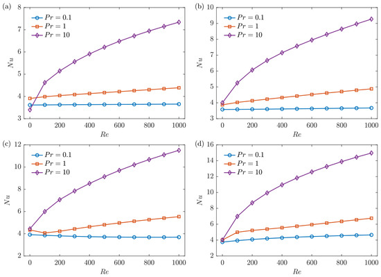
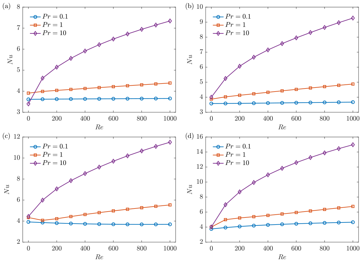
We now present the heat-transfer efficiency for the numerical simulation results. Figure 14 plots the relationship between the Nusselt number ($Nu$) and the dimensionless rotating speed ($Re$) obtained from various values of the Prandtl number ($Pr$) at each cylinder radius (r). It is generally found that, at a given $Re$, $Nu$ is greater with larger $Pr$ values, independent of the cylinder radius (r). Again, exceptions are observed at $r=0.1$, $Pr=10$, and $Re=0$. The reason is that the flow is unstable, and the competition between the main vortex and corner rolls can hinder the heat transfer [54,77]. Figure 14 also shows that, for most of the simulation cases, rotating the immersed cylinder enhances the heat-transfer rate, and a consistently decreasing $Nu$ with respect to $Re$ is only observed at $r=0.3$ for $Pr=0.1$. Additionally, the distributions of $Nu$ at different r values are quite similar: the $Re$ dependence of $Nu$ is very weak at $Pr=0.1$ (the largest difference is around $5.8\%$ at $r=0.3$ and $Re=1000$ when compared with the stationary cylinder case), whereas it increases considerably with an increasing $Re$ at a larger Prandtl number of $Pr=10$ (the enhancement is $272.2\%$ at $r=0.4$ and $Re=1000$). These observations are consistent with the temperature contours shown in Figure 11, Figure 12 and Figure 13, where the flow is shown to be buoyancy-dominated at smaller $Pr$ values, while it is shear-dominated at larger $Pr$ values. To measure the relative strength between the two driving buoyancy and shear forces, we can define the Richardson number ($Ri=Ra/\left(PrR{e}^2\right)$), which gives $Ri⩾1$ for $Pr=0.1$ and $Ri⩽1$ for $Pr=10$ in the Reynolds-number range of $100⩽Re⩽1000$, confirming the above statement.

Figure 14. The Nusselt number ($Nu$) as a function of the Reynolds number ($Re$) at different Prandtl numbers ($Pr$) for cylinder radii of (a) $r=0.1$, (b) $r=0.2$, (c) $r=0.3$, and (d) $r=0.4$.

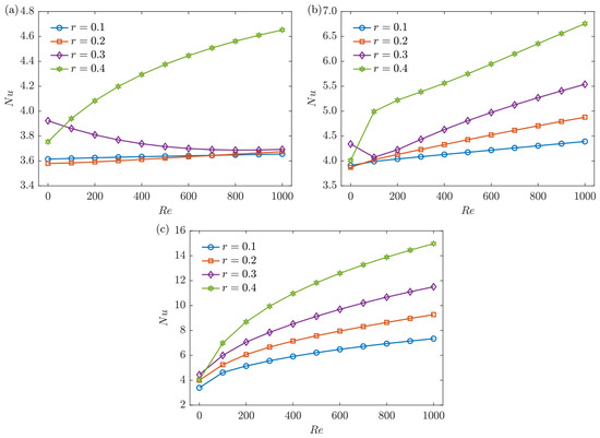
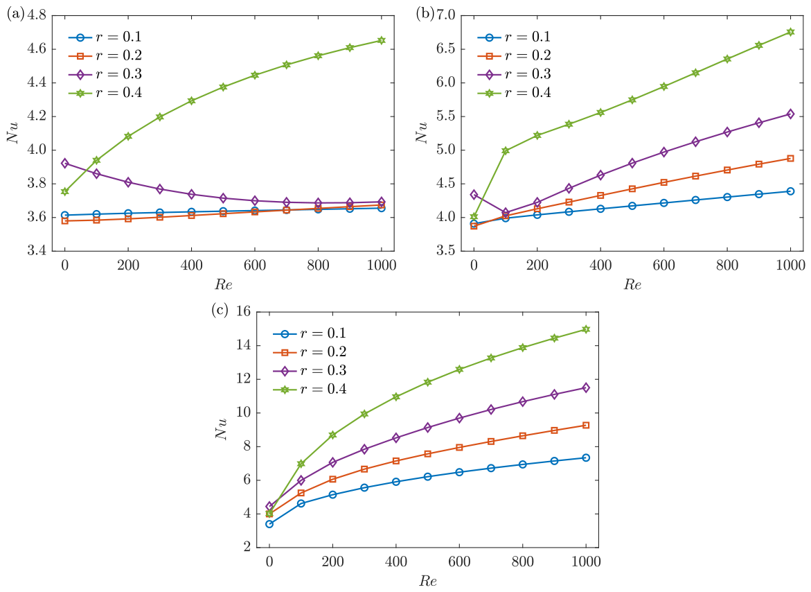
Finally, Figure 15 depicts the relationship between the Nusselt number and the Reynolds number for various values of the cylinder radius at three different Prandtl numbers. It is seen that the dependence of $Nu$ on the radius (r) is non-monotonic when the cylinder is static, and an intermediate value of $r=0.3$ results in the best heat-transport performance for all Prandtl numbers. On the other hand, as the immersed circular cylinder rotates, $Nu$ obtains its maximum value at the largest radius of $r=0.4$, which can be attributed to stronger shear and thinning of the thermal boundary layer. The enhancements of the calculated Nusselt number due to the rotation of the cylinder are $23.9\%$, $68.4\%$, and $272.2\%$ for $Pr=0.1$, $Pr=1$, and $Pr=10$, respectively, at $r=0.4$, as well as $Re=1000$. The results demonstrate that combined effects of buoyancy and shear can enhance heat-transport efficiency in the mixed Rayleigh–Bénard convection system.

Figure 15. The Nusselt number ($Nu$) as a function of the Reynolds number ($Re$) at different cylinder radii (r) for Prandtl numbers of (a) $Pr=0.1$, (b) $Pr=1$, and (c) $Pr=10$.

4. Summary and Conclusions

An immersed boundary method (IBM) for solving non-isothermal incompressible viscous flows around a rotating cylinder with convective heat transfer has been presented. The numerical integration is based on a second-order fractional step method under a staggered Cartesian grid system [54]. A modified mass source/sink term calculated at both the interface and solid cell faces is introduced into the continuity equation to ensure mass conservation for the fluid portion of the interface cells cut by the immersed boundary. Numerical tests for the flow induced by a rotating solid disk reveal that the overall second-order spatial accuracy of the base solver is preserved. To validate the accuracy of the method, forced convection over a rotating isothermal circular cylinder was simulated, and the results show good agreement with available data in the literature. Lastly, mixed Rayleigh–Bénard convection driven by buoyancy and shear forces in an annulus was investigated at a Rayleigh number of $Ra={10}^5$ for different Prandtl numbers and cylinder radii, showing that heat transport can be greatly enhanced by increasing the rotating rate under larger values of the cylinder radius. The present method has been proven to be capable of simulating heat-transfer problems in flows around rigid objects.

References

- Yan, Y.; Zu, Y. Numerical simulation of heat transfer and fluid flow past a rotating isothermal cylinder—A LBM approach. Int. J. Heat Mass Transf. 2008, 51, 2519–2536. [Google Scholar] [CrossRef] [Scilit]
- Paramane, S.B.; Sharma, A. Numerical investigation of heat and fluid flow across a rotating circular cylinder maintained at constant temperature in 2-D laminar flow regime. Int. J. Heat Mass Transf. 2009, 52, 3205–3216. [Google Scholar] [CrossRef] [Scilit]
- Panda, S.K.; Chhabra, R. Laminar forced convection heat transfer from a rotating cylinder to power-law fluids. Numer. Heat Transf. Part A Appl. 2011, 59, 297–319. [Google Scholar] [CrossRef] [Scilit]
- Sharma, V.; Dhiman, K.A. Heat transfer from a rotating circular cylinder in the steady regime: Effects of Prandtl number. Therm. Sci. 2012, 16, 79–91. [Google Scholar] [CrossRef] [Scilit]
- Yoon, H.; Seo, J.; Kim, J. Laminar forced convection heat transfer around two rotating side-by-side circular cylinder. Int. J. Heat Mass Transf. 2010, 53, 4525–4535. [Google Scholar] [CrossRef] [Scilit]
- Sufyan, M.; Manzoor, S.; Sheikh, N.A. Free stream flow and forced convection heat transfer across rotating circular cylinder in steady regime: Effects of rotation, Prandtl number and thermal boundary condition. J. Mech. Sci. Technol. 2015, 29, 1781–1797. [Google Scholar] [CrossRef] [Scilit]
- Shih, Y.C.; Khodadadi, J.; Weng, K.H.; Ahmed, A. Periodic fluid flow and heat transfer in a square cavity due to an insulated or isothermal rotating cylinder. J. Heat Transf. 2009, 131, 111701. [Google Scholar] [CrossRef] [Scilit]
- Roslan, R.; Saleh, H.; Hashim, I. Effect of rotating cylinder on heat transfer in a square enclosure filled with nanofluids. Int. J. Heat Mass Transf. 2012, 55, 7247–7256. [Google Scholar] [CrossRef] [Scilit]
- Liao, C.C.; Lin, C.A. Mixed convection of a heated rotating cylinder in a square enclosure. Int. J. Heat Mass Transf. 2014, 72, 9–22. [Google Scholar] [CrossRef] [Scilit]
- Nouri-Borujerdi, A.; Nakhchi, M. Heat transfer enhancement in annular flow with outer grooved cylinder and rotating inner cylinder: Review and experiments. Appl. Therm. Eng. 2017, 120, 257–268. [Google Scholar] [CrossRef] [Scilit]
- Arshadi, A.; Nili-Ahmadabadi, M.; Minaeian, A.; Ha, M.Y. Mixed-convection flow and heat transfer in a square enclosure around a rotating hot cylinder immersed in a Phan-Thien–Tanner viscoelastic fluid. Int. J. Heat Mass Transf. 2024, 229, 125710. [Google Scholar] [CrossRef] [Scilit]
- Bartwal, N.; Roy, S.; Vanka, S.P. Application of a high-order meshless method to study mixed convection heat transfer in a cavity with rotating circular cylinders. Comput. Fluids 2025, 303, 106868. [Google Scholar] [CrossRef] [Scilit]
- Mittal, R.; Iaccarino, G. Immersed boundary methods. Annu. Rev. Fluid Mech. 2005, 37, 239–261. [Google Scholar] [CrossRef] [Scilit]
- Griffith, B.E.; Patankar, N.A. Immersed methods for fluid–structure interaction. Annu. Rev. Fluid Mech. 2020, 52, 421–448. [Google Scholar] [CrossRef] [Scilit] [PubMed]
- Verzicco, R. Immersed boundary methods: Historical perspective and future outlook. Annu. Rev. Fluid Mech. 2023, 55, 129–155. [Google Scholar] [CrossRef] [Scilit]
- Mittal, R.; Seo, J.H. Origin and evolution of immersed boundary methods in computational fluid dynamics. Phys. Rev. Fluids 2023, 8, 100501. [Google Scholar] [CrossRef] [Scilit] [PubMed]
- Peskin, C.S. Flow patterns around heart valves: A numerical method. J. Comput. Phys. 1972, 10, 252–271. [Google Scholar] [CrossRef] [Scilit]
- Peskin, C.S. Numerical analysis of blood flow in the heart. J. Comput. Phys. 1977, 25, 220–252. [Google Scholar] [CrossRef] [Scilit]
- Goldstein, D.; Handler, R.; Sirovich, L. Modeling a no-slip flow boundary with an external force field. J. Comput. Phys. 1993, 105, 354–366. [Google Scholar] [CrossRef] [Scilit]
- Saiki, E.M.; Biringen, S. Numerical simulation of a cylinder in uniform flow: Application of a virtual boundary method. J. Comput. Phys. 1996, 123, 450–465. [Google Scholar] [CrossRef] [Scilit]
- Mohd-Yusof, J. Combined immersed-boundary/B-spline methods for simulations of flow in complex geometries. In Annual Research Briefs; Center for Turbulence Research: Stanford, CA, USA, 1997; pp. 317–327. [Google Scholar]
- Fadlun, E.A.; Verzicco, R.; Orlandi, P.; Mohd-Yusof, J. Combined immersed-boundary finite-difference methods for three-dimensional complex flow simulations. J. Comput. Phys. 2000, 161, 35–60. [Google Scholar] [CrossRef] [Scilit]
- Li, Z.; Lai, M.C. The immersed interface method for the Navier–Stokes equations with singular forces. J. Comput. Phys. 2001, 171, 822–842. [Google Scholar] [CrossRef] [Scilit]
- Xu, S.; Wang, Z.J. An immersed interface method for simulating the interaction of a fluid with moving boundaries. J. Comput. Phys. 2006, 216, 454–493. [Google Scholar] [CrossRef] [Scilit]
- Tseng, Y.H.; Ferziger, J.H. A ghost-cell immersed boundary method for flow in complex geometry. J. Comput. Phys. 2003, 192, 593–623. [Google Scholar] [CrossRef] [Scilit]
- Ghias, R.; Mittal, R.; Dong, H. A sharp interface immersed boundary method for compressible viscous flows. J. Comput. Phys. 2007, 225, 528–553. [Google Scholar] [CrossRef] [Scilit]
- Mittal, R.; Dong, H.; Bozkurttas, M.; Najjar, F.; Vargas, A.; Von Loebbecke, A. A versatile sharp interface immersed boundary method for incompressible flows with complex boundaries. J. Comput. Phys. 2008, 227, 4825–4852. [Google Scholar] [CrossRef] [Scilit] [PubMed]
- Ye, T.; Mittal, R.; Udaykumar, H.; Shyy, W. An accurate Cartesian grid method for viscous incompressible flows with complex immersed boundaries. J. Comput. Phys. 1999, 156, 209–240. [Google Scholar] [CrossRef] [Scilit]
- Udaykumar, H.; Mittal, R.; Rampunggoon, P.; Khanna, A. A sharp interface Cartesian grid method for simulating flows with complex moving boundaries. J. Comput. Phys. 2001, 174, 345–380. [Google Scholar] [CrossRef] [Scilit]
- Chung, M.H. Cartesian cut cell approach for simulating incompressible flows with rigid bodies of arbitrary shape. Comput. Fluids 2006, 35, 607–623. [Google Scholar] [CrossRef] [Scilit]
- Meinke, M.; Schneiders, L.; Günther, C.; Schröder, W. A cut-cell method for sharp moving boundaries in Cartesian grids. Comput. Fluids 2013, 85, 135–142. [Google Scholar] [CrossRef] [Scilit]
- Balaras, E. Modeling complex boundaries using an external force field on fixed Cartesian grids in large-eddy simulations. Comput. Fluids 2004, 33, 375–404. [Google Scholar] [CrossRef] [Scilit]
- Yang, J.; Balaras, E. An embedded-boundary formulation for large-eddy simulation of turbulent flows interacting with moving boundaries. J. Comput. Phys. 2006, 215, 12–40. [Google Scholar] [CrossRef] [Scilit]
- Zhang, N.; Zheng, Z. An improved direct-forcing immersed-boundary method for finite difference applications. J. Comput. Phys. 2007, 221, 250–268. [Google Scholar] [CrossRef] [Scilit]
- Yang, J.; Stern, F. A non-iterative direct forcing immersed boundary method for strongly-coupled fluid–solid interactions. J. Comput. Phys. 2015, 295, 779–804. [Google Scholar] [CrossRef] [Scilit]
- Yildiran, I.N.; Beratlis, N.; Capuano, F.; Loke, Y.H.; Squires, K.; Balaras, E. Pressure boundary conditions for immersed-boundary methods. J. Comput. Phys. 2024, 510, 113057. [Google Scholar] [CrossRef] [Scilit] [PubMed]
- Taira, K.; Colonius, T. The immersed boundary method: A projection approach. J. Comput. Phys. 2007, 225, 2118–2137. [Google Scholar] [CrossRef] [Scilit]
- Kim, J.; Kim, D.; Choi, H. An immersed-boundary finite-volume method for simulations of flow in complex geometries. J. Comput. Phys. 2001, 171, 132–150. [Google Scholar] [CrossRef] [Scilit]
- Huang, W.X.; Sung, H.J. Improvement of mass source/sink for an immersed boundary method. Int. J. Numer. Methods Fluids 2007, 53, 1659–1671. [Google Scholar] [CrossRef] [Scilit]
- Mittal, R.; Bhardwaj, R. Immersed boundary methods for thermofluids problems. Annu. Rev. Heat Transf. 2021, 24, 33–70. [Google Scholar]
- Kim, J.; Choi, H. An immersed-boundary finite-volume method for simulation of heat transfer in complex geometries. KSME Int. J. 2004, 18, 1026–1035. [Google Scholar] [CrossRef] [Scilit]
- Pacheco, J.; Pacheco-Vega, A.; Rodić, T.; Peck, R. Numerical simulations of heat transfer and fluid flow problems using an immersed-boundary finite-volume method on nonstaggered grids. Numer. Heat Transf. Part B Fundam. 2005, 48, 1–24. [Google Scholar] [CrossRef] [Scilit]
- Pan, D. An immersed boundary method on unstructured Cartesian meshes for incompressible flows with heat transfer. Numer. Heat Transf. Part B Fundam. 2006, 49, 277–297. [Google Scholar] [CrossRef] [Scilit]
- Pacheco-Vega, A.; Pacheco, J.R.; Rodić, T. A general scheme for the boundary conditions in convective and diffusive heat transfer with immersed boundary methods. J. Heat Transf. 2007, 129, 1506–1516. [Google Scholar] [CrossRef] [Scilit]
- Liao, C.C.; Lin, C.A. Simulations of natural and forced convection flows with moving embedded object using immersed boundary method. Comput. Methods Appl. Mech. Eng. 2012, 213, 58–70. [Google Scholar] [CrossRef] [Scilit]
- Xia, J.; Luo, K.; Fan, J. A ghost-cell based high-order immersed boundary method for inter-phase heat transfer simulation. Int. J. Heat Mass Transf. 2014, 75, 302–312. [Google Scholar] [CrossRef] [Scilit]
- Chern, M.J.; Noor, D.Z.; Liao, C.B.; Horng, T.L. Direct-forcing immersed boundary method for mixed heat transfer. Commun. Comput. Phys. 2015, 18, 1072–1094. [Google Scholar] [CrossRef] [Scilit]
- Yao, G. A Simple Immersed Boundary Method for Modeling Forced Convection Heat Transfer. J. Heat Transf. 2020, 142, 101802. [Google Scholar] [CrossRef] [Scilit]
- Xu, T.; Choi, J.I. Efficient monolithic immersed boundary projection method for incompressible flows with heat transfer. J. Comput. Phys. 2023, 477, 111929. [Google Scholar] [CrossRef] [Scilit]
- Zhang, N.; Zheng, Z.; Eckels, S. Study of heat-transfer on the surface of a circular cylinder in flow using an immersed-boundary method. Int. J. Heat Fluid Flow 2008, 29, 1558–1566. [Google Scholar] [CrossRef] [Scilit]
- Wang, Z.; Fan, J.; Luo, K.; Cen, K. Immersed boundary method for the simulation of flows with heat transfer. Int. J. Heat Mass Transf. 2009, 52, 4510–4518. [Google Scholar] [CrossRef] [Scilit]
- Ren, W.; Shu, C.; Yang, W. An efficient immersed boundary method for thermal flow problems with heat flux boundary conditions. Int. J. Heat Mass Transf. 2013, 64, 694–705. [Google Scholar] [CrossRef] [Scilit]
- Krasnov, D.; Zikanov, O.; Boeck, T. Comparative study of finite difference approaches in simulation of magnetohydrodynamic turbulence at low magnetic Reynolds number. Comput. Fluids 2011, 50, 46–59. [Google Scholar] [CrossRef] [Scilit]
- Zhang, Y.; Zhou, Q. Eliminating flow reversals and enhancing heat transport in turbulent thermal convection with sinusoidally heated plates. Int. J. Heat Mass Transf. 2025, 239, 126560. [Google Scholar] [CrossRef] [Scilit]
- Morinishi, Y.; Lund, T.S.; Vasilyev, O.V.; Moin, P. Fully conservative higher order finite difference schemes for incompressible flow. J. Comput. Phys. 1998, 143, 90–124. [Google Scholar] [CrossRef] [Scilit]
- Guy, R.D.; Hartenstine, D.A. On the accuracy of direct forcing immersed boundary methods with projection methods. J. Comput. Phys. 2010, 229, 2479–2496. [Google Scholar] [CrossRef] [Scilit]
- Seo, J.H.; Mittal, R. A sharp-interface immersed boundary method with improved mass conservation and reduced spurious pressure oscillations. J. Comput. Phys. 2011, 230, 7347–7363. [Google Scholar] [CrossRef] [Scilit] [PubMed]
- Lee, J.; You, D. An implicit ghost-cell immersed boundary method for simulations of moving body problems with control of spurious force oscillations. J. Comput. Phys. 2013, 233, 295–314. [Google Scholar] [CrossRef] [Scilit]
- Nicolaou, L.; Jung, S.; Zaki, T. A robust direct-forcing immersed boundary method with enhanced stability for moving body problems in curvilinear coordinates. Comput. Fluids 2015, 119, 101–114. [Google Scholar] [CrossRef] [Scilit]
- Lee, J.; Kim, J.; Choi, H.; Yang, K.S. Sources of spurious force oscillations from an immersed boundary method for moving-body problems. J. Comput. Phys. 2011, 230, 2677–2695. [Google Scholar] [CrossRef] [Scilit]
- Roache, P. Perspective: A method for uniform reporting of grid refinement studies. J. Fluids Eng. 1994, 116, 405–413. [Google Scholar] [CrossRef] [Scilit]
- Kang, S.; Choi, H.; Lee, S. Laminar flow past a rotating circular cylinder. Phys. Fluids 1999, 11, 3312–3321. [Google Scholar] [CrossRef] [Scilit]
- Jagad, P.; Mohamed, M.S.; Samtaney, R. Investigation of flow past a cylinder embedded on curved and flat surfaces. Phys. Rev. Fluids 2020, 5, 044701. [Google Scholar] [CrossRef] [Scilit]
- Berthelsen, P.A.; Faltinsen, O.M. A local directional ghost cell approach for incompressible viscous flow problems with irregular boundaries. J. Comput. Phys. 2008, 227, 4354–4397. [Google Scholar] [CrossRef] [Scilit]
- Das, S.; Panda, A.; Deen, N.; Kuipers, J. A sharp-interface immersed boundary method to simulate convective and conjugate heat transfer through highly complex periodic porous structures. Chem. Eng. Sci. 2018, 191, 1–18. [Google Scholar] [CrossRef] [Scilit]
- Badr, H.; Dennis, S. Laminar forced convection from a rotating cylinder. Int. J. Heat Mass Transf. 1985, 28, 253–264. [Google Scholar] [CrossRef] [Scilit]
- Soares, A.; Rouboa, A. Viscous dissipation in the heat transfer between a rotating cylinder and viscous media under forced convection. Energy Rep. 2021, 7, 83–97. [Google Scholar] [CrossRef] [Scilit]
- Panda, S.K.; Chhabra, R. Laminar flow of power-law fluids past a rotating cylinder. J. Non-Newton. Fluid Mech. 2010, 165, 1442–1461. [Google Scholar] [CrossRef] [Scilit]
- Luo, K.; Zhuang, Z.; Fan, J.; Haugen, N.E.L. A ghost-cell immersed boundary method for simulations of heat transfer in compressible flows under different boundary conditions. Int. J. Heat Mass Transf. 2016, 92, 708–717. [Google Scholar] [CrossRef] [Scilit]
- Mahfouz, F.; Badr, H. Forced convection from a rotationally oscillating cylinder placed in a uniform stream. Int. J. Heat Mass Transf. 2000, 43, 3093–3104. [Google Scholar] [CrossRef] [Scilit]
- Mahir, N.; Altaç, Z. Numerical investigation of convective heat transfer in unsteady flow past two cylinders in tandem arrangements. Int. J. Heat Fluid Flow 2008, 29, 1309–1318. [Google Scholar] [CrossRef] [Scilit]
- Stojković, D.; Breuer, M.; Durst, F. Effect of high rotation rates on the laminar flow around a circular cylinder. Phys. Fluids 2002, 14, 3160–3178. [Google Scholar] [CrossRef] [Scilit]
- Dalal, A.; Eswaran, V.; Biswas, G. A finite-volume method for Navier–Stokes equations on unstructured meshes. Numer. Heat Transf. Part B Fundam. 2008, 54, 238–259. [Google Scholar] [CrossRef] [Scilit]
- Hassanzadeh, R.; Rahimi, R.; Khosravipour, A.; Mostafavi, S.; Pekel, H. Analysis of natural convection in a square cavity in the presence of a rotating cylinder with a specific number of roughness components. Int. Commun. Heat Mass Transf. 2020, 116, 104708. [Google Scholar] [CrossRef] [Scilit]
- Zhang, Y.; Huang, Y.X.; Jiang, N.; Liu, Y.L.; Lu, Z.M.; Qiu, X.; Zhou, Q. Statistics of velocity and temperature fluctuations in two-dimensional Rayleigh–Bénard convection. Phys. Rev. E 2017, 96, 023105. [Google Scholar] [CrossRef] [Scilit]
- Zhang, Y.; Zhou, Q. Low-Prandtl-number effects on global and local statistics in two-dimensional Rayleigh–Bénard convection. Phys. Fluids 2024, 36, 015107. [Google Scholar] [CrossRef] [Scilit]
- Zhang, Y.; Zhou, Q.; Sun, C. Statistics of kinetic and thermal energy dissipation rates in two-dimensional turbulent Rayleigh–Bénard convection. J. Fluid Mech. 2017, 814, 165–184. [Google Scholar] [CrossRef] [Scilit]
Disclaimer/Publisher’s Note: The statements, opinions and data contained in all publications are solely those of the individual author(s) and contributor(s) and not of MDPI and/or the editor(s). MDPI and/or the editor(s) disclaim responsibility for any injury to people or property resulting from any ideas, methods, instructions or products referred to in the content. |
© 2026 by the authors. Licensee MDPI, Basel, Switzerland. This article is an open access article distributed under the terms and conditions of the Creative Commons Attribution (CC BY) license.