Unsteady Poiseuille-Type Flow of a Vinogradov–Pokrovskii Polymer Fluid in a Flat Channel: An Explicit Modal Solution and Its Convergence

Abstract

We study the unsteady mechanical response of an incompressible viscoelastic polymeric fluid in a flat channel, governed by the Vinogradov–Pokrovskii rheological model. The motion arises from an electrohydrodynamic reduction of Poiseuille type, after which the mechanical subsystem decouples from the electric field; the velocity then depends on time and on the transverse coordinate only. Treating the rheological parameter as small, we reduce the governing system in the leading-order approximation to a non-autonomous second-order evolution equation whose stiffness coefficient relaxes exponentially in time, so that the nonstationarity is driven by the internal relaxation of the normal stress rather than by an external force. For spatially homogeneous initial normal stress, we diagonalize the Galerkin system in the sine basis and obtain an explicit modal representation in which each mode satisfies a Bessel equation whose order depends on the mode number. This yields a critical index that splits the modes into three regimes—real order, zero order, and purely imaginary order—a structure absent from the classical UCM and Oldroyd-B solutions. Using the explicit representation, we prove convergence of the modal series and show that the solution decays in the long-time limit, so that the rest state is asymptotically stable in the natural energy phase space. The analytical solution is confirmed numerically.

1. Introduction

Unsteady Poiseuille-type flows in flat channels constitute one of the natural classes of problems in mathematical hydrodynamics. In the classical Newtonian case, such problems serve as a convenient model for studying the influence of a time-prescribed pressure gradient on the velocity profile, the flow rate, and the wall shear stress. For viscoelastic polymeric fluids, the unsteady problem becomes substantially more complicated, since, along with the velocity field, one must account for the evolution of the internal stresses and for the relaxation properties of the medium.

In the present work, we consider the flow of an incompressible viscoelastic polymeric fluid in a flat channel. As a mathematical basis, we use the structural–phenomenological Vinogradov–Pokrovskii model, which goes back to a mesoscopic description of the dynamics of linear polymers [1,2]. In this model, the polymeric medium is regarded as a system of macromolecular chains moving in an anisotropic surrounding fluid. The formulated physical model makes it possible to account for slow relaxation processes, normal stresses, and the internal anisotropy of the medium—effects that are not reflected in the simplest Newtonian or linear viscoelastic models. As noted in Refs. [3,4,5,6,7], the adopted physical representation of a continuous polymeric medium makes it possible to describe its main rheological properties: the decrease in the viscosity and in the first normal-stress difference toward a definite limit as the deformation rates increase.

In addition, the Vinogradov–Pokrovskii model, in contrast to other well-known models [8,9,10], makes it possible to obtain nonzero values of the second normal-stress difference. Specifically, the influence of the anisotropy of the medium surrounding a selected macromolecule is taken into account, an anisotropy caused by the stretching and orientation of the macromolecular chains forming it. The rheological properties predicted by the Vinogradov–Pokrovskii model agree qualitatively and quantitatively with experimental data for polymer solutions and melts [11,12,13].

Problems of Poiseuille-type flows for the Vinogradov–Pokrovskii model and its generalizations were studied earlier in works by A. M. Blokhin and his collaborators. In those works, steady solutions, the spectral properties of linearized problems, and the Lyapunov stability and instability of steady flows and rest states in flat and cylindrical channels were considered, including electrohydrodynamic and magnetohydrodynamic modifications of the model [5,7,14,15,16,17].

The first essential distinction of the present work concerns the nature of the nonstationarity. Unsteady Poiseuille flow is itself classical, so studying a time-dependent regime is not new in itself. What is essential here is that the nonstationarity is not prescribed externally: even when the pressure gradient is switched off, the problem remains essentially non-autonomous, because the internal normal stress relaxes exponentially and enters the stiffness coefficient of the equation for the velocity. In the works mentioned above on the Vinogradov–Pokrovskii model, the main attention was paid to steady flows, spectral asymptotics, and the linear stability or instability of steady states; here, by contrast, we derive a non-autonomous equation for the velocity generated by this internal relaxation, construct an explicit modal solution, and study its convergence and its behavior as $t\to \infty$. To the best of our knowledge, for this unsteady Poiseuille reduction of the Vinogradov–Pokrovskii model, an explicit modal representation in terms of Bessel functions and its asymptotic decay have not been investigated before.

For comparison, we note that for the classical viscoelastic models, UCM, Oldroyd-B, and their generalizations, a number of works are known in which one-dimensional unsteady flows admit an exact analytical description. In the classical work of Waters and King [18], unsteady flows of an elastico-viscous liquid were studied; this work is often regarded as one of the early sources of exact solutions for linear viscoelastic models. In the works of Hayat, Siddiqui, and Asghar [19] and Hayat, Khan, and Ayub [20], exact solutions of several simple unsteady flows of an Oldroyd-B fluid were obtained, including the Stokes problems, the modified Stokes problem, periodic Poiseuille flow, unsteady Couette flow, and unsteady Poiseuille flow. These solutions are constructed by the Laplace transform, the Fourier transform, and the corresponding series methods. In the work of Fetecau and Kannan [21], exact formulas for the velocity and the shear stress in an unsteady flow of an Oldroyd-B fluid were also obtained by the method of integral transforms. In the paper of Fetecau, Hayat, Khan, and Fetecau [22], the solution of the problem of the motion of a fluid induced by the impulsive motion of a flat wall between two side walls is represented by means of a finite Fourier sine transform; here, the solutions for the Maxwell, Newtonian, and second-grade fluids arise as limiting cases. For generalized Oldroyd-B fluids, exact solutions are usually expressed through Laplace and Fourier transforms are written by means of integrals or series, including generalized special functions [23,24]. In the work of Qi and Xu [25], for a generalized Oldroyd-B fluid with a fractional derivative, the velocity distribution between parallel plates was obtained by means of a discrete Laplace transform and a finite Fourier sine transform.

The second essential distinction of the present work consists in the fact that the known exact solutions for the UCM/Oldroyd-B models usually have a form obtained by means of integral transforms, exponential factors, and trigonometric series, and in fractional models also of Mittag–Leffler functions or generalized special functions. In the present work, after the reduction of the Vinogradov–Pokrovskii model, a different modal structure arises. The nonstationarity is determined not only by an external action or by a time-prescribed pressure gradient, but also by the relaxation of the internal normal component of the stress tensor. In the leading-order approximation, this leads to a modal equation with an exponentially decaying stiffness coefficient.

The starting point is the electrohydrodynamic system for a weakly conducting incompressible polymeric fluid. A reduction of the Poiseuille type is considered:

$$\begin{array}{c}u=u(y,t),v\equiv 0,P=\mathcal{P}(y,t)-A\left(t\right)x,\\ \mathrm{\Phi }=\mathrm{\Phi }(y,t),q=q(y,t).\end{array}$$

Under such an approach, the full system splits into two independent subsystems: the electric subsystem for the volume charge q and the electric potential $\mathrm{\Phi }$, and the mechanical subsystem for the longitudinal velocity and the components of the stress tensor. The electric subsystem, describing the unsteady distribution of the volume charge and the electric potential, was investigated numerically earlier in Ref. [26]. In the present article, we continue the study of the same Poiseuille reduction, but the main attention is paid to the mechanical subsystem, which leads to a non-autonomous equation for the longitudinal velocity.

As a small parameter, we use the parameter $\beta$ entering the rheological equations of the model. It is assumed that $\beta \ll 1$, and the solution is sought in the form of a regular asymptotic expansion. In the leading-order approximation, the mechanical subsystem reduces to a linear non-autonomous second-order equation for the longitudinal velocity $U(t,y)$. The coefficient at the highest spatial derivative is determined by the relaxation of the normal component of the stress tensor and has the form

$$k(y,t)=A_{22}(y,t)+{\varkappa }^2,A_{22}(t,y)=e^{-t/\mathrm{Wi}}{\left({\alpha }_{22}\right)}_0\left(y\right).$$

Thus, the nonstationarity of the problem is connected not only with a time-prescribed pressure gradient, but also with the internal relaxation of the polymeric medium.

In the case of a spatially homogeneous initial normal stress ${\left({\alpha }_{22}\right)}_0\left(y\right)\equiv a_0=\mathrm{const}\ge 0$, the coefficient k depends on time only. This makes it possible to diagonalize the problem in an orthonormal sine basis and to reduce it to independent non-autonomous equations for the modal coefficients. In the homogeneous case, after a standard change of the unknown, each such equation reduces to a Bessel equation.

An essential feature of the obtained representation consists of the fact that the order of the Bessel function depends on the mode number: ${\nu }_j^2=1-4{\mathrm{Wi}}^2{\varkappa }^2{\left(j\pi \right)}^2$. This dependence of the order on the mode number is the main new feature: it generates a critical number $j^{*}={\left(2\pi \mathrm{Wi}\varkappa \right)}^{-1}$, separating the modal space into three regimes—modes of real order ($j<j^{*}$), the mode of zero order ($j=j^{*}$), and modes of purely imaginary order ($j>j^{*}$). Such a three-part classification is absent from the standard one-dimensional exact solutions for the UCM and Oldroyd-B models, where the order of the Bessel function is fixed. Moreover, since ${\varkappa }^2={\mathrm{Wi}}^{-1}/\mathrm{Re}$, the position of the threshold is determined by the competition of relaxation ($\mathrm{Wi}$) and inertia ($\mathrm{Re}$): strengthening the elastic memory transfers an ever-larger part of the modes into the purely imaginary regime, oscillating in $lnt$. The modes of purely imaginary order are investigated by means of the classical properties of Bessel functions of imaginary order [27,28].

The main results of the work are as follows. First, from the mechanical subsystem of the Vinogradov–Pokrovskii model, an unsteady equation for the velocity is derived in the leading-order approximation in the parameter $\beta$, in which the time dependence is generated by the relaxing normal stress. Second, an explicit modal solution is constructed, containing three types of Bessel modes. Third, the convergence of the modal series is established, and it is proved that in the homogeneous case $F=0$—equivalently, when the pressure gradient itself relaxes as $A\left(t\right)=A\left(0\right)e^{-t/\mathrm{Wi}}$—the solution decays, so that the rest state is asymptotically stable in $H_0^1(0,1)\times L_2(0,1)$.

2. The Full Electrohydrodynamic System

2.1. Problem Statement

The system of equations of the electrohydrodynamics of a polymeric fluid with space charge, in dimensionless form, is as follows [15,26]:

$$\begin{array}{c}\hfill \mathrm{div}\mathbf{u}=u_x+v_y=0,\end{array}$$

(1)

$$\begin{array}{c}\hfill {\displaystyle \frac{d\mathbf{u}}{dt}}+\nabla P=\mathrm{div}\Pi -\sigma q\mathbf{Q},\end{array}$$

(2)

$$\begin{array}{c}\hfill {\displaystyle \frac{d{a}_{11}}{dt}}-2A_1{u}_x-2a_{12}{u}_y+L_{11}=0,\end{array}$$

(3)

$$\begin{array}{c}\hfill {\displaystyle \frac{d{a}_{12}}{dt}}-A_1{v}_x-A_2{u}_y+{\tilde{K}}_I{a}_{12}=0,\end{array}$$

(4)

$$\begin{array}{c}\hfill {\displaystyle \frac{d{a}_{22}}{dt}}-2A_2{v}_y-2a_{12}{u}_x+L_{22}=0,\end{array}$$

(5)

$$\begin{array}{c}\hfill {\displaystyle \frac{dq}{dt}}-b\mathrm{div}\left(q\mathbf{Q}\right)=0,\end{array}$$

(6)

$$\begin{array}{c}\hfill {\Delta }_{x,y}\mathrm{\Phi }=-q.\end{array}$$

(7)

Here t is time; $x,y$ are the spatial coordinates; $u,v$ are the velocity components; ${\displaystyle \frac{d}{dt}}={\displaystyle \frac{\mathsf{\partial }}{\mathsf{\partial }t}}+(\mathbf{u},\nabla )$ is the material derivative, ${\Delta }_{x,y}={\displaystyle \frac{{\mathsf{\partial }}^2}{\mathsf{\partial }{x}^2}}+{\displaystyle \frac{{\mathsf{\partial }}^2}{\mathsf{\partial }{y}^2}}$ is the Laplace operator; P is the hydrostatic pressure; $\Pi$ is the extra-stress tensor, div$\Pi ={(\mathrm{div}(\overrightarrow{{\alpha }_1}),\mathrm{div}(\overrightarrow{{\alpha }_2}))}^{\mathrm{T}}$, ${\alpha }_1={({\alpha }_{11},{\alpha }_{21})}^{\mathrm{T}}, {\alpha }_2={({\alpha }_{12},{\alpha }_{22})}^{\mathrm{T}}$, ${\alpha }_{ij}=a_{ij}/\mathrm{Re}$ are the dimensionless components of the symmetric stress tensor; $\mathbf{Q}=\nabla \mathrm{\Phi }$ is the electric-field vector; $\mathrm{\Phi }$ is the electric potential; $q>0$ is the volume charge; the parameters are $\sigma ={\displaystyle \frac{{ϵ}_0ϵV_0^2}{\rho {(u_H\widehat{l})}^2}}$, $b={\displaystyle \frac{K{V}_0}{u_H\widehat{l}}}$, where $\widehat{l}$—characteristic length (channel width), $K>0$ is the mobility of the ions, $V_0$ is dimensional value of the potential at the anode $y=1(\widehat{l})$; ${ϵ}_0$—electric constant, $ϵ$—dielectric permittivity; $\mathrm{Re}={\displaystyle \frac{\rho u_H\widehat{l}}{{\eta }_0}}$, $\mathrm{Wi}={\displaystyle \frac{{\tau }_0{u}_H}{\widehat{l}}}$, ${\varkappa }^2={\displaystyle \frac{{\mathrm{Wi}}^{-1}}{\mathrm{Re}}}$; $A_1=a_{11}+{\mathrm{Wi}}^{-1}$, $A_2=a_{22}+{\mathrm{Wi}}^{-1}$; $L_{11}=K_I{a}_{11}+\beta (a_{11}^2+a_{12}^2)$, $L_{22}=K_I{a}_{22}+\beta (a_{12}^2+a_{22}^2)$; ${\tilde{K}}_I=K_I+\beta I$, $K_I={\mathrm{Wi}}^{-1}+{\displaystyle \frac{\overline{k}}{3}}I$, $\overline{k}=k-\beta$, $I=a_{11}+a_{22}$, where $k, \beta$ are scalar phenomenological parameters characterizing contributions associated with anisotropy. At the electrodes: at $y=0,1$ the condition $\mathbf{u}=0$ holds; at $y=0$, $\mathrm{\Phi }=0$; at $y=1$, $\mathrm{\Phi }=1$ and $q=a{\mathrm{\Phi }}_y$ ($a>0$).

At the anode $y=1$, a positive charge is injected, proportional to the strength of the electric field. The ansatz under consideration is an unsteady Poiseuille-type reduction. Indeed, as in classical plane Poiseuille flow, the velocity field is unidirectional, and the pressure depends linearly on the longitudinal coordinate. Thereby, the function $A\left(t\right)$ plays the role of a time-prescribed longitudinal pressure gradient [29,30]:

$$u=u(y,t),v\equiv 0,a_{ij}=a_{ij}(y,t),i,j=1,2,$$

$$P=\mathcal{P}(y,t)-A\left(t\right)x,\mathrm{\Phi }=\mathrm{\Phi }(y,t),q=q(y,t).$$

Under the Poiseuille-type ansatz, the electric field is purely transverse,

$$\mathbf{Q}=\nabla \mathrm{\Phi }=(0,{\mathrm{\Phi }}_y),$$

so that

$$-\sigma q\mathbf{Q}=(0,-\sigma q{\mathrm{\Phi }}_y).$$

Hence, the electric body force has no longitudinal component and does not enter the x-momentum equation governing $u(y,t)$; it contributes only to the transverse pressure balance for $\mathcal{P}(y,t)$. Moreover, since $q=q(y,t)$, $v=0$, and $q_x=0$, the charge–transport equation reduces to an equation containing no mechanical variables. Therefore, system (1)–(7) splits into the longitudinal mechanical subsystem for u and ${\alpha }_{ij}$, and the electric subsystem for q and $\mathrm{\Phi }$ [26]. In the present work, only the former is considered.

2.2. Statement of the Problem

The subsystem for the velocity and the stress tensor has the form

$$\begin{array}{cc}\hfill u_t-{\left({\alpha }_{12}\right)}_y& =A\left(t\right),\hfill \end{array}$$

(8)

$$\begin{array}{cc}\hfill {\left({\alpha }_{12}\right)}_t-{\tilde{A}}_2{u}_y+{\tilde{K}}_I{\alpha }_{12}& =0,\hfill \end{array}$$

(9)

$$\begin{array}{cc}\hfill {\left({\alpha }_{11}\right)}_t-2{\alpha }_{12}{u}_y+{\tilde{K}}_I{\alpha }_{11}-\beta \mathrm{Re}\Delta & =0,\hfill \end{array}$$

(10)

$$\begin{array}{cc}\hfill {\left({\alpha }_{22}\right)}_t+{\tilde{K}}_I{\alpha }_{22}-\beta \mathrm{Re}\Delta & =0,\hfill \end{array}$$

(11)

here, ${\tilde{A}}_2={\displaystyle \frac{A_2}{\mathrm{Re}}}$ with the boundary and initial conditions

$${u|}_{y=0,1}=0,t>0;$$

$${u|}_{t=0}=u_0\left(y\right),{\alpha }_{ij}{|}_{t=0}={\left({\alpha }_{ij}\right)}_0\left(y\right).$$

Remark 1.

The reduced constitutive equations do not require boundary conditions for ${\alpha }_{ij}$ at $y=0,1$. They contain no derivatives of the stress components with respect to y and therefore define, for each fixed y, an evolution system in t with initial data ${\left({\alpha }_{ij}\right)}_0\left(y\right)$. The only spatial boundary conditions required for the reduced mechanical subsystem are the homogeneous Dirichlet conditions imposed on the velocity.

We set $\overline{k}=k-\beta =0$ and assume $0<\beta \ll 1$. The parameter $\beta$ measures the nonlinear contribution associated with molecular orientation; hence, $\beta \to 0$ describes a weak-anisotropy regime, relevant when orientation effects remain small. Since $\overline{k}=0$, one has $K_I={\mathrm{Wi}}^{-1}$ and ${\tilde{K}}_I={\mathrm{Wi}}^{-1}+\beta I$. Under the regular perturbation assumption, $a_{ij}=A_{ij}+O\left(\beta \right)$, and hence $I=a_{11}+a_{22}=A_{11}+A_{22}+O\left(\beta \right)=O\left(1\right)$. Therefore, $\beta I=O\left(\beta \right)$ and ${\tilde{K}}_I={\mathrm{Wi}}^{-1}+O\left(\beta \right)$. Consequently, ${\tilde{K}}_I$ is replaced by ${\mathrm{Wi}}^{-1}$ when the terms of order $O\left(1\right)$ are collected; the dependence on I contributes only to the first-order system.

This motivates the regular asymptotic expansions

$$\begin{array}{cc}\hfill u(y,t)& =U(y,t)+\beta V(y,t)+O\left({\beta }^2\right),\hfill \\ \hfill {\alpha }_{ij}(y,t)& =A_{ij}(y,t)+\beta B_{ij}(y,t)+O\left({\beta }^2\right),i,j=1,2.\hfill \end{array}$$

(12)

Here, U and $A_{ij}$ denote the leading-order fields, whereas V and $B_{ij}$ represent the first-order corrections induced by the nonlinear orientation effects.

Hence, at leading order in $\beta$, the coefficient ${\tilde{K}}_I$ may be replaced by ${\mathrm{Wi}}^{-1}$. Substituting expansion (12) into Equations (8)–(11) and collecting the terms of order $O\left(1\right)$, we obtain

$$\left\{\begin{array}{c}{U}_t-{\left(A_{12}\right)}_y=A\left(t\right),\hfill \\ {\left(A_{12}\right)}_t-(A_{22}+{\varkappa }^2)U_y+{\mathrm{Wi}}^{-1}{A}_{12}=0,\hfill \\ {\left(A_{11}\right)}_t-2A_{12}{U}_y+{\mathrm{Wi}}^{-1}{A}_{11}=0,\hfill \\ {\left(A_{22}\right)}_t+{\mathrm{Wi}}^{-1}{A}_{22}=0.\hfill \end{array}\right.$$

(13)

Proposition 1 (Explicit solution for $A_{22}$).

From the last equation of the system (13) it follows that

$$A_{22}(y,t)=e^{-t/\mathrm{Wi}}{\left({\alpha }_{22}\right)}_0\left(y\right).$$

(14)

The velocity component $U(y,t)$ in the leading-order system (13) satisfies the second-order equation

$$\mathcal{L}U\equiv U_{tt}-{\left(k(y,t)U_y\right)}_y+{\mathrm{Wi}}^{-1}{U}_t=F\left(t\right),$$

(15)

where we denote

$$k(y,t)=A_{22}(y,t)+{\varkappa }^2,F\left(t\right)=A^{\prime }\left(t\right)+{\mathrm{Wi}}^{-1}A\left(t\right),$$

with the conditions

$${U|}_{y=0,1}=0,U{{|}_{t=0}=\phi \left(y\right)=u_0\left(y\right),U_t|}_{t=0}=\psi \left(y\right)=A\left(0\right)+{\left({\left({\alpha }_{12}\right)}_0\right)}_y\left(y\right).$$

(16)

2.3. Existence of a Solution

Definition 1 (Generalized solution of the first mixed problem).

Let $D=(0,1)\subset \mathbb{R}$ be a one-dimensional domain, let $Q_T=D\times (0,T)$ be the space-time cylinder of height $T>0$. A function $u\in H^1\left(Q_T\right)$ is called a generalized (weak) solution of problem (15)–(16) if the following hold:

1. 

The initial condition ${u|}_{t=0}=\phi \in {\mathring{H}}^1\left(D\right)$;

2. 

The boundary condition ${u|}_{{\mathrm{\Gamma }}_T}=0$;

3. 

The integral identity

$${\int }_{Q_T}\left(k(y,t)u_y{v}_y+{\mathrm{Wi}}^{-1}{u}_{t}v-u_t{v}_t\right)dydt={\int }_D\psi vdy+{\int }_{Q_T}Fvdydt$$

(17)

for all $v\in H^1\left(Q_T\right)$ satisfying the conditions ${v|}_{D_T}=0$ and ${v|}_{{\mathrm{\Gamma }}_T}=0$.

Assumption 1.

We assume that the following conditions hold:

1. 

The condition of uniform strict hyperbolicity:

$$k(y,t)=e^{-{\mathrm{Wi}}^{-1}t}{\left({\alpha }_{22}\right)}_0\left(y\right)+{\varkappa }^2\ge k_0>0.$$

2. 

The condition of boundedness of the initial data:

$$|{\left({\alpha }_{22}\right)}_0\left(y\right)|\le {\mu }_0=\mathrm{const}\mathit{for}\mathit{all}y\in D.$$

3. 

The condition of regularity of the data:

$$\phi \in {\mathring{H}}^1\left(D\right),\psi \in L_2\left(D\right),F\in L_2\left(Q_T\right).$$

Theorem 1 (Uniqueness of the generalized solution).

Under conditions 1 and 2, problem (15) and (16) cannot have more than one generalized solution.

Proof. 

Let $u=U^{\prime }-U^{″}$ be the difference of two solutions. Then u satisfies the homogeneous integral identity with zero initial data.

For an arbitrary $b\in (0,T]$ we introduce the test function [31,32]

$$\eta (y,t)=\left\{\begin{array}{cc}0,\hfill & b\le t\le T,\hfill \\ {\displaystyle {\int }_b^{t}u(y,\tau )d\tau ,}\hfill & 0\le t<b,\hfill \end{array}\right.$$

(18)

which has the properties ${\eta }_t=u$ for $t<b$, $\eta (y,b)=0$, and $\eta \in H^1\left(Q_T\right)$. Substituting $\eta$ into the identity and integrating by parts, we arrive at the energy equality

$$\frac{1}{2}{\int }_0^1{k}_0{\left|I(y,b)\right|}^{2}dy+\frac{1}{2}{\int \int }_{Q_b}{k}_t{\left|I\right|}^{2}dydt+{\mathrm{Wi}}^{-1}{\int \int }_{Q_b}{u}^{2}dydt+\frac{1}{2}{\int }_0^1{u}^2(y,b)dy=0,$$

(19)

where $I(y,t)={\int }_0^t{u}_y(y,\theta )d\theta$ and $Q_b=D\times (0,b)$.

Case 1: ${\left({\alpha }_{22}\right)}_0\le 0$. Then $k_t\ge 0$, and all the terms in (19) are nonnegative. Their sum equals zero, so each equals zero; in particular, $u(y,b)\equiv 0$. By the arbitrariness of b we obtain $u\equiv 0$ in $Q_T$.

Case 2: ${\left({\alpha }_{22}\right)}_0>0$. Set $\mu ={sup}_{Q_T}\left|k_t\right|<\infty$. Since $k(y,0)\ge k_0>0$, we obtain

$$\begin{array}{cc}\hfill {\displaystyle \frac{1}{2}}{\parallel u(·,b)\parallel }_{L_2(0,1)}^2+{\displaystyle \frac{k_0}{2}}{\parallel I(·,b)\parallel }_{L_2(0,1)}^2& \le {\displaystyle \frac{\mu }{2}}{\int }_0^b{\parallel I(·,b)-I(·,t)\parallel }_{L_2(0,1)}^{2}dt.\hfill \end{array}$$

Using the elementary inequality

$${\parallel I(·,b)-I(·,t)\parallel }_{L_2}^2\le {2\parallel I(·,b)\parallel }_{L_2}^2+2{\parallel I(·,t)\parallel }_{L_2}^2,$$

we find

$${\displaystyle \frac{1}{2}}{\parallel u(·,b)\parallel }_{L_2}^2+{\displaystyle \frac{k_0}{2}}{\parallel I(·,b)\parallel }_{L_2}^2\le {\mu b\parallel I(·,b)\parallel }_{L_2}^2+\mu {\int }_0^b{\parallel I(·,t)\parallel }_{L_2}^{2}dt.$$

Let

$$b_0=min\left\{T,{\displaystyle \frac{k_0}{4\mu }}\right\}.$$

Then, for $0<b\le b_0$,

$$\mu b\le {\displaystyle \frac{k_0}{4}},$$

and consequently

$${\displaystyle \frac{1}{2}}{\parallel u(·,b)\parallel }_{L_2}^2+{\displaystyle \frac{k_0}{4}}{\parallel I(·,b)\parallel }_{L_2}^2\le \mu {\int }_0^b{\parallel I(·,t)\parallel }_{L_2}^{2}dt.$$

Define

$$E\left(b\right)={\displaystyle \frac{1}{2}}{\parallel u(·,b)\parallel }_{L_2(0,1)}^2+{\displaystyle \frac{k_0}{4}}{\parallel I(·,b)\parallel }_{L_2(0,1)}^2.$$

Since

$${\parallel I(·,t)\parallel }_{L_2}^2\le {\displaystyle \frac{4}{k_0}}E\left(t\right),$$

we obtain

$$E\left(b\right)\le {\displaystyle \frac{4\mu }{k_0}}{\int }_0^{b}E\left(t\right)dt.$$

Moreover, $E\left(0\right)=0$. Hence, by Gronwall’s lemma,

$$E\left(b\right)=0,0\le b\le b_0.$$

It follows that

$$u=0\mathrm{in}D\times (0,b_0).$$

To continue the argument, let $t_m=m{b}_0$ and suppose that $u=0$ on $D\times (0,t_m)$. On the next interval $[t_m,t_{m+1}]$, where

$$t_{m+1}=min\{t_m+b_0,T\},$$

we introduce the shifted auxiliary function

$$I_m(y,t)={\int }_{t_m}^t{u}_y(y,\theta )d\theta$$

and repeat the same estimate with $t_m$ as the new initial time. Since the data at $t=t_m$ are homogeneous, we obtain

$$u=0\mathrm{in}D\times (t_m,t_{m+1}).$$

After finitely many steps, the whole interval $[0,T]$ is covered. Therefore,

$$u=0\mathrm{in}{Q}_T,$$

and the generalized solution is unique.    □

Theorem 2 (Existence of a generalized solution).

Under conditions 1, 2, and 3 the problem has a generalized solution $U\in H^1\left(Q_T\right)$.

Proof. 

In view of the specific structure of the coefficient $A_{22}(y,t)=e^{-{\mathrm{Wi}}^{-1}t}{\left({\alpha }_{22}\right)}_0\left(y\right)$ and the need to work with nonsmooth initial data, we apply the Galerkin method [33,34]. We choose a countable basis ${\left\{v_k\right\}}_{k=1}^{\infty }\subset {\mathring{H}}^1(0,1)$ and denote $V_m=span\{v_1,\dots ,v_m\}$.

We seek an approximate solution of problem (15) and (16) in the form

$$U^m(y,t)={\displaystyle \sum _{k=1}^m}{c}_k^m\left(t\right)v_k\left(y\right),U^m{|}_{\mathsf{\partial }D}=0,$$

(20)

where the coefficients $c_k^m\left(t\right)$ are determined from the conditions of orthogonality of the residual to the basis functions:

$$(U_{tt}^m,v_j)+\left(k(y,t)U_y^m,{\left(v_j\right)}_y\right)+{\mathrm{Wi}}^{-1}(U_t^m,v_j)=(F,v_j),j=1,\dots ,m,$$

(21)

with the initial conditions $U^m(·,0)={\overline{\phi }}^m$, $U_t^m(·,0)={\overline{\psi }}^m$, where ${\overline{\phi }}^m,{\overline{\psi }}^m$ are the orthogonal projections of $\phi ,\psi$ onto $V_m$. Here and below $(·,·)$ denotes the scalar product in $L^2(0,1)$.

In matrix form, (21) becomes

$$M{\mathbf{c}}^{″}\left(t\right)+{\mathrm{Wi}}^{-1}M{\mathbf{c}}^{\prime }\left(t\right)+K\left(t\right)\mathbf{c}\left(t\right)=\mathbf{F}\left(t\right),$$

(22)

where $M_{jk}=(v_j,v_k)$, $K_{jk}\left(t\right)={\int }_0^{1}k(y,t){\left(v_j\right)}_y{\left(v_k\right)}_{y}dy$, $F_j\left(t\right)=(F\left(t\right),v_j)$.

Multiplying the j-th Galerkin equation by ${\left(c_j^m\right)}^{\prime }$ and summing, we obtain

$${\mathcal{E}}_m\left(\tau \right)+{\displaystyle \frac{{\mathrm{Wi}}^{-1}}{2}}{\int }_0^{\tau }{\int }_0^1{\left(U_t^m\right)}^2\le {\mathcal{E}}_m\left(0\right)+{\displaystyle \frac{\mathrm{Wi}}{2}}{\parallel F\parallel }_{L_2\left(Q_T\right)}^2,$$

where ${\mathcal{E}}_m\left(\tau \right)=\frac{1}{2}{\int }_0^1[{\left(U_t^m\right)}^2+k{\left(U_y^m\right)}^2]dy$. We obtain the uniform estimate

$${\parallel U^m\parallel }_{H^1\left(Q_T\right)}^2\le C\left({\parallel \phi \parallel }_{H^1}^2+{\parallel \psi \parallel }_{L_2}^2+{\parallel F\parallel }_{L_2\left(Q_T\right)}^2\right).$$

(23)

Owing to the uniform estimate (23), the sequence ${\left\{U^m\right\}}_{m=1}^{\infty }$ is uniformly bounded in the space $H^1\left(Q_T\right)$.    □

3. Explicit Solution and Numerical Analysis

3.1. Explicit Solution

In Ref. [14], it was shown that in steady Poiseuille flow of the Vinogradov–Pokrovskii model, the transverse normal component ${\widehat{a}}_{22}\left(y\right)$ is uniform in y. In the electrohydrodynamic problem under consideration, the pressure gradient is absent, and the motion is generated solely by the electric field; therefore, it is natural to assume that at the initial moment the component ${\left({\alpha }_{22}\right)}_0\left(y\right)$ does not inherit the spatial inhomogeneity characteristic of shear flows under a pressure drop, and may be regarded as a constant value $A_0>0$, reflecting only a possible homogeneous preliminary stretching of the macromolecules.

Assumption 2.

Let

$${\left({\alpha }_{22}\right)}_0\left(y\right)\equiv A_0=\mathrm{const}>0.$$

(24)

Then, the stiffness coefficient

$$k\left(t\right)=A_0{e}^{-t/\mathrm{Wi}}+{\varkappa }^2$$

(25)

does not depend on y. Choosing the orthonormal sine basis $v_j\left(y\right)=\sqrt{2}sin\left(j\pi y\right)$, we obtain $M=I$ and $K_{jl}\left(t\right)={\lambda }_{j}k\left(t\right){\delta }_{jl}$, where ${\lambda }_j={\left(j\pi \right)}^2$.

Under Assumption 2, in the Galerkin approximation $U^m$ of (20), the coefficients $c_j\left(t\right)$ satisfy the independent modal equations

$$c_j^{″}\left(t\right)+{\mathrm{Wi}}^{-1}{c}_j^{\prime }\left(t\right)+{\lambda }_j\left(A_0{e}^{-t/\mathrm{Wi}}+{\varkappa }^2\right)c_j\left(t\right)=F_j\left(t\right),t>0,$$

(26)

with the initial conditions

$$c_j\left(0\right)={\phi }_j,c_j^{\prime }\left(0\right)={\psi }_j,F_j\left(t\right)={(F\left(t\right),v_j)}_{L^2},$$

and $c_j^m\left(t\right)\equiv c_j\left(t\right)$ for all $m\ge j$.

Remark 2.

In the particular case $A\left(t\right)=e^{-t/\mathrm{Wi}}$, $F=0$ reflects the exponential decay of the initial polymeric stress with Weissenberg number $\mathrm{Wi}$.

Setting $c_j\left(t\right)=e^{-t/\left(2\mathrm{Wi}\right)}{u}_j\left(t\right)$ in the homogeneous Equation (26) ($F_j\equiv 0$), we obtain

$$u_j^{″}\left(t\right)+Q_j\left(t\right)u_j\left(t\right)=0,Q_j\left(t\right)={\varkappa }^2{\lambda }_j-{\displaystyle \frac{1}{4{\mathrm{Wi}}^2}}+A_0{\lambda }_j{e}^{-t/\mathrm{Wi}}.$$

(27)

The substitution

$$z_j\left(t\right)=2\mathrm{Wi}j\pi \sqrt{A_0}{e}^{-t/\left(2\mathrm{Wi}\right)}$$

reduces Equation (27) to the Bessel equation

$${\displaystyle \frac{d^2{u}_j}{d{z}_j^2}}+{\displaystyle \frac{1}{z_j}}{\displaystyle \frac{d{u}_j}{d{z}_j}}+\left(1-{\displaystyle \frac{{\nu }_j^2}{z_j^2}}\right)u_j=0,{\nu }_j^2=1-4{\mathrm{Wi}}^2{\varkappa }^2{\left(j\pi \right)}^2.$$

(28)

Lemma 1 (Fundamental system of solutions).

The solution of Equation (28) is represented in the form

$$c_j\left(t\right)=e^{-t/\left(2\mathrm{Wi}\right)}\left[C_1^{\left(j\right)}{\mathrm{\Phi }}_1^{\left(j\right)}\left(z_j\left(t\right)\right)+C_2^{\left(j\right)}{\mathrm{\Phi }}_2^{\left(j\right)}\left(z_j\left(t\right)\right)\right].$$

Denote $j^{*}={\left(2\pi \mathrm{Wi}\varkappa \right)}^{-1}$. The fundamental system of solutions of Equation (28) is given as follows:

1. 

For $j<j^{*}$: Denote ${\nu }_j=\sqrt{1-4{\mathrm{Wi}}^2{\varkappa }^2{\left(j\pi \right)}^2}\in (0,1)$. The basis solutions are Bessel functions of opposite orders:

$${\mathrm{\Phi }}_1^{\left(j\right)}\left(z\right)=J_{{\nu }_j}\left(z\right),{\mathrm{\Phi }}_2^{\left(j\right)}\left(z\right)=J_{-{\nu }_j}\left(z\right),$$

with the Wronskian $W_j^{\mathrm{I}}\left(t\right)=\mathcal{W}\{{\mathrm{\Phi }}_1^{\left(j\right)},{\mathrm{\Phi }}_2^{\left(j\right)}\}\left(t\right)=-{\displaystyle \frac{sin\left({\nu }_j\pi \right)}{\pi \mathrm{Wi}}}{e}^{-t/\mathrm{Wi}}$;

2. 

For $j>j^{*}$: Denote ${\mu }_j=\sqrt{4{\mathrm{Wi}}^2{\varkappa }^2{\left(j\pi \right)}^2-1}>0$. The basis solutions are the real and imaginary parts of the Bessel function of imaginary order $i{\mu }_j$:

$${\mathrm{\Phi }}_1^{\left(j\right)}\left(z\right)={\mathcal{J}}_{{\mu }_j}\left(z\right)=\Re \left[J_{i{\mu }_j}\left(z\right)\right],{\mathrm{\Phi }}_2^{\left(j\right)}\left(z\right)={\mathcal{Y}}_{{\mu }_j}\left(z\right)=\Im \left[J_{i{\mu }_j}\left(z\right)\right],$$

with the Wronskian $\mathcal{W}\{{\mathcal{J}}_{\mu },{\mathcal{Y}}_{\mu }\}\left(z\right)={\displaystyle \frac{sinh\left(\pi \mu \right)}{\pi z}}\ne 0$;

3. 

For $j=j^{*}\in \mathbb{N}$ (the exceptional case $2\pi \mathrm{Wi}\varkappa j^{*}=1$): the pair $\{J_0\left(z\right),Y_0\left(z\right)\}$.

Theorem 3 Explicit solution for ${\left({\alpha }_{22}\right)}_0\equiv A_0>0$).

(Let ${\left({\alpha }_{22}\right)}_0\left(y\right)\equiv A_0=\mathrm{const}>0$, $\phi \in H_0^1(0,1)$, $\psi \in L^2(0,1)$, $F=0$. Then the solution of problem (15) is represented by the series

$$\begin{array}{cc}\hfill U(y,t)& =e^{-t/\left(2\mathrm{Wi}\right)}\sum _{\begin{array}{c}j\ge 1\\ j<j^{*}\end{array}}\sqrt{2}sin\left(j\pi y\right)\{\hfill \\ \hfill & {\phi }_j·\frac{\pi }{2sin\left({\nu }_j\pi \right)}[\left(J_{-{\nu }_j}\left(z_j^0\right)+z_j^0{J}_{-{\nu }_j}^{\prime }\left(z_j^0\right)\right)J_{{\nu }_j}\left(z_j\left(t\right)\right)\hfill \\ \hfill & -\left(J_{{\nu }_j}\left(z_j^0\right)+z_j^0{J}_{{\nu }_j}^{\prime }\left(z_j^0\right)\right)J_{-{\nu }_j}\left(z_j\left(t\right)\right)]\hfill \\ \hfill & +{\psi }_j·\frac{\pi \mathrm{Wi}}{sin\left({\nu }_j\pi \right)}\left[J_{-{\nu }_j}\left(z_j^0\right)J_{{\nu }_j}\left(z_j\left(t\right)\right)-J_{{\nu }_j}\left(z_j^0\right)J_{-{\nu }_j}\left(z_j\left(t\right)\right)\right]\}\hfill \\ \hfill & +e^{-t/\left(2\mathrm{Wi}\right)}\sqrt{2}sin\left(j^{*}\pi y\right){\mathbf{1}}_{\{j^{*}\in \mathbb{N}\}}\{\hfill \end{array}$$

$$\begin{array}{cc}\hfill & {\phi }_{j^{*}}·\frac{\pi }{2}[\left(Y_0\left(z_{*}^0\right)-z_{*}^0{Y}_1\left(z_{*}^0\right)\right)J_0\left(z_{j^{*}}\left(t\right)\right)\hfill \\ \hfill & -\left(J_0\left(z_{*}^0\right)-z_{*}^0{J}_1\left(z_{*}^0\right)\right)Y_0\left(z_{j^{*}}\left(t\right)\right)]\hfill \\ \hfill & +{\psi }_{j^{*}}·\pi \mathrm{Wi}\left[Y_0\left(z_{*}^0\right)J_0\left(z_{j^{*}}\left(t\right)\right)-J_0\left(z_{*}^0\right)Y_0\left(z_{j^{*}}\left(t\right)\right)\right]\}\hfill \\ \hfill & +e^{-t/\left(2\mathrm{Wi}\right)}\sum _{j>j^{*}}\sqrt{2}sin\left(j\pi y\right)\{\hfill \\ \hfill & {\phi }_j·\frac{\pi }{sinh\left(\pi {\mu }_j\right)}[\left({\mathcal{Y}}_{{\mu }_j}\left(z_j^0\right)+z_j^0{\mathcal{Y}}_{{\mu }_j}^{\prime }\left(z_j^0\right)\right){\mathcal{J}}_{{\mu }_j}\left(z_j\left(t\right)\right)\hfill \\ \hfill & -\left({\mathcal{J}}_{{\mu }_j}\left(z_j^0\right)+z_j^0{\mathcal{J}}_{{\mu }_j}^{\prime }\left(z_j^0\right)\right){\mathcal{Y}}_{{\mu }_j}\left(z_j\left(t\right)\right)]\hfill \\ \hfill & +{\psi }_j·\frac{2\pi \mathrm{Wi}}{sinh\left(\pi {\mu }_j\right)}\left[{\mathcal{Y}}_{{\mu }_j}\left(z_j^0\right){\mathcal{J}}_{{\mu }_j}\left(z_j\left(t\right)\right)-{\mathcal{J}}_{{\mu }_j}\left(z_j^0\right){\mathcal{Y}}_{{\mu }_j}\left(z_j\left(t\right)\right)\right]\},\hfill \end{array}$$

where the coefficients are

$$z_j\left(t\right)=2\mathrm{Wi}·j\pi \sqrt{A_0}·e^{-t/\left(2\mathrm{Wi}\right)},z_j^0=z_j\left(0\right)=2\mathrm{Wi}·j\pi \sqrt{A_0},$$

$${\phi }_j=\sqrt{2}{\int }_0^1\phi \left(y\right)sin\left(j\pi y\right)dy,{\psi }_j=\sqrt{2}{\int }_0^1\psi \left(y\right)sin\left(j\pi y\right)dy.$$

Here,

$${\mathbf{1}}_{\{j^{*}\in \mathbb{N}\}}=\left\{\begin{array}{cc}1,\hfill & j^{*}\in \mathbb{N},\hfill \\ 0,\hfill & j^{*}\notin \mathbb{N}.\hfill \end{array}\right.$$

Thus, if $j^{*}\notin \mathbb{N}$, the exceptional critical-mode term is absent from the representation.

3.2. Uniform Estimates and Convergence

For the Type II modes ($j>j^{*}$), we apply the Prüfer transformation. We introduce the amplitude $R_j\left(t\right)$ and the phase ${\varphi }_j\left(t\right)$ by the relations for Equation (27)

$$u_j\left(t\right)={\displaystyle \frac{R_j\left(t\right)}{Q_j{\left(t\right)}^{1/4}}}sin{\varphi }_j\left(t\right),u_j^{\prime }\left(t\right)=R_j\left(t\right)Q_j{\left(t\right)}^{1/4}cos{\varphi }_j\left(t\right).$$

(29)

A standard computation leads to the system

$${\varphi }_j^{\prime }\left(t\right)=-Q_j{\left(t\right)}^{1/2}-\frac{1}{4}{\displaystyle \frac{Q_j^{\prime }\left(t\right)}{Q_j\left(t\right)}}sin2{\varphi }_j\left(t\right),{\displaystyle \frac{R_j^{\prime }\left(t\right)}{R_j\left(t\right)}}=\frac{1}{4}{\displaystyle \frac{Q_j^{\prime }\left(t\right)}{Q_j\left(t\right)}}cos2{\varphi }_j\left(t\right).$$

(30)

Lemma 2 (Key integral).

For all $j>j^{*}$ we have

$$I_j={\int }_0^{\infty }{\displaystyle \frac{|Q_j^{\prime }\left(s\right)|}{Q_j\left(s\right)}}ds=ln{\displaystyle \frac{Q_j\left(0\right)}{{\alpha }_j}},{\alpha }_j={\varkappa }^2{\left(j\pi \right)}^2-{\displaystyle \frac{1}{4{\mathrm{Wi}}^2}},$$

(31)

and $I_j\le \Lambda =ln\left(Q_{j_{min}}\left(0\right)/{\alpha }_{j_{min}}\right)<\infty$, where $j_{min}=\lfloor j^{*}\rfloor +1$.

Proof. 

The substitution $\tau =e^{-s/\mathrm{Wi}}$ gives

$$I_j={\int }_0^1{\displaystyle \frac{{\beta }_{j}d\tau }{{\alpha }_j+{\beta }_j\tau }}=ln{\displaystyle \frac{Q_j\left(0\right)}{{\alpha }_j}},{\beta }_j=A_0{\left(j\pi \right)}^2.$$

The ratio $Q_j\left(0\right)/{\alpha }_j$ decreases monotonically in j, whence the maximum is attained at $j=j_{min}$.    □

Theorem 4 (Estimate of the modal coefficients).

For all $j>j^{*}$ and $t\ge 0$ the estimate holds

$$\left|c_j\left(t\right)\right|\le C{e}^{-t/\left(2\mathrm{Wi}\right)}\left(\left|{\phi }_j\right|+{\displaystyle \frac{|{\psi }_j|+C_{\mathrm{Wi}}\left|{\phi }_j\right|}{j}}\right),$$

(32)

where $C_{\mathrm{Wi}}=max\{1,1/\left(2\mathrm{Wi}\right)\}$, and the constant $C>0$ does not depend on j and t.

Proof. 

From the second equation of (30) and Lemma 2:

$$\left|ln{\displaystyle \frac{R_j\left(t\right)}{R_j\left(0\right)}}\right|\le \frac{1}{4}{I}_j\le \frac{\Lambda }{4}⟹R_j\left(t\right)\le C_0{R}_j\left(0\right),C_0=e^{\Lambda /4}.$$

From the definition (29) at $t=0$ and the identity ${sin}^2+{cos}^2=1$:

$$R_j{\left(0\right)}^2=Q_j{\left(0\right)}^{1/2}{\phi }_j^2+Q_j{\left(0\right)}^{-1/2}{\left({\psi }_j+{\phi }_j/\left(2\mathrm{Wi}\right)\right)}^2.$$

Since for $j>j^{*}$ the two-sided estimates $c_1{\lambda }_j\le Q_j\left(0\right)\le c_2{\lambda }_j$ and ${\alpha }_j\ge c_{*}{j}^2$ hold, applying $\sqrt{a+b}\le \sqrt{a}+\sqrt{b}$ we obtain

$$R_j\left(0\right)\le C_3{j}^{1/2}\left|{\phi }_j\right|+C_4{\displaystyle \frac{\left|{\psi }_j\right|+C_{\mathrm{Wi}}\left|{\phi }_j\right|}{j^{1/2}}}.$$

Substitution into $\left|c_j\left(t\right)\right|=e^{-t/\left(2\mathrm{Wi}\right)}{R}_j\left(t\right)/Q_j{\left(t\right)}^{1/4}\le e^{-t/\left(2\mathrm{Wi}\right)}{C}_0{R}_j\left(0\right)/{\alpha }_j^{1/4}$ gives (32).    □

Theorem 5 (Strong convergence in ${\mathring{H}}^1(0,1)$).

Let ${\left({\alpha }_{22}\right)}_0\equiv A_0=\mathrm{const}>0$, $\phi \in {\mathring{H}}^1(0,1)$, and $\psi \in L^2(0,1)$. Then, the series

$$U(y,t)={\displaystyle \sum _{j=1}^{\infty }}{c}_j\left(t\right)\sqrt{2}sin\left(j\pi y\right)$$

(33)

converges strongly in ${\mathring{H}}^1(0,1)$ for every $t\ge 0$, and 

$${\parallel U(·,t)\parallel }_{{\mathring{H}}^1}^2={\displaystyle \sum _{j=1}^{\infty }}{\lambda }_j{\left|c_j\left(t\right)\right|}^2\le C_{\mathrm{fin}}^2+{\tilde{C}}^2{e}^{-t/\mathrm{Wi}}\left({\parallel \phi \parallel }_{{\mathring{H}}^1}^2+{\parallel \psi \parallel }_{L^2}^2\right).$$

(34)

Proof. 

We split the sum into low ($j\le j^{*}$) and high ($j>j^{*}$) modes.

For $j\le j^{*}$, the number of indices is finite; each $c_j$ is a smooth solution of the linear ODE (26), so

$$\sum _{j\le j^{*}}{\lambda }_j{\left|c_j\left(t\right)\right|}^2\le C_{\mathrm{fin}}^2<\infty .$$

(35)

For $j>j^{*}$, from Theorem 4 and the inequality ${(a+b)}^2\le 2(a^2+b^2)$:

$${\lambda }_j{\left|c_j\left(t\right)\right|}^2\le 2C^2{e}^{-t/\mathrm{Wi}}\left({\lambda }_j|{\phi }_j{|}^2+{\pi }^2\left(\right|{\psi }_j|+C_{\mathrm{Wi}}|{\phi }_j|{)}^2\right),$$

where we used ${\left(j\pi \right)}^2/j^2={\pi }^2$. Summing over $j>j^{*}$ and applying Parseval’s equality together with the Poincaré inequality ${\parallel \phi \parallel }_{L^2}^2\le {\pi }^{-2}{\parallel \phi \parallel }_{{\mathring{H}}^1}^2$, we obtain

$$\sum _{j>j^{*}}{\lambda }_j{\left|c_j\left(t\right)\right|}^2\le {\tilde{C}}^2{e}^{-t/\mathrm{Wi}}\left({\parallel \phi \parallel }_{{\mathring{H}}^1}^2+{\parallel \psi \parallel }_{L^2}^2\right).$$

(36)

Adding (35) and (36), we arrive at (34).    □

Theorem 6 (Decay of the explicit solution).

Let the conditions for the construction of the explicit modal solution hold:

$${\left({\alpha }_{22}\right)}_0\left(y\right)\equiv A_0=\mathrm{const}\ge 0,F=0,\mathrm{Wi}>0,\varkappa >0,$$

and let

$$\phi \in H_0^1(0,1),\psi \in L_2(0,1).$$

Then the explicit solution represented by the series

$$U(t,y)={\displaystyle \sum _{j=1}^{\infty }}{c}_j\left(t\right)\sqrt{2}sin\left(j\pi y\right)$$

satisfies

$${\parallel U(t,·)\parallel }_{H_0^1(0,1)}+{\parallel U_t(t,·)\parallel }_{L_2(0,1)}⟶0,t\to \infty .$$

Consequently, the zero solution of the homogeneous problem is asymptotically stable in the phase space $\mathcal{H}=H_0^1(0,1)\times L_2(0,1)$.

Proof. 

In the case $F=0$, the modal coefficients satisfy the equations

$$c_j^{″}\left(t\right)+{\mathrm{Wi}}^{-1}{c}_j^{\prime }\left(t\right)+{\lambda }_j\left(A_0{e}^{-t/\mathrm{Wi}}+{\varkappa }^2\right)c_j\left(t\right)=0,{\lambda }_j={\left(j\pi \right)}^2.$$

After the change

$$c_j\left(t\right)=e^{-t/\left(2\mathrm{Wi}\right)}{u}_j\left(t\right),z_j\left(t\right)=2\mathrm{Wi}j\pi \sqrt{A_0}{e}^{-t/\left(2\mathrm{Wi}\right)},$$

the equation for $u_j$ reduces to the Bessel equation. Since $z_j\left(t\right)\to 0$ as $t\to \infty$, the standard small-argument asymptotics of the Bessel functions imply that for each fixed j

$$c_j\left(t\right)\to 0,c_j^{\prime }\left(t\right)\to 0,t\to \infty .$$

Indeed, for $j<j^{*}$, the functions $J_{{\nu }_j}$ and $J_{-{\nu }_j}$ with $0<{\nu }_j<1$ are used, so

$$e^{-t/\left(2\mathrm{Wi}\right)}{J}_{{\nu }_j}\left(z_j\left(t\right)\right)\to 0,e^{-t/\left(2\mathrm{Wi}\right)}{J}_{-{\nu }_j}\left(z_j\left(t\right)\right)\to 0.$$

For $j=j^{*}$ the pair $J_0,Y_0$ is used; since $Y_0\left(z\right)=O\left(\right|lnz\left|\right)$ as $z\to 0$, we have $e^{-t/\left(2\mathrm{Wi}\right)}{Y}_0\left(z_j\left(t\right)\right)\to 0$. For $j>j^{*}$ the order of the Bessel function is purely imaginary, and the corresponding real solutions have boundedly oscillating behavior as functions of $ln{z}_j\left(t\right)$. Multiplication by $e^{-t/\left(2\mathrm{Wi}\right)}$ again gives convergence to zero. Hence, in all three cases $c_j\left(t\right)\to 0$, $c_j^{\prime }\left(t\right)\to 0$.

By Parseval’s equality,

$${\parallel U(t,·)\parallel }_{L_2(0,1)}^2={\displaystyle \sum _{j=1}^{\infty }}|c_j{\left(t\right)|}^2,\parallel U_y{(t,·)\parallel }_{L_2(0,1)}^2={\displaystyle \sum _{j=1}^{\infty }}{\lambda }_j|c_j{\left(t\right)|}^2,\parallel U_t{(t,·)\parallel }_{L_2(0,1)}^2={\displaystyle \sum _{j=1}^{\infty }}{\left|c_j^{\prime }\left(t\right)\right|}^2.$$

Using the convergence estimates of the modal series obtained above and passing to the limit under the summation sign, we obtain

$${\displaystyle \sum _{j=1}^{\infty }}{\lambda }_j|c_j{\left(t\right)|}^2\to 0,{\displaystyle \sum _{j=1}^{\infty }}{\left|c_j^{\prime }\left(t\right)\right|}^2\to 0.$$

Consequently, ${\parallel U(t,·)\parallel }_{H_0^1(0,1)}+{\parallel U_t(t,·)\parallel }_{L_2(0,1)}\to 0$ as $t\to \infty$.    □

3.3. Numerical Analysis

In this subsection, we present numerical illustrations of the explicit modal solution and its comparison with the numerical solution of the truncated system of modal equations. Throughout this subsection, we fix the Weissenberg number $\mathrm{Wi}=1$, the Reynolds number $\mathrm{Re}=400$ (so that ${\varkappa }^2={\mathrm{Wi}}^{-1}/\mathrm{Re}=2.5·{10}^{-3}$), and the homogeneous initial normal stress $A_0=1$. With these values, the critical index equals $j^{*}={\left(2\pi \mathrm{Wi}\varkappa \right)}^{-1}\approx 3.18$, so that the modes $j=1,2,3$ are of real order and the modes $j\ge 4$ are of purely imaginary order; this makes the three-regime structure of the explicit solution clearly visible.

For the numerical evaluation of the modes of purely imaginary order, the complex-order Bessel function $J_{i{\mu }_j}\left(z\right)$ was computed directly using the arbitrary-precision Python library mpmath, with 25 decimal digits of working precision. The real-valued basis functions were then obtained as

$${\mathcal{J}}_{{\mu }_j}\left(z\right)=\Re J_{i{\mu }_j}\left(z\right),{\mathcal{Y}}_{{\mu }_j}\left(z\right)=\Im J_{i{\mu }_j}\left(z\right).$$

The derivatives were evaluated from the recurrence relation

$$J_{\nu }^{\prime }\left(z\right)={\displaystyle \frac{1}{2}}\left[J_{\nu -1}\left(z\right)-J_{\nu +1}\left(z\right)\right],$$

rather than by finite differences. The constants in the modal representation were determined by solving the corresponding $2\times 2$ linear system with the arbitrary-precision LU solver provided by mpmath. The resulting explicit modal solutions were also checked against an independent numerical integration of the original modal equations using the adaptive DOP853 method implemented in SciPy.

The choice of the initial profile is not arbitrary. In contrast to the symmetric Poiseuille profile, here we deliberately take an asymmetric, off-center initial datum together with a nonzero initial velocity rate, so that both the $\phi$-branch and the $\psi$-branch of the explicit representation of Theorem 3 are exercised. As the initial velocity, we use a smooth off-center bump that vanishes at the walls,

$$\phi \left(y\right)={\mathcal{N}}^{-1}\left[e^{-{(y-y_0)}^2/\left(2w^2\right)}-e^{-y_0^2/\left(2w^2\right)}(1-y)-e^{-{(1-y_0)}^2/\left(2w^2\right)}y\right],y_0=0.35,w=0.18,$$

normalized by $\mathcal{N}$ to unit peak amplitude, together with the nonzero initial rate

$$\psi \left(y\right)=0.8sin\left(\pi y\right).$$

Both $\phi$ and $\psi$ satisfy the no-slip conditions $\phi \left(0\right)=\phi \left(1\right)=0$, $\psi \left(0\right)=\psi \left(1\right)=0$, and are smooth, so that the sine coefficients

$${\phi }_j=\sqrt{2}{\int }_0^1\phi \left(y\right)sin\left(j\pi y\right)dy,{\psi }_j=\sqrt{2}{\int }_0^1\psi \left(y\right)sin\left(j\pi y\right)dy$$

decay rapidly, and the modal series converges well. The numerical reference solution is obtained by integrating the truncated modal system (26) (with $F=0$) for $j=1,\dots ,J$ with $J=60$ by a high-accuracy Runge–Kutta scheme, while the explicit solution is evaluated from Theorem 3, the modes of purely imaginary order being computed through the real and imaginary parts of the Bessel function of imaginary order $J_{i{\mu }_j}$.

1.

Evolution of the centerline velocity.

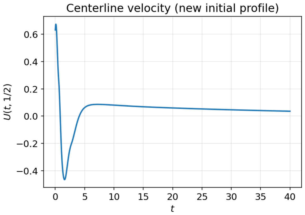
Figure 1 shows the dependence of the centerline velocity $U(t,1/2)$ on time over the interval $0\le t\le 40$. After an initial transient—in which the asymmetric profile produces a pronounced undershoot—the velocity relaxes monotonically to zero, in agreement with Theorem 6. The long time interval makes it possible to observe the decay of the solution to the rest state.

2.

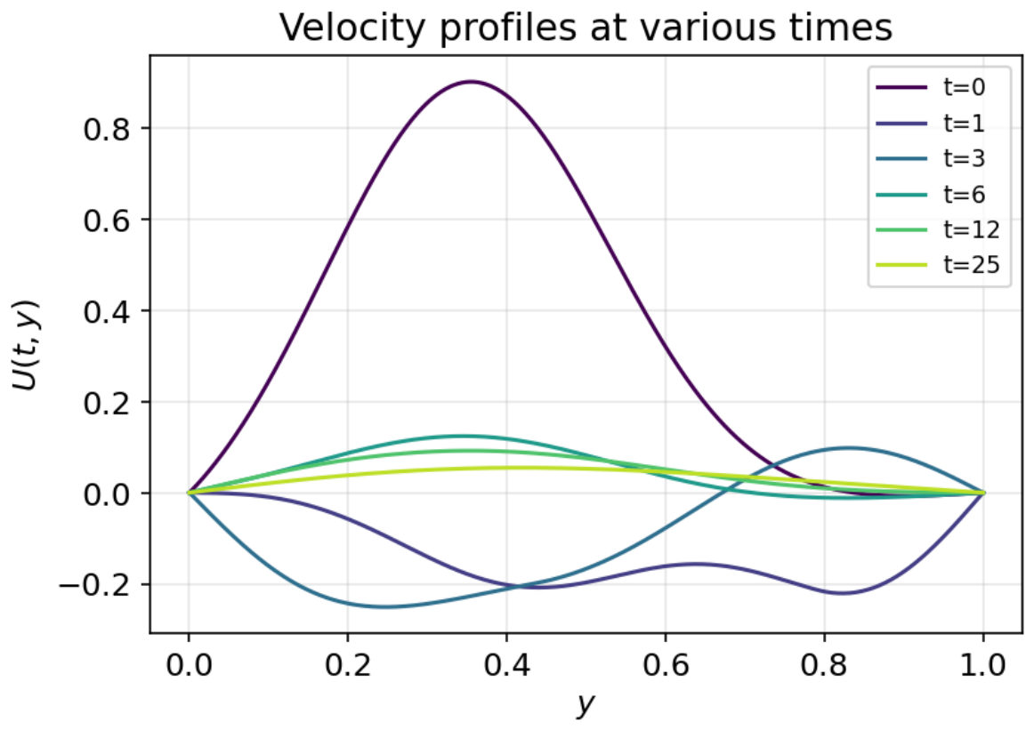
Velocity profiles at various time instants.

Figure 2 shows the profiles $U(t,y)$ at various time instants. They show how the asymmetric initial profile first redistributes across the channel—losing its initial spatial bias—and then decays uniformly to zero owing to damping and the relaxation of the internal stress.

3.

Comparison of the explicit and numerical solutions.

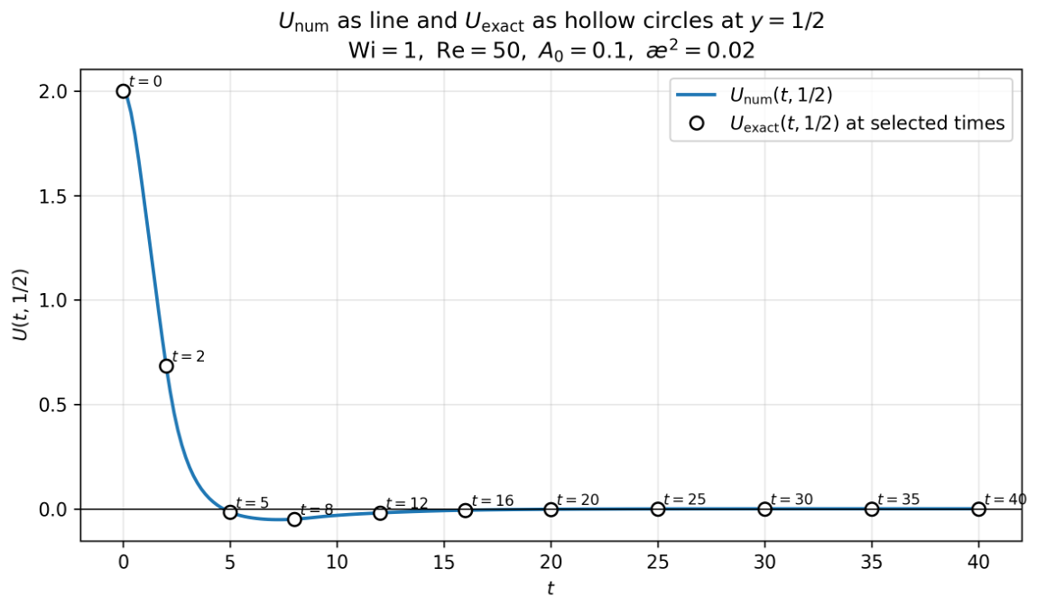
In Figure 3, the numerical solution is shown by a solid line, and the values of the explicit solution at selected time instants are shown by open circles. The two coincide in plotting accuracy, emphasizing the agreement of the numerical integration of the truncated modal system with the explicit Bessel solution.

4.

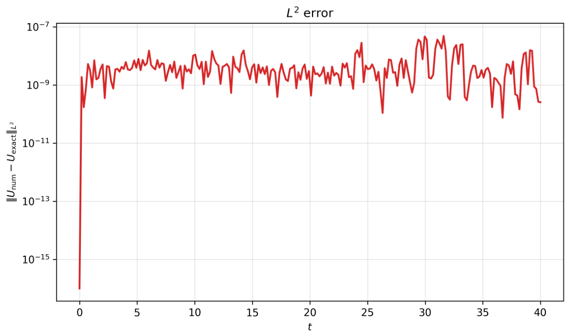
Error of the numerical solution.

Figure 4 shows the quantity $\parallel U_{\mathrm{num}}(t,·)-U_{\mathrm{exact}}{(t,·)\parallel }_{L^2(0,1)}$. The error remains at the level of the integration tolerance ($\sim {10}^{-11}$) for all t, which confirms that the numerical scheme reproduces the analytical dynamics of the solution and, conversely, that the explicit Bessel representation is correct, including the modes of purely imaginary order.

5.

Comparison of modes of real and purely imaginary order.

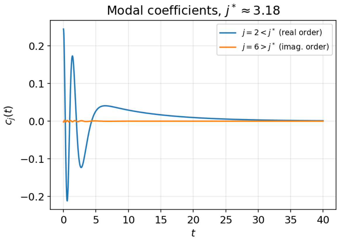
To verify the obtained modal classification, a separate modal test is carried out. Two numbers $j_{-}=2$ and $j_{+}=6$ are chosen so that $j_{-}<j^{*}$, $j_{+}>j^{*}$. The first mode corresponds to a real order of the Bessel function, and the second to a purely imaginary order. Figure 5 shows the difference in the temporal evolution of these modal coefficients: the real-order mode carries the bulk of the energy and exhibits a slow, predominantly monotone relaxation, while the imaginary-order mode is small in amplitude and decays through faster oscillations in $lnt$.

6.

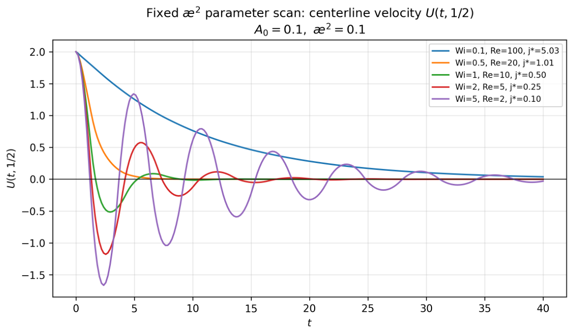
Influence of the Weissenberg number.

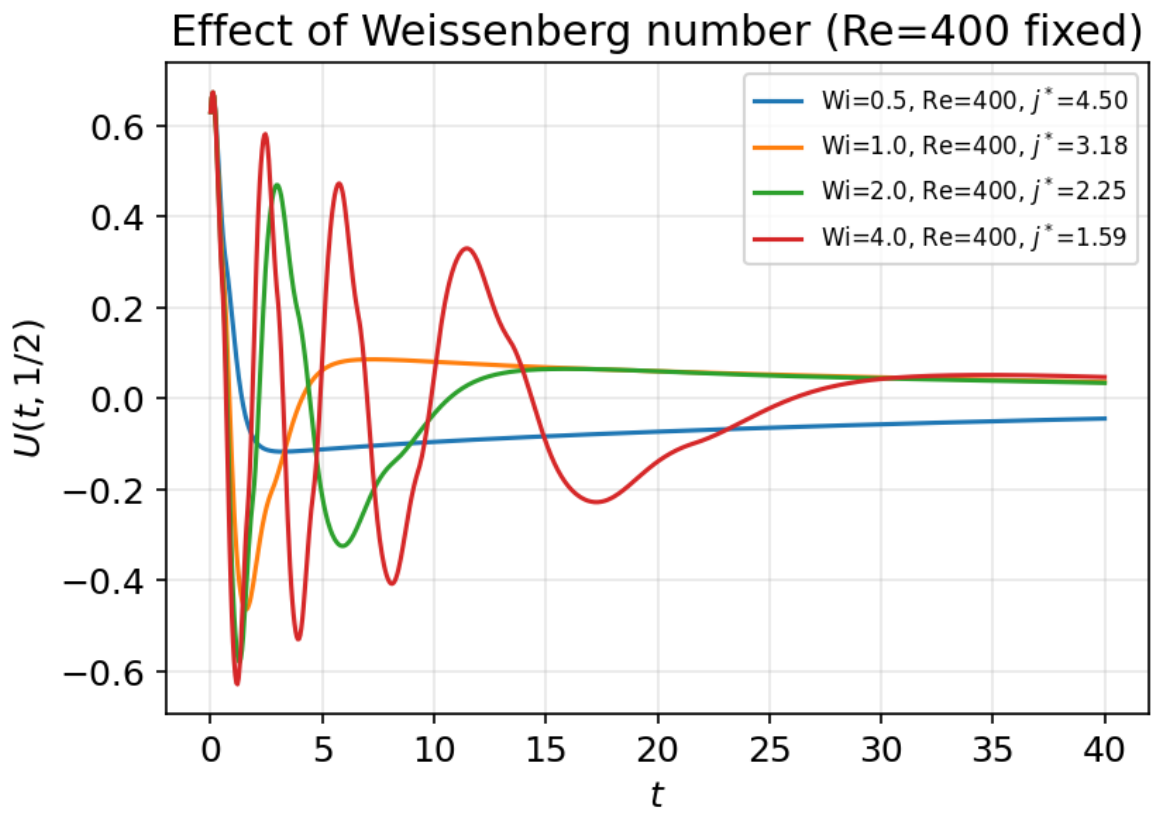
Figure 6 shows a comparison of the centerline velocity $U(t,1/2)$ for various values of the Weissenberg number $\mathrm{Wi}$ at a fixed Reynolds number $\mathrm{Re}=400$. The legend indicates the corresponding values of $\mathrm{Wi}$, $\mathrm{Re}$, and the critical number $j^{*}$. An increase in $\mathrm{Wi}$ lowers the threshold $j^{*}$, transfers more harmonics into the oscillatory imaginary-order regime, and leads to slower, more strongly oscillating decay, which corresponds to a strengthening of the viscoelastic memory.

Additionally, Figure 7 presents a series of computations at a fixed value ${\varkappa }^2=2.5·{10}^{-3}$. In this case, the influence of $\mathrm{Wi}$ is interpreted primarily as a change in the relaxation scale, while the coefficient at the spatial derivative is fixed. The legend also indicates the values of $\mathrm{Re}$ and $j^{*}$ corresponding to each $\mathrm{Wi}$.

Thus, the numerical experiments have two aims. The first is to verify the explicit solution and the numerical implementation on a nontrivial, asymmetric initial profile that activates both branches of the explicit representation. The second is to demonstrate the specific modal structure of the model under consideration: the presence of the critical number $j^{*}$ leads to different types of evolution of the low and high modes, which does not arise in the standard one-dimensional exact solutions for the UCM and Oldroyd-B models.

4. Conclusions

In this work, an unsteady Poiseuille-type problem for the Vinogradov–Pokrovskii model was considered, and in the leading-order approximation in $\beta$ a non-autonomous equation for the velocity was derived, whose stiffness coefficient relaxes through the internal normal stress. In the case of a spatially homogeneous initial normal stress ${\left({\alpha }_{22}\right)}_0\equiv a_0=\mathrm{const}\ge 0$, an explicit modal solution of the unsteady problem was obtained, whose modal coefficients are expressed through Bessel functions.

Second, the explicit solution reveals a modal structure specific to this model. After a change of the unknown, each mode satisfies a Bessel equation whose order depends on the mode number, ${\nu }_j^2=1-4{\mathrm{Wi}}^2{\varkappa }^2{\left(j\pi \right)}^2$, with the critical number $j^{*}={\left(2\pi \mathrm{Wi}\varkappa \right)}^{-1}$, separating the modal space into three regimes: real order ($j<j^{*}$), zero order ($j=j^{*}$), and purely imaginary order ($j>j^{*}$). Since $j^{*}={\left(2\pi \mathrm{Wi}\varkappa \right)}^{-1}$, an increase in the Weissenberg number lowers the threshold and transfers an ever-larger part of the modal space into the purely imaginary regime: the stronger the elastic memory, the more harmonics decay in an oscillating rather than a monotone manner.

On the basis of the explicit representation, the convergence of the modal series in ${\mathring{H}}^1(0,1)$ was established with separate uniform estimates for the low ($j<j^{*}$) and high ($j>j^{*}$) modes, and it was proved that in the homogeneous case $F=0$, the solution decays as $t\to \infty$. Consequently, the zero solution (the rest state) is asymptotically stable in the phase space $\mathcal{H}=H_0^1(0,1)\times L_2(0,1)$. We emphasize that the oscillating behavior of the high modes is compatible with this stability: the modes of purely imaginary order oscillate, but nevertheless decay, so that the whole solution tends to zero.

As a natural continuation of the present work, we plan to study the first-order perturbation terms $V(y,t)$ and $B_{ij}(y,t)$ in the expansion with respect to $\beta$. The resulting system remains linear but becomes nonhomogeneous, with source terms determined by the explicit leading-order solution obtained here. This close structural relationship with the zero-order problem suggests that similar methods may be used to investigate the existence, uniqueness, and long-time behavior of the first-order approximation, thereby clarifying the influence of the rheological parameter $\beta$.

The explicit Bessel-function solution derived in this paper may also serve as a benchmark for the verification of numerical methods. A promising direction is the construction of stable finite-difference or spectral schemes for the full EHD system, using the analytical estimates obtained here as stability and accuracy criteria.

References

1. Pokrovskii, V.N. The Mesoscopic Theory of Polymer Dynamics; Springer: Dordrecht, The Netherlands, 2010. [Google Scholar]
2. Altukhov, Y.A.; Gusev, A.S.; Pyshnograi, G.V.; Koshelev, K.B. Introduction to the Mesoscopic Theory of Fluid Polymer Systems; AltGPA: Barnaul, Russia, 2012. (In Russian) [Google Scholar]
3. Blokhin, A.M.; Tkachev, D.L. Linear asymptotic instability of a stationary flow of a polymeric medium in a plane channel in the case of periodic perturbations. J. Appl. Ind. Math. 2014, 8, 467–478. [Google Scholar] [CrossRef] [Scilit]
4. Blokhin, A.M.; Yegitov, A.V.; Tkachev, D.L. Asymptotics of the spectrum of a linearized problem of the stability of a stationary flow of an incompressible polymer fluid with a space charge. Comput. Math. Math. Phys. 2018, 58, 102–117. [Google Scholar] [CrossRef] [Scilit]
5. Blokhin, A.M.; Tkachev, D.L. Stability of Poiseuille-type flows for an MHD model of an incompressible polymeric fluid. Eur. J. Mech. B/Fluids 2020, 80, 112–120. [Google Scholar] [CrossRef] [Scilit]
6. Blokhin, A.M.; Semisalov, B.V. Finding steady Poiseuille-type flows for incompressible polymeric fluids by the relaxation method. Comput. Math. Math. Phys. 2022, 62, 302–315. [Google Scholar] [CrossRef] [Scilit]
7. Tkachev, D.L. The spectrum and Lyapunov linear instability of the stationary state for polymer fluid flows: The Vinogradov–Pokrovskii model. Sib. Math. J. 2023, 64, 407–423. [Google Scholar] [CrossRef] [Scilit]
8. Bird, R.B.; Dotson, P.J.; Johnson, N.L. Polymer solution rheology based on a finitely extensible bead-spring chain model. J. Non-Newton. Fluid Mech. 1980, 7, 213–235. [Google Scholar] [CrossRef] [Scilit]
9. Chilcott, M.D.; Rallison, J.M. Creeping flow of dilute polymer solutions past cylinders and spheres. J. Non-Newton. Fluid Mech. 1988, 29, 381–432. [Google Scholar] [CrossRef] [Scilit]
10. Remmelgas, J.; Harrison, G.; Leal, L.G. A differential constitutive equation for entangled polymer solutions. J. Non-Newton. Fluid Mech. 1999, 80, 115–134. [Google Scholar] [CrossRef] [Scilit]
11. Pokrovsky, V.N. Statistical Mechanics of Dilute Suspensions; Nauka: Moscow, Russia, 1978. (In Russian) [Google Scholar]
12. Golovicheva, I.E.; Zinovich, S.A.; Pyshnograi, G.V. Effect of the molecular mass on the shear and longitudinal viscosity of linear polymers. J. Appl. Mech. Tech. Phys. 2000, 41, 347–352. [Google Scholar] [CrossRef] [Scilit]
13. Pyshnograi, G.; Merzlikina, D.; Filip, P.; Pivokonsky, R. Mesoscopic single and multi-mode rheological models for polymeric melts viscometric flows description. WSEAS Trans. Heat Mass Transf. 2018, 13, 49–65. [Google Scholar]
14. Bambaeva, N.V.; Blokhin, A.M. Stationary solutions of Poiseuille and Couette type for equations of incompressible viscoelastic polymer fluid. J. Appl. Ind. Math. 2014, 8, 1–10. [Google Scholar]
15. Blokhin, A.M.; Rudometova, A.S. Stationary solutions of the equations for nonisothermal electroconvection of a weakly conducting incompressible polymeric liquid. J. Appl. Ind. Math. 2015, 9, 147–156. [Google Scholar] [CrossRef] [Scilit]
16. Blokhin, A.M.; Tkachev, D.L. Lyapunov instability of stationary flows of a polymeric fluid in a channel with perforated walls. Sb. Math. 2022, 213, 283–299. [Google Scholar] [CrossRef] [Scilit]
17. Blokhin, A.M.; Tkachev, D.L.; Yegitov, A.V. Lyapunov instability of the stationary flows of a polymeric fluid in an infinite plane channel with constant flow rate. J. Math. Anal. Appl. 2022, 506, 125541. [Google Scholar] [CrossRef] [Scilit]
18. Waters, N.D.; King, M.J. Unsteady flow of an elastico-viscous liquid. Rheol. Acta 1970, 9, 345–355. [Google Scholar] [CrossRef] [Scilit]
19. Hayat, T.; Siddiqui, A.M.; Asghar, S. Some simple flows of an Oldroyd-B fluid. Int. J. Eng. Sci. 2001, 39, 135–147. [Google Scholar] [CrossRef] [Scilit]
20. Hayat, T.; Khan, M.; Ayub, M. Exact solutions of flow problems of an Oldroyd-B fluid. Appl. Math. Comput. 2004, 151, 105–119. [Google Scholar] [CrossRef] [Scilit]
21. Fetecau, C.; Kannan, K. A note on an unsteady flow of an Oldroyd-B fluid. Int. J. Math. Math. Sci. 2005, 2005, 3185–3194. [Google Scholar] [CrossRef] [Scilit]
22. Fetecau, C.; Hayat, T.; Khan, M.; Fetecau, C. Unsteady flow of an Oldroyd-B fluid induced by the impulsive motion of a plate between two side walls perpendicular to the plate. Acta Mech. 2008, 198, 21–33. [Google Scholar] [CrossRef] [Scilit]
23. Fetecau, C.; Fetecau, C.; Kamran, M.; Vieru, D. Exact solutions for the flow of a generalized Oldroyd-B fluid induced by a constantly accelerating plate between two side walls perpendicular to the plate. J. Non-Newton. Fluid Mech. 2009, 156, 189–201. [Google Scholar] [CrossRef] [Scilit]
24. Fetecau, C.; Khan, M.; Fetecau, C.; Qi, H. Exact solutions for the flow of a generalized Oldroyd-B fluid induced by a suddenly moved plate between two side walls perpendicular to the plate. Proc. Romanian Acad. Ser. A 2010, 11, 3–10. [Google Scholar]
25. Qi, H.; Xu, M. Some unsteady unidirectional flows of a generalized Oldroyd-B fluid with fractional derivative. Appl. Math. Model. 2009, 33, 4184–4191. [Google Scholar] [CrossRef] [Scilit]
26. Mishchenko, E.V.; Guan, S. On the numerical determination of the volume charge and the electric potential in unsteady EHD flows of incompressible polymeric fluids. Her. Tver State Univ. Ser. Appl. Math. 2025, 1, 33–50. (In Russian) [Google Scholar]
27. Dunster, T.M. Bessel functions of purely imaginary order, with an application to second-order linear differential equations having a large parameter. SIAM J. Math. Anal. 1990, 21, 995–1018. [Google Scholar] [CrossRef] [Scilit]
28. NIST Digital Library of Mathematical Functions. Chapter 10: Bessel Functions, Section 10.24, Functions of Imaginary Order. Available online: https://dlmf.nist.gov/10.24 (accessed on 1 January 2026).
29. Galdi, G.P.; Robertson, A.M. The relation between flow rate and axial pressure gradient for time-periodic Poiseuille flow in a pipe. J. Math. Fluid Mech. 2005, 7, 215–223. [Google Scholar] [CrossRef] [Scilit]
30. Galdi, G.P.; Grobbelaar-Van Dalsen, M.; Sauer, N. Existence and uniqueness of solutions of the equations of motion for a fluid of second grade with non-homogeneous boundary conditions. Int. J. Non-Linear Mech. 1995, 30, 701–709. [Google Scholar] [CrossRef] [Scilit]
31. Ladyzhenskaya, O.A. The Boundary Value Problems of Mathematical Physics; Nauka: Moscow, Russia, 1973. (In Russian) [Google Scholar]
32. Uchida, S. The pulsating viscous flow superposed on the steady laminar motion of incompressible fluid in a circular pipe. Z. Angew. Math. Phys. 1956, 7, 403–422. [Google Scholar] [CrossRef] [Scilit]
33. Mikhailov, V.P. Partial Differential Equations; Nauka: Moscow, Russia, 1978. (In Russian) [Google Scholar]
34. Evans, L.C. Partial Differential Equations, 2nd ed.; American Mathematical Society: Providence, RI, USA, 2022; Volume 19. [Google Scholar]
Figure 1. Dependence of the centerline velocity U ( t , 1 / 2 ) on time for the asymmetric off-center initial profile ( Wi = 1 , Re = 400 , A 0 = 1 ).
Fluids 11 00184 g001
Figure 2. Velocity profiles U ( t , y ) at various time instants for the asymmetric off-center initial profile.
Fluids 11 00184 g002
Figure 3. Comparison of the numerical and explicit solutions for the centerline velocity U ( t , 1 / 2 ) : solid line—numerical solution; open circles—explicit solution.
Fluids 11 00184 g003
Figure 4. The L 2 -error between the numerical and explicit solutions.
Fluids 11 00184 g004
Figure 5. Comparison of the modal coefficients for the regimes j < j * and j > j * ( j * 3.18 ).
Fluids 11 00184 g005
Figure 6. Influence of the Weissenberg number on the centerline velocity U ( t , 1 / 2 ) at fixed Re = 400 .
Fluids 11 00184 g006
Figure 7. Influence of the Weissenberg number on the centerline velocity U ( t , 1 / 2 ) at fixed ϰ 2 = 2.5 · 10 3 .
Fluids 11 00184 g007
Disclaimer/Publisher’s Note: The statements, opinions and data contained in all publications are solely those of the individual author(s) and contributor(s) and not of MDPI and/or the editor(s). MDPI and/or the editor(s) disclaim responsibility for any injury to people or property resulting from any ideas, methods, instructions or products referred to in the content.