


Abstract
The Korteweg–de Vries (KdV) equation is widely known as a canonical model for weakly nonlinear and weakly dispersive waves, notably and historically for water waves in shallow depths. Being integrable, it has a rich solution set of interacting solitary and periodic waves. Recently, we extended it with several forcing/friction terms to describe the evolution of wind-driven water wave packets in shallow water. The outcome is a modified KdV–Burgers equation, whose relevant solutions are principally solitary wave trains forming a soliton gas. In this article that is extended further by allowing the water depth to be slowly spatially varying, and introducing a basic horizontal current, also slowly spatially varying. The outcome is a modified KdV–Burgers equation with spatially slowly varying coefficients. We adapt the Whitham modulation theory for a slowly varying solitary wave train, allowing for the prediction of wave amplitude growth/decay due to a combination of the slowly varying background and the forcing/friction terms. Numerical simulations using a Fourier spectral method are performed to exhibit and validate the modulation theory.
1. Introduction
For weakly nonlinear long water waves in shallow depths, it is widely accepted that the basic model for their description is the Korteweg–de Vries (KdV) equation. When the bottom topography varies, this leads to a variable-coefficient KdV equation, see Grimshaw [1], Grimshaw and Liu [2], Johnson [3,4] amongst many similar papers, and Craig et al. [5] for the relatively less studied case of random bottom topography. Recently in Maleewong and Grimshaw [6] (hereafter denoted as MG24) we extended this model to shallow water waves forced by wind, leading to a KdV–Burgers type of equation. In Maleewong and Grimshaw [7] this was further extended to the well-known Kadometsev–Petviashvili (KP) equation to account for horizontal two-dimensional dispersion. It is a bit surprising that applications of KdV dynamics to wind-driven waves are relatively sparse, but we note the important recent exception by Costa et al. [8] who used multi-soliton dynamics to analyse wind wave data in a shallow bay. That analysis was based on the theory of a soliton gas, see El [9] for a recent review which touches on the water wave application.
However, often wind waves propagate through regions of horizontally variable hydrology, background currents and over variable bottom topography. Hence, a variable-coefficient Korteweg–de Vries (vKdV) equation is needed to model these waves. For water and internal waves a detailed derivation was given by Grimshaw [1], Zhou and Grimshaw [10], see Section 2 for a brief outline. The outcome when wind forcing is included is, a variable-coefficient KdV–Burgers (vKdV) equation,
Here is the amplitude of the wave at the free surface, are space and time variables, is the linear long wave speed, and is the linear magnification factor, defined so that is proportional to the wave action flux density for linear long waves. The coefficients are slowly-varying functions of x, determined by the waveguide properties. The three terms in are wave growth due to a critical level instability in the wind shear profile, introduced by Miles [11], a representation of wind-induced turbulent wave stress, and a representation of turbulent bottom stress, see MG24 for the derivation, and expressions for the coefficients ; these are presented here at the end of Section 2 in Equation (33).
The vKdV Equation (1) (without wind forcing) was originally derived by Grimshaw [1] for a density-stratified fluid; for convenience, there is a brief summary here in Section 2. This derivation uses the usual KdV balance that the amplitude has the same small order as the long wave dispersion. That is has the same order of magnitude as , and in addition assumes that the waveguide properties (the coefficients ) vary slowly so that, for instance, and have the same order of magnitude. The first two terms in (1) are the dominant terms, and hence we make the transformation,
Substitution into (1) yields, to the same order of asymptotic approximation as in the derivation of (1),
The coefficients are functions of the time-like variable . Since we can assume that without loss of generality, we make a further transformation yielding the canonical form,
A further transformation yields the final form suitable for modulation analysis and numerical simulation,
The scaling factor R depends only on T and is a cumulative measure of the coefficient . The forcing coefficients are given by , . Each is a small parameter, facilitating the asymptotic analysis of Section 3.
There are two conservation equations, that for mass is (8) and that for wave action,
These lead to the global laws, assuming that as ,
for mass and wave action flux respectively. cause growth and causes decay.
In Section 2, we review the derivation of the vKdV equation, given in Grimshaw [1] for a density stratified fluid, and applied here for wind-generated water waves. In Section 3, we present a theory for modulated waves, first for cnoidal waves in Section 3.1, and then emphasising the solitary wave train limit in Section 3.2. Our numerical simulations are presented in Section 4 using initial conditions similar to those in MG24. Three initial conditions are considered. In Section 4.1, the initial condition is a solitary wave, and the simulations explore how this deforms in a variable background and under wind forcing and bottom stress. Section 4.2 examines the transition of a long-wave perturbation to a deforming solitary wave train. The stability of this is examined in Section 4.3. We conclude in Section 5 with a summary and discussion.
2. Variable-Coefficient Korteweg–de Vries Equation
The KdV equation for water waves on a constant depth and X-independent shear flow, in the absence of wind forcing was first derived by Freeman and Johnson [12] and then by many others. The derivation of the vKdV Equation (1) (again without wind forcing) was given for a density stratified fluid by Grimshaw [1], see also Grimshaw and Liu [2], Liu et al. [13,14], and is briefly reproduced here when the water density is a constant. We assume a basic state defined in . The undisturbed depth , and the free surface displacement is . The background horizontal current is with a vertical velocity field , and a corresponding pressure field which absorbs the constant water density. This basic state satisfies the full steady-state Euler equations, where the momentum equations have body forces .
each holding in the fluid domain . The boundary conditions are
An important issue here is that the specified horizontal variation of these basic fields may not be contained within the inviscid Euler equations. Hence the terms are then needed to support this basic state. They may arise inter alia from diabatic and dissipative effects, or Coriolis effects. Because the x-dependence is slow, technically , , , and . Thus, the dominant balance in the vertical momentum equation is hydrostatic and the terms in can be omitted, so that . Note that a transverse velocity field and Coriolis term are not included on the left-hand side of (15) and if present, have been absorbed into the body force term , see Grimshaw [1], Liu et al. [13,14]. It is useful to introduce a stream function , , so that (17) and (18) are automatically satisfied. The boundary condition (19) becomes , which then indirectly determines .
This basic state is then perturbed by the wave field, where at the leading order, the perturbation vertical particle displacement is given by
The modal function together with the linear long wave speed is defined by the boundary-value problem,
The modal Equation (22) with the boundary condition (23) can now be explicitly solved, as in Freeman and Johnson [12],
is chosen so that ; the parametric x-dependence is omitted here. The boundary condition (25) determines the linear long wave speed c, Freeman and Johnson [12], Burns [15]. If is zero, the solution of (24), (25) is
In general, we assume that and that there are no critical levels in the water, so that c is real-valued and either or . Denoting the right-hand side of (25) by , according as or . It follows that there is just one solution for and just one solution for . Further, we assume, without loss of generality, that . A simple example, which we shall use in numerical simulations is the linear shear profile,
A KdV equation for this shear profile was derived by Kharif and Abid [16] for constant depth H and constant shear S. In (27) the T-dependence is not displayed. is the surface current and can all depend on T, subject to the mass constraint . The requirement that c be real-valued and positive implies that either , or if , then .
The KdV coefficients are given by,
Assuming, without loss of generality, that , so that , it follows that when and vice versa when . In the sequel, we consider only that mode with . Although is given explicitly by (24), evaluation of the coefficients requires specification of . When , (28)–(31) become the well-known expressions , from which we find that . The linear shear flow (27) leads to the following expressions,
Because is a small quantity, the pre-factors of have been evaluated for simplicity in the limit . is positive/negative according to whether decreases/increases.
Expressions for and hence in the forcing term (11) were given in MG24 for a constant depth and when there is no background current, but are assumed to hold here when is slowly varying. For simplicity, the remaining parameters in are assumed to be constants. Our main concern here is how might vary with depth H and a background current. With some adjustments for the present scaling,
are the air/water density, are scaling velocities for a turbulent air flow, are dimensionless drag coefficients for the surface air flow and the water bottom respectively, and is a dimensionless wave amplitude. is a dimensionless parameter introduced by Miles [11] to measure wave growth/decay due to a critical level in the air flow, and is positive/negative According to whether the air flow is convex/concave at the critical level, indicating wave growth/decay respectively. The depth dependence of is through , increase as the depth decreases, and is constant, but the behaviour of is more complicated and depends on the depth and on the background current. In the numerical simulations, the depth dependence is represented by (61).
3. Modulated Waves
In the absence of forcing, and with a constant coefficient , (8) reduces to the KdV equation with well-known periodic and solitary wave solutions. The modulation theory presented here follows the Whitham averaging approach, described in Whitham [17], applied to undular bores by Grimshaw and Yuan [18,19] and to surface and internal solitary waves by Grimshaw and Liu [2], Liu et al. [13,14], and extended for wind forcing by MG24. Here, that is extended further to the vKdV Equation (8) with an emphasis on the solitary wave train limit.
For a modulated periodic wave with a phase , the local wavenumber k and frequency are defined by
where V is the phase speed. Cross-differentiation of (34) yields the equation for conservation of waves,
The modulated wave has the form which is periodic in with period and the dependence on is slowly varying and expressed through the available wave parameters. The spatial period for a single wave is and the full spatial domain is . Next, we define a wave average for a single wave
We suppose that
D is the mean level and is a slowly varying function of . The averaged wave action density is
and is likewise a slowly varying function of .
3.1. Cnoidal Waves
On expressing the fast dependence on and the slow dependence on , the vKdV Equation (8) becomes at leading order
where the omitted terms contain the slowly varying terms and the forcing/friction terms. Two integrations with respect to yield
where is the wave average of the left-hand side of (41). The solution is the cnoidal wave,
is the Jacobi elliptic function of modulus m () and are the elliptic integrals of the first and second kind respectively, all defined by,
The cnoidal wave (42) is periodic in with a period , which defines . The corresponding spatial period is , V is the wave phase speed and a is the wave amplitude. The averaged wave action density is
As the modulus , , , and then the cnoidal wave (42) collapses to a linear sinusoidal wave,
In this limit , but stays finite.
As the modulus , , and . The cnoidal wave (42) becomes a solitary wave train, defined on a periodic lattice, and riding on a background level D.
In this limit but stays finite, and can be replaced by in integral expressions. but remains finite and is given by
The modulation parameters are determined by the conservation of waves, Equation (35), the two relations in (43) and the averaged equations for conservation of mass and wave action, respectively given by
These form two coupled equations for and in general are quite complicated. In the absence of forcing, and together with the equation for conservation of waves (35), they form three nonlinear hyperbolic equations often referred to as the Whitham equations, Whitham [17]. Of particular interest here is the similarity solution, see Grimshaw and Yuan [18,19], El et al. [20]
This describes an undular bore, an expanding wave train connecting a zero level at the front where to the rear , and where . At the front, the leading wave is a solitary wave of amplitude moving in the positive X-direction, and at the rear, the waves are linear sinusoidal waves moving in the negative X-direction. This solution has been widely used as a model for nonlinear wave trains in shallow water, Grimshaw and Yuan [18,19], El et al. [20], for instance. With the forcing/friction term , the system (35), (50), and (51) is difficult to handle analytically, and so we simplify it using the solitary wave train approximation.
3.2. Solitary Wave Train
We shall make two simplifications; first, by taking the solitary wave train limit where the solitary wave is defined by , ; second, we seek solutions which depend only on T; in this case, (50) is an equation for D alone, and then tends to zero. Hence we put in the right-hand side of (51). The remaining terms in (51) are then,
These expressions agree with those in MG24 when . The remaining Equation (51) for becomes,
In the absence of wind forcing, , the solution is , expressing conservation of wave action flux. In terms of the amplitude , is constant. In the absence of the basic current, , , which leads to the well-known outcome of the solitary wave amplitude in physical space , Johnson [3,4], Grimshaw [21].
However, as noted in MG24, the modulation of a single solitary wave generates a trailing shelf, see Grimshaw and Pudjaprasetya [22], Grimshaw [23]. The reason is that while the solitary wave deforms to conserve wave action flux (14), producing (54), there is just one available parameter ( here). Hence, it cannot simultaneously conserve mass (13). In the absence of wind forcing, , whereas the mass is . This change in the mass drives a small-amplitude trailing shelf, Grimshaw and Pudjaprasetya [22]; briefly, we apply conservation of mass (13) with to a combination of a solitary wave and a trailing shelf in the region , where is the location of the solitary wave, ,
Hence as increases/decreases, and the trailing shelf . In both cases, the solitary wave amplitude is decreased slightly below . is a very slowly varying small amplitude function of satisfying the vKdV Equation (8) in with boundary condition (55). It initially satisfies and then , the functional form determined by the boundary condition (55). As described in Grimshaw and Pudjaprasetya [22], over a very long time, it evolves into a secondary solitary wave train. It is important here to distinguish between a pure solitary wave and a solitary wave train, which is essentially a useful approximation to a modulated cnoidal wave train.
When wind forcing is included (54) is a first-order ordinary differential equation containing the variable coefficient , and can be expressed in the form,
This can be solved if only one of . Thus, first suppose that , then the solution is,
We suppose that , a minimum constant value. Then in finite time, a singularity noted by Zdyrski and Feddersen [24] when the background is constant; but we emphasise it is only a singularity in the modulation equations, and is not a singularity in the full vKdV Equation (8) where it is just indicative of large growth. Second, suppose that , when the solution is
Again in finite time. Third, , when the solution is
exponentially fast as .
4. Numerical Simulations
The forced vKdV Equation (8) is solved numerically using a similar pseudo-spectral scheme as that in MG24; a brief description is given in the Appendix A. For the displayed simulations, we set
The depth increases or decreases according as , . We set to be the linear shear current (27), with the mass constraint , keeping (current in the wind direction). When instead (opposing current), is smaller, and so the nonlinear term in (8) is less effective; indicate that similar features emerge to those shown here for . The evaluation of the wind forcing in MG24 assumes that the air flow vanishes at the water surface, and hence, here, there is a potential Kelvin–Helmholtz instability at the water surface; but this is a high wavenumber and can be ignored in the present long-wave KdV theory, or better assume that the wind speed equals U at the water surface and use a Galilean transformation to recover the wind forcing terms. The coefficients are constant in MG24, but here vary with T. Based on (33), the main dependence is through H and hence we set
The initial conditions are similar to those in MG24,
Case A examines how a solitary wave will evolve under variable depth, a background current and wind forcing. Case B examines the generation of solitary wave trains, again under a variable background and wind forcing. Case C with is to examine the stability of a solitary wave train.
4.1. Case A
4.1.1. A: Increasing Depth
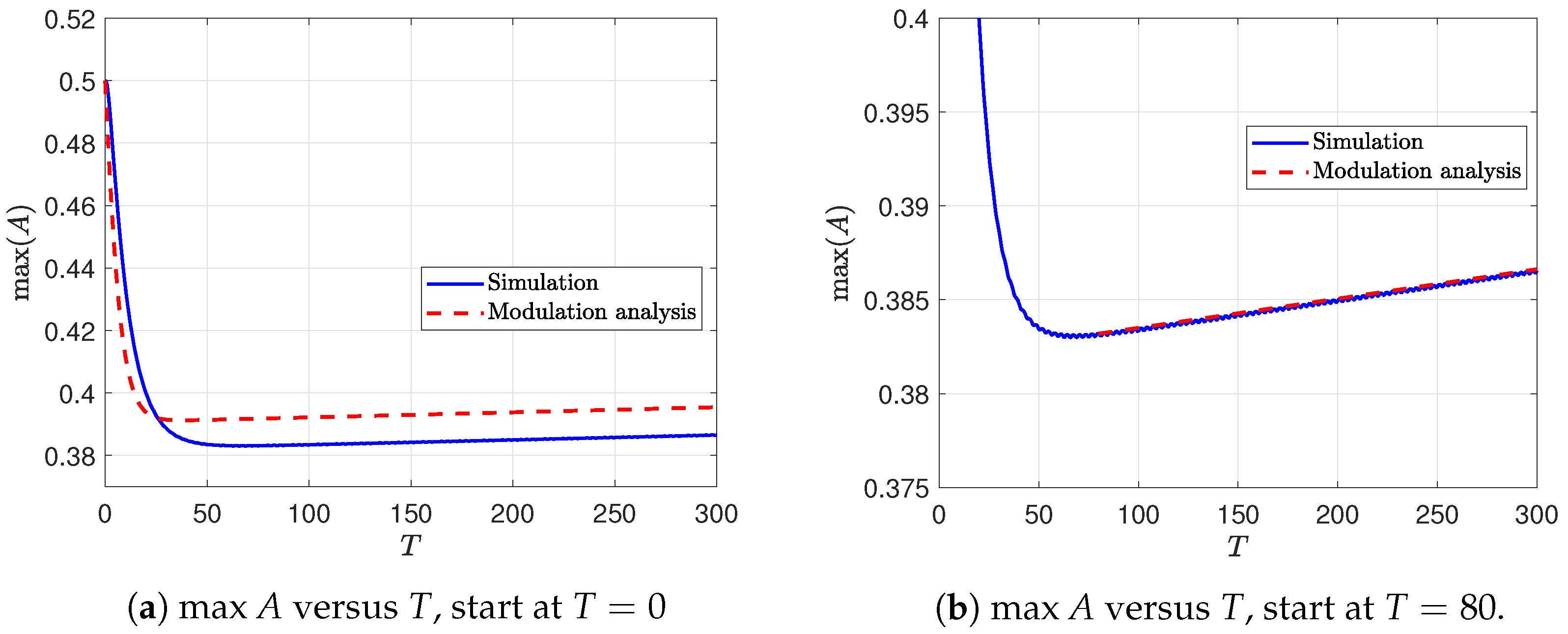
The initial solitary wave amplitude and the linear shear flow (27) satisfies the mass constraint, set as . First, we consider a case when the depth (60) increases; we set . The results are shown in Figure 1, Figure 2 and Figure 3. In Figure 1a,b, the solitary wave decreases in amplitude as increases and decreases, see Figure 2a. A slowly varying trailing shelf is generated from the initial solitary wave, consistent with the mass-balance condition (55); the solitary wave propagates with constant speed when the depth transition is complete, . In Figure 2b, we confirm the relation (54), where k is a proportional constant fitted from . Figure 3a shows a wind-forced case with . Overall, the modulation analysis (57) agrees well with the simulation, but slightly underestimates the rapid initial drop in amplitude caused by the variable depth , but agrees with the long-term trend. Figure 3b shows the simulation restarted at . The modulation analysis and simulation now agree very well, with wave growth due to the wind forcing as expected.
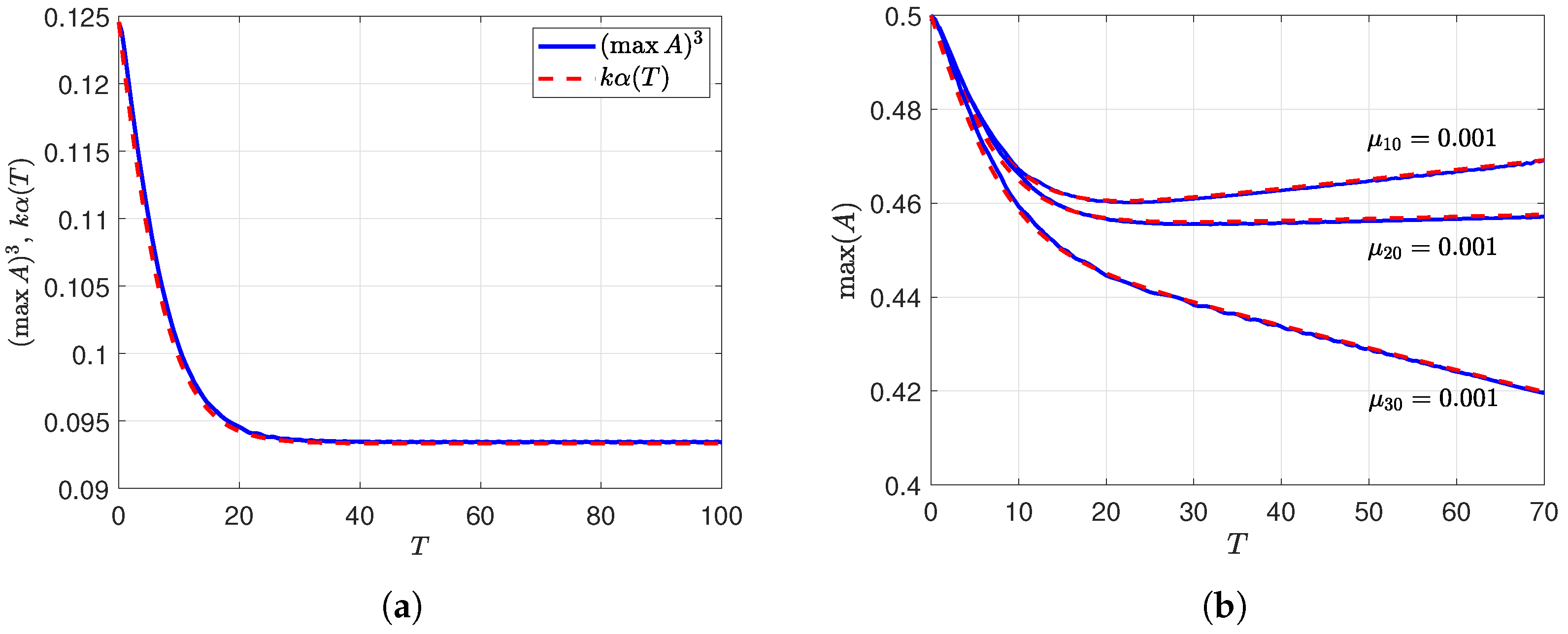
Figure 4 shows the same initial condition case for a weakly increasing depth . Now the solitary wave is essentially unchanged. Panel (a) shows that is very close to the modulation theory result . Panel (b) compares the simulation with modulation theory for all three forcing types; in each case, the agreement is very good. The bottom boundary layer term produces significant wave amplitude decay, as expected.
Figure 1.
Case A:
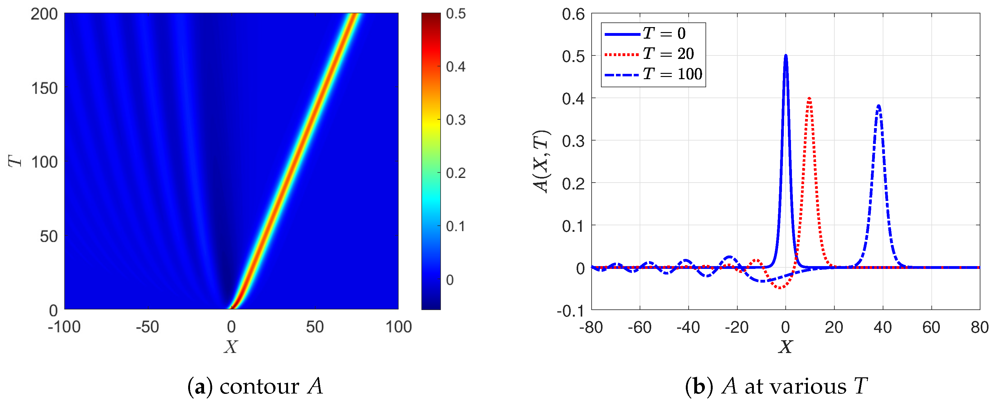
Figure 2.
Case A: .
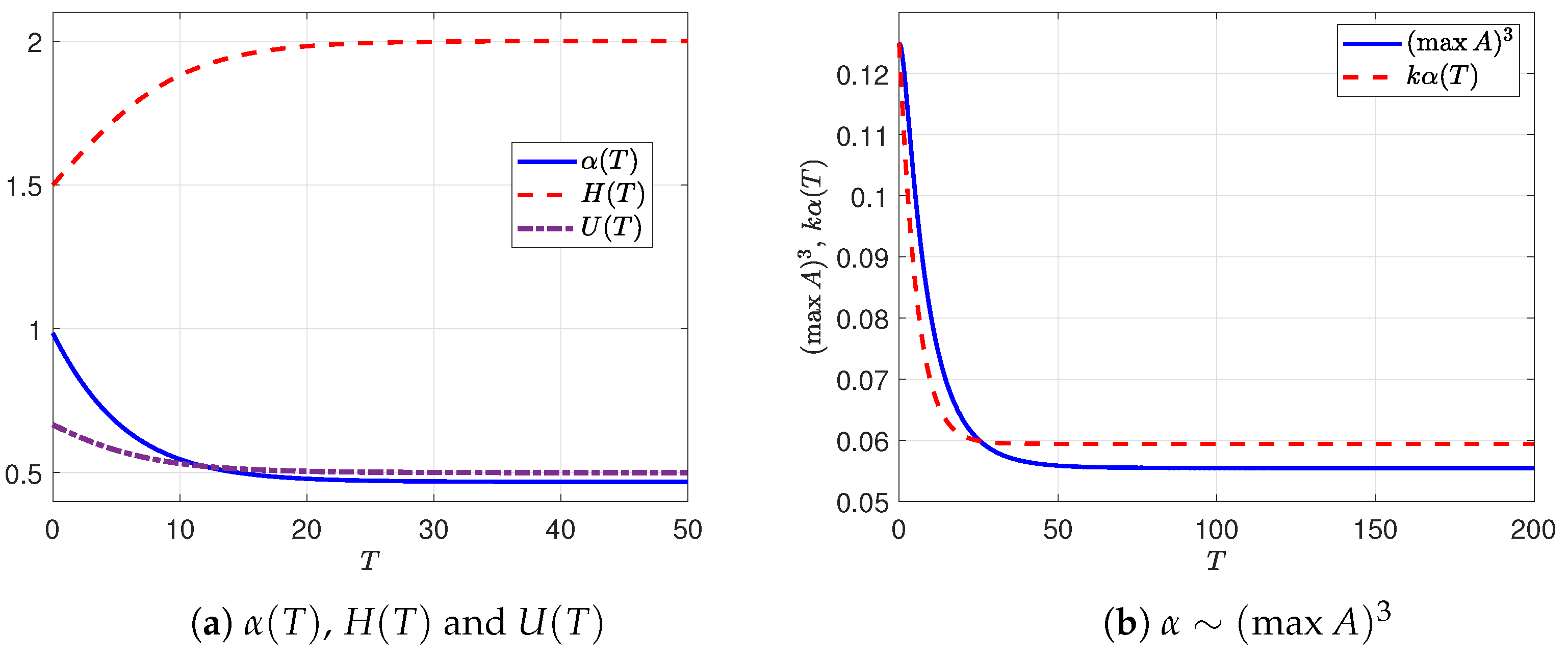
Figure 3.
Case A: , modulation analysis from Equation (57).
4.1.2. A: Decreasing Depth
We choose the same initial condition and basic current as in Section 4.1.1, but now set . The results are shown in Figure 5 and Figure 6. In Figure 5a,b, the solitary wave now increases in amplitude as decreases and increases, see Figure 6a. A small trailing shelf develops behind the initial solitary wave, consistent with the mass-balance condition (55). Figure 6a shows that is again confirmed. In Figure 6b, we show the solitary wave amplitude evolution and wind forcing effect with . The simulation with shows the purely adiabatic deformation due to the changing depth. When there is a small wind forcing term with , the wave amplitude grows as expected and agrees well with modulation analysis (57).
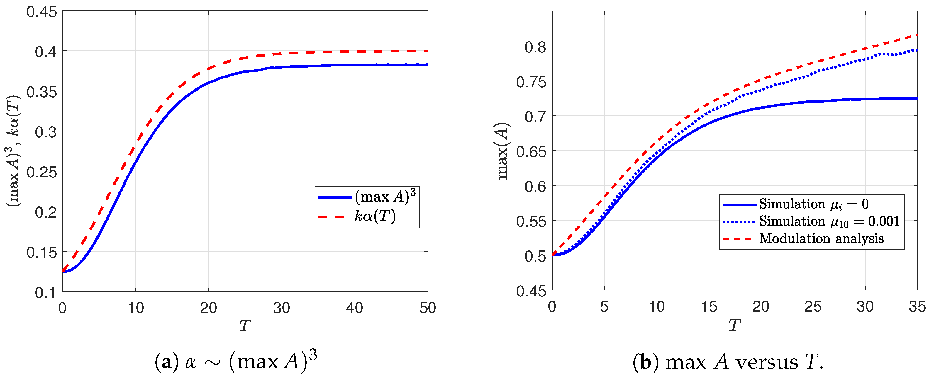
Figure 7 shows the same initial condition case for a weakly decreasing depth. . Panel (a) shows that is very close to the modulation theory prediction . Panel (b) compares the simulation with modulation theory for all three forcing types, with good agreement in each case. For the same forcing magnitudes , the critical level instability in the air now produces a stronger effect of wave growth than the wave stress from the air as the solitary wave moves into shallower water, consistent with the expressions (61).
Figure 5.
Case A: .
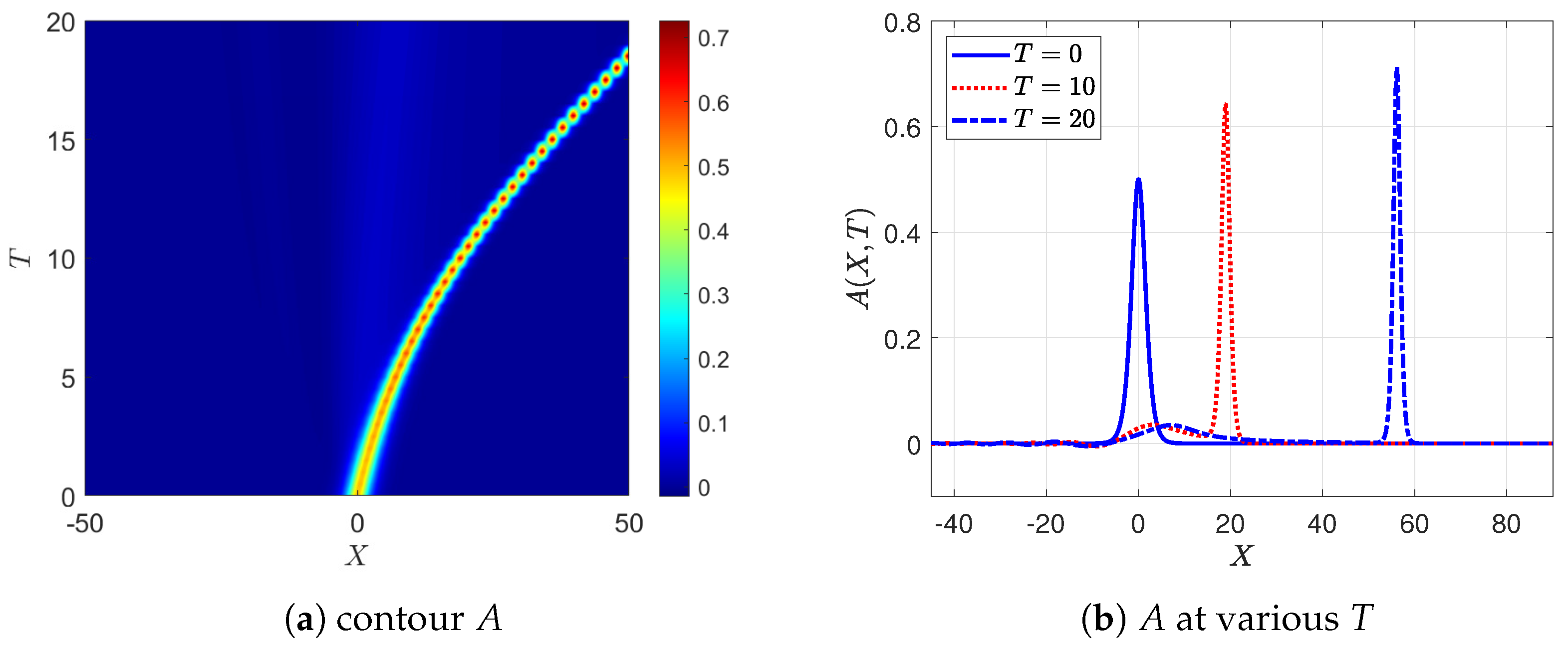
Figure 6.
Case A: (a) (b) .
4.2. Case B
4.2.1. B: Increasing Depth
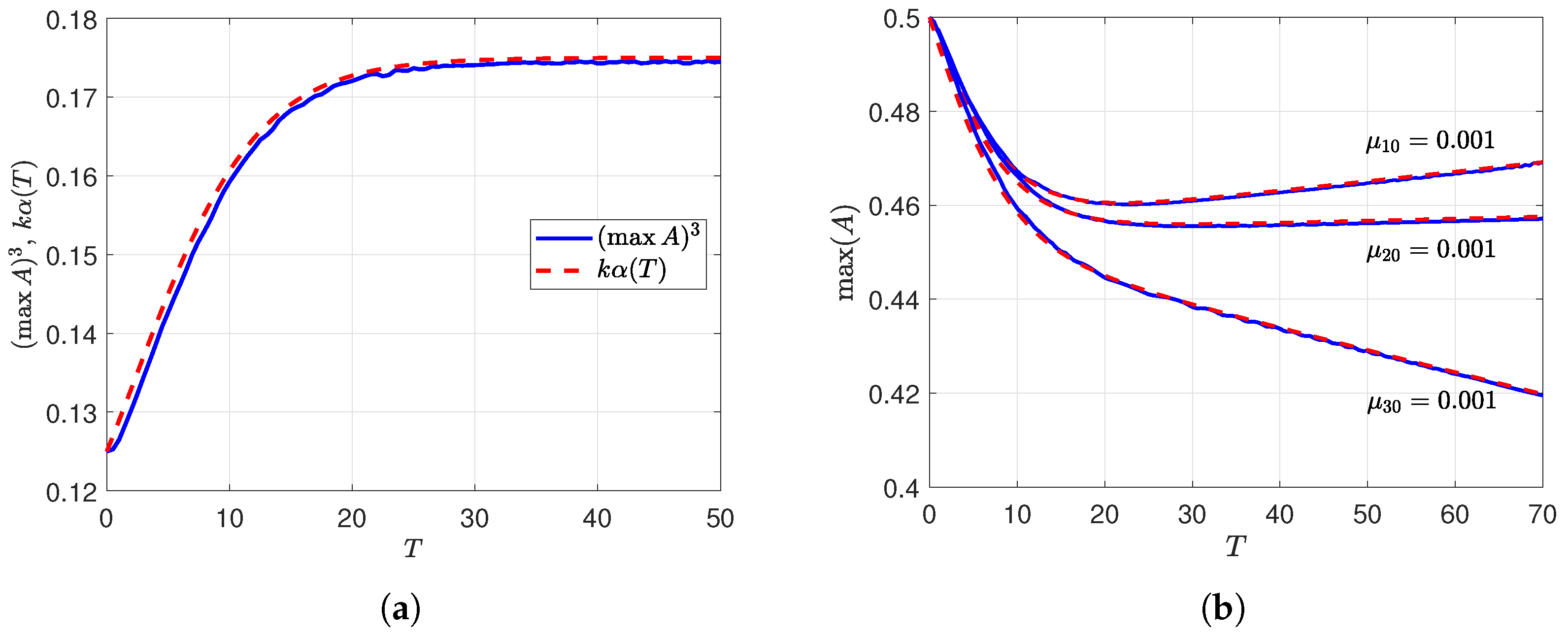
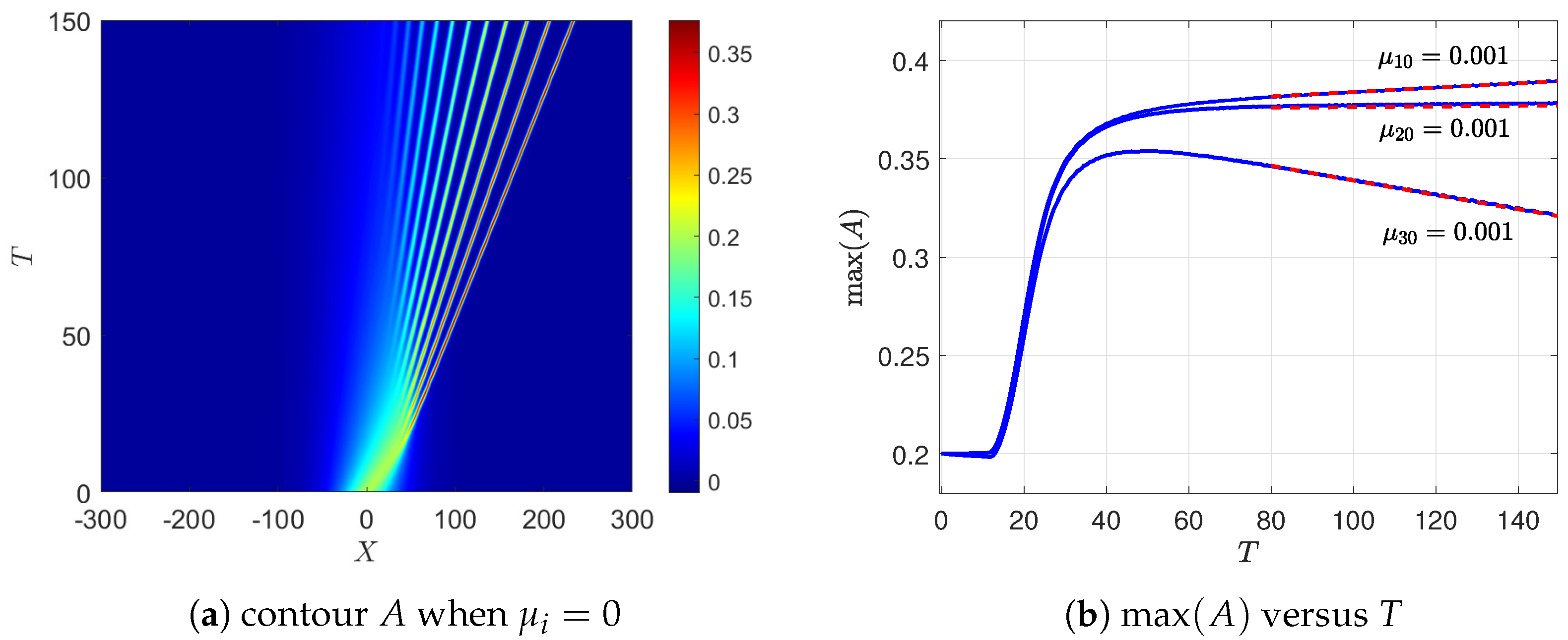
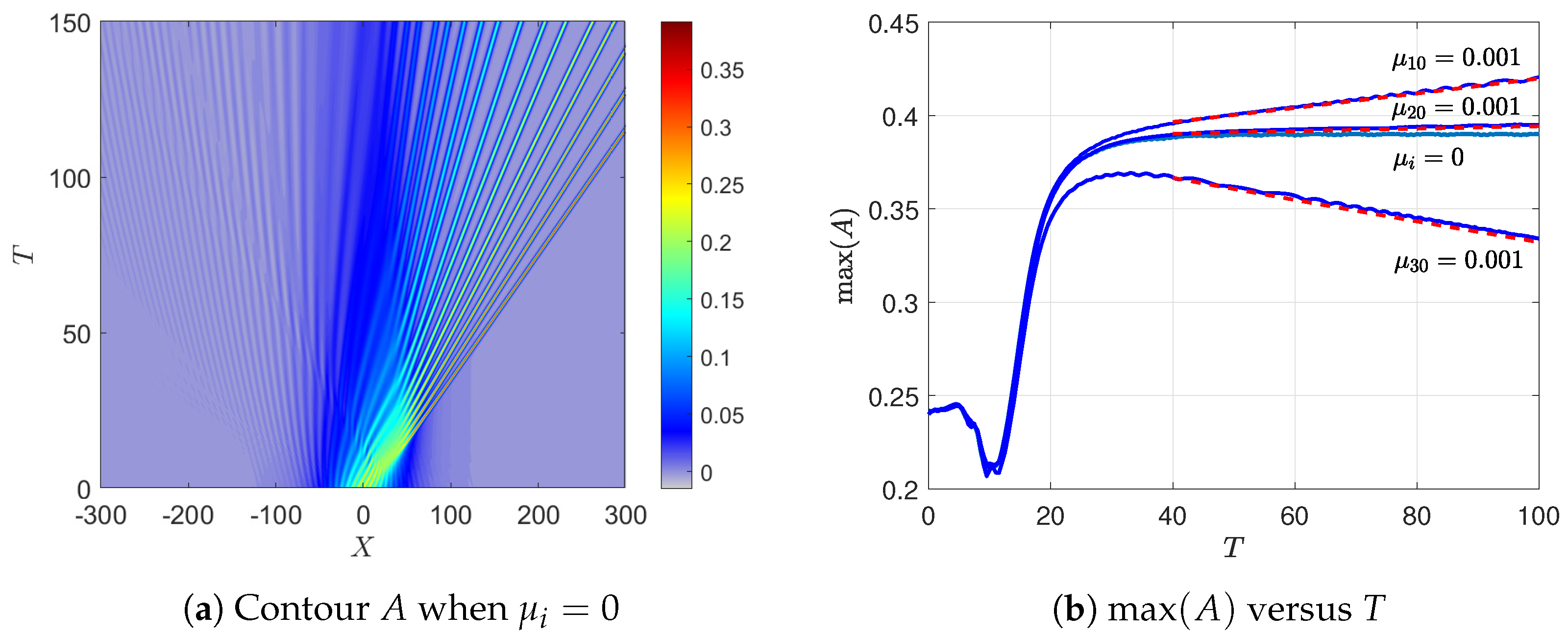
For Case B with an increasing depth, we set for the background flow, and for the initial condition. Figure 8a for an unforced case, , shows solitary waves initially exhibiting a short initial stage, when the linear dispersive term is very small, and the solution obeys a Hopf equation, preserving the maximum amplitude, with steepening on the front face, and formation of an expansion fan on the rear face; a stable solitary wave train then forms, adjusting to the deeper depth transition, and then reaching a steady maximum amplitude of at , consistent with the modulation theory (52). When the forcing terms are separately introduced in Figure 8b, the wind growth term produces an increase in the maximum amplitude, the nonlinear wave stress term produces a slower growth, and the bottom stress term leads to decay. After starting the comparison at , the modulation analysis (57)–(59) agree very well with the simulation for all three forcing cases.
4.2.2. B: Decreasing Depth
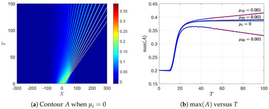
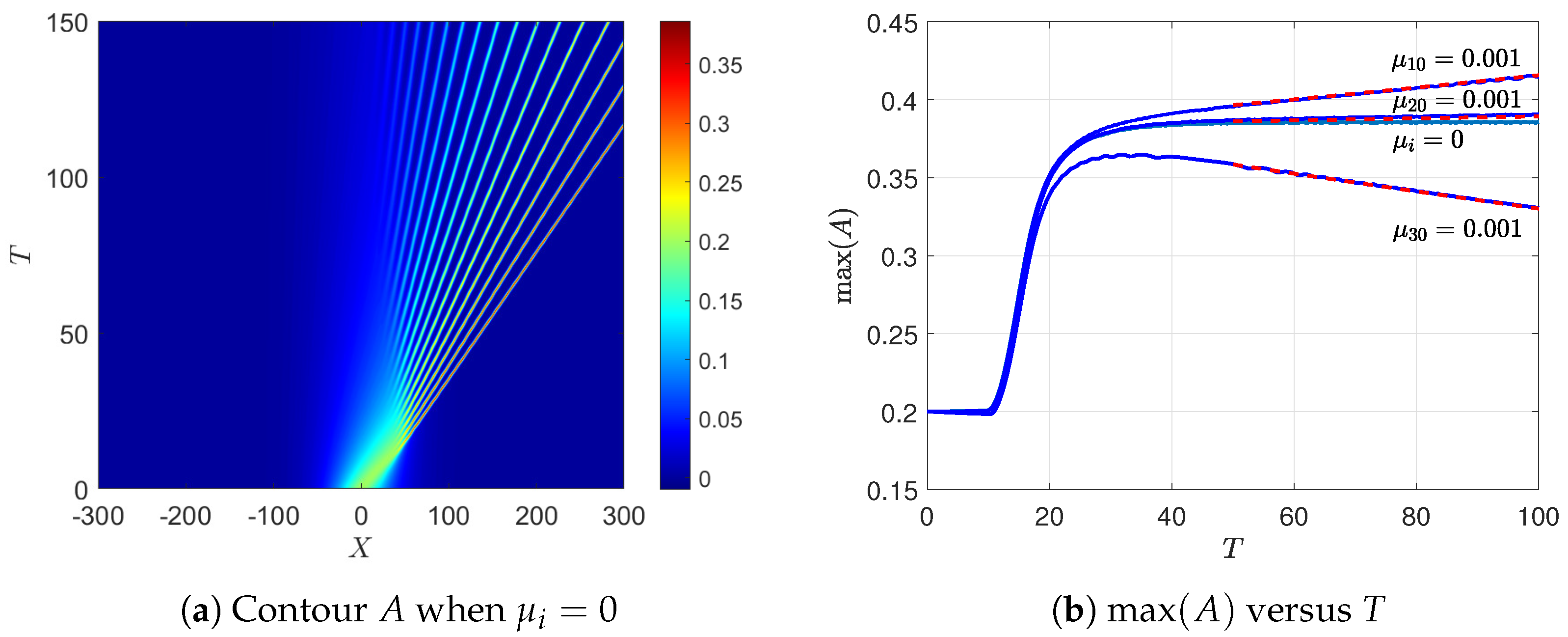
For Case B with a decreasing depth, we set , and again set for the initial condition. Figure 9a shows that in the unforced case (), the behaviour is similar to that for the case in Section 4.2.1 shown in Figure 8a, the final steady maximum amplitude is at when the depth is constant. In Figure 9b, the effects of the individual forcing terms are again consistent with the modulation theory; produces a slow increase in the maximum amplitude, shows a long-term growth, leads to wave decay. After starting the comparison at , the modulation analysis (57)–(59) agrees very well with the simulation for all forcing cases.
4.3. Case C
4.3.1. C: Decreasing Depth
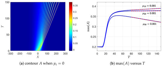
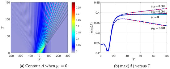
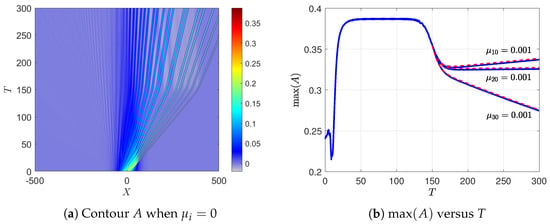
The initial condition is with . Figure 10a shows that in the unforced situation (), the perturbed envelope adjusts rapidly to the decreasing depth and background flow with . The initial envelope wave is periodically perturbed with a magnitude ; the solitary wave train settles after the initial transient and remains stable under this small initial perturbation. Figure 10b compares the maximum amplitude with the modulation theory; with the comparison starting at , the modulation analysis agrees very well with the simulation for all forcing cases.
4.3.2. C: Increasing Depth
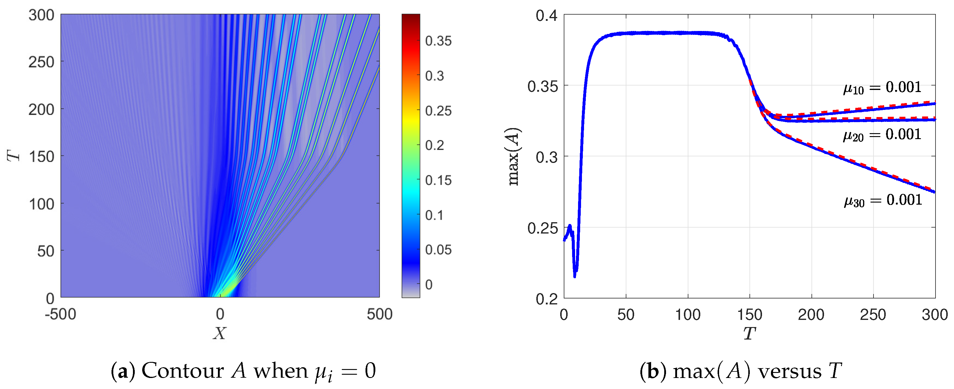
The initial condition is the same as in Section 4.3.1, with a small periodic perturbation, but here the water depth variation is delayed with so that a fully developed solitary wave train forms before encountering the depth transition. The background flow satisfies . For the unforced case, , Figure 11a shows the solitary wave train propagating over constant depth , stable over , with small oscillations in the maximum amplitude due to the perturbation. When the depth transition begins for approximately , the leading solitary wave accelerates and a trailing shelf becomes clearly visible. Figure 11b compares the maximum amplitude with the modulation theory starting at , when the solitary wave train is already well established. The agreement is very good for all three forcing mechanisms, confirming that once the solitary wave train reaches its asymptotic form, the modulation theory captures the effects of the depth transition and all three types of forcing.
5. Discussion and Summary
In this paper, we have extended our work in MG24 on the KdV–Burgers (KdVB) equation for the generation of wind waves in shallow water to allow for a slowly varying depth, and a background current. The outcome is a variable-coefficient KdVB Equation (8) where the slowly varying depth and background current are incorporated into a single slowly-varying nonlinear coefficient , (10), where T is a time-like variable describing the travel time of a linear long wave. The main factors determining are the depth and the surface current which satisfies the mass constraint ; together, these determine the linear long wave speed ; see (27) for our main illustrative example of a linear shear profile for the background current. The description of the variable-coefficient KdVB equation and an outline of its derivation are in Section 1 and Section 2. In Section 3, we re-visit the well-known modulation theory for the KdV equation, with a focus on the solitary wave train limit in which the amplitude varies as subject to the effect of the wind forcing terms. Numerical simulations of (8) are presented in Section 4 using initial conditions similar to those in MG24. In Section 4.1, the initial condition is a solitary wave which, in the absence of background variation and wind forcing, would propagate steadily unchanged in form; the modulation theory prediction of growth as is confirmed, along with the modulation theory predictions of the wind-forcing terms. In Section 4.2, the initial condition is a long wave perturbation which in MG24 was found to produce a solitary wave train; here we find that also, subject to the predictions of the modulation theory. The stability of this solitary wave train was tested numerically in Section 4.3 with the addition of a small sinusoidal perturbation, and was found to be stable.
In MG24 we showed that the KdVB equation was a useful model for wind-generated waves in shallow water, with typical solutions exhibiting solitary wave trains, forming a soliton gas. Importantly, this was noted by Costa et al. [8] in an examination of ocean data in a shallow sea using just the KdV equation; more recently Zdyrski and Feddersen [24], Manna and Latifi [25] studied an unstable KdV–Burgers equation, numerically and analytically respectively. In this paper we have demonstrated that inclusion of variable depth and a background current does not change this conclusion, modulo the adiabatic amplitude variation of . A major disadvantage of the KdV–Burgers model is that is one-dimensional in the horizontal space domain. For weak two-dimensional dispersion, the KdV–Burgers equation was extended in Maleewong and Grimshaw [7] to a KP-Burgers equation; in Maleewong and Grimshaw [26] we made a further extension to a forced Benney–Luke equation, which preserves isotropy in the horizontal domain. The same extensions can be made here and will be the subject of future research.
Author Contributions
Conceptualization, R.G.; Methodology, R.G.; Software, M.M.; Validation, R.G. and M.M.; Formal analysis, R.G.; Investigation, R.G. and M.M.; Data curation, M.M.; Writing—original draft preparation, R.G. and M.M.; Writing—review and editing, R.G. and M.M.; Visualization, M.M. All authors have read and agreed to the published version of the manuscript.
Funding
This research received no external funding.
Institutional Review Board Statement
Not applicable.
Informed Consent Statement
Not applicable.
Data Availability Statement
The raw data supporting the conclusions of this article will be made available by the authors on request.
Conflicts of Interest
The authors declare no conflicts of interest.
Appendix A. Numerical Scheme
The variable-coefficient KdV Equation (8) is solved numerically using a Fourier spectral method. We modify the main equation by inserting a damping term to absorb radiating waves approaching the far-field periodic boundaries,
Here denotes a sponge layer (or numerical absorber) used to prevent spurious wave reflection at the computational boundaries. It is defined by
where sets the damping strength, controls the smoothness of the damping transition, and marks the start of the absorbing region.
We split the evolution into a dispersive linear part and a time-dependent nonlinear part ,
Let denote the Fourier transform of . Introducing an integrating factor
This solves exactly the linear dispersive term and yields the system
Each term in the nonlinear part is solved using the fast Fourier transform at a specific time. The sponge layer is handled in the physical space, then the nonlinear part is transformed into the Fourier space . We apply the fourth-order Runge–Kutta method to solve (A1). Finally, the unknown A is obtained by taking the inverse Fourier transform of . Most of our simulations are performed over the spatial domain with time step and Fourier modes. The sponge layer is implemented using , , and .
References
- Grimshaw, R. Evolution equations for long nonlinear internal waves in stratified shear flows. Stud. Appl. Math. 1981, 65, 159–188. [Google Scholar] [CrossRef] [Scilit]
- Grimshaw, R.; Liu, Z. Nonlinear periodic and solitary water waves on currents in shallow water. Stud. Appl. Math. 2016, 139, 60–72. [Google Scholar]
- Johnson, R.S. Some numerical solutions of a variable-coefficient Korteweg-de Vries equation (with applications to solitary wave development on a shelf). J. Fluid Mech. 1972, 54, 81–91. [Google Scholar]
- Johnson, R.S. On the development of a solitary wave moving over an uneven bottom. Proc. Camb. Phil. Soc. 1973, 73, 183–203. [Google Scholar] [CrossRef] [Scilit]
- Craig, W.; Guyenne, P.; Sulem, C. Water waves over a random bottom. J. Fluid Mech. 2009, 640, 79–107. [Google Scholar] [CrossRef] [Scilit]
- Maleewong, M.; Grimshaw, R. Evolution of water wave packets by wind in shallow water. J. Fluid Mech. 2024, 996, A4. [Google Scholar] [CrossRef] [Scilit]
- Maleewong, M.; Grimshaw, R. Evolution of wind-generated shallow water waves in the framework of a modified Kadomtsev-Petviashvili equation. Fluids 2025, 10, 61. [Google Scholar]
- Costa, A.; Osborne, A.R.; Resio, D.T.; Alessio, S.; Chrivì, E.; Saggese, E.; Bellomo, K.; Long, C.E. Soliton turbulence in shallow water ocean surface waves. Phys. Rev. Lett. 2014, 113, 108501. [Google Scholar] [CrossRef] [Scilit] [PubMed]
- El, G.A. Soliton gas in integrable dispersive hydrodynamics. J. Stat. Mech. 2021, 2021, 114001. [Google Scholar] [CrossRef] [Scilit]
- Zhou, X.; Grimshaw, R. The effect of variable currents on internal solitary waves. Dyn. Atmos. Oceans 1989, 14, 17–39. [Google Scholar] [CrossRef] [Scilit]
- Miles, J.W. On the generation of surface waves by shear flows. J. Fluid Mech. 1957, 3, 185–204. [Google Scholar] [CrossRef] [Scilit]
- Freeman, N.; Johnson, R.S. Shallow water waves on shear flows. J. Fluid Mech. 1970, 42, 401–409. [Google Scholar] [CrossRef] [Scilit]
- Liu, Z.; Grimshaw, R.; Johnson, E. Internal solitary waves propagating through variable background hydrology and currents. Ocean Model. 2017, 116, 134–145. [Google Scholar] [CrossRef] [Scilit]
- Liu, Z.; Grimshaw, R.; Johnson, E. The effect of variable background hydrology and currents on oceanic internal solitary waves. Fluids 2018, 3, 96–119. [Google Scholar]
- Burns, J.C. Long waves in running water. Proc. Camb. Phil. Soc. 1953, 49, 695–706. [Google Scholar] [CrossRef] [Scilit]
- Kharif, C.; Abid, M. Nonlinear water waves in shallow water in the presence of constant vorticity: A Whitham approach. Eur. J. Mech. B Fluids 2018, 72, 12–22. [Google Scholar] [CrossRef] [Scilit]
- Whitham, G.B. Linear and Nonlinear Waves; Wiley: Hoboken, NJ, USA, 1974. [Google Scholar]
- Grimshaw, R.; Yuan, C. Internal undular bores in the coastal ocean. In The Ocean in Motion; Velarde, M., Tarakanov, R., Marchenko, A., Eds.; Springer Oceanography Series; Springer: Berlin/Heidelberg, Germany, 2018; Volume 7, pp. 23–39. [Google Scholar]
- Grimshaw, R.; Yuan, C. The propagation of internal undular bores over variable topography. Phys. D 2016, 333, 200–207. [Google Scholar] [CrossRef] [Scilit]
- El, G.A.; Grimshaw, R.H.J.; Tiong, W.K. Transformation of a shoaling undular bore. J. Fluid Mech. 2012, 709, 371–395. [Google Scholar] [CrossRef] [Scilit]
- Grimshaw, R. The solitary wave in water of variable depth. J. Fluid Mech. 1970, 42, 639–656. [Google Scholar] [CrossRef] [Scilit]
- Grimshaw, R.H.J.; Pudjaprasetya, S.R. Generation of secondary solitary waves in the variable-coefficient Korteweg–de Vries equation. Stud. Appl. Math. 2004, 112, 271–279. [Google Scholar]
- Grimshaw, R. Slowly varying solitary waves i. Korteweg-de Vries equation. Proc. R. Soc. 1979, 368A, 359–375. [Google Scholar] [CrossRef] [Scilit]
- Zdyrski, T.; Feddersen, F. Wind-induced changes to surface gravity wave shape in shallow water. J. Fluid Mech. 2021, 903, A27. [Google Scholar]
- Manna, M.A.; Latifi, A. Korteweg de Vries—Burger equation with Jeffreys wind wave interaction: Blow-up and breaking of soliton-like solutions in finite time. Fluids 2023, 8, 231–244. [Google Scholar]
- Maleewong, M.; Grimshaw, R. Evolution of wind-generated shallow water waves in a Benney–Luke equation. Ocean Model. 2026, 200, 102659. [Google Scholar]
Disclaimer/Publisher’s Note: The statements, opinions and data contained in all publications are solely those of the individual author(s) and contributor(s) and not of MDPI and/or the editor(s). MDPI and/or the editor(s) disclaim responsibility for any injury to people or property resulting from any ideas, methods, instructions or products referred to in the content. |
© 2026 by the authors. Licensee MDPI, Basel, Switzerland. This article is an open access article distributed under the terms and conditions of the Creative Commons Attribution (CC BY) license.