Autoencoder-Based Optimal Sensor Placement and Aerodynamic Load Reconstruction for Airfoils

Abstract

Optimal sensor placement is a crucial issue in scientific and engineering research. This study proposes an autoencoder-based deep learning framework for automated optimal sensor layout and flow field reconstruction. A dataset is established based on transient Computational Fluid Dynamics (CFD) simulation results of a three-dimensional finite-span airfoil under various Reynolds numbers and angles of attack, enabling high-precision reconstruction of airfoil surface pressure distribution using sparse pressure coefficient data. The multilayer perceptron of both the encoder and decoder adopts an optimal five-layer structure with 200 nodes per layer, and the ReLU activation function delivers superior performance with a training loss reduction of over 45%. When using 50 sensors, the proposed architecture determined detailed placement and obtained a reconstruction error of 0.0604, which outperforms traditional manual sensor placement. The reconstruction accuracy of aerodynamic loads improves with increasing sensor count, but exhibits diminishing returns beyond the optimal threshold 50, necessitating a balanced selection that optimizes performance-to-cost ratio. The proposed method adaptively captures critical flow regions with high gradients, cutting sensor quantity by 60–80% versus grid-based placement. This method can flexibly use either CFD or experimental data in practical applications, offering an efficient solution for aerodynamic field reconstruction.

1. Introduction

As one of the key indexes to evaluate the aerodynamic performance of airfoil, the aerodynamic load distribution plays an important role in engineering applications such as wing shape optimization [1], flow separation control [2], and flight control [3]. Local aerodynamic load data can be obtained by deploying sensors at specific positions; however, the number of sensors and spatial placement strategy directly affect the measurement accuracy. Overly dense configurations may perturb the local flow field, introduce systematic errors, and escalate system complexity, whereas sparse layouts fail to capture spatial gradients essential for full-field estimation. In fact, optimizing the arrangement of a limited number of sensors to achieve high-precision state estimation or fluid flow control is a scientific and engineering problem with a wide range of practical applications, which often appears in hydraulic machinery [4], nuclear reactor [5], construction engineering [6,7], water supply network [8], structural system identification and damage detection [9,10], aircraft aerodynamic structure control [11], etc. In airfoil-specific contexts, research priorities include airfoil wake estimation [12], flow field reconstruction [13], optimal vector sensor layout [14], real-time flow observation [15] and others.

The research direction of intelligently determining sensor placements with the goal of saving instrument costs and improving the prediction accuracy of target physical quantities is one of the hotspots at present. Existing methods include optimization method, reduced order modeling, machine learning, etc. The optimization methods mainly consist of the nonlinear programming method, simulated annealing algorithm, genetic algorithm and particle swarm optimization algorithm. For example, Nasr et al. [16] used the genetic algorithm to determine the optimal position of sensors in the process of structural system damage detection through the minimization process of cost function, and achieved good prediction accuracy. However, the optimization method has some disadvantages, such as the amount of calculation of evolutionary algorithms increases with the increase in algebra, and the calculation of gradient matrix of nonlinear programming method is very complex. When extended to the field of flow and heat transfer, the degree of freedom is usually more than one million, so the optimization method faces the challenges of complexity and computational cost. Reduced order modeling including the Proper Orthogonal Decomposition (POD), the Dynamic Mode Decomposition (DMD) and other methods have also been used to infer the optimal position of the sensor in flow and heat transfer problems. For example, Cohen et al. [17] determined the sensor placement by placing the sensor at the extreme value of POD mode; Kumar et al. [18] inferred the sensor position on the two-dimensional airfoil by minimizing the error between the linear stochastic estimation (LSE) prediction and POD modal amplitude. However, due to the limited sensitivity of LSE to sensor positions, this method has great uncertainty. Although the accuracy can be improved by the increase in the number of modalities and snapshots involved, the decomposition process requires a huge amount of calculation. On the other hand. Sashittal et al. [19] introduced a DMD-based data-driven sensor placement method for fluid flows, using adjoint optimization to minimize estimation error covariance trace via linear dynamic approximation, validated via flat plate flow applications. Barklage et al. [20] proposed a Bayesian extension to the Gappy POD data fusion method, and incorporated an efficient genetic algorithm for sensor placement to achieve optimal aerodynamic data fusion for two-dimensional airfoils and three-dimensional NASA general research models.

With the rise in artificial intelligence (AI) technology [21,22,23], machine learning (ML) and deep learning (DL) are gradually used to carry out the research of optimal sensor placement. For example, R. Semaan [24] used Random Forest algorithm to predict the relationship between the pressure/shear stress at the measuring points on the surface of the airfoil with the Konda flap and the flow field performance, and then used the out-of-bag samples to determine the importance of input variables, so as to select the optimal sensors. Although this is a relatively successful attempt of machine learning in this kind of problem, Random Forest is easy to over fit, especially in regression problems, which limits the generalization ability. Kelmar et al. [25] used similar methods to predict the natural frequency of the wing, providing a new perspective for improving the efficiency and accuracy of modal test procedures in aircraft structural design. Deng et al. [26] studied the optimal sensor placement strategy for turbulence recovery based on deep neural network under the framework of Ensemble Kalman Filter data assimilation. They designed the feature importance layer and took the corresponding position with the largest weight value in this layer as the optimal position of the experimental sensor. However, this method is lack of strict proof in mathematics since there are a large number of weight parameters from this layer to the output layer, and the weight between the input layer and the feature importance layer cannot strictly guarantee the importance of the input feature. Furthermore, there have been studies on optimal sensor placement for active flow control around a cylinder using reinforcement learning [27] recently.

The current research on optimal sensor placement in fluid flow mainly focuses on the problem of flow around a cylinder [28], and some research is extended to airfoil sensors/actuators. However, the existing research is mostly based on the simplified two-dimensional airfoils [1,2,3], which has significant differences between the model and the engineering issues. On the other hand, with the rapid development of AI technology, the research on optimal placement of three-dimensional airfoil sensors based on deep learning has become technically feasible, which promotes the transformation of sensor layout research from two-dimensional simplification to three-dimensional refinement, so as to improve the consistency between the theoretical model and engineering practice, and provide more reliable technical support for practical application. As a representative scientific machine learning framework developed based on PyTorch (e.g., PyTorch 2.10.0), NVIDIA’s open-source PhysicsNeMo [29] integrates embedded physics-AI modules and enables AI model training driven by both data and first principles. Recently, it has been adopted to achieve rapid screening of sites for carbon capture and storage [30]. Additionally, the Workshop on Machine Learning for Fluid Mechanics [31] has continuously advanced research frontiers covering data-driven turbulence modeling, reduced-order modeling, flow field super-resolution reconstruction, uncertainty quantification and machine learning accelerated solvers. Collectively, these progresses establish a solid technical foundation for the data-driven sensor placement and flow field reconstruction framework proposed in the present work.

This study makes a rational trade-off in the selection of deep learning frameworks. Targeting the optimization of sensor placement for airfoils with surface pressure distribution as the typical aerodynamic load, an autoencoder-based deep learning framework is accordingly proposed. In this paper, the airfoil pressure distribution is taken as the typical aerodynamic load analysis object, and a deep learning framework based on autoencoder is proposed. With the candidate sensors and the number of sensors to be selected given, the sensors placement is automatically determined, and the three-dimensional flow field of airfoil is reconstructed from the sensor monitoring data. The sensor data is simulated by extracting the data at a specific location from Computational Fluid Dynamics (CFDs) simulation results. Therefore, the remaining of this paper is arranged as follows: Section 2 introduces the establishment of the CFD simulation database of the flow field, including the verification of CFD numerical algorithm, the establishment process of the database and the layout of the candidate sensors; Section 3 focuses on the sensor placement strategy framework based on deep learning; Section 4 shows and discusses the results of the optimal sensor placement strategy proposed in this study and reconstruction accuracy, with analysis of the training of the overall model including encoder and decoder and the training of the encoder model only, as well as the discussion on influencing factors and advantages and limitations of the study; finally, the conclusions and prospects of this paper are drawn in Section 5.

2. Database Establishment of Transient Airfoil Flow Field and Training Data Generation

In this study, the finite-span three-dimensional unsteady Reynolds-averaged Navier–Stokes (URANS) turbulence modeling of the classic airfoil NACA 4412 is carried out. The case studies cover flows ranging from complete flow separation to almost complete flow attachment. This section first introduces the details of the selected airfoil, followed by descriptions of the numerical algorithm, grid, governing equations, and turbulence model. Finally, the simulation results and their verification are presented.

2.1. Verification of CFD Algorithm

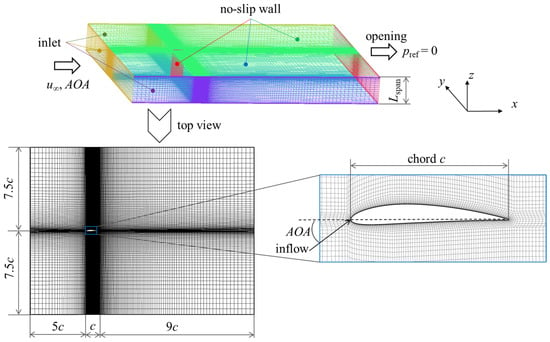
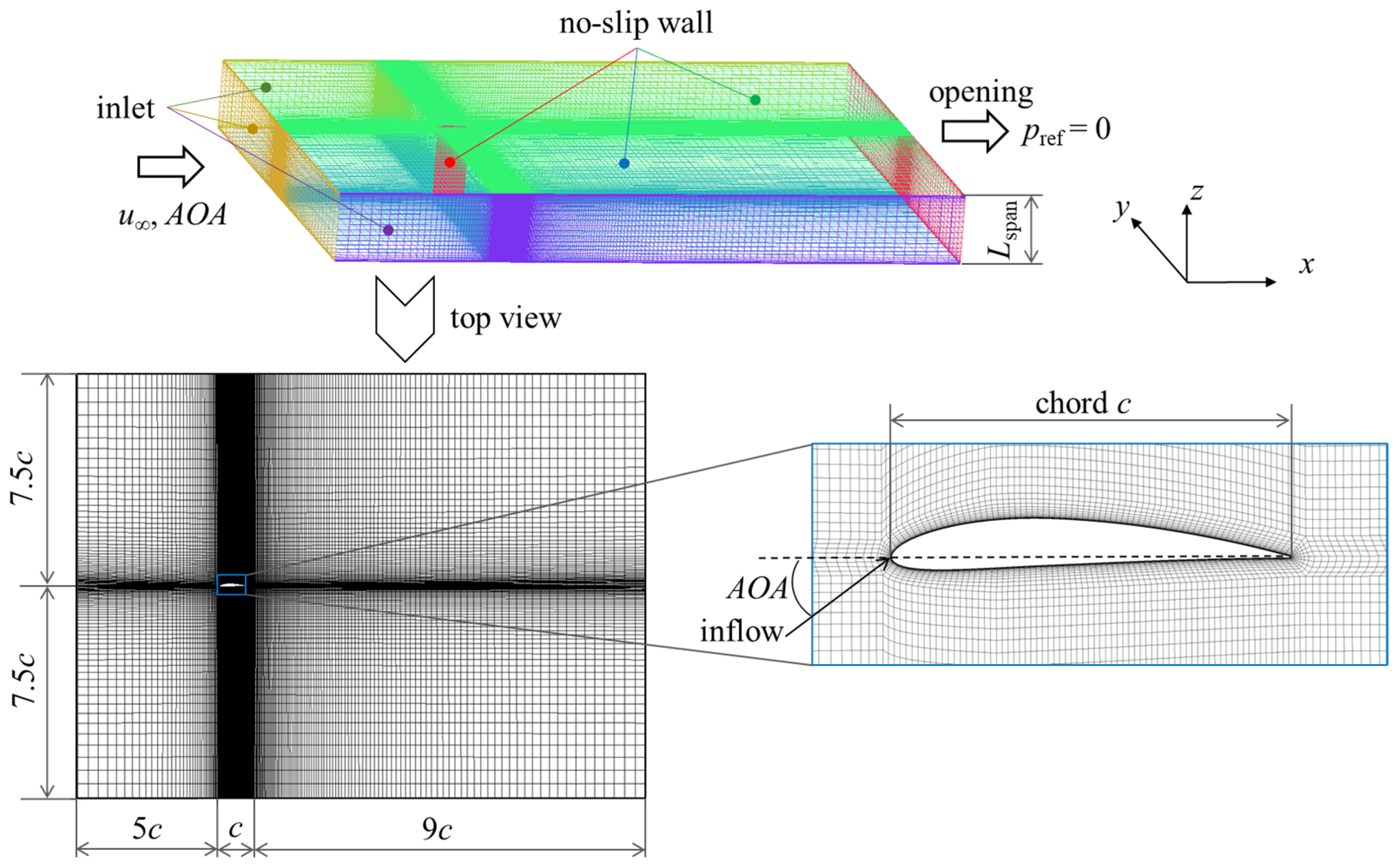
NACA 4412 is an asymmetric airfoil, and its main geometric parameters and experimental operating conditions [32] for numerical algorithm verification are shown in Table 1. Figure 1 shows the schematic diagram of the computational domain and grid. The entrance of the computational domain is 5 c away from the leading edge, the outlet is 9 c away from the trailing edge, and the side is 7.5 c respectively, where c donates for the chord. The height of the computation domain is L_span, i.e., the airfoil span. The boundary conditions are set as follows: the inlet boundary condition is given the value and direction of the incoming flow velocity u_∞, where the subscript “∞” indicates the value of incoming flow; the flowing medium is the air with the density ρ = 1.185 kg/m³, and the dynamic viscosity μ = 1.831 × 10⁻⁵ Pa·s; the downstream is an opening outlet, with the reference pressure p_ref set as 0; the airfoil surface and spanwise walls are non-slip walls.

Table 1. Main geometric and experimental operating condition parameters of the NACA 4412 airfoil.

Quantity	Units	Value
Chord (c)	mm	901.2
Airfoil span (Lspan)	mm	1991
Angle of attack (AOA)	°	14
incoming velocity (u∞)	m/s	26.06
Reynolds number (Re)	/	1.52 × 106

Figure 1. Schematic diagram of computational domain, boundary conditions and grid.

Given that the maximum Mach number under the operating conditions investigated in this study is 0.077, three-dimensional incompressible numerical simulations were performed. The governing equations consist of the continuity equation and the momentum equation, which are expressed as follows:

$$\nabla ·\mathit{u}=0,$$

(1)

$${\displaystyle \frac{d\mathit{u}}{dt}}=-{\displaystyle \frac{1}{\rho }}\nabla p+{\displaystyle \frac{\mu }{\rho }}{\nabla }^2\mathit{u},$$

(2)

where u is the velocity, t represents the time and p is the pressure. The RNG k-ε model which is suitable for flow separations is adopted as the turbulence model [33]. The medium turbulence intensity (5%) is set for the inlet turbulence boundary condition, which is applicable to a wide range of engineering scenarios [34,35]. The ANSYS CFX 19.0 is selected as the CFD solver, in which a fully coupled solver is adopted and the pressure–velocity coupling is inherent during the solution procedures. The airfoil surface and spanwise walls are set as no-slip smooth walls with Scalable Wall Functions used. The convective term is discretized using the High-Resolution Scheme implemented in ANSYS CFX. In this scheme, the weighting coefficients used to evaluate the advective fluxes of transport variables at cell interfaces are determined according to the literature [36,37]. A Multigrid accelerated Incomplete Lower Upper factorization technique is employed for solving the discrete system of linearized equations. The residual criterion is set to 1 × 10⁻⁵.

Four groups of structured meshes with varying cell resolutions are generated for grid independence verification, and their respective cell counts are summarized in Table 2. Refined meshes are applied near the airfoil surface and spanwise walls, with the first-layer heights set to 0.02 and 0.1, respectively, yielding corresponding y⁺ values of 1.996 and 5.636. The mesh quality is quantified via the Quality index cited in Ref. [38], a standard criterion for mesh characterization. This composite index is defined as a weighted combination of three parameters: Determinant, maximum orthogonal quality (Max Orthogls), and maximum warpage (Max Warpgls). The Determinant is defined as the ratio of the minimum to maximum Jacobian determinant evaluated at all element nodes. Max Orthogls quantifies the largest angular deviation of element interior angles from 90°. For Max Warpgls, the warping of a quadrilateral face is obtained by computing the angular difference between two triangles split along the face diagonals and taking the resulting maximum value; the warpage of a hexahedral element is further defined as the peak warpage across all its quadrilateral faces. A Quality value approaching unity denotes superior mesh quality. For the four mesh configurations examined herein, the Quality distributions remain comparable, with the global minimum reaching approximately 0.503, and over 92% of mesh elements yielding Quality above 0.95. These statistics verify that all generated meshes possess satisfactory quality and satisfy the mesh specification criteria required for subsequent CFD computations.

Table 2. Comparisons between computational results under different mesh configurations and experimental data.

Mesh Name	Elements Number		CL
		Simulated Result	Experimental Result	Relative Error/%
Mesh 1	2.73 × 105	1.011	1.673 [32]	−39.56
Mesh 2	5.28 × 105	1.350		−19.29
Mesh 3	1.02 × 106	1.585		−5.25
Mesh 4	1.99 × 106	1.668		−0.27

Table 2 also shows the comparison between the simulated and experimental result of the lift coefficient C_L, where $C_L={\displaystyle \frac{F_L}{\frac{1}{2}\rho u_{\infty }^{2}c{L}_{span}}}$ and F_L represents the lift force. It is evident that as the grid is gradually densified, the relative errors between the simulated and experimental results of C_L tend to diminish. The error decreases to −5.25% and −0.27%, respectively, when the element number increase to about 1.02 million and 1.99 million, which verifies the numerical algorithm adopted in this study.

In addition, it should be noted that since sufficient training samples are required for the subsequent deep learning process, more than one hundred operating conditions and thousands of unsteady flow field are needed when establishing the database in the following sections. Therefore, Mesh 3 is selected for the following database establishment taking into account the calculation time, accuracy and data storage space constraints.

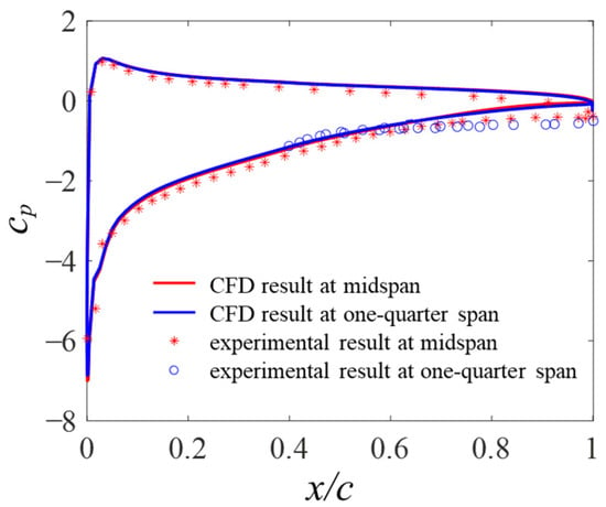
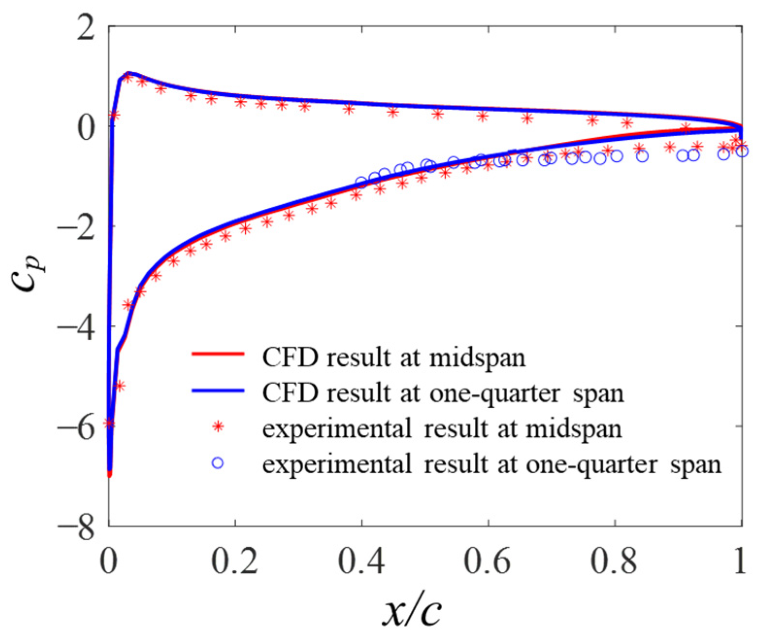
To conduct further verification, we take Mesh 3 as an example. Figure 2 presents the comparison of the pressure coefficient C_p between CFD results and the experimental data from Ref. [32] at the midspan and quarter span. Here, C_p is defined as follows:

$$C_p={\displaystyle \frac{p-p_{\infty }}{\frac{1}{2}{\rho }_{\infty }{u}_{\infty }^2}},$$

(3)

where p_∞ is the pressure of incoming flow. As shown in Figure 2, the simulated distribution of C_p over the airfoil surface agrees well with the experimental data. Specifically, minor discrepancies are observed over the forward two-thirds of the airfoil, and favorable consistency is also achieved in the leading-edge region with drastic pressure variations. Near the trailing edge, although the overall trend is well captured, certain deviations still exist. This phenomenon is likely attributed to the adoption of boundary-layer trips in the experiments [32], which are not incorporated in the present numerical simulations. Overall, the above validations demonstrate the reliability and efficacy of the proposed method, thereby verifying its applicability for subsequent dataset construction.

Figure 2. Comparisons of C_p between CFD result using Mesh 3 and experimental result [32] at midspan and one-quarter span.

2.2. Database Establishment of Transient Airfoil Flow Field

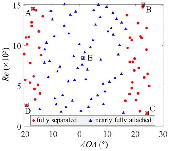
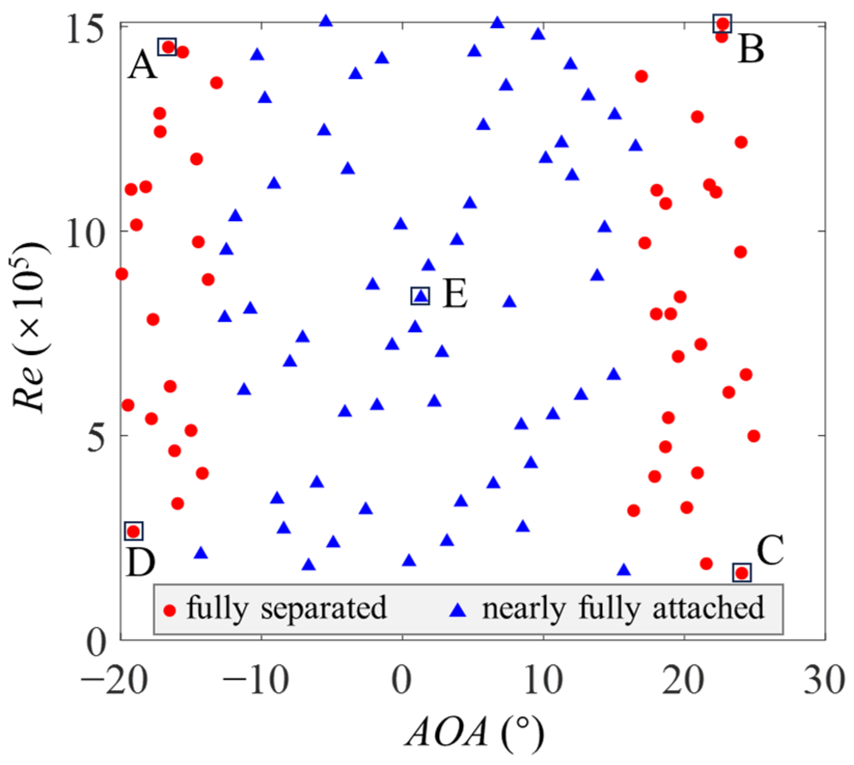
This section describes the establishment of the CFD transient database based on Mesh 3 described in Section 2.1. Numerical simulations under different Res and AOAs are carried out to obtain high spatial-temporal resolution flow field of airfoil. Specifically, the AOA range is from −20° to 25°, covering the operating conditions of large and small, positive and negative AOAs. The incoming velocity ranges from 2.606 to 26.06 m/s, with the corresponding Res varying from 1.52 × 10⁵ to 1.52 × 10⁶. Latin hypercube sampling (LHS) [39] was adopted to sample 108 operating conditions from the above AOA and Re range, as shown in Figure 3, which includes 48 large-scale flow separation conditions and 60 near fully attached/small-scale flow separation conditions.

Figure 3. Operating conditions of URANS simulation cases in the dataset. The letters represent 5 typical operating conditions.

We performed transient numerical simulations using the precomputed steady flow field as the initial field, with a time step of 0.002 s. The total simulation duration and field output interval (i.e., the number of snapshots) were determined based on the following considerations. This database is constructed to acquire flow fields under diverse operating conditions. A wider range of AOA and Re, richer flow regimes (large-scale separation, mild separation and nearly attached flow), and more diverse stages of unsteady flow evolution will produce datasets with higher sample diversity and more complex flow characteristics, which can better validate the DL method adopted in this work.

Therefore, for unsteady cases in this study, instantaneous flow fields are saved from the start of URANS simulation, rather than after the flow reaches a statistically stable state. In addition, the URANS simulations adopt steady flow fields precomputed by RANS as initial conditions, instead of meaningless zero-value fields. The obtained unsteady snapshots are more consistent with practical engineering scenarios, which include not only steady operating states but also transient flow variations induced by disturbances.

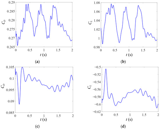
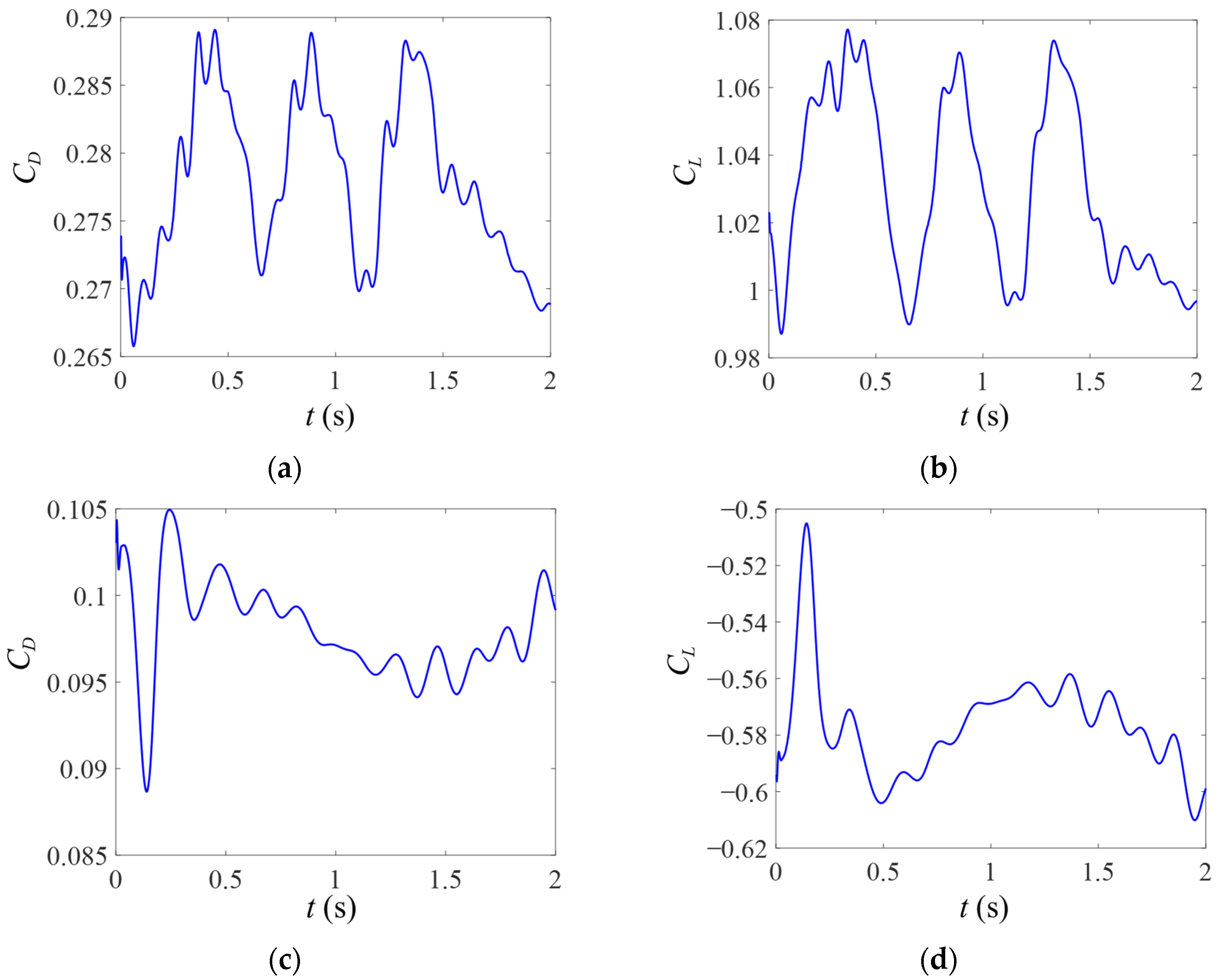
Figure 4 presents the time histories of C_D and C_L within 2 s for two typical cases with large scale flow separation, where $C_D={\displaystyle \frac{F_D}{\frac{1}{2}\rho u_{\infty }^{2}c{L}_{span}}}$ and F_D represents the drag force. Figure 4a,b correspond to a large positive AOA and high Re condition, featuring smaller characteristic time scales. Three to four vortex shedding cycles can be observed over the 2 s period. Figure 4c,d represent a large negative AOA and low Re condition, with larger characteristic time scales and drastic fluctuations in C_D and C_L. Accordingly, a total simulation duration of 2 s is sufficient to ensure adequate sample diversity.

Figure 4. Time histories of C_D and C_L under typical operating conditions in the test dataset. (a) C_D, Re = 1.22 × 10⁶, AOA = 24.02°; (b) C_L, Re = 1.22 × 10⁶, AOA = 24.02°; (c) C_D, Re = 3.34 × 10⁵, AOA = −15.96°; (d) C_L, Re = 3.34 × 10⁵, AOA = −15.96°.

The number of snapshots saved for each unsteady case was determined by balancing the sample requirements for subsequent training and validation, as well as disk storage constraints. Consequently, 51 snapshots were ultimately selected for each unsteady case. Therefore, for each working condition with large-scale flow separation, the total computation time is 2 s. Transient flow fields are saved every 0.04 s, yielding 51 snapshots per case. For other conditions, the computation time is 0.2 s, with 6 snapshots collected for each. Overall, a total of 2808 instantaneous flow fields are obtained.

2.3. Generation of Training, Validation and Testing Data

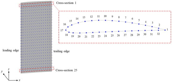
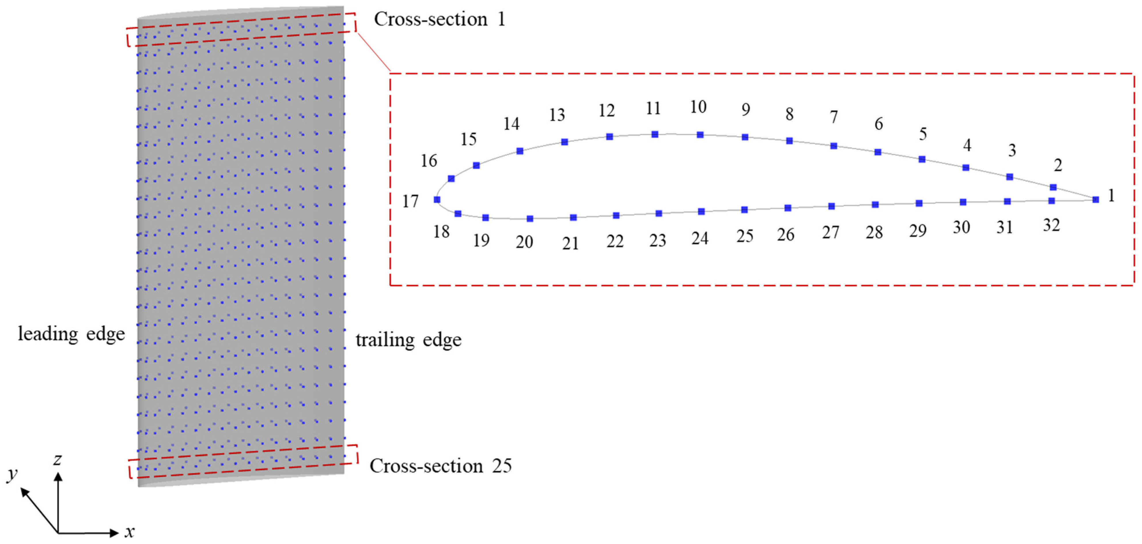
The pressure coefficient C_p on the airfoil surface is selected as the aerodynamic load reconstruction target. Then the sensor data in the real experiment/engineering scenarios is simulated by selecting the data in specific positions from the CFD results. These specific locations, i.e., the location distribution of candidate sensors, are shown in Figure 5, which is, 25 layers are evenly selected along the spanwise direction, and 32 sensors in each layer, resulting a total of 800 sensors.

Figure 5. Schematic of candidate sensor layout. Numbers 1~32 in the enlarged subplot denote the sequential sensor indices at each cross-section.

For each instantaneous field, C_p on the airfoil surface with a resolution of 40 × 156 and the 800 sensor positions are extracted as described above. C_p on the airfoil surface and the sensor positions at the same instant under the same operating condition constitute a data sample, thus a total of 2808 samples can be used for subsequent training, verification and other procedures. These samples originate from URANS simulations in Section 2.2, with Res and AOAs ranges shown in Figure 3. The dataset is randomly split: 2246 samples (80%) for training, 281 samples (10%) for validation, and the remaining 281 samples (10%) for testing. As a result, each subset is mutually exclusive and all covers the Res and AOAs given in Figure 3. In addition, for clear presentation, C_p distributions on the airfoil surface below will be presented in the form of an expanded diagram in the following, specifically, expanded along the arc lengths, from the trailing edge along the suction surface, through the leading edge, and then to the trailing edge along the pressure surface.

3. Construction of Deep Learning Framework

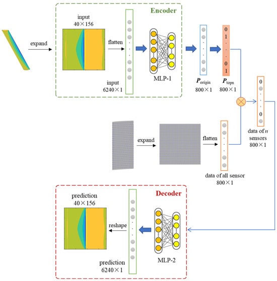
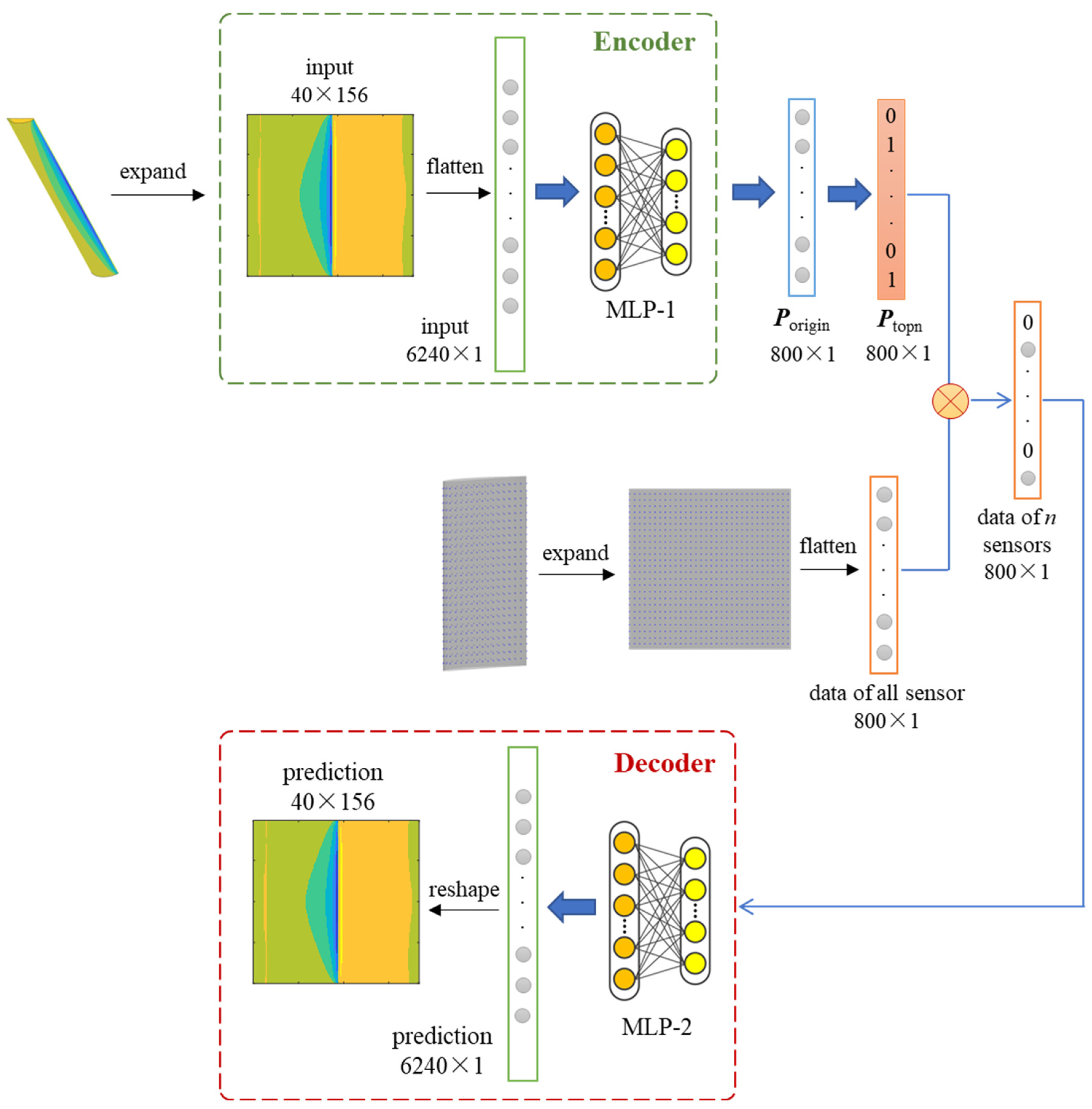
This study proposes a deep learning framework based on autoencoder [40] to automatically determine the optimal sensor placement scheme and reconstruct aerodynamic load of an airfoil, as shown in Figure 6. The algorithm of the framework is described as follows:

Figure 6. Deep learning framework based on autoencoder.

• Encoder:

  (1)

  The input is the original expanded and flattened flow field, which refers to the expansion contour of C_p of the airfoil surface in this study;

  (2)

  After the transformation of MLP-1 section, P_origin, the original probability of each sensor selected is obtained, where MLP refers to Multilayer Perceptron.

• Bottleneck:

  (1)

  Next, P_origin is converted to the top probability matrix P_topn, that is, the data of the first n sensors with the highest probability is set to 1, and the rest positions are set to 0. n in this paper donates for the number of sensors used (selected);

  (2)

  Then a linear combination of all sensor monitoring data and P_topn is carried out, so that only the monitoring data of the selected n sensors can be transferred.

• Decoder: the data is transferred to MLP-2 section, and the predicted flow field can be achieved.
• The loss function is the difference between the predicted flow field and the input flow field.
• In the field reconstruction phase, the model has been trained in advance, so only the decoder is needed. At this time, it has been determined which sensors to select, so the flow field can be reconstructed only by the monitoring data of the n selected sensors.

All input features are normalized to the standard normal distribution before the input layer according to Equation (4), and recovered after the calculation at the output layer. For each data point (pixel) the relative error e_r is defined as

$$e_r={\displaystyle \frac{\left|\widehat{C_p}-C_p\right|}{\left|C_p\right|+1\times {10}^{-30}}}\text{×}100\%,$$

(4)

where $\widehat{C_p}$ is the predicted result; a minimum value of 1 × 10⁻³⁰ is added to the denominator to prevent errors of division by zero. The loss function loss is strictly defined as the average of the absolute values of e_r on all data points of all samples, that is, the average of the relative error point by point, as presented in the following formula:

$$loss={\displaystyle \frac{1}{N_1\times N_2}}{\displaystyle {\sum }_{j=1}^{N_2}}{\displaystyle {\sum }_{i=1}^{N_1}}\left|{e_r}_{i,j}\right|,$$

(5)

where i is the pixel number of the flow field; j refers to the number of samples; N₁ is the total number of pixels in each field (each sample); and N₂ denotes for the number of samples on the dataset.

The mini batch method is adopted with a batch size of 32. As to the optimization algorithm, adaptive momentum estimation algorithm (Adam) is selected and the learning rate set as 1 × 10⁻⁵. Activation functions such as Rectified Linear Unit (ReLU) are applied for all layers except for the output layer. Influence of different activation functions on model performance will also be analyzed in the next section.

4. Results and Discussions

In this section, the training and analysis are carried out under the condition of given 800 candidate sensor positions and the number of sensors to be selected n = 50. The results are described in Section 4.1 and Section 4.2. Trainings are divided into two rounds: in the first round, the specific selected position of sensor is undecided and will be determined by deep learning; in the second round, the specific position of the sensor has been selected, which is obtained by averaging the sensor position distributions obtained from each training sample in the first round. Therefore, only the decoder shown in Figure 6 needs to be trained. The effect of n will be discussed in Section 4.3. These works, including the construction of framework and subsequent training and verification, are carried out by using Python 3.7, PyTorch 1.9.1 and NumPy 1.21.6.

4.1. First Round of Training at n = 50 When Sensor Location Undetermined

4.1.1. Influence of Node Distribution and Activation Functions on Model Performance

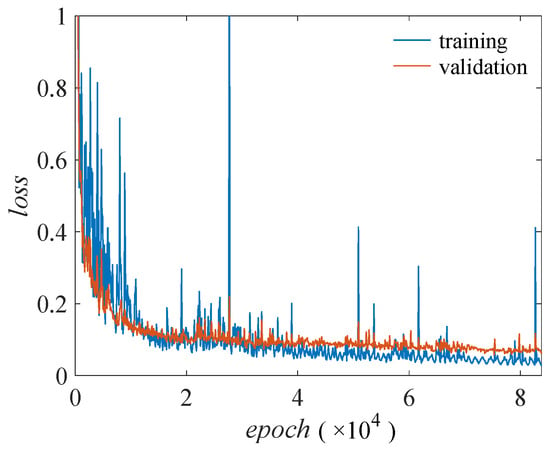
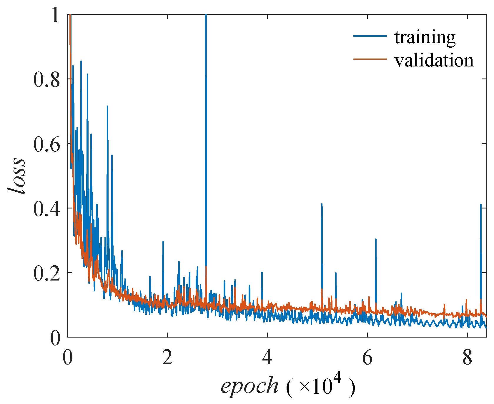
Firstly, the influence of node distributions in the MLP part is analyzed. ReLU is adopted as the activation function besides the output layer. Table 3 shows the training results, in which the node distribution of MLP-2 in the decoder is the same as that of MLP-1 segment in encoder, so only node distribution of MLP-1 is presented for concise. The model size in the table refers to the disk size of the model parameter file. loss vs. epoch for Case 3 is shown in Figure 7 as an example.

Table 3. Node distributions and training results.

Model Name	Node Distribution of MLP-1	Activation Function	Model Size (MB)	Training Loss	Validation Loss
Case 1	100, 100, 100	ReLU	5.55	0.0549	0.0932
Case 2	200, 200, 200	ReLU	11.30	0.0497	0.0924
Case 3	200, 200, 200, 200, 200	ReLU	12.00	0.0279	0.0613
Case 4	200, 200, 200, 200, 200, 200, 200	ReLU	12.60	0.0348	0.0639
Case 5	200, 200, 200, 200, 200, 200, 200, 200, 200, 200, 200	ReLU	13.80	0.0385	0.0680

Figure 7. loss vs. epoch for Case 3.

It can be seen from Table 3 and Figure 7 that the training loss and verification loss basically decreased with the increase in epoch, and training loss occasionally appeared burr, which may be caused by the complexity of the model. In addition, although the validation loss was slightly higher than the training loss in the whole training process, the amplitude was small, and the validation loss did not increase at the later training stage. Therefore, there was no significant overfitting, and no regularization or other techniques to suppress overfitting were used. After training 83,800 epochs, loss did not decrease and the training stopped. From the perspective of model size, the training loss first decreased and then increased with the model size. Case 3 with a model size of 12 MB achieved the minimum loss in both the training set and the validation set, which were 0.0279 and 0.0613, respectively. As a result, the node distribution as shown in Case 3 is adopted in the following, namely, nodes in the MLP segment of encoder and decoder are: 200, 200, 200, 200, 200.

Next, the influence of activation function on the model performance is studied. Different activations functions are set based on Case 3. Table 4 reported the settings and the training results, which demonstrated that ReLU helped to acquire the minimum loss. Accordingly, the activation function was set as ReLU in the subsequent research of this paper.

Table 4. Activation functions and training results.

Model Name	Node Distribution of MLP-1	Activation Function	Training Loss	Validation Loss
Case 3	200, 200, 200, 200, 200	ReLU	0.0279	0.0613
Case 6	200, 200, 200, 200, 200	Leaky ReLU	0.0534	0.0988
Case 7	200, 200, 200, 200, 200	Hyperbolic Tangent (Tanh)	0.0819	0.1027
Case 8	200, 200, 200, 200, 200	Parametric ReLU (PReLU)	0.0405	0.0652
Case 9	200, 200, 200, 200, 200	Exponential Linear Unit (ELU)	0.0558	0.0722
Case 10	200, 200, 200, 200, 200	Mish	0.0712	0.1148
Case 11	200, 200, 200, 200, 200	Gaussian Error Linear Unit (GELU)	0.0463	0.0691
Case 12	200, 200, 200, 200, 200	Scaled Exponential Linear Unit (SELU)	0.0911	0.1112
Case 13	200, 200, 200, 200, 200	Sigmoid Linear Unit (SiLU)	0.0717	0.0909

4.1.2. Analysis of Selected Sensor Distribution

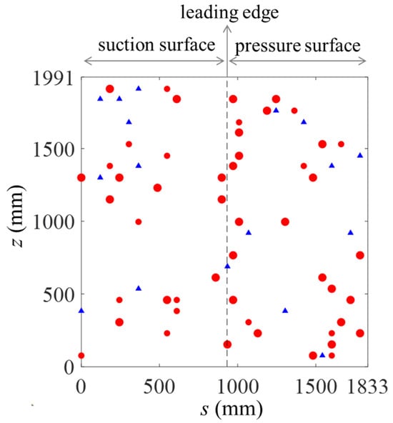
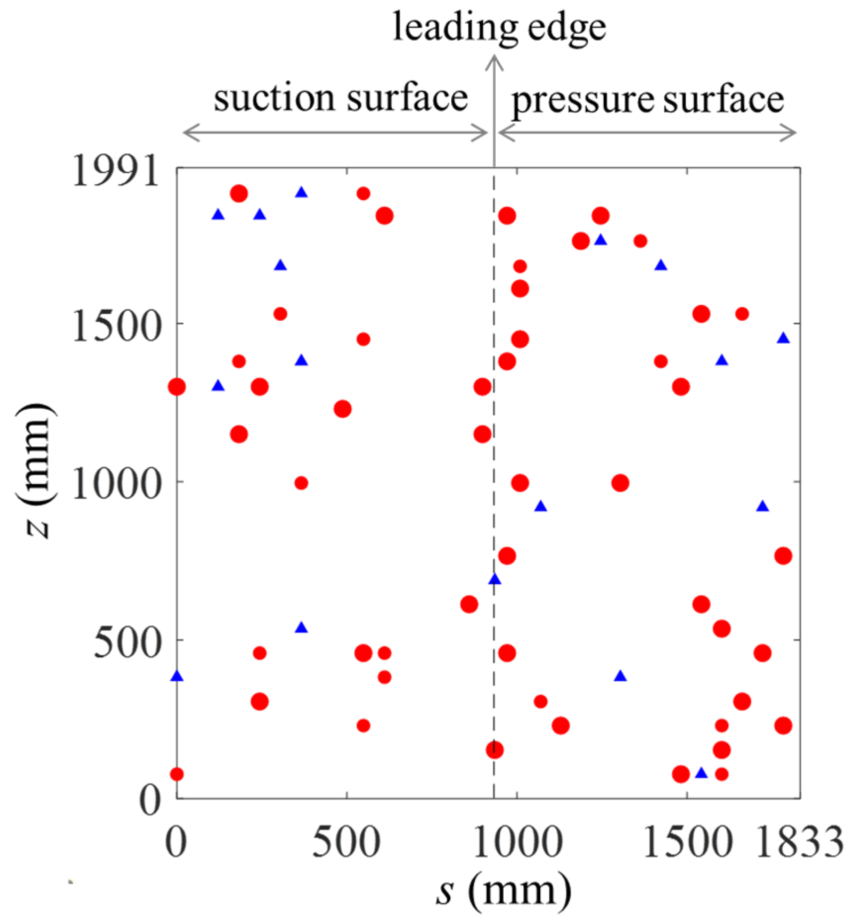
Figure 8 shows the averaged sensor distribution obtained on the training set of Case 3 in the form of an expanded graph. Given that P_topn obtained by each sample is not exactly the same, the sensor selection probability obtained by averaging is a value between 0 and 1. Sixty-seven positions which have been selected are illustrated in the figure. The size of the circles is scaled by the selection probability; therefore, the positions with maximum circles indicate that the selection probability is 1, and the probability of the smaller circle is between 0 and 1. Among the 67 positions provided, the first 50 sensor positions with the highest probability are displayed in red solid circles and are used as the selected sensors in the next session, while the last 17 sensor positions with lower probabilities are displayed in blue solid triangles.

Figure 8. Selected sensor distribution of Case 3.

It can be seen from the figure that:

• There are many high-probability sensors distributed near the leading edge, and they are more concentrated near the leading edge on the pressure side. This may be due to the fact that NACA 4412 is a thin airfoil, and the samples in this study cover a wide range of AOA (from −20° to 25°). Flow separations occur in the leading-edge region in many flow conditions; therefore, the model learned that more sensors need to be arranged in the flow separation region to obtain a better reconstruction of aerodynamic parameters.
• From the point of view of the suction surface and pressure surface, the sensor distribution density is close on both sides of the airfoil. This is due to the reason that although NACA 4412 is asymmetric, the operating condition covers the positive and negative AOAs with similar values, resulting in the close probability of flow separation on the suction surface and pressure surface.
• The spatial distribution of the selected sensors in the spanwise direction is relatively uniform. The upper and lower boundaries of the computational domain are restricted walls. Hence, the flow field has a large variation gradient in the spanwise direction under the conditions with large range of high Res and large AOAs.

4.2. Second Round of Training at n = 50 When Sensor Location Determined

4.2.1. Analysis on Training Results

As mentioned above, the sensor placement is determined by Section 4.1; only the decoder shown in Figure 6 needs to be trained accordingly. After 80,000 epochs, the average loss was 0.0279 in the training set, 0.0659 in the validation set, and 0.0604 in the test set.

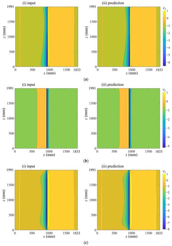
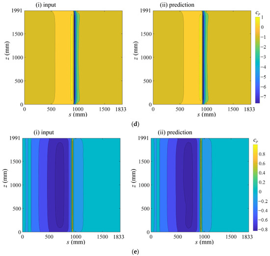
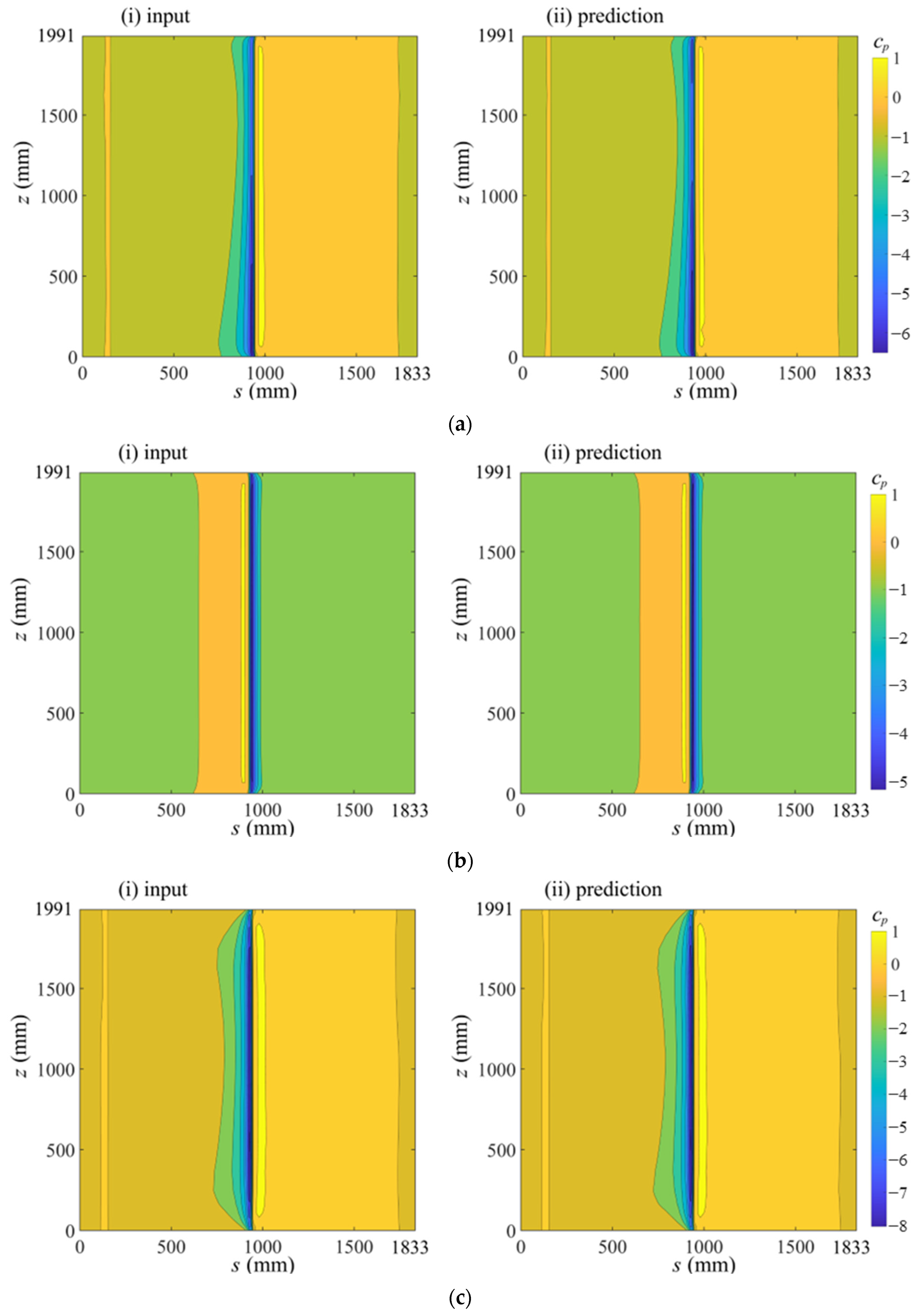
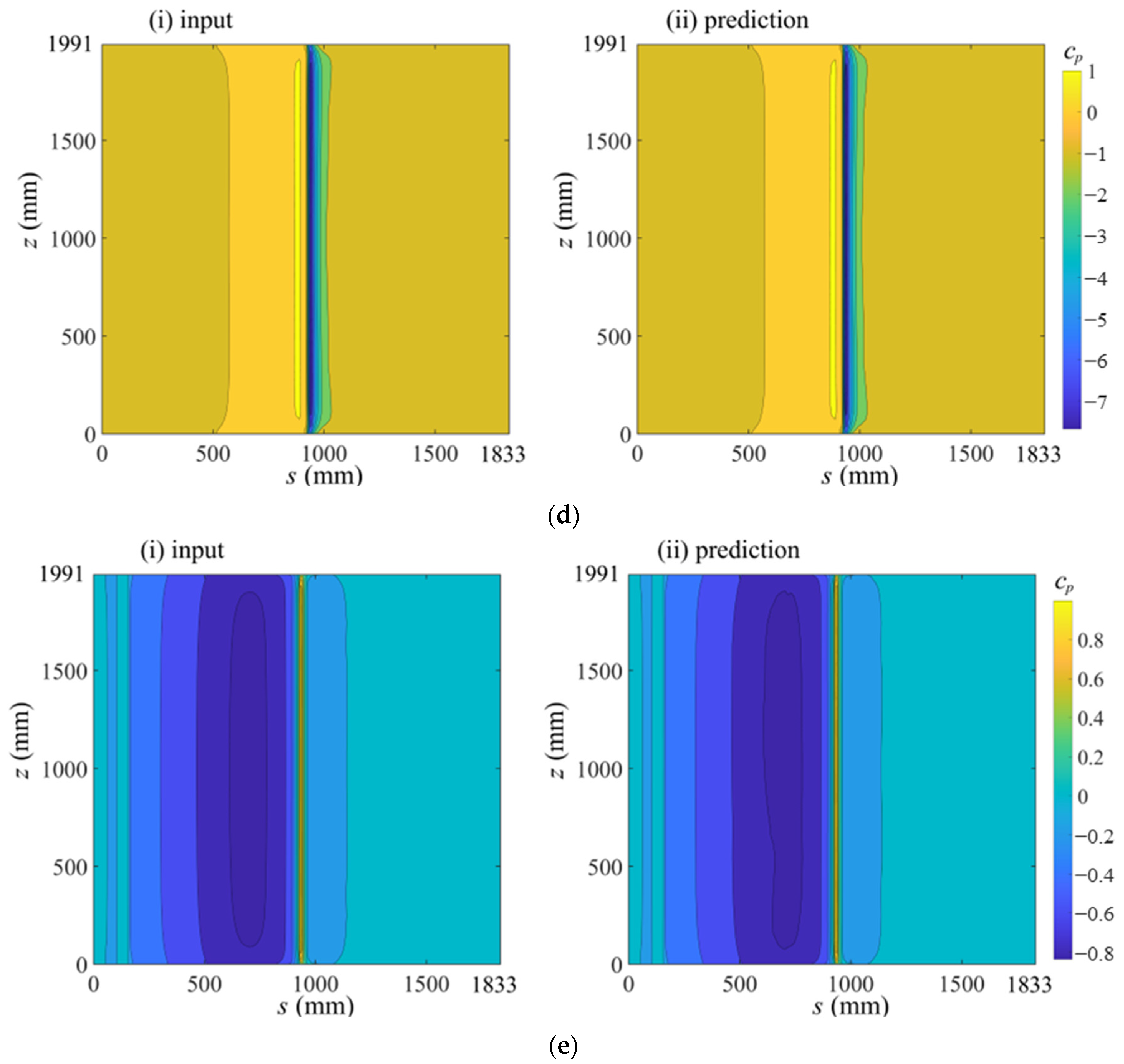
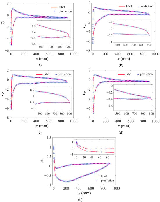
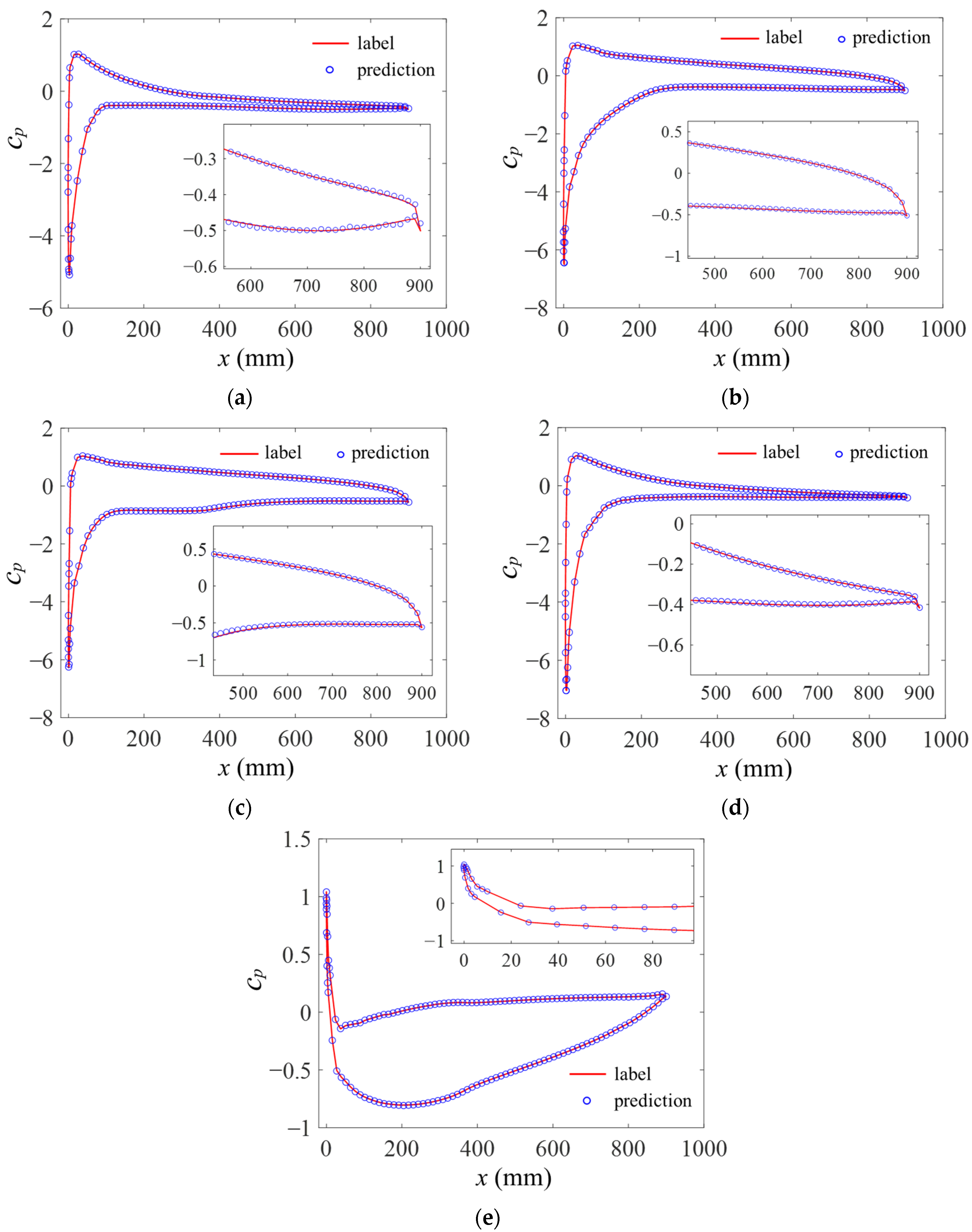
Figure 9 shows comparison of C_p contour between the prediction and the input under 5 typical operating conditions in the test dataset, and these five conditions are also marked in the operating condition diagram (Figure 3). The results demonstrate that the model trained in this section can predict the aerodynamic loads on the airfoil surface well, whether it is under the condition of large or small Re, positive or negative AOA. The prediction accuracy is also good near the leading edge and near the upper and lower walls where the aerodynamic loads change drastically. Overall, high-precision reconstructions of the upper and lower asymmetry and the spatial three-dimensional placement characteristics of the aerodynamic loads are achieved.

Figure 9. Comparison of C_p contour between the prediction and the input under typical operating conditions in the test dataset. (a) Condition A: Re = 1.45 × 10⁶, AOA = −16.61°, t = 1.208 s, loss = 0.0082; (b) Condition B: Re = 1.51 × 10⁶, AOA = 22.73°, t = 0.048 s, loss = 0.0534; (c) Condition C: Re = 1.64 × 10⁵, AOA = 24.07°, t = 1.208 s, loss = 0.0338; (d) Condition D: Re = 2.65 × 10⁵, AOA = −19.10°, t = 0.488 s, loss = 0.0181; (e) Condition E: Re = 8.38 × 10⁵, AOA = 1.31°, t = 0.2 s, loss = 0.1080.

Figure 10 presents a comparison between the input and predicted C_p distributions at the 5% height section under typical operating conditions. Figure 10a,d show the results corresponding to similar negative AOA with the Res differing by one order of magnitude. It can be observed that the overall agreement is satisfactory, with only minor discrepancies near the trailing edge. Figure 10b,c illustrate the results under similar positive AOA, where the Res also differ by one order of magnitude. Combined with Figure 10e, which corresponds to a near-zero AOA, it is evident that the predicted values agree well with the input data.

Figure 10. Comparison of the input and predicted C_p distribution at 5% height section under typical operating conditions. (a) Condition A; (b) Condition B; (c) Condition C; (d) Condition D; (e) Condition E.

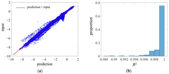
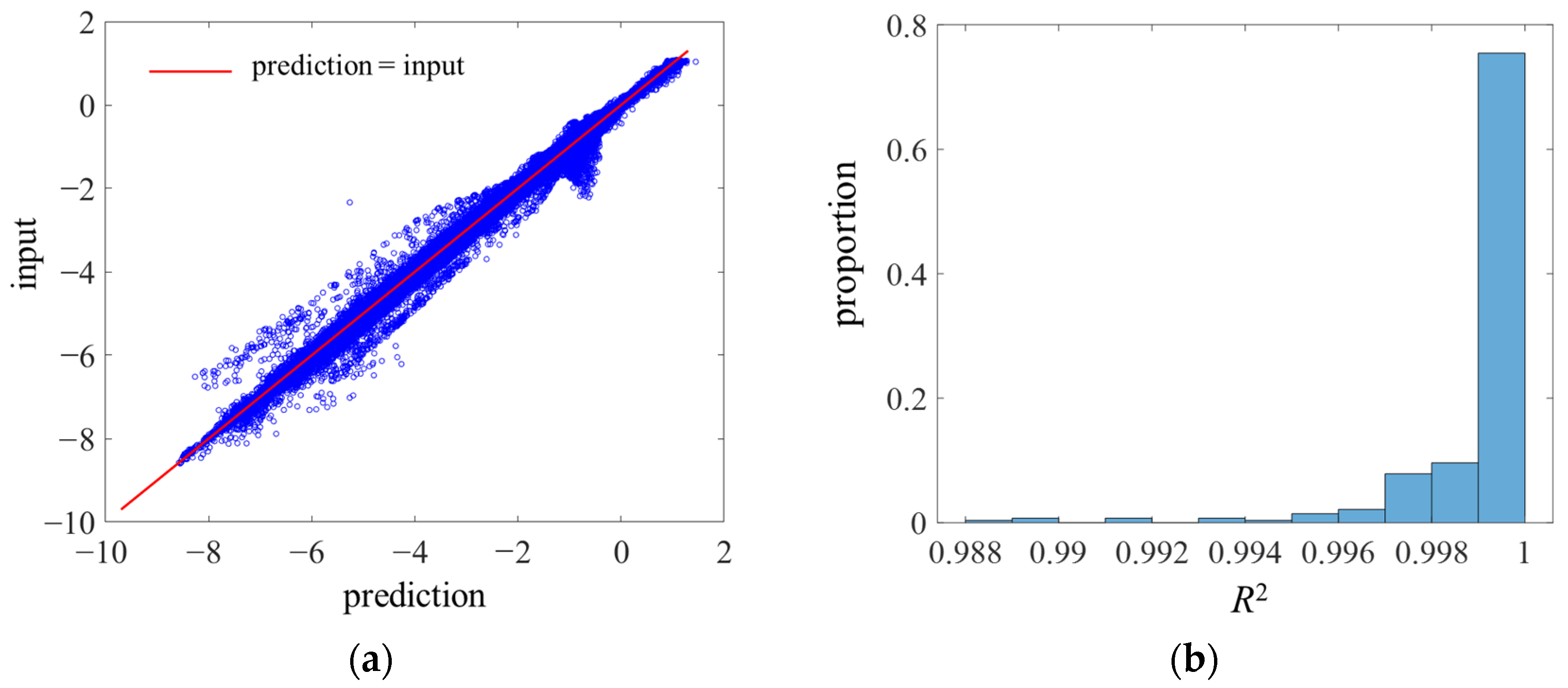
Figure 11 presents a comparison between the predicted values and the input labels for all samples in the test set, together with the histogram of R², where R² denotes for the coefficient of determination based on the fitted line “$\widehat{C_p}$ = $C_p$”. It can be observed that most predictions are in good agreement with the input values on the test set, with an average R² of 0.9990. This further demonstrates that the autoencoder model proposed in this work can effectively reconstruct the aerodynamic loads on the airfoil surface.

Figure 11. Scatter of input and prediction and proportion of R² for all data points in the test dataset. (a) Scatter of input and prediction; (b) Proportion of R².

To account for high-dimensional information such as the spatial distribution characteristics of the flow field, the structural similarity index measure [41] (SSIM) is introduced here, as defined in Equation (6), to overcome the limitation that e_r and loss metrics cannot quantify the structural similarity of flow field distributions:

$$SSIM={\displaystyle \frac{\left(2E_{C_p}{E}_{\widehat{C_p}}+A_1\right)\left(2D_{C_{p,}\widehat{C_p}}+A_2\right)}{\left({E_{C_p}}^2+{E_{\widehat{C_p}}}^2+A_1\right)\left({D_{C_p}}^2+{D_{\widehat{C_p}}}^2+A_2\right)}},$$

(6)

Here, $E_{C_p}$ denotes the mean value of C_p obtained from CFD results, $E_{\widehat{C_p}}$ is the mean value of the predicted field $\widehat{C_p}$, $D_{C_{p,}\widehat{C_p}}$ represents the covariance between C_p and $\widehat{C_p}$, and ${D_{C_p}}^2$ and ${D_{\widehat{C_p}}}^2$ are the variances of C_p and $\widehat{C_p}$, respectively. The constants A₁ = 0.012 and A₂ = 0.032 are adopted to avoid division by zero. SSIM ranges from −1 to 1, where a higher value indicates higher similarity. A value of 1 denotes perfect similarity, 0 indicates no similarity, and negative values represent dissimilarity. Statistical results show that the deep learning model employed in this study achieves an average SSIM of 0.9688 on the test set. This confirms that the proposed method can effectively capture the spatial similarity between the predicted flow field and the input CFD field, and also validates its prediction capability for highly nonlinear flow fields.

4.2.2. Comparisons with Grid Placement Methods

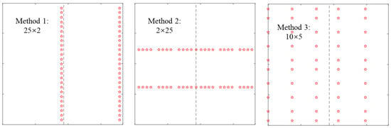
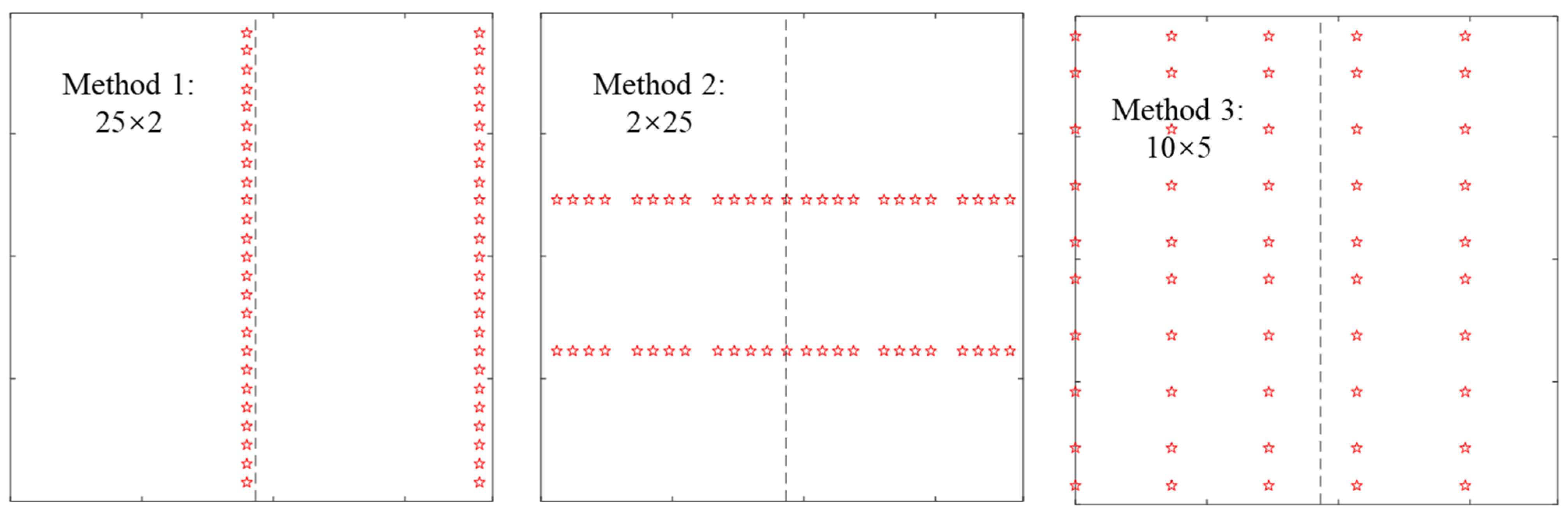
To further evaluate the effectiveness of the optimal sensor placement method and the aerodynamic load reconstruction approach proposed in this study, three common manual sensor layout schemes are constructed in this section based on the characteristics of the 3D airfoil, with a given number of n = 50. These grid placement schemes are illustrated in Figure 12, and the network is trained following similar procedures as in Section 4.2.1. The comparisons under different evaluation metrics are listed in Table 5.

Figure 12. Grid placement methods of sensors when n = 50. The dotted line represents the leading edge, which is the same as Figure 8.

Table 5. Comparisons of reconstruction metrics in test dataset between different placement methods when n = 50.

Metric	Placement Method
	Autoencoder	Grid Placement Method 1	Grid Placement Method 2	Grid Placement Method 3
loss	0.0604	0.0913	0.0793	0.0710
SSIM	0.9688	0.9605	0.9579	0.9656
R2	0.9990	0.9985	0.9982	0.9987
proportion of data points with |er| < 5%	84.18%	76.83%	78.10%	81.99%

It can be observed that Grid Placement Method 1 and Grid Placement Method 2 focus on sensor arrangement along the spanwise and the arc-length direction, respectively, both of which yield relatively poor prediction performance. The loss is 51.2% and 31.2% higher than that of the autoencoder method, respectively, indicating that neither layout can adequately capture the key information of the flow field. Grid Placement Method 3 emphasizes spatially uniform placement, and its performance is significantly improved compared with Grid Placement Methods 1 and 2. Nevertheless, its loss is still 17.5% higher than that of the autoencoder method, and it is inferior to the autoencoder method in three metrics: SSIM, R², and the proportion of data points with |e_r| < 5%. These results further verify the effectiveness of the deep learning framework proposed in this study.

4.3. Influence of Number of Selected Sensors on Model Performance

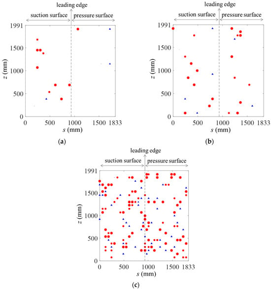
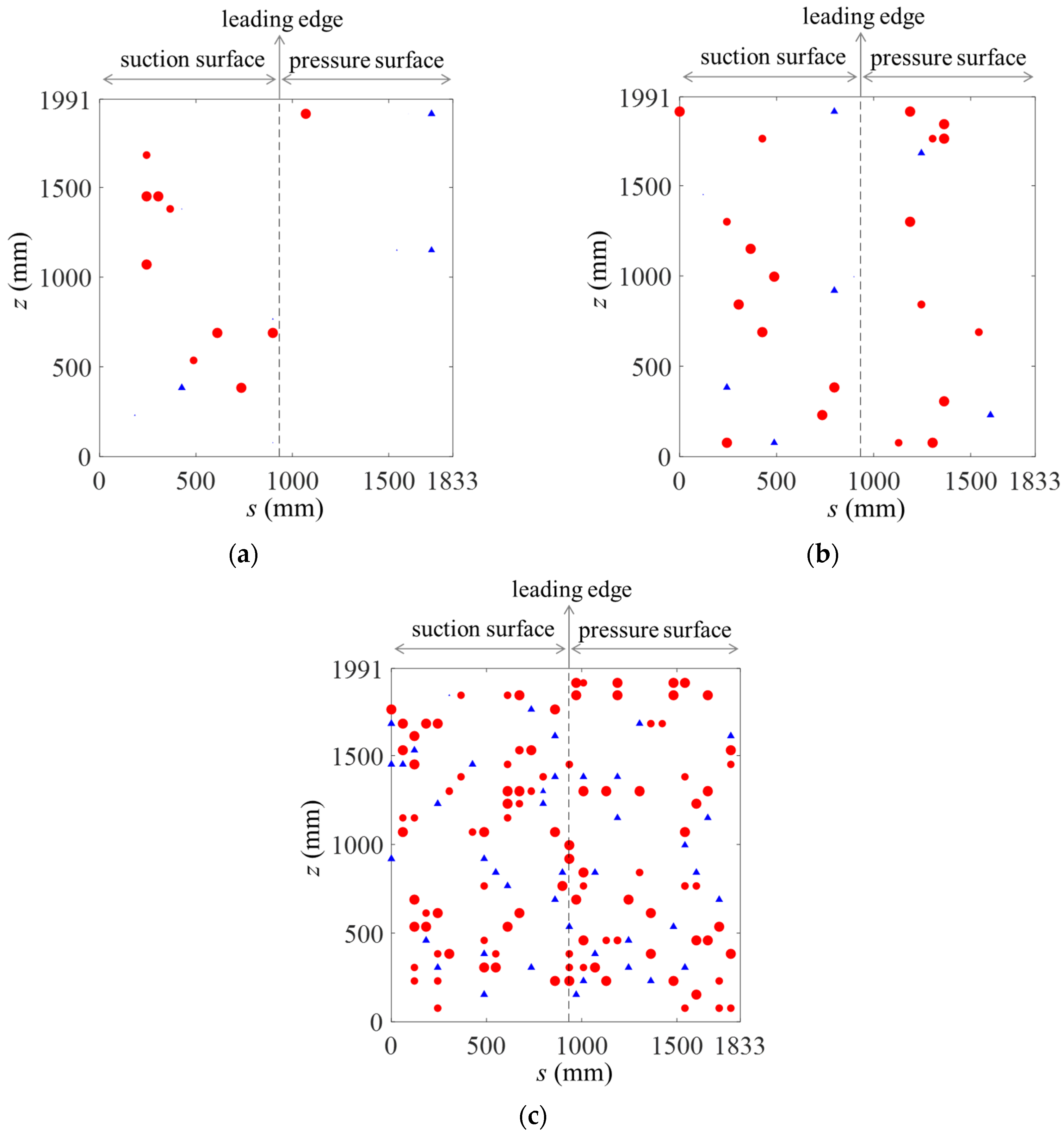
In this section, training is performed with different numbers of selected sensors, i.e., n = 10, 20, 100. The network architecture, settings, and training procedures are identical to those described in Section 4.1 and Section 4.2. The loss and other metrics are summarized in Table 6, and the results of n = 50 from the previous section are also listed for comparison. The corresponding sensor position placements are presented in Figure 13, where the meaning of the symbol sizes and shapes is consistent with that in Figure 8 of Section 4.1.2. For n = 10, a total of 19 sensor locations were selected across all samples, among which six locations exhibited very low selection probabilities (below 0.1), with the minimum value as low as 0.0018. Thus, only 13 distinct points are clearly visible in Figure 13a. For n = 20 and n = 100, there were 28 and 142 unique sensor locations selected over all samples, respectively.

Table 6. Effect of n on model performance.

Metric	n
	10	20	50	100
loss	0.0862	0.0662	0.0604	0.0578
SSIM	0.9555	0.9650	0.9688	0.9701
R2	0.9981	0.9987	0.9990	0.9991
proportion of data points with |er| < 5%	77.06%	81.12%	84.18%	84.74%

Figure 13. Sensor placement obtained through training. (a) n = 10; (b) n = 20; (c) n = 100.

When n = 10, the sensors selected are concentrated on the suction surface of the airfoil, and the model performance is relatively poor at this time, with the loss increasing to 0.0862. Additionally, the proportion of data points with |e_r| < 5% rises by 45% compared with the case of n = 50, indicating that an insufficient number of sensors cannot accurately capture flow field information. With the increase in the number of sensors, the model’s performance in reconstructing aerodynamic parameters is improved. For n = 20, n = 50, and n = 100, the loss is reduced by 23.3%, 29.9%, and 32.9% respectively compared with the case of n = 10. However, when n > 50 and continues to increase, the improvement in model performance is limited. Therefore, the practical determination on n requires a trade-off between the constraint on the number of sensors and the accuracy of reconstruction performance. It is worth noting that the SSIM values and R² under the four given sensor quantities are relatively close. For example, the SSIM for n = 100 is only 1.5% higher than that for n = 10, indicating that the flow structure similarity index SSIM and R² are not sensitive to the number of sensors selected.

In addition, it can be seen from Table 5 and Table 6 that for n = 10, the loss and the proportion of data points with |e_r| < 5% obtained by the autoencoder-based method are superior to those obtained by Grid Placement Method 1 with n = 50; for n = 20, the loss and the proportion of data points with |e_r| < 5% obtained by the autoencoder-based method are superior to those obtained by Grid Placement Method 3 with n = 50. These indicate that under the same reconstruction accuracy, the autoencoder-based method proposed in this study can save at least 60% to 80% of the number of sensors compared with manual placement methods, implying significant engineering application value.

4.4. Discussions on Advantages and Limitations

As can be observed from the above results, the proposed framework efficiently addresses optimal sensor placement and flow field reconstruction and exhibits excellent generalizability. It is applicable not only to airfoil flow presented in this work but also to more complex scenarios such as rotating machinery, multiphase flow and phase-change flow, though further validation is required for these challenging cases. In addition, the flow fields to be predicted, including pressure coefficient, velocity, temperature and pressure fields (or their combinations), are treated as images in this study. In practical applications, this approach can use CFD or experimental data with flexible selection freedom. This allows adopting well-established techniques from computer vision. For instance, the MLP module can be replaced with CNN and transposed CNN architectures, making the framework more flexible and lightweight.

Nevertheless, with the growing application of artificial intelligence and CFD in engineering, physics-embedded frameworks have been increasingly adopted for optimal sensor placement. Representative approaches such as PINNs [42,43] integrate the Navier–Stokes equations into sensor placement and flow field reconstruction, enforcing physical constraints on predicted velocity and pressure fields. Unlike these methods, the proposed framework does not embed governing differential equations, leading to insufficient physical consistency. However, it outperforms in flexibility and generalizability, as discussed previously. Future work will combine the strengths of both frameworks to achieve complementary advantages.

Moreover, this study has several limitations. Although the dataset covers a wide range of angles of attack and Reynolds numbers, as well as different stages of unsteady flow evolution, uniform and constant inlet boundaries are adopted to approximate free-stream turbulence. The present samples do not include inflow conditions with unsteady, non-uniform and strong fluctuations such as the atmospheric boundary layer. Such inflows may increase pressure gradients and expand flow separation and vortex regions, which could affect the performance and robustness of the proposed framework. Furthermore, during the establishment of the URANS database in Section 2.2, developing transient flow fields were selected to enrich dataset diversity, while quasi-steady solutions were excluded from the dataset, as evidenced in Figure 4. Distinctions inherently exist between evolving transient flow data and quasi-steady solutions, which may influence the accuracy and robustness of the proposed model. Further investigations will be carried out in future work.

Additionally, the database in this work is established based on URANS simulations, which has two major limitations. First, although the database covers wide ranges of Reynolds numbers and angles of attack with numerous snapshots of transient flow evolution, URANS filters out high-frequency turbulent fluctuations via Reynolds averaging. Combined with the inherent limitations of turbulence models, it yields larger errors than high-fidelity methods such as Large Eddy Simulation and Direct Numerical Simulation, especially for complex flows. Second, CFD adopts idealized boundary conditions and cannot fully reproduce real experimental factors including environmental disturbances and wall roughness. Actual measured data contains more noise and complex flow features, which may complicate sensor placement and reduce reconstruction accuracy. Further research using experimental data will be conducted in the future.

5. Conclusions and Prospectives

In this paper, the pressure coefficient of a three-dimensional airfoil with finite span is taken as the key reconstruction parameter. A transient flow field database covering different Res and wide range of AOAs is constructed using CFD method. A deep learning network architecture based on an autoencoder is proposed to conduct research on the optimal layout of sensors and the subsequent aerodynamic load reconstruction. The main conclusions are drawn as follows:

(1)

When the network model reaches its optimal state, the node configuration of the MLP in both the encoder and decoder is determined as 200, 200, 200, 200, 200. Either an excessive or insufficient number of nodes will hinder the accurate characterization of the three-dimensional airfoil flow field dataset adopted in this study. Among various activation functions, ReLU achieves the best performance. Its minimum training loss is 0.0279, which is at least 45% lower than those of other activation functions, and the minimum validation loss is 0.0613, representing a reduction in no less than 6% compared with the alternatives. The optimal sensor layout presents distinct characteristics: sensors are densely arranged near the airfoil leading edge and distributed relatively uniformly along the spanwise direction.

(2)

Evaluated by loss, R², e_r, and SSIM, the model exhibits superior performance when the number of sensors n = 50. Under this condition, the average loss values for the training, validation and test sets are 0.0279, 0.0659 and 0.0604 respectively, with R² = 0.9990 and SSIM = 0.9688. The proposed model can effectively realize automatic optimal sensor placement and reconstruct aerodynamic loads on the surface of three-dimensional airfoils with high precision. When n < 50, the model’s prediction performance improves as the number of sensors increases, while only marginal performance improvement can be observed when n > 50.

(3)

With the same number of sensors (taking n = 50 as an example), the reconstruction performance of the proposed deep learning framework is quantified by loss = 0.0604, R² = 0.9990 and SSIM = 0.9688. By contrast, the optimal results of common manual sensor placement are loss = 0.0710, R² = 0.9987 and SSIM = 0.9656. The comparison clearly demonstrates that the proposed framework outperforms traditional manual placement methods in terms of aerodynamic load reconstruction accuracy.

(4)

Under the same reconstruction accuracy, the autoencoder-based method proposed in this study can save at least 60% to 80% of the number of sensors compared with manual placement methods.

In this study, data at specific positions are selected from the airfoil aerodynamic load data calculated by CFD to simulate sensor data, and the proposed autoencoder-based deep learning model can realize the optimal layout of sensors and high-precision reconstruction of flow fields, which has significant engineering application value. Although the proposed method shows good flexibility and generalizability in sensor placement and flow field reconstruction, it still has limitations such as the absence of physical constraints and oversimplified data compared with real engineering data. These issues will be further investigated in future work.

References

- Scavella, P.; Paolillo, G.; Greco, C.S. Deep reinforcement learning-based airfoil design and optimization: An aerodynamic analysis. Aerosp. Sci. Technol. 2025, 167, 110638. [Google Scholar] [CrossRef] [Scilit]
- Bhattacharjee, D.; Klose, B.; Jacobs, G.B.; Hemati, M.S. Data-driven selection of actuators for optimal control of airfoil separation. Theor. Comput. Fluid Dyn. 2020, 34, 557–575. [Google Scholar] [CrossRef] [Scilit]
- Hollenbeck, A.C.; Grandhi, R.; Hansen, J.H.; Pankonien, A.M. Sparse flow sensor placement optimization for flight-by-feel control of 2D airfoils. AIAA J. 2024, 62, 3803–3812. [Google Scholar] [CrossRef] [Scilit]
- Gunder, T.; Sehlinger, A.; Skoda, R.; Mönnigmann, M. Sensor placement for reduced-order model-based observers in hydraulic fluid machinery. IFAC-PapersOnLine 2018, 51, 414–419. [Google Scholar] [CrossRef] [Scilit]
- Karnik, N.; Abdo, M.; Estrada-Perez, C.; Yoo, J.; Cogliati, J.; Skifton, R.; Calderoni, P.; Brunton, S.; Manohar, K. Constrained optimization of sensor placement for nuclear digital twins. IEEE Sens. J. 2024, 24, 15501–15516. [Google Scholar] [CrossRef] [Scilit]
- Luo, X.; Kareem, A.; Yoo, S. Optimal sensor placement for reconstructing wind pressure field around buildings using compressed sensing. J. Build. Eng. 2023, 75, 106855. [Google Scholar] [CrossRef] [Scilit]
- Akhtar, I.; Borggaard, J.; Burns, J. Computing functional gains for designing more energy-efficient buildings using a model reduction framework. Fluids 2018, 3, 97. [Google Scholar] [CrossRef] [Scilit]
- Fei, J. Optimal arrangement of pressure monitoring points in water supply network based on intelligent optimization algorithm. In Hydraulic Structure and Hydrodynamics; Lecture Notes in Civil Engineering; Springer: Singapore, 2025; pp. 451–461. [Google Scholar]
- Nasr, D.; Saad, G. Optimal sensor placement using a combined genetic algorithm—Ensemble Kalman Filter framework. ASCE-ASME J. Risk Uncertain. Eng. Syst. Part A Civ. Eng. 2016, 3, 04016010. [Google Scholar] [CrossRef] [Scilit]
- Shi, S.; Du, D.; Mercan, O.; Kalkan, E.; Wang, S. A novel data-driven sensor placement optimization method for unsupervised damage detection using noise-assisted neural networks with attention mechanism. Mech. Syst. Signal Process. 2024, 209, 111075. [Google Scholar] [CrossRef] [Scilit]
- Sevart, C.D.; Kim, J.; Wang, Y.; Simac, J.; Kaminsky, A. Optimal sensor placement and aerostructural control using state-consistent reduced-order models. AIAA J. 2025, 63, 4930–4946. [Google Scholar] [CrossRef] [Scilit]
- Hinson, B.T.; Morgansen, K.A. Observability-based optimal sensor placement for flapping airfoil wake estimation. J. Guid. Control Dyn. 2014, 37, 1477–1486. [Google Scholar] [CrossRef] [Scilit]
- Guzmán-Iñigo, J.; Sodar, M.A.; Papadakis, G. Data-based, reduced-order, dynamic estimator for reconstruction of nonlinear flows exhibiting limit-cycle oscillations. Phys. Rev. Fluids 2019, 4, 114703. [Google Scholar] [CrossRef] [Scilit]
- Saito, Y.; Yamada, K.; Kanda, N.; Nakai, K.; Nagata, T.; Nonomura, T.; Asai, K. Data-driven determinant-based greedy under/oversampling vector sensor placement. CMES-Comput. Model. Eng. Sci. 2021, 129, 1–30. [Google Scholar] [CrossRef] [Scilit]
- Kanda, N.; Abe, C.; Goto, S.; Yamada, K.; Nakai, K.; Saito, Y.; Asai, K.; Nonomura, T. Proof-of-concept study of sparse processing particle image velocimetry for real time flow observation. Exp. Fluids 2022, 63, 143. [Google Scholar] [CrossRef] [Scilit]
- Nasr, D.; Saad, G. Sensor placement optimization using Ensemble Kalman Filter and genetic algorithm. In Proceedings of the 5th ECCOMAS Thematic Conference on Computational Methods in Structural Dynamics and Earthquake Engineering (COMPDYN), Crete Island, Greece, 25–27 May 2015; pp. 3296–3308. [Google Scholar]
- Cohen, K.; Siegel, S.; Wetlesen, D.; Cameron, J.; Sick, A. Effective sensor placements for the estimation of Proper Orthogonal Decomposition mode coefficients in von Karman Vortex Street. J. Vib. Control 2004, 10, 1857–1880. [Google Scholar] [CrossRef] [Scilit]
- Kumar, P.; Sayed, Y.M.E.; Semaan, R. Optimized sensor placement using stochastic estimation for a flow over a 2D airfoil with Coanda blowing. In Proceedings of the 7th AIAA Flow Control Conference, Atlanta, GA, USA, 16–20 June 2014. [Google Scholar]
- Sashittal, P.; Bodony, D.J. Data-driven sensor placement for fluid flows. Theor. Comput. Fluid Dyn. 2021, 35, 709–729. [Google Scholar] [CrossRef] [Scilit]
- Barklage, A.; Stradtner, M.; Bekemeyer, P. Sensor placement for optimal aerodynamic data fusion. Aerosp. Sci. Technol. 2024, 155, 109598. [Google Scholar] [CrossRef] [Scilit]
- Yang, L.; Zhu, M. Review on the status and development trend of AI industry. In Proceedings of the IEEE 4th International Conference on Cloud Computing and Big Data Analysis (ICCCBDA), Chengdu, China, 12–15 April 2019. [Google Scholar]
- Jean-Claude, K.K. A comprehensive overview of artificial intelligence. In Proceedings of the 2nd International Conference on Advances in Computing & Information Technologies (CACIT 2022), Sydney, Australia, 22–23 December 2022; pp. 173–194. [Google Scholar]
- Kaya, M.N.; Büyükzeren, R.; Pektaş, A. Performance prediction of air source heat pumps under cold and hot ambient temperatures using ANFIS and ANN models. Symmetry 2025, 17, 1728. [Google Scholar] [CrossRef] [Scilit]
- Semaan, R. Optimal sensor placement using machine learning. Comput. Fluids 2017, 159, 167–176. [Google Scholar] [CrossRef] [Scilit]
- Kelmar, T.; Chierichetti, M.; Davoudi Kakhki, F. Optimization of sensor placement for modal testing using machine learning. Appl. Sci. 2024, 14, 3040. [Google Scholar] [CrossRef] [Scilit]
- Deng, Z.W.; He, C.X.; Liu, Y.Z. Deep neural network-based strategy for optimal sensor placement in data assimilation of turbulent flow. Phys. Fluids 2021, 33, 025119. [Google Scholar] [CrossRef] [Scilit]
- Paris, R.; Beneddine, S.; Dandois, J. Robust flow control and optimal sensor placement using deep reinforcement learning. J. Fluid Mech. 2021, 913, A25. [Google Scholar] [CrossRef] [Scilit]
- Mons, V.; Chassaing, J.-C.; Sagaut, P. Optimal sensor placement for variational data assimilation of unsteady flows past a rotationally oscillating cylinder. J. Fluid Mech. 2017, 823, 230–277. [Google Scholar] [CrossRef] [Scilit]
- NVIDIA PhysicsNeMo Team. NVIDIA PhysicsNeMo. 2026. Available online: https://github.com/NVIDIA/physicsnemo (accessed on 30 May 2026).
- Chandra, A.; Koch, M.; Pawar, S.; Panda, A.; Azizzadenesheli, K.; Snippe, J.; Alpak, F.O.; Hariri, F.; Etienam, C.; Devarakota, P.; et al. Accelerating Porous Media Flow Simulations with Fourier Neural Operators: An Application to Geologic Storage of CO2. Adv. Theory Simul. 2026, 9, e00747. [Google Scholar] [CrossRef] [Scilit]
- Machine Learning for Fluid Dynamics. 2026. Available online: https://ml4fluids2026.github.io/ (accessed on 30 May 2026).
- Coles, D.; Wadcock, A.J. Flying-hot-wire study of flow past an NACA 4412 airfoil at maximum lift. AIAA J. 1979, 17, 321–329. [Google Scholar] [CrossRef] [Scilit]
- Wilcox, D.C. Turbulence modeling for CFD, 3rd ed.; DCW Industries: La Canada, CA, USA, 2006. [Google Scholar]
- Versteeg, H.K.; Malalasekera, W. An Introduction to Computational Fluid Dynamics: The Finite Volume Method, 2nd ed.; Pearson Education Limited: Harlow, UK, 2007; pp. 268–271. [Google Scholar]
- Bulat, P.; Chernyshov, P.; Prodan, N.; Volkov, K. Control of aerodynamic characteristics of thick airfoils at low Reynolds numbers using methods of boundary layer control. Fluids 2024, 9, 26. [Google Scholar] [CrossRef] [Scilit]
- Barth, T.J.; Jesperson, D.C. The design and application of upwind schemes on unstructured meshes. In Proceedings of the AIAA Aerospace Sciences Meeting, Reno, NV, USA, 9–12 January 1989; p. 0366. [Google Scholar]
- ANSYS Inc. ANSYS-CFX: Users Manual Version 19.0, ANSYS: Canonsburg, PA, USA.
- ANSYS Inc. ANSYS-ICEM CFD: Users Manual Version 19.0, ANSYS: Canonsburg, PA, USA.
- McKay, M.; Beckman, R.; Conover, W. A comparison of three methods for selecting vales of input variables in the analysis of output from a computer code. Technometrics 1979, 21, 239–245. [Google Scholar]
- Ackley, D.H.; Hinton, G.E.; Sejnowski, T.J. A learning algorithm for Boltzmann Machines. Cogn. Sci. 1985, 9, 147–169. [Google Scholar] [CrossRef] [Scilit]
- Boudaghi, F.; Waleed, D.; Duffaut Espinosa, L.A. Data reconstruction using smart sensor placement. Sensors 2024, 24, 6008. [Google Scholar] [CrossRef] [Scilit]
- Venianakis, G.; Theodoropoulos, C.; Kavousanakis, M. A physics informed machine learning framework for optimal sensor placement and parameter estimation. Comput. Chem. Eng. 2026, 210, 109652. [Google Scholar] [CrossRef] [Scilit]
- Zhu, Q.; Zhao, Z.; Yan, J. Physics-informed machine learning for surrogate modeling of wind pressure and optimization of pressure sensor placement. Comput. Mech. 2023, 71, 481–491. [Google Scholar] [CrossRef] [Scilit]
Disclaimer/Publisher’s Note: The statements, opinions and data contained in all publications are solely those of the individual author(s) and contributor(s) and not of MDPI and/or the editor(s). MDPI and/or the editor(s) disclaim responsibility for any injury to people or property resulting from any ideas, methods, instructions or products referred to in the content. |
© 2026 by the authors. Licensee MDPI, Basel, Switzerland. This article is an open access article distributed under the terms and conditions of the Creative Commons Attribution (CC BY) license.