


Abstract
An optical lens focuses light and a similar device can be developed to focus surface water waves. A detailed description of such hydrodynamic lenses is given, for which the focusing is induced by shaping the bathymetry of the bottom. Classically, the Luneburg lens uses a specific radial variation of the refractive index. The modified Luneburg lens (MLL) introduces an extra degree of freedom, permitting the focal point to be tuned. It is shown how to design the MLL for water waves, and then its performance is evaluated. Compared with a simple parabolic-shaped mount, the MLL is shown to be free of spherical aberration, resulting in a focus with larger intensity and smaller size of the focal point. Moreover, the focusing properties can be tuned and enhanced thanks to the possibility of changing the position of the focal point. The focusing quality of the MLL is described in all water-depth regimes (covering dispersive and non-dispersive waves) and the focusing of linear and nonlinear waves is revealed experimentally. The option of moving the focal point outside the lens, where the water depth is constant, may be useful when locating devices for harvesting wave energy.
1. Introduction
It is well known that when surface water waves pass across an elevated bathymetry, refraction often results in the amplification of waves behind it [1,2,3,4,5]. This phenomenon can be enhanced by adjusting the bathymetry so as to create a hydrodynamic lens: the focusing of the waves can then be used to increase the harvest efficiency of devices designed to extract power from the waves. A hydrodynamic lens can concentrate waves on a particular focal point by transforming straight crests of incident waves, just like an optical lens. These hydrodynamic lenses have attracted the attention of ocean engineers; they are promising because they might enable the effective utilization of wave energy [6,7], the remaining challenge being to increase the harvest efficiency of the lens.
According to Griffiths and Porter [8], the idea of focusing with underwater lenses was first suggested by Mehlum and Stamnes in 1978. Since then, amplification and focusing of surface water waves by variable bathymetry have been studied in several situations, including gradual changes in depth and abrupt changes in depth (submerged plates); see, for example, [3,8,9,10,11,12,13,14,15,16,17,18]. Based on homogenization theory, the interactions of water waves with lens-like structures made of periodic bottom-mounted vertical cylinders have been investigated in the long-wavelength limit [19,20,21]. New mechanisms for controlling surface water waves, mainly inspired by photonic crystals and metamaterials, have been revealed, such as negative effective gravity [22,23], epsilon-near-zero focusing [24], zero refractive index [25] or reflectionless shifters [26]. Also, Maxwell’s fishpond lens, working for a source point [27] and gradient index media [28], have been studied in the shallow-water limit.
To fix ideas, we can start by considering two-dimensional acoustic waves governed by the Helmholtz equation, , where the refractive index n is specified and is the constant wavenumber in the region where . The lens corresponds to the bounded region where ; for simplicity, take this region to be a disc (r is a plane polar coordinate) and assume that n is a function of r only. The classical Luneburg lens [29,30] corresponds to the choice ; it collects plane waves and focuses them at a point on the circle . This focal point can be moved by using [31]
where is a dimensionless parameter. This defines the modified Luneburg lens (MLL). We are interested in the hydrodynamic analog of this lens. Lenses created using inhomogeneous media have been named ‘gradient index’ (GRIN) devices. They have recently shown interesting properties in many domains of physics [27,32,33,34,35,36,37,38,39].
In this paper, we give a detailed description of the efficiency of a hydrodynamic MLL. We consider surface waves on water of arbitrary (finite) depth: we do not restrict to shallow water waves. Specifically, if is the constant water depth outside the region occupied by the lens and is the wavenumber there, we say that we are in the shallow-water regime if .
In Section 2, the bathymetry profile for the MLL is determined as a function of the water-wave regime. It is shown that the bathymetry profile does not depend on frequency in the shallow-water regime (). For larger values of , the bathymetry profile does depend on the frequency. In Section 3, the propagation of surface water waves over the MLL is analyzed for non-dispersive shallow-water waves. The classical Luneburg lens, for which the focal point lies at the rim of the lens, is studied in Section 3.1 and results are compared with a parabolic-shaped lens in Section 3.2. Then, tunable and improved focusing is presented with the MLL in Section 3.3. In Section 4, the propagation of surface water waves over the MLL is studied in a more general case, without restriction to shallow-water waves. The evolution of the quality of the focusing through a fixed lens is presented as a function of the frequency of the incident wave in Section 4.1. Also optimal focusing of dispersive waves is demonstrated in Section 4.2. Finally, experiments of the focusing of linear and nonlinear waves are presented in Section 5.
2. Bathymetry Profile for the Modified Luneburg Index
2.1. Index of the Luneburg Lens
The classical Luneburg lens is a GRIN lens with a spatially varying refractive index
where r is the radial distance from the lens center and is the radius of the lens [29,30]. Outside the lens (), . The Luneburg lens focuses an incident plane wave on a focal point diametrically opposed to the incident direction at . A modified version of the Luneburg lens enables us to tune the location of the focal point at a distance from the lens center [31]. This modified Luneburg lens (MLL) has given by
with
When (), the focal point lies inside (outside) the lens and when , the MLL reduces to the classical Luneburg lens.
2.2. Application to Water Waves
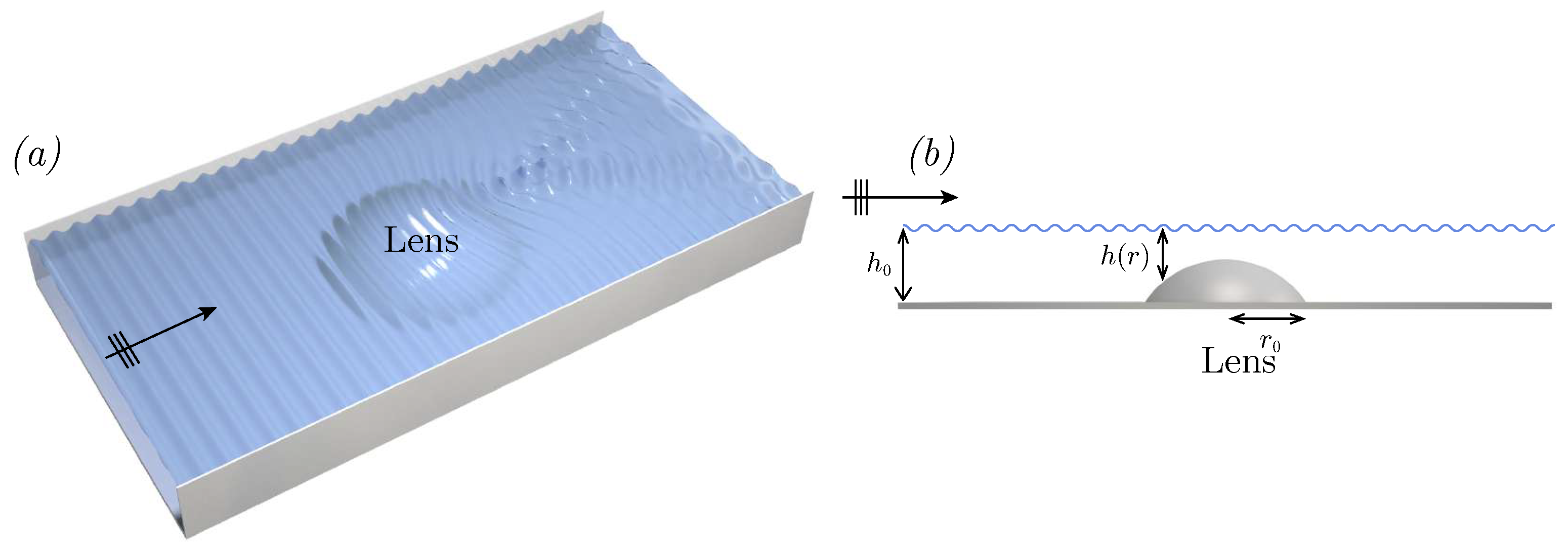
As illustrated in Figure 1, to apply the concept of the GRIN lens to water waves, we can use a varying bathymetry to obtain a varying index. Indeed, water waves are described by the dispersion relation
with the frequency, k the wavenumber, h the local water depth and g the gravity constant. The phase speed is . Outside the lens, the wavenumber is , the constant water depth is and the phase speed is . By definition, the refractive index is ,
Equation (5) shows the dependency of n on the bathymetry through h. It also shows that a correspondence between n and h will depend on the chosen frequency . This contrasts with the case of non-dispersive waves, where the correspondence between n and the inhomogeneity of the medium is obtained independently of the frequency. This also contrasts with the case of dispersive waves with a dispersion relation of the form , leading also to a correspondence being frequency independent; see [36] in the case of flexural waves in elastic plates ( in this context). Coming back to water waves, there are two regimes where . The first regime corresponds to the dispersionless shallow-water limit ( and ), thus . The second regime is the deep water limit ( and ), with , but this is of no interest here: there would be no bathymetry for the waves to feel!
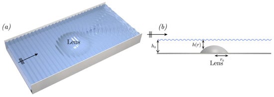
Figure 1.
(Colour online) (a) Top and (b) side views of the configuration.
The analysis presented in the following sections is made as a function of the water wave regime defined by . In fact, we shall consider the water depth to be fixed so that increasing will be equivalent to increasing the frequency. In general, for a given frequency corresponding to a given , the water depth profile h, see Figure 1, can be determined by solving (5) numerically. Fortunately, a good approximate solution of the dispersion relation (see Appendix A) provides an analytical expression for the bathymetry,
The shallow-water case ( and ) leads to significant simplifications, with
where is given by (2).
Thus, the analysis can be divided into two main parts, as follows.
2.3. The Mild Slope Equation
The Luneburg index, and the resulting variation in the bathymetry, only guarantees focusing of rays in the high-frequency limit. At finite frequencies, it makes sense to inspect whether or not the bathymetry produces the expected focusing. To have a hope of a good lensing effect to occur, the lens has to contain many wavelengths, which means . On the other hand, the wave will be sensitive to the bathymetry for moderate values of , say . Combining these two, it follows that the ratio , which means that the bathymetry of the lens is slowly varying. This is good news since it allows us to solve the water wave propagation problem using the Mild Slope Equation (MSE), thus avoiding solving the full three-dimensional problem. The MSE [40] governing the surface wave elevation is
where and is the group velocity,
The MSE can be employed efficiently to predict linear wave propagation over an arbitrary bathymetry and is valid when [41]. Note that many modified and extended forms of the MSE have been proposed [42,43,44,45,46,47,48] to include the effects of wave nonlinearity, seabed slope, wave breaking or bed friction.
When the depth is small compared to the wavelength (), the MSE tends to the linear Shallow Water Equation (SWE),
which clearly recovers the index scaling of (7).
3. The Modified Luneburg Lens in the Shallow-Water Regime
In this part, the focusing properties of the modified Luneburg lens (MLL) are analyzed when the depth is small compared to the wavelength. This is conducted with the SWE (9), which gives non-dispersive wave propagation with . The focusing of surface water waves by the classical Luneburg lens is revealed and improved in comparison with a parabolic conical mount. In addition, the tunability of the MLL in the position of the focal point is demonstrated.
3.1. Classical Luneburg Lens
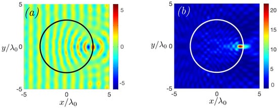
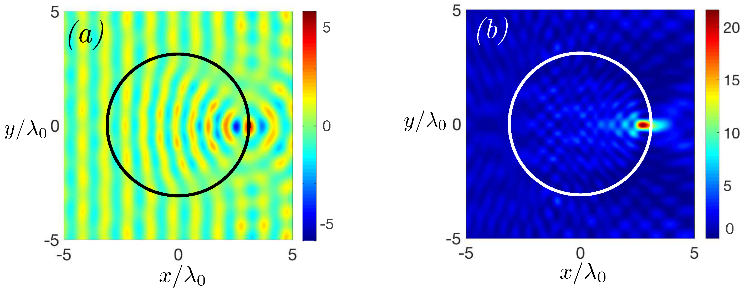
The propagation of surface water waves through the classical Luneburg lens is investigated numerically in the shallow-water regime (). Thus, the bathymetry profile is frequency-independent, and is defined by (7) with . Numerical computations are carried out, solving the SWE by a finite difference method, see Appendix B. The incident wave propagates in the forward x-direction and has unit amplitude. Figure 2a,b present the real part and the intensity (defined as ) of the calculated field, respectively. The radius of the lens is chosen to be equal to three wavelengths (, ).
Figure 2.
(Colour online) (a) Real part and (b) normalized intensity of the calculated field through a Luneburg lens in shallow water () and with (colour bars range from (blue) to 1 (red)). The incident plane wave, sent from the left, has an intensity equal to one.
Clear focusing of surface water waves is observed with the focal point of large intensity lying at the rim of the lens (the maximum of normalized intensity at the focal point is 22). The sizes of the focal point, and , defined as transverse full width at half maximum intensity, are found to be along y-axis, following the Rayleigh criterion of , and along x-axis.
This configuration (classical Luneburg lens with , in the shallow-water regime and with ) will be used in several comparisons below.
3.2. Improved Focusing Compared to Parabolic Shaped Lens
To demonstrate the enhanced focusing of the Luneburg lens compared to lenses with other profiles, calculations were made with a lens having a parabolic profile. We chose this profile because it is simple and because, as for the Luneburg lens, the focal point is located at the rim of the lens. The bathymetry profile of the parabolic lens, chosen to have the same maximum height and radius as the classical Luneburg lens, is defined as
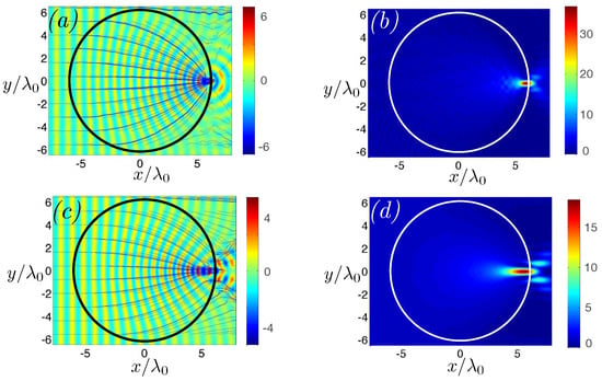
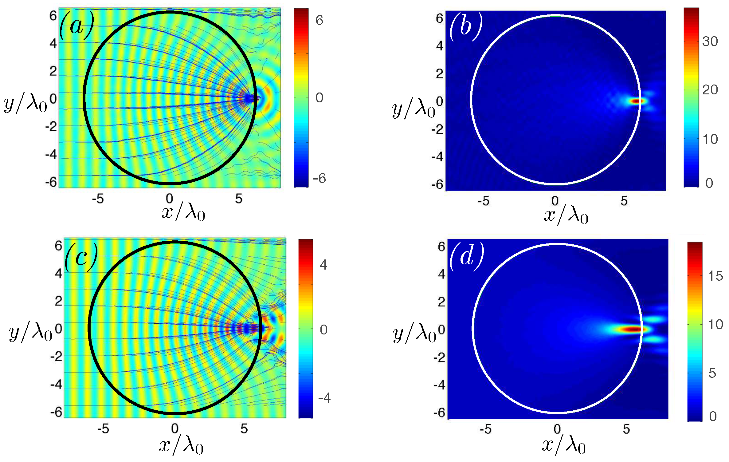
Figure 3 presents the real part and intensity of the calculated fields through the classical Luneburg lens ((a) and (b)) and the parabolic lens ((c) and (d)). Note that, compared to Section 3.1, the frequency has been increased so that .
Figure 3.
(Colour online) Real part and intensity of the field in shallow water with , through (a,b) Luneburg lens and (c,d) parabolic-shaped lens, respectively. Streamlines are represented in blue lines in the real part of the fields.
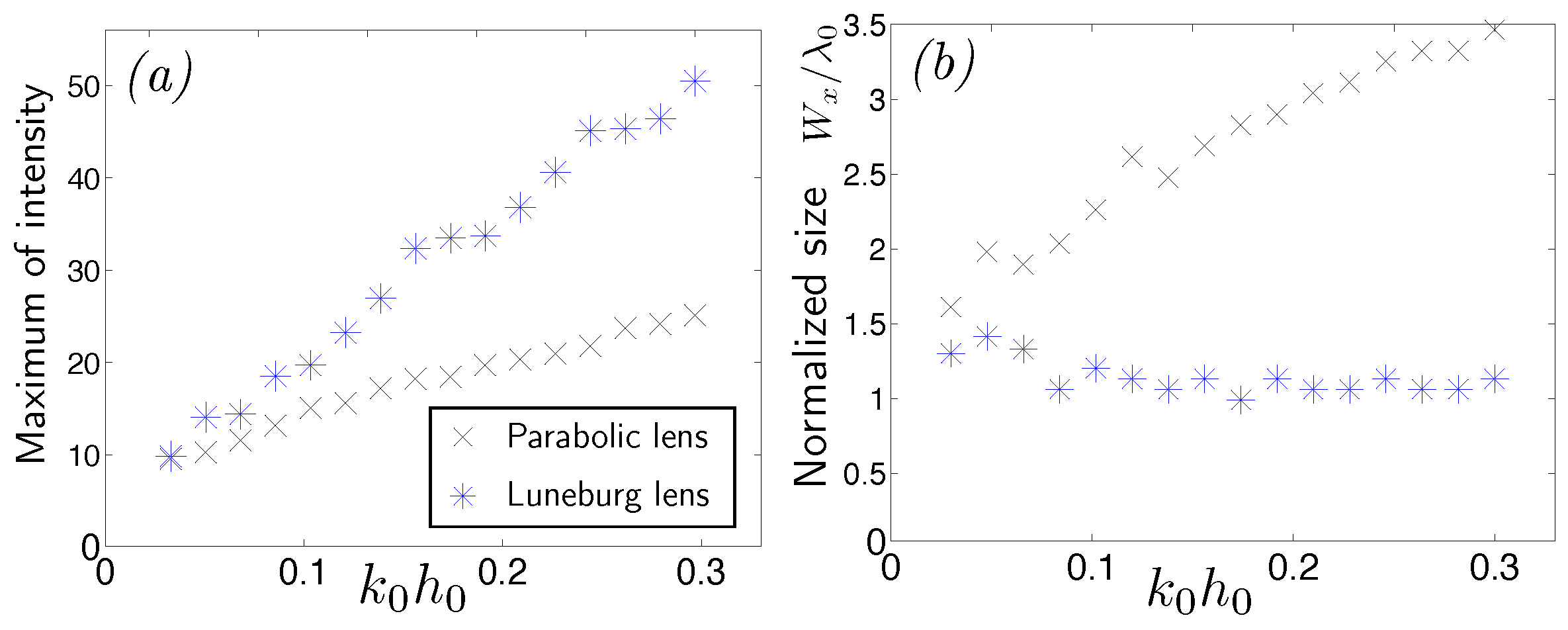
Concerning the Luneburg lens, the focusing properties are improved compared to the first reference case depicted in Figure 2, with an increase in the maximum intensity of the focal point. This result is expected: when increasing the frequency, results should become closer to the high-frequency limit of rays focusing at one point. By comparing with the focusing through the parabolic lens, Figure 3c,d, a better focusing is observed for the Luneburg lens, with smaller size and larger intensity of the focal point. The focusing of the parabolic lens suffers from a spherical aberration that occurs when the incident rays end up focusing at different points after passing the lens. The Luneburg lens, which has a refractive index that is higher at the center of the lens and gradually decreases near the edge of the lens, can eliminate the spherical aberration. An illustration of this effect can be observed by looking at the streamlines of the energy flux, which are represented as blue lines in Figure 3a,c. The rays converge better to the focal point for the Luneburg lens than for the parabolic lens, for which the rays end in a larger area. This is due to a smoother slope of the bathymetry profile of the Luneburg lens, allowing for the elimination of spherical aberration (the evolution of the maximum intensity and normalized size of the focal spot with the frequency is presented in more detail in Appendix C for both lenses). A larger increase in intensity of the focal point with frequency is revealed for the Luneburg lens compared to the parabolic lens. Its size along the x-axis is nearly equal to one wavelength for all frequencies, while that for the parabolic lens increases with frequency, reaching a value three times larger than that of the Luneburg lens.
These results demonstrate focusing of surface water waves through the classical Luneburg lens, and this focusing is enhanced compared to a parabolic mount. In order to obtain further improvement of the focusing, the modified Luneburg lens is studied in the next part. The shape of the modified Luneburg lens depends on the parameter , Equation (3), allowing the position of the focal point to be moved. The focusing properties are then analyzed as a function of this degree of freedom.
3.3. Enhanced and Tunable Focusing with the Modified Luneburg Lens
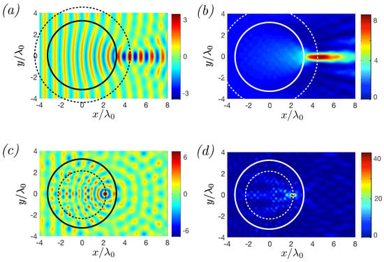
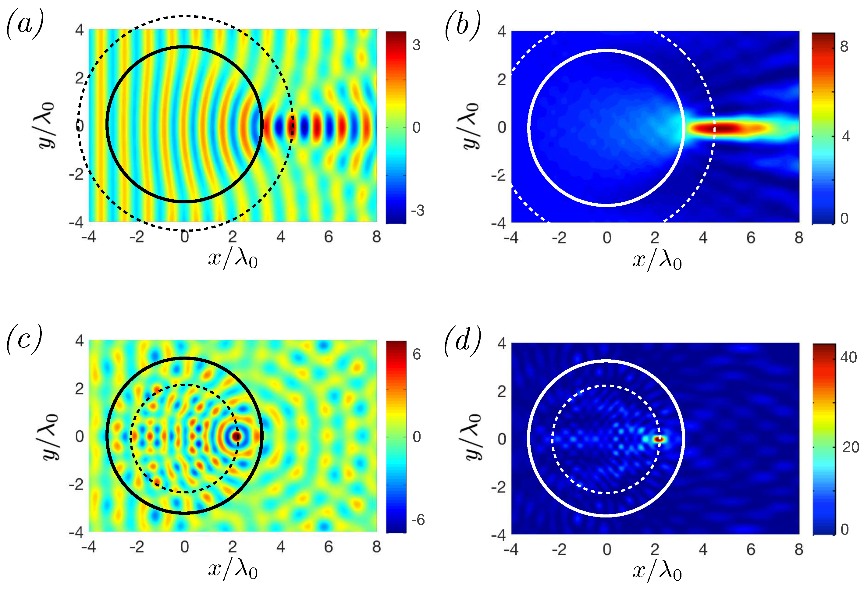
The effect of the position of the focal point is now investigated. The bathymetry profile of the modified Luneburg lens, (7), is imposed with different values of and, as for Figure 2, . Figure 4 illustrates the real part and normalized intensity fields when the focal point lies outside ((a), (b) ) and inside ((c), (d) ) the lens. The line and dotted circles represent the end of the lens and the distance , respectively. For different values of , the position of the focal point is on the dotted circle. Compared with the reference result of Figure 2 (), we can observe an increase (decrease) in focusing properties when (). In fact, when the focal point gets closer to the center of the lens, its maximum intensity increases and its size decreases.
Figure 4.
(Colour online) Real part and intensity of the field through modified Luneburg lens in shallow water with for (a,b) , and (c,d) , respectively. Line circles and dotted circles represent the end of the lens and the distance , respectively.
Note also that the field is more disturbed when decreases, which is due to an increase in the slope of the bathymetry profile when decreases. The bathymetry profile of the lens is larger when decreases, allowing the focal point to be in a shallower region. The change in water depth causes a change in wavelength. When the wave goes into a shallower region, its wavelength is reduced and then the energy is concentrated in a smaller region. So for two different values of , the focal point will be located in a shallower region for the smaller one, providing a better quality of focusing. This physical feature has also been analyzed in studies of focusing by submerged plates [15,17] or elliptical plateau [8], where it has been shown that maximum elevation is in the shallower region above the plateau or plate.
When the parameter is small, the water depth at the focal point becomes very small compared with the wavelength, so that nonlinear effects should be taken into account. A simple way to assess when nonlinearities are important is to calculate the Ursell number , where H is the wave amplitude. The nonlinear regime corresponds to [41,49,50]. For example, in the cases , and , the Ursell numbers at the focal point are , and , respectively. So, when becomes small, the Ursell number becomes very large, showing strong nonlinearities. Although the Ursell number value can be decreased by adjusting the wavelength and the wave amplitude, this paper does not consider this aspect further. However, it could be interesting to study hydrodynamic lenses using nonlinear water-wave theories [41,49,50], especially for small values of .
The MLL offers improved focusing properties when the focal point gets closer to the center of the lens. Alternatively, moving the focal point outside the lens could be useful in some applications because, for example, energy converters could be located where the bathymetry is horizontal.
The propagation of surface water waves through a Luneburg lens has been described for non-dispersive waves. It has been shown that focusing of the waves is reached at the edge of the Luneburg lens with one bathymetry profile for all frequencies belonging to the shallow-water regime. The properties of the focusing through the Luneburg lens have been shown to be better than those of a parabolic mount. Also, enhanced and tunable focusing have been shown to be possible with the MLL.
4. The Modified Luneburg Lens in the Non-Shallow-Water Regime
The propagation of waves through the MLL can be analyzed in all water-wave regimes with the Mild Slope Equation (8). We solve this equation by a finite difference method, see Appendix B, and the aim of this section is to analyze the capability of focusing of the MLL in this dispersive regime.
4.1. Evolution of the Quality of the Focusing with Frequency
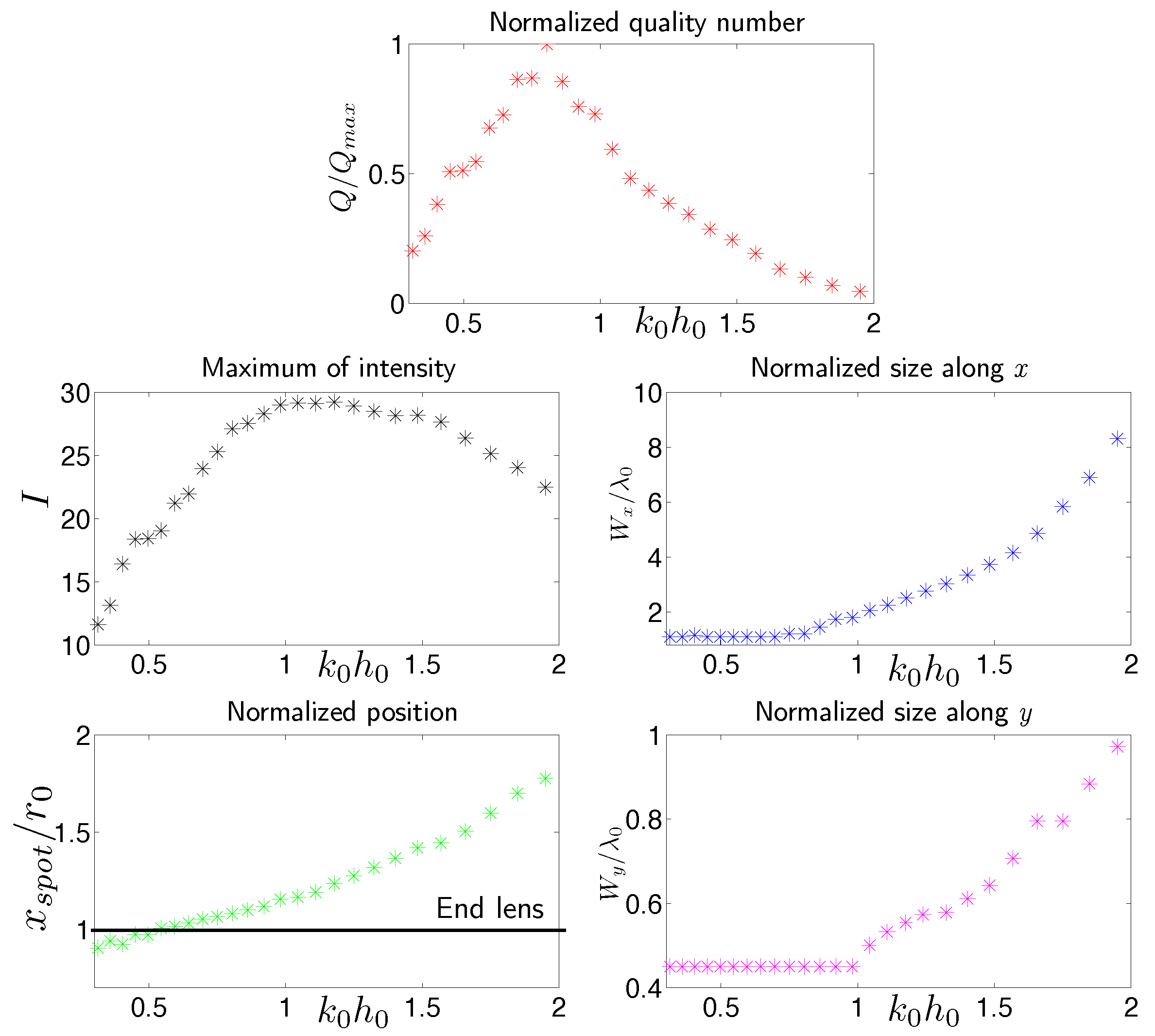
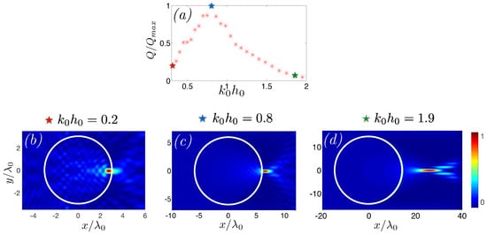
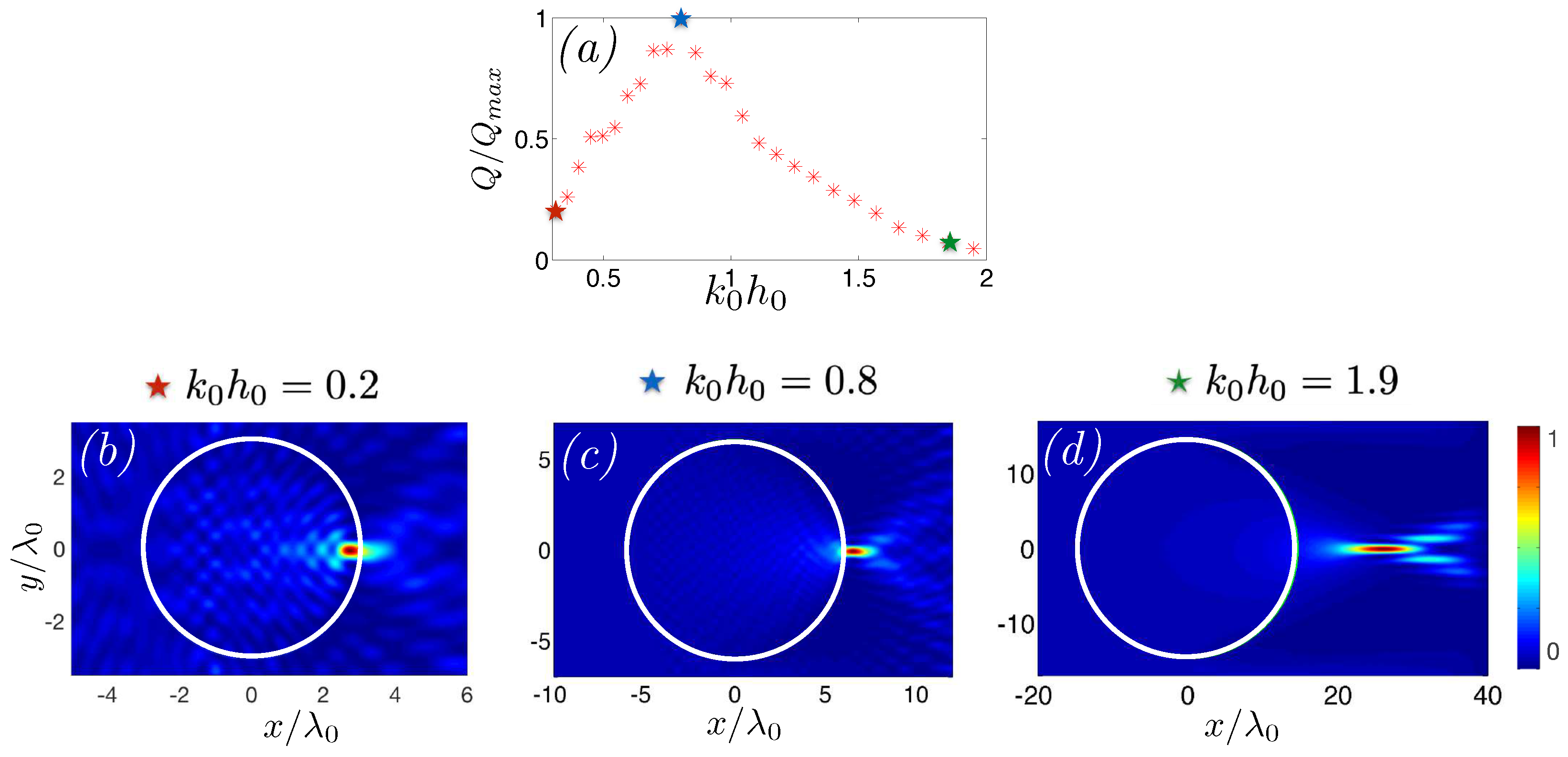
The evolution of the quality of the focusing through a fixed bathymetry is described here as a function of the frequency of the incident wave. Recall that the water depth outside the lens, , is fixed so that increasing corresponds to increasing the frequency. We start from the reference case of Figure 2 () with the bathymetry defined in shallow water (7), and then increase the frequency, thus leaving the shallow-water regime. Figure 5 presents (a) the evolution of the quality of the focusing with , and the intensity fields for (b) (reference case in shallow water), (c) and (d) . The quality of the focusing is normalized by its maximum and defined as the ratio between the maximum intensity I and the normalized sizes along y and x axes of the focal spot,
The values for the maximum intensity, normalized sizes and position of the focal point are presented in Appendix E.
Figure 5.
(Colour online) Focusing quality as a function of for a bathymetry suited for shallow-water regime and intensity fields for , and .
It is observed in Figure 5a that the quality of the focusing increases until reaching a maximum at , and then decreases. Before , the shallow-water bathymetry provides focusing at the edge of the lens, Figure 5b, and, as explained in Section 3, the increase in quality with is due to an increase in frequency (the lens contains more wavelengths). Then, starting from , the quality starts decreasing. This deterioration is due to dispersive effects (non-shallow-water regime), which leads to a shift of the focal point position to the outside of the lens, Figure 5d, and which results in a focal point with smaller intensity and larger sizes, see Appendix E. In fact, the bathymetry profile suited for shallow-water waves is no longer efficient for non-shallow-water frequencies. However, although the quality of the focusing is decreasing compared to the maximum quality, its deterioration is not important. Results are presented for a large range of values and the intensity values and sizes of the focal point are still non-negligible compared to the maximum ones. Thus, the focusing can still have good properties for a frequency range around the maximum quality.
4.2. Focusing of Dispersive Waves at a Given Frequency
It is important to notice that it is also possible to adapt the bathymetry profile to obtain optimal focusing at the edge of the lens at a desired frequency. In fact, the bathymetry profile suited at the chosen frequency can be obtained from (6). The focusing on different water-wave regimes is presented in Figure 6.
Figure 6.
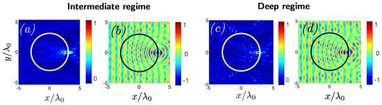
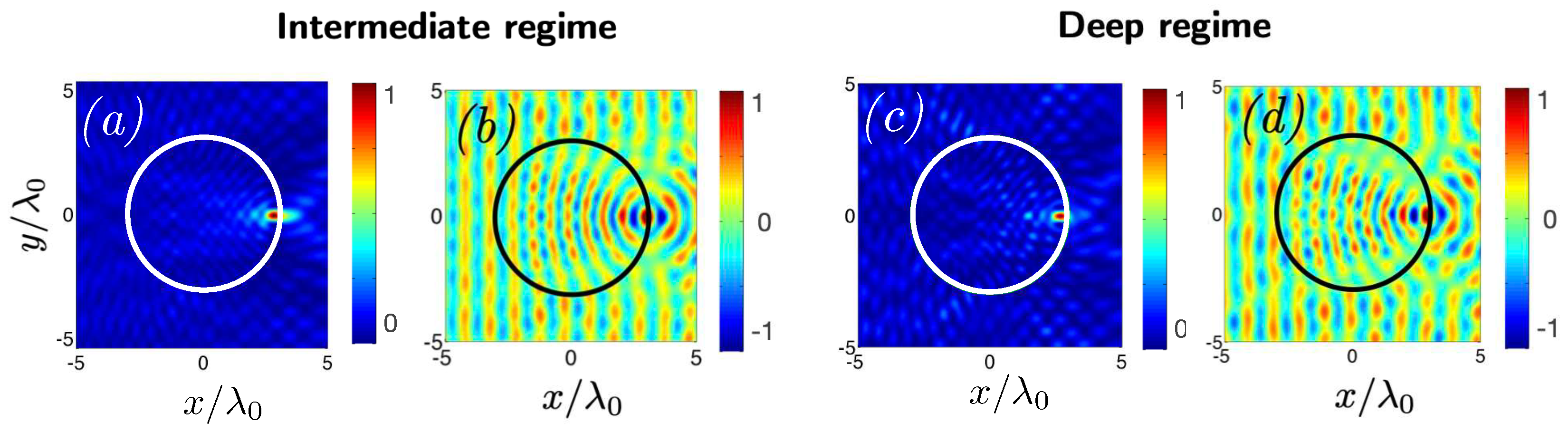
(Colour online) Intensity and real part of the calculated fields through a Luneburg lens with at (a,b) (intermediate regime) and (c,d) (deep regime) with bathymetry profile obtained for each case with (6) (colour bars are chosen to be the same).
For each regime, the bathymetry profile is given by (6). As for the reference case of Figure 2 in shallow water, results are presented for the classical Luneburg lens () and with . Figure 6a,b present the intensity and real part of the calculated fields for (intermediate regime) and (deep water regime). In all the cases, optimal focusing is obtained with the focal point lying at the rim of the lens. In the deeper water regime, the field is more disturbed, which is due to an increase in the slope of the bathymetry profile, but the lens focusing quality is still good. Note that the condition of the MSE () is valid in these calculations, with for the higher bathymetry slope (for ). Good focusing quality, as demonstrated in Section 3.3 for the shallow-water regime, is also obtained for other values of . It is thus possible to focus surface water waves with the modified Luneburg lens in all water-wave regimes.
5. Experimental Results
The experiments are made for a water depth at rest = 15 mm, a lens of radius = 200 mm and for a bathymetry profile suited for the frequency Hz. This situation corresponds to an intermediate regime with = 1.4083 (the waves are dispersive, as in Section 4). The analysis of the focusing through the Luneburg lens is made for a frequency range f = [2.5–6.5] Hz, which corresponds to = [0.66–2.53]. The lens is situated in a waveguide having the size of the lens, plane waves are generated in front of the lens and an absorbing beach is placed at the end of the waveguide to avoid undesired reflection. The bathymetry for the lens is made by use of a 3D printer with a resolution of 0.2 mm.
5.1. Linear Part of the Field
The full space-time measurements of the surface wave elevation are performed by Fourier Transform Profilometry (FTP), which has been adapted for water waves measurements ([51,52,53]). In the FTP method, a fringe pattern is projected onto the free surface and observed from a different position by the camera. The surface elevation is encoded in the fringe deformation in comparison with the original (undeformed) grating image. It is, therefore, the phase shift between the reference and deformed images that contains all information about the deformed surface. Owing to the temporal resolution, the total measured displacement field can be easily expanded in to extract the complex field that is later analyzed. The complex field corresponds to the m-th harmonic (for ) of the fundamental .
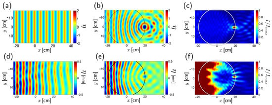
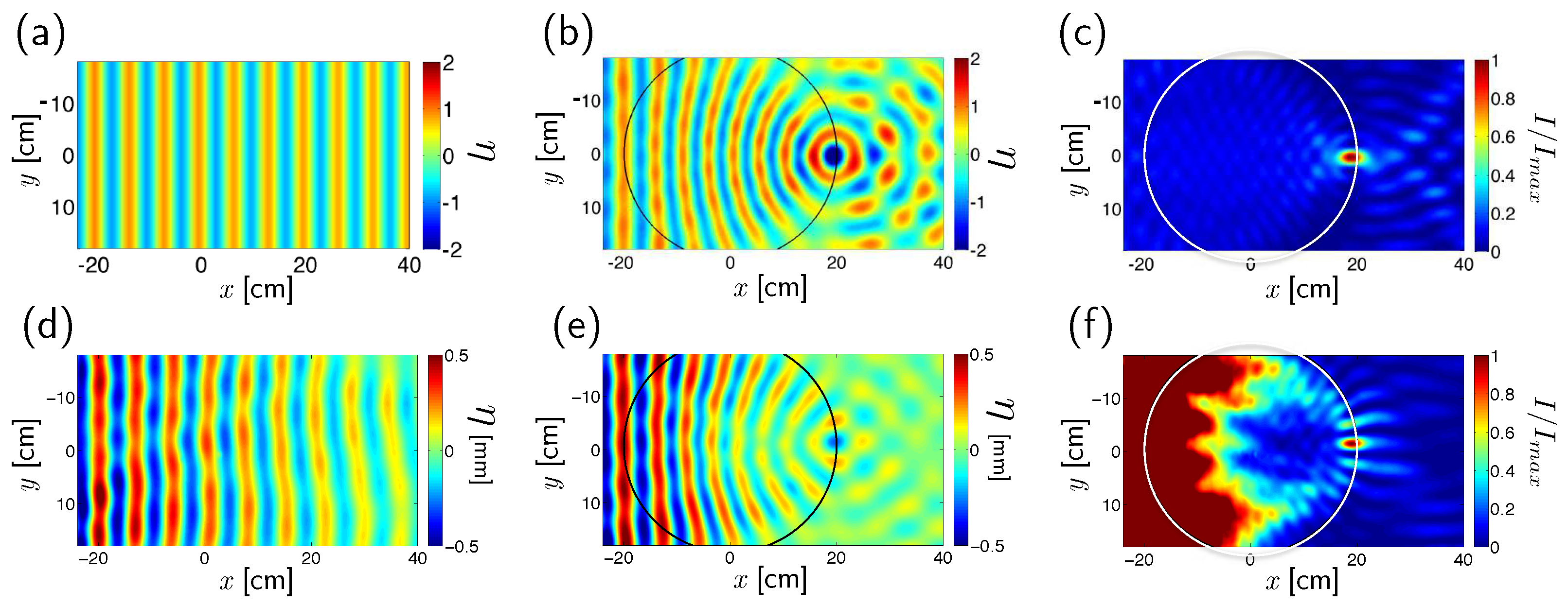
Figure 7 presents the real part and the normalized intensity field obtained by (b) (c) numerical simulations and (e) (f) experiments at the frequency Hz. The numerical simulations are performed by solving the original Mild Slope Equation by the finite difference method and by accounting for the attenuation of the waves due to viscous damping, see Appendix F. The center of the lens is at . The experimental results represent the linear component of the fields . The real part of the field without the lens is represented in Figure 7a,d for simulation and experiment, respectively. Quite an important attenuation of the waves along the propagation is observed in experiments, which is not in accordance with the simulation. This is mainly due to the experimental setup, where it is difficult to clean the surface enough to avoid the attenuation of the waves, and also due to the surface of the lens, which is not perfectly smooth. However, despite these experimental difficulties, clear focusing at the end of the lens is observed in the experiment. The properties of the focal point are very close in both cases. The axial position of the focal point is for simulation and for experiments. The sizes of the focal point along x and y axes are, respectively, and , and and , providing focusing properties below Rayleigh criterion in . Appendix G presents the evolution of the focusing with frequency.
Figure 7.
(a–c) Theoretical and (d–f) experimental results for the linear component of the field at Hz. (a,d) Real part of the elevation field without the lens, (b,e) real part of the elevation field with the lens and (c,f) intensity normalized by the maximum intensity at the focal point.
5.2. Nonlinear Focusing
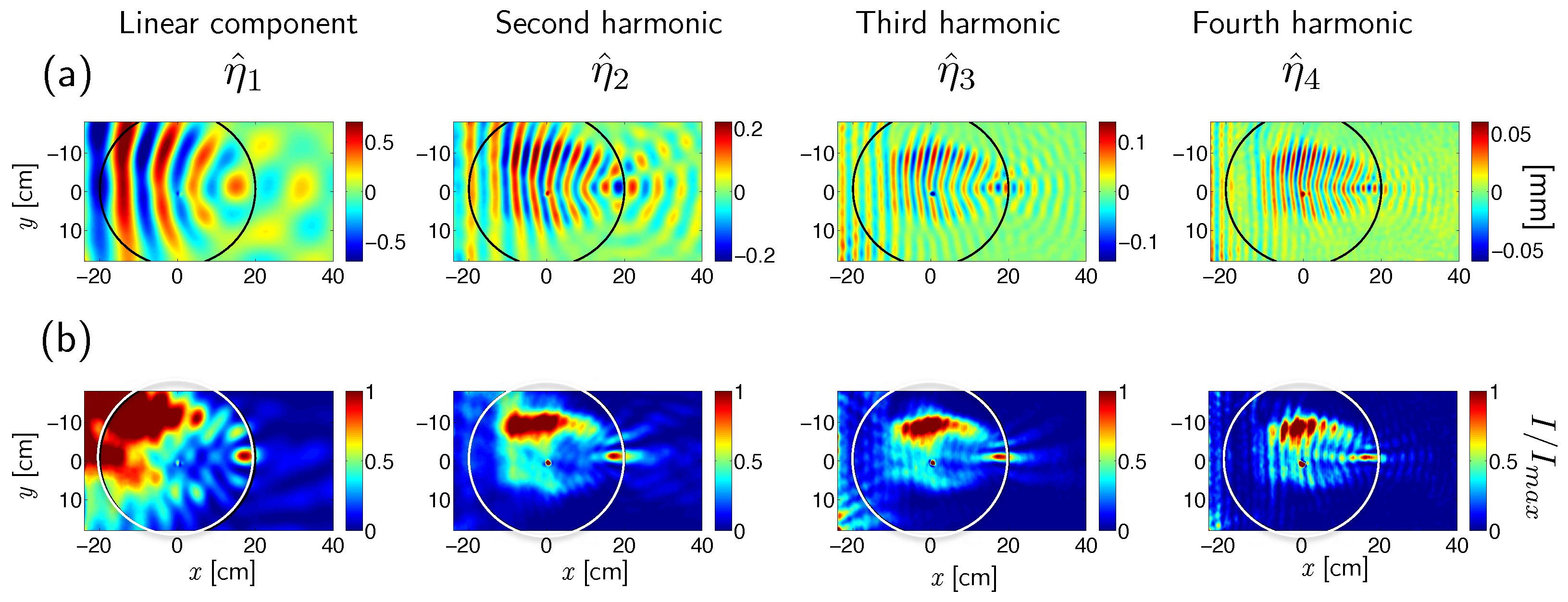
The incident wave frequency is chosen to be Hz in order to have important nonlinear components. The resulting fields after the FTP procedure are illustrated in Figure 8. The fundamental component (linear part) , the second , third and fourth harmonics of the field are presented. The harmonics are significant, with amplitude for the second, third and fourth harmonics of , and of the first harmonic, respectively. It can be seen that the amplitudes of the higher harmonics become more important inside the lens, when the water depth is smaller, as evaluated with the Ursell number. The wave deformation through the lens is clearly observed and focusing at the rim of the lens is revealed for all the components of the total field. Despite some experimental difficulties, these results have shown focusing by the Luneburg lens, and moreover, the focusing of nonlinear fields has been revealed.
Figure 8.
Experimental results at Hz. (a) Real part and (b) normalized intensity fields for the linear component of the elevation field , the second harmonic , the third harmonic and the fourth harmonic of the elevation field. is the maximum intensity at the focal point.
6. Conclusions
The focusing of surface water waves by a modified Luneburg lens has been studied for non-dispersive (shallow water) and dispersive waves. It has been shown that it is possible to build a lens free of spherical aberration, with the possibility to tune the distance between the center of the lens and the position of the focal point. It has also been revealed that the efficiency of this lens is much better than for a parabolic-shaped lens. The experimental demonstration of the Luneburg lens has confirmed its focusing effect, with observations indicating that nonlinear wave components are likewise concentrated by the lens.
Author Contributions
H.P., A.M., P.A.M., P.P. and V.P. conceived the idea, carried out the calculations and analysis, and wrote the manuscript. All authors have read and agreed to the published version of the manuscript.
Funding
H.P., A.M., P.P. and V.P. acknowledge the financial support of the Agence Nationale de la Recherche through the grant DYNAMONDE ANR-12-BS09-0027-01 and the grant CoProMM ANR-21-CE30-0046.
Institutional Review Board Statement
Not applicable.
Informed Consent Statement
Not applicable.
Data Availability Statement
The data that support the findings of this study are available from the corresponding author upon reasonable request.
Acknowledgments
The authors would like to thank Noé Jimenez for the design of Figure 1.
Conflicts of Interest
The authors declare no conflicts of interest.
Appendix A. Analytical Expression for the Water-Depth Profile
A good approximation to solve the general dispersion relation of linear water waves , due to Eckart [54], is given by
This approximation is exact in shallow and deep water regimes, and shows at most error in the intermediate regime [55]. It can be used to find an expression for the water depth as follows. We have
whence . As ,
Appendix B. Finite Difference Calculations
The SWE and MSE are solved numerically by standard finite difference methods [56]. We use a rectangular computational domain with a square grid. In all the computations, a piston boundary condition of unit amplitude is applied at the (left) entrance to the computational domain. To avoid reflection, a damping zone with a parabolic decrease in the imaginary part of the wavenumber k is imposed at the right-hand end of the domain. Neumann boundary conditions are applied at the top and bottom of the computational domain. To ensure accuracy, the grid spacing is chosen to be ten points per minimum wavelength.
In this paper, we work on a given lens geometry which is characterized by . The number of wavelengths across the lens is . Then, using
the quality of the focusing can be inspected in terms of the two parameters and N; the parameter N represents the high-frequency character of the surface waves in the horizontal plane and the parameter is linked to the sensitivity.
Appendix C. Properties of Luneburg Lens and ParabolicLens in the Shallow-Water Regime
The maximum intensity and the normalized size of the focal spot are presented for ranging from 0.06 to 0.3 in Figure A1a,b. For both lenses, the maximum intensity of the focal point increases with , which can be explained by a logical increase in the number of wavelengths in the lens when increases (A3). However, a larger increase with is observed for the Luneburg lens, following a linear slope. The intensity of the Luneburg lens is greater at and 101% greater at than those of the parabolic lens. The full width at half maximum of intensity of the focal point along x-axis is nearly equal to one wavelength for all for the Luneburg lens, whereas the width increases with for the parabolic shape, Figure A1b, reaching a value that is three times larger than that of the Luneburg lens at .
Figure A1.
(Colour online) (a) Maximum of intensity and (b) full width at half maximum of the intensity along -axis of the focal point for Luneburg lens (blue asterisks) and for parabolic shaped lens (black crosses). Incident wave has intensity 1.
Appendix D. Maximum of Intensity for Modified Luneburg Lens as a Function of αf and k0h0
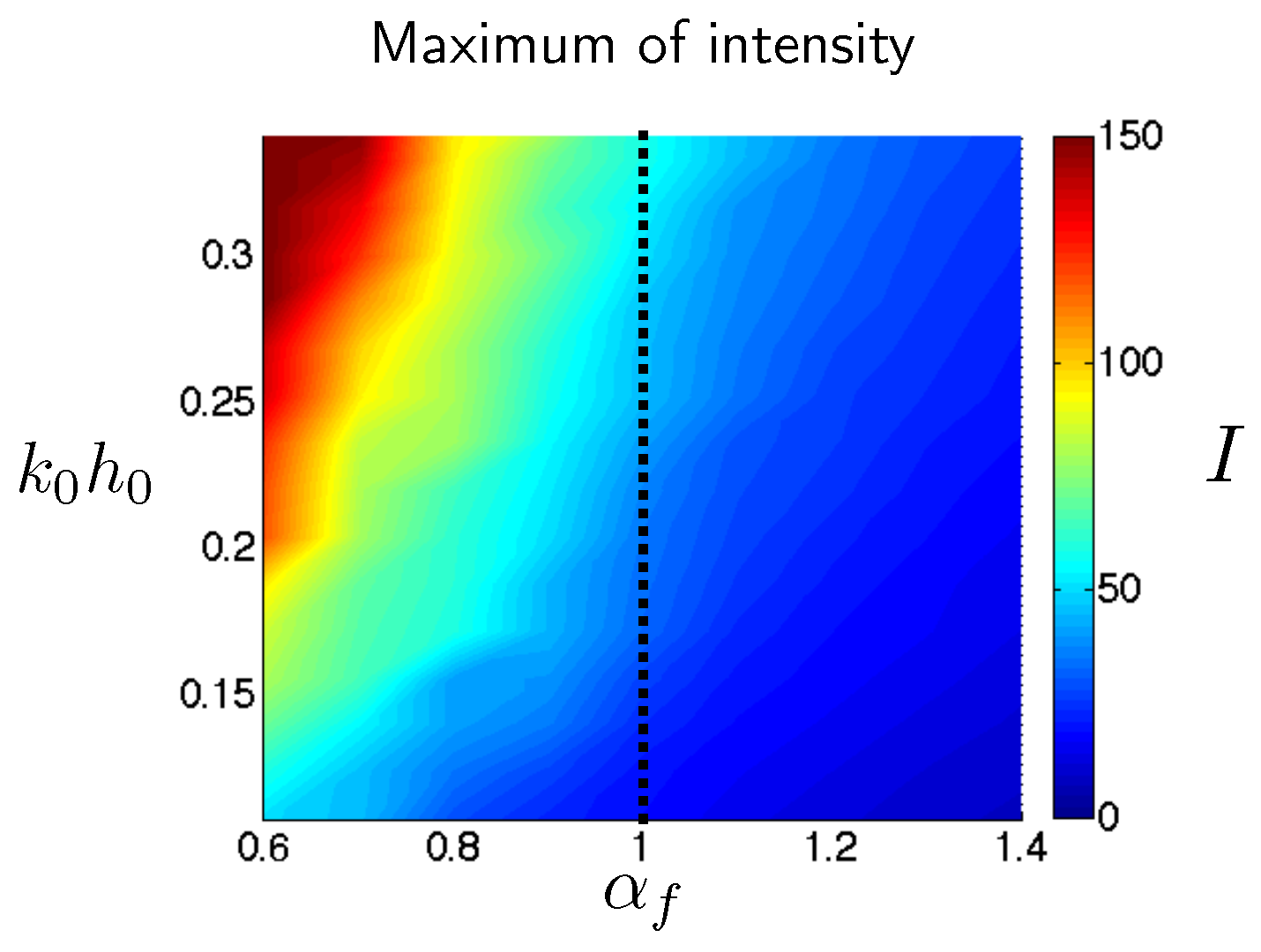
Figure A2 presents the maximum intensity of the focal point for more values of and for ranging from 0 to . Computations are performed with six wavelengths across the lens at . For a given , the intensity of the focal point increases when increases. Moreover, for all , enhanced focusing is observed when decreases.
Figure A2.
(Colour online) Maximum intensity of the focal point as a function of with ranging from 0 to 0.35.
Appendix E. Evolution of Properties of the Focusing with k0h0 When the Bathymetry Is Fixed
Figure A3 presents the evolution of the focusing properties with with the bathymetry profile suited for shallow-water waves. The maximum of intensity, normalized position and normalized sizes of the focal point are depicted as functions of .
Figure A3.
(Colour online) Properties of the focusing as a function of with shallow-water profile.
Appendix F. Attenuation and Surface Tension Effects
In this section, dissipation due to viscous damping is included in the model. For waves propagating in a channel, losses due to viscous damping [57] can be taken into account by adding an imaginary part of the wavenumber k in the form , where is the real part of the wavenumber (solution of the dispersion relation (4)),
b is the width of the channel and is the kinematic viscosity. The width of the channel is chosen to be and the viscosity as that of water.
As the dissipation depends on the actual size of the setup, results for three different sizes are given. Figure A4 presents results for propagation through the classical Luneburg lens (the reference case of Figure 2), taking dissipation into account, for three values of the radius of the lens: small scale m, intermediate scale m and large scale m.
Figure A4.
(Colour online) Real part of the fields for Luneburg lens accounting for viscous damping and with . (a) Small scale ( m). (b) Intermediate scale ( m). (c) Large scale ( m). (d) Intensity along the -axis at the maximum of the focal point (at ).
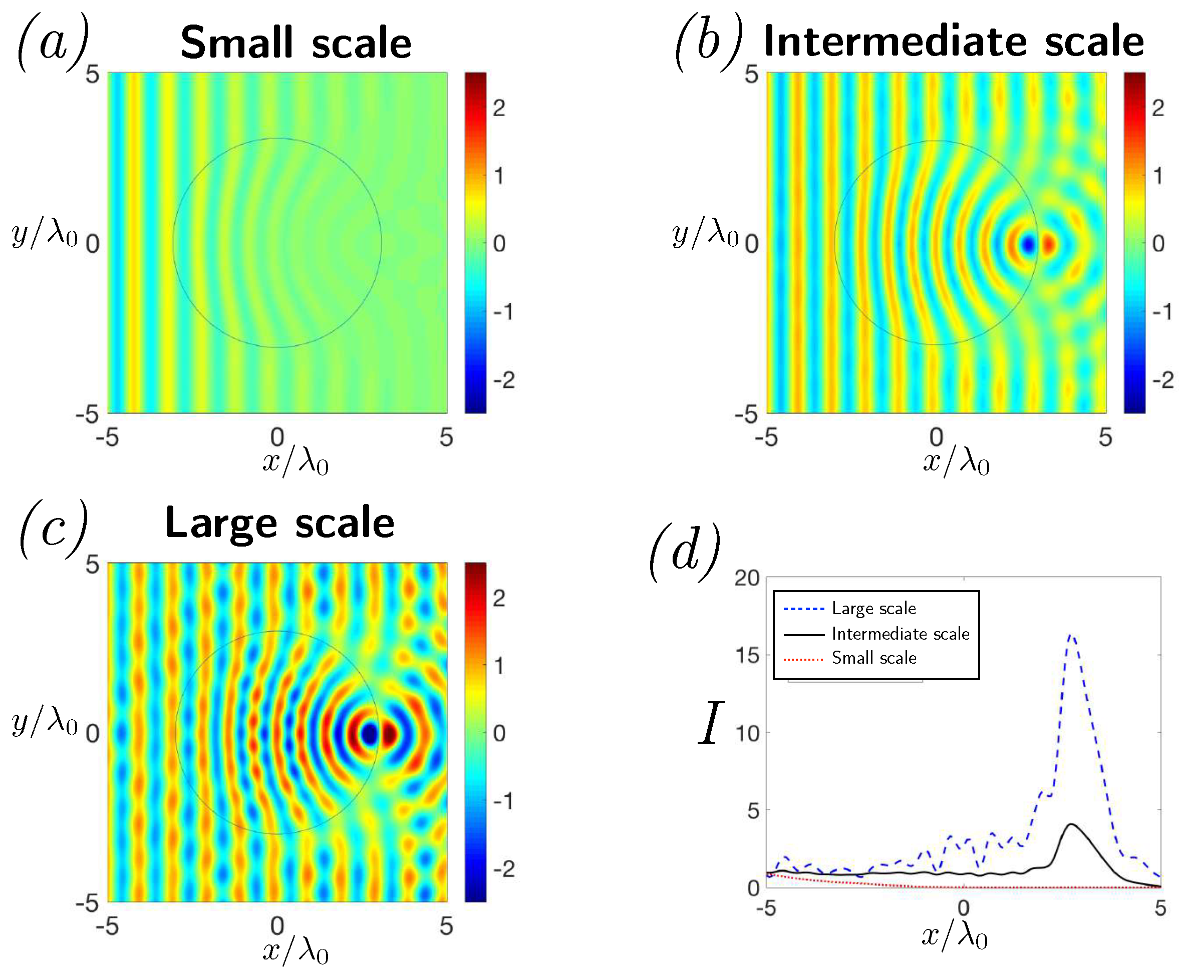
For the sake of comparison, the same colour bar is used in Figure A4a–c. Figure A4d presents the intensity along a line passing through the maximum of the focal point (at ) and along the -axis.
For small scale, dissipation effects have a strong influence on the focusing, because of a strong and quick attenuation of the waves along the propagation direction. However, for intermediate and large scales, focusing is revealed with an increasing of the maximum of intensity of the focal point when the setup gets larger, Figure A4d. Thus, even if it may be difficult to highlight the focusing in a small laboratory setup for example, the focusing by the Luneburg lens will be efficient in ocean configurations. Note also that it is possible to reduce the dissipation effects by adjusting other parameters such as or the frequency. The important point will be to correctly account for dissipation to adapt to the physical setup of interest. Note that the effects of attenuation due to viscous damping are more important in shallow water and will be reduced when increasing .
Since water has significant surface tension, its effects on the focusing should be estimated. The wave dispersion accounting for surface tension is given by
with the surface tension at 20 °C and the water density .
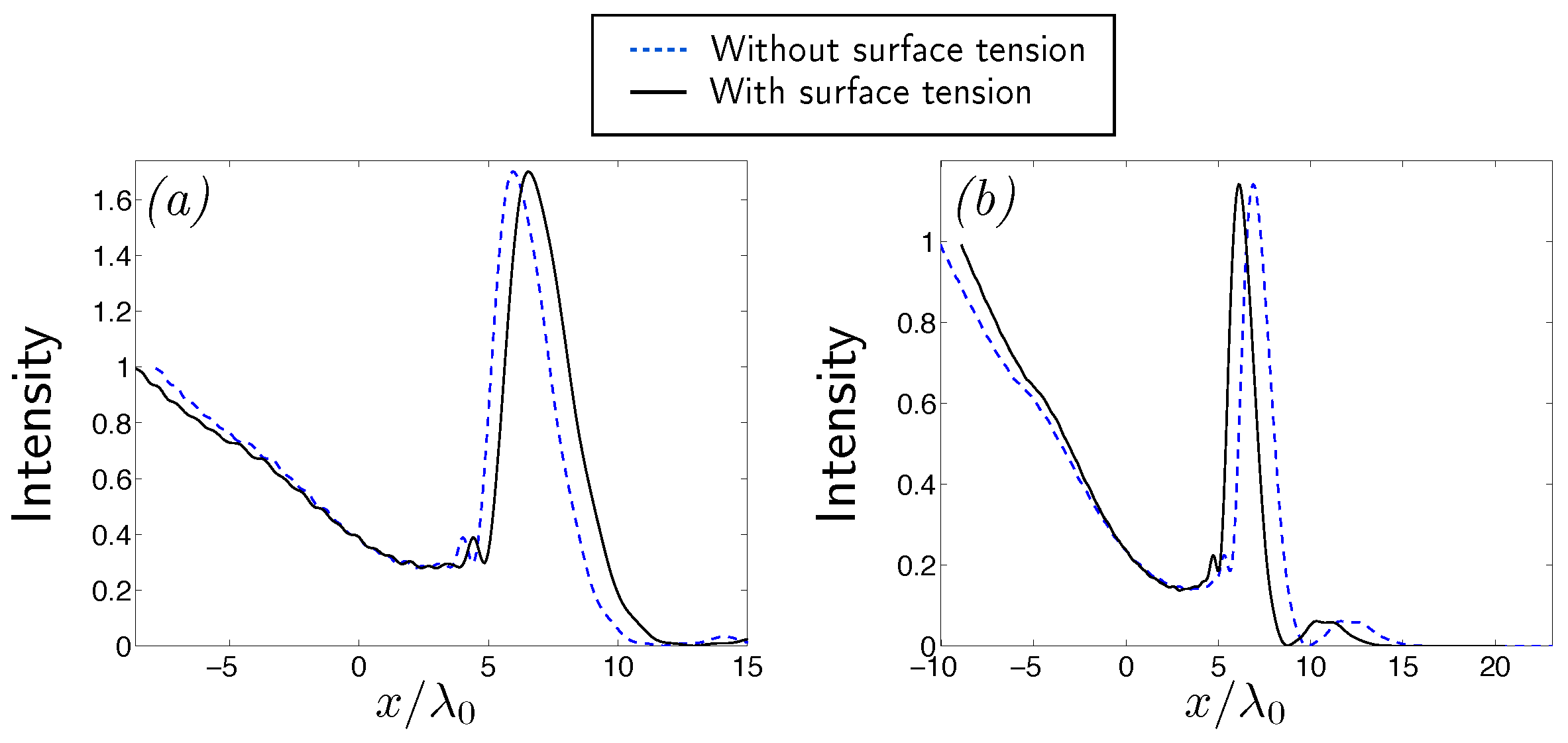
In the case of Figure A4, the new term in the dispersion relation (A5) induces a wavenumber being smaller than the one without surface tension. Figure A5 shows the intensity of the field along the -axis at through the classical Luneburg lens for , with (black continuous line) and without (blue dotted line) surface tension. Dissipation is taken into account. The number of wavelengths across the lens are chosen to be in Figure A5a and in Figure A5b. The consideration of surface tension induces small differences. A shift of the position of the focal point of less than is observed, and its intensity and size are the same. As illustrated in Figure A5b with , when increasing N the wavelength decreases, and surface tension has more effect, but with still negligible effect on the focusing. Logically, the effects of surface tension will decrease when increasing the radius of the lens. In fact, in the case of intermediate and large scales ( m, m), the difference between wavenumber value with and without surface tension is less than , which has no effect on the focusing.
Figure A5.
(Colour online) Intensity field along the -axis at , when in small scale ( m and mm), when , with accounting for surface tension (black continuous line) and without accounting for it (blue dotted line). (a) and (b) , where N is the number of wavelengths across the lens.
Appendix G. Experimental Results for Several Frequencies
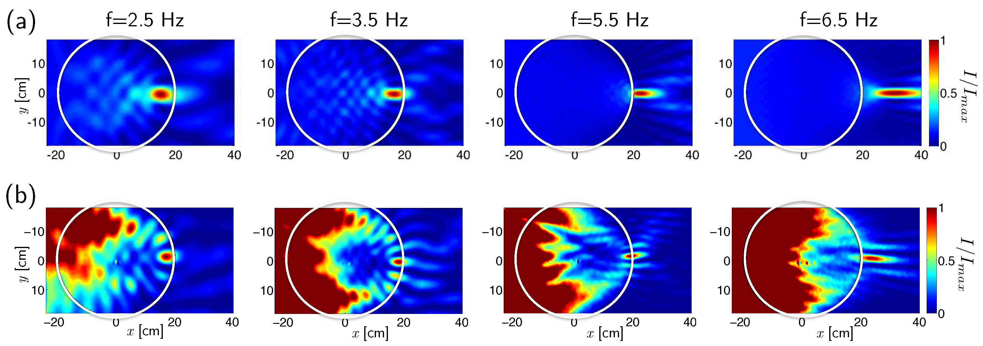
The experimental results are presented for the frequencies f = [2.5–6.5] Hz. Figure A6a,b shows the simulated and experimental normalized intensity of the linear fields for different frequencies. Focusing is clearly observed for all the frequencies, with, despite the attenuation effect in experiment, strong similarities between simulations and experiments. As predicted by theory, the focal point position is shifted the outside of the lens when the frequency increases. Just a little shift of position between experiments and simulations is observed.
Figure A6.
Normalized intensity of the linear component of the elevation field at different frequencies. (a) Simulations. (b) Experiments.
References
- Ito, Y.; Tanimoto, K. A method of numerical analysis of wave propagation—Application to wave diffraction and refraction. In Proceedings of the 13th Coastal Engineering Conference, Vancouver, BC, Canada, 10–14 July 1972; pp. 503–522. [Google Scholar]
- Vincent, C.L.; Briggs, M.J. Refraction—Diffraction of irregular waves over a mound. J. Waterw. Port Coast. Ocean Eng. 1989, 115, 269–284. [Google Scholar] [CrossRef] [Scilit]
- Berkhoff, J.C.W.; Booy, N.; Radder, A.C. Verification of numerical wave propagation models for simple harmonic linear water waves. Coast. Eng. 1982, 6, 255–279. [Google Scholar] [CrossRef] [Scilit]
- Mei, C.C. The Applied Dynamics of Ocean Surface Waves; John Wiley and Sons: New York, NY, USA, 1983. [Google Scholar]
- Murashige, S.; Kinoshita, T. An ideal ocean wave focusing lens and its shape. Appl. Ocean Res. 1992, 14, 275–290. [Google Scholar] [CrossRef] [Scilit]
- McCormick, M.E. Ocean Wave Energy Conversion; Wiley: Hoboken, NJ, USA, 1981. [Google Scholar]
- Brooks, J. Wave Energy Conversion; Elsevier: Amsterdam, The Netherlands, 2003. [Google Scholar]
- Griffiths, L.S.; Porter, R. Focusing of surface waves by variable bathymetry. Appl. Ocean Res. 2012, 34, 150–163. [Google Scholar] [CrossRef] [Scilit]
- Arthur, R.S. Refraction of water waves by islands and shoals with circular bottom-contours. Am. Geophys. Union 1946, 27, 168–177. [Google Scholar]
- Kriegsmann, G.A. An illustrative model describing the refraction of long water waves by a circular island. J. Phys. Oceanogr. 1979, 9, 607–611. [Google Scholar] [CrossRef] [Scilit]
- Mehlum, E. A circular cylinder in water waves. Appl. Ocean Res. 1980, 2, 171–177. [Google Scholar] [CrossRef] [Scilit]
- Stamnes, J.J.; Løvhaugen, O.; Spjelkavik, B.; Mei, C.C.; Lo, E.; Yue, D.K.P. Nonlinear focusing of surface waves by a lens—Theory and experiment. J. Fluid Mech. 1983, 135, 71–94. [Google Scholar] [CrossRef] [Scilit]
- Stamnes, J.J. Waves in Focal Regions: Propagation, Diffraction and Focusing of Light, Sound and Water Waves; Taylor & Francis: Abingdon, UK, 1986. [Google Scholar]
- Kudo, K.; Tsuzuku, T.; Iwai, K.; Akiyama, Y. Wave focusing by a submerged plate. In Proceedings of the OCEANS ’88. A Partnership of Marine Interests. Proceedings, Baltimore, MD, USA, 31 October–2 November 1988; pp. 1061–1066. [Google Scholar]
- Teigen, P. On wave amplification over submerged lenses. In Proceedings of the 23rd International Workshop on Water Waves and Floating Bodies, Jeju, Republic of Korea, 13–16 April 2008. [Google Scholar]
- Choi, J.; Lim, C.H.; Lee, J.I.; Yoon, S.B. Evolution of waves and currents over a submerged laboratory shoal. Coast. Eng. 2009, 56, 297–312. [Google Scholar] [CrossRef] [Scilit]
- Newman, J.N. Amplification of waves by submerged plates. In Proceedings of the 30th International Workshop on Water Waves and Floating Bodies, Bristol, UK, 12–15 April 2015. [Google Scholar]
- Ricard, G.; Novkoski, F.; Falcon, E. Effects of nonlinearity on Anderson localization of surface gravity waves. Nat. Commun. 2024, 15, 5726. [Google Scholar] [CrossRef] [Scilit]
- Hu, X.; Chan, C.T. Refraction of water waves by periodic cylinder arrays. Phys. Rev. Lett. 2005, 95, 154501. [Google Scholar] [CrossRef] [Scilit]
- Yang, J.; Tang, Y.F.; Ouyang, C.F.; Liu, X.H.; Hu, X.H.; Zi, J. Observation of the focusing of liquid surface waves. Appl. Phys. Lett. 2009, 95, 094106. [Google Scholar] [CrossRef] [Scilit]
- Wang, Z.; Zhang, P.; Nie, X.; Zhang, Y. Focusing of liquid surface waves by gradient index lens. Europhys. Lett. 2014, 108, 24003. [Google Scholar] [CrossRef] [Scilit]
- Hu, X.; Chan, C.T.; Ho, K.M.; Zi, J. Negative effective gravity in water waves by periodic resonator arrays. Phys. Rev. Lett. 2011, 106, 174501. [Google Scholar] [CrossRef] [Scilit] [PubMed]
- Hu, X.; Yang, J.; Zi, J.; Chan, C.T.; Ho, K.M. Experimental observation of negative effective gravity in water waves. Sci. Rep. 2013, 3, 1916. [Google Scholar] [CrossRef] [Scilit] [PubMed]
- Bobinski, T.; Eddi, A.; Petitjeans, P.; Maurel, A.; Pagneux, V. Experimental demonstration of epsilon-near-zero water waves focusing. Appl. Phys. Lett. 2015, 107, 014101. [Google Scholar] [CrossRef] [Scilit]
- Zhang, C.; Chan, C.T.; Hu, X. Broadband focusing and collimation of water waves by zero refractive index. Sci. Rep. 2014, 4, 6979. [Google Scholar] [CrossRef] [Scilit]
- Berraquero, C.P.; Maurel, A.; Petitjeans, P.; Pagneux, V. Experimental realization of a water-wave metamaterial shifter. Phys. Rev. E 2013, 88, 051002. [Google Scholar] [CrossRef] [Scilit]
- Kinsler, P.; Tan, J.; Thio, T.C.Y.; Trant, C.; Kandapper, N. Maxwell’s fishpond. Eur. J. Phys. 2012, 33, 1737–1750. [Google Scholar] [CrossRef] [Scilit]
- Wang, Z.; Zhang, P.; Nie, X.; Zhang, Y. Manipulating water wave propagation via gradient index media. Sci. Rep. 2015, 5, 16846. [Google Scholar] [CrossRef] [Scilit]
- Luneburg, R.K. Mathematical Theory of Optics; University of California Press: Oakland, CA, USA, 1964. [Google Scholar]
- Leonhardt, U.; Philbin, T. Geometry and Light: The Science of Invisibility; Courier Corporation: Dover, DE, USA, 2010. [Google Scholar]
- Gutman, A.S. Modified Luneberg lens. J. Appl. Phys. 1954, 25, 855–859. [Google Scholar] [CrossRef] [Scilit]
- Cheng, Q.; Ma, H.F.; Cui, T.J. Broadband planar Luneburg lens based on complementary metamaterials. Appl. Phys. Lett. 2009, 95, 181901. [Google Scholar] [CrossRef] [Scilit]
- Tyc, T.; Herzánová, L.; Šarbort, M.; Bering, K. Absolute instruments and perfect imaging in geometrical optics. New J. Phys. 2011, 13, 115004. [Google Scholar] [CrossRef] [Scilit]
- Zentgraf, T.; Liu, Y.; Mikkelsen, M.H.; Valentine, J.; Zhang, X. Plasmonic Luneburg and Eaton lenses. Nat. Nanotech. 2011, 6, 151–155. [Google Scholar] [CrossRef] [Scilit] [PubMed]
- Di Falco, A.; Kehr, S.C.; Leonhardt, U. Luneburg lens in silicon photonics. Opt. Express 2011, 19, 5156–5162. [Google Scholar] [CrossRef] [Scilit] [PubMed]
- Climente, A.; Torrent, D.; Sánchez-Dehesa, J. Omnidirectional broadband insulating device for flexural waves in thin plates. J. Appl. Phys. 2013, 114, 214903. [Google Scholar] [CrossRef] [Scilit]
- Climente, A.; Torrent, D.; Sánchez-Dehesa, J. Gradient index lenses for flexural waves based on thickness variations. Appl. Phys. Lett. 2014, 105, 064101. [Google Scholar] [CrossRef] [Scilit]
- Lefebvre, G.; Dubois, M.; Beauvais, R.; Achaoui, Y.; Ing, R.K.; Guenneau, S.; Sebbah, P. Experiments on Maxwell’s fish-eye dynamics in elastic plates. Appl. Phys. Lett. 2015, 106, 024101. [Google Scholar] [CrossRef] [Scilit]
- Jin, Y.; Torrent, D.; Pennec, Y.; Pan, Y.; Djafari-Rouhani, B. Gradient index devices for the full control of elastic waves in plates. Sci. Rep. 2016, 6, 24437. [Google Scholar] [CrossRef] [Scilit]
- Berkhoff, J.C.W. Computation of combined refraction-diffraction. In Proceedings of the 13th Coastal Engineering Conference, Vancouver, BC, Canada, 10–14 July 1972; pp. 471–490. [Google Scholar]
- Mei, C.C.; Stiassnie, M.; Yue, D.K.P. Theory and Applications of Ocean Surface Waves: Nonlinear Aspects; World Scientific: Singapore, 2005. [Google Scholar]
- Porter, D.; Staziker, D.J. Extensions of the mild-slope equation. J. Fluid Mech. 1995, 300, 367–382. [Google Scholar] [CrossRef] [Scilit]
- Porter, D. The mild-slope equations. J. Fluid Mech. 2003, 494, 51–63. [Google Scholar] [CrossRef] [Scilit]
- Lee, C.; Yoon, S.B. Effect of higher-order bottom variation terms on the refraction of water waves in the extended mild-slope equations. Ocean Eng. 2004, 31, 865–882. [Google Scholar] [CrossRef] [Scilit]
- Kim, J.W.; Bai, K.J. A new complementary mild-slope equation. J. Fluid Mech. 2004, 511, 25–40. [Google Scholar] [CrossRef] [Scilit]
- Hsu, T.W.; Lin, T.Y.; Wen, C.C.; Ou, S.H. A complementary mild-slope equation derived using higher-order depth function for waves obliquely propagating on sloping bottom. Phys. Fluids 2006, 18, 087106. [Google Scholar] [CrossRef] [Scilit]
- Liu, Y.Z.; Shi, J.Z. A theoretical formulation for wave propagations over uneven bottom. Ocean Eng. 2008, 35, 426–432. [Google Scholar] [CrossRef] [Scilit]
- Inan, A.; Balas, L. Numerical modeling of extended mild slope equation with modified Mac Cormack method. WSEAS Trans. Fluid Mech. 2009, 4, 14–23. [Google Scholar]
- Dingemans, M.W. Water Wave Propagation over Uneven Bottoms; World Scientific: Singapore, 1997. [Google Scholar]
- Dean, R.G.; Dalrymple, R.A. Water Wave Mechanics for Engineers and Scientists; World Scientific: Singapore, 1991. [Google Scholar]
- Cobelli, P.; Maurel, A.; Pagneux, V.; Petitjeans, P. Global measurement of water waves by Fourier transform profilometry. Exp. Fluids 2009, 46, 1037. [Google Scholar] [CrossRef] [Scilit]
- Maurel, A.; Cobelli, P.; Pagneux, V.; Petitjeans, P. Experimental and theoretical inspection of the phase-to-height relation in Fourier transform profilometry. Appl. Opt. 2009, 48, 380. [Google Scholar] [CrossRef] [Scilit]
- Przadka, A.; Cabane, B.; Pagneux, V.; Maurel, A.; Petitjeans, P. Fourier transform profilometry for water waves: How to achieve clean water attenuation with diffusive reflection at the water surface? Exp. Fluids 2012, 52, 519. [Google Scholar] [CrossRef] [Scilit]
- Eckart, C. The propagation of gravity waves from deep to shallow water. In Proceedings of the Gravity Waves. National Bureau Standards, Circular 521; U.S. Government Printing Office: Washington, DC, USA, 1952; pp. 165–173. [Google Scholar]
- Fenton, J.D.; McKee, W.D. On calculating the lengths of water waves. Coast. Eng. 1990, 14, 499–513. [Google Scholar] [CrossRef] [Scilit]
- Ames, W.F. Numerical Methods for Partial Differential Equations, 3rd ed.; Academic Press: Cambridge, MA, USA, 1992. [Google Scholar]
- Hunt, J.N. Viscous damping of waves over an inclined bed in a channel of finite width. La Houille Blanche 1952, 7, 836–842. [Google Scholar] [CrossRef] [Scilit]
Disclaimer/Publisher’s Note: The statements, opinions and data contained in all publications are solely those of the individual author(s) and contributor(s) and not of MDPI and/or the editor(s). MDPI and/or the editor(s) disclaim responsibility for any injury to people or property resulting from any ideas, methods, instructions or products referred to in the content. |
© 2026 by the authors. Licensee MDPI, Basel, Switzerland. This article is an open access article distributed under the terms and conditions of the Creative Commons Attribution (CC BY) license.