


Abstract
This data descriptor presents a dataset comprising crop and soil parameters measured in winter wheat fields near the town of Knezha, Bulgaria. The data were collected as part of a project evaluating the potential of vegetation indices derived from Sentinel-2 satellite imagery to predict biophysical and biochemical crop parameters. The core dataset consists of measurements obtained from 20 m × 20 m field plots and includes a broad range of parameters: leaf area index, fraction of absorbed photosynthetically active radiation, vegetation cover fraction, chlorophyll content, above-ground biomass, plant nitrogen content, biological yield, surface soil moisture, spectral reflectance, plant density, crop height, visual assessments of disease or pest damage, and data on weed occurrence. The dataset is complemented by unmanned aerial vehicle imagery, crop calendars, and field management information. The main soil types in the study area were characterized through soil profiles, while meteorological data were obtained from an automated weather station. The data were collected during the 2016–2017 and 2017–2018 agricultural seasons. The dataset is freely available for download and serves as a valuable resource for researchers in remote sensing—particularly for validating satellite-derived products—as well as for specialists involved in winter wheat monitoring, modeling, and agronomic studies.
Dataset: In situ and UAV dataset with crop and soil parameters obtained from winter wheat fields. https://doi.org/10.5281/zenodo.17475742.
Dataset License: Data are available under the terms of the Creative Commons Attribution 4.0 International public license.
1. Summary
With the launch of the first Sentinel-2 satellite in 2015, the capabilities for operational, large-scale, and timely satellite monitoring of crops were significantly enhanced. The Sentinel-2 constellation, which currently includes three satellites in orbit, provides images in multiple spectral bands, well-suited to capturing vegetation reflectance patterns and offering high spatial and temporal resolution. This technological advancement has driven the development of new protocols and methods for deriving crop-state information from satellite observations.
One such effort was the TS2AgroBg project (“Testing Sentinel-2 vegetation indices for the assessment of the state of winter crops in Bulgaria”). The project aimed to calibrate and validate empirical models to predict and map key crop parameters, such as leaf area index, biomass, and chlorophyll content, using Sentinel-2 vegetation indices. Another major objective was to provide a methodology for the integral assessment of crop status based on a combination of such parameters.
The development and validation of these models required extensive ground-truth data for the modeled crop parameters, necessitating dedicated field campaigns. A series of such field campaigns was conducted over two agricultural seasons, focusing on winter wheat (Triticum aestivum L.), the predominant crop in the country. The campaigns took place in agricultural fields where various crop and soil parameters were measured in 20 m × 20 m Elementary Sampling Units (ESUs). The goal was to comprehensively characterize the crop’s condition by collecting biophysical, biochemical, biometric, phenological and surface soil moisture data. Measurements were performed at several key stages of crop development to capture temporal variations throughout the growing season.
Auxiliary data were also collected to support the analysis and interpretation of results, including: (1) soil profile data from four locations within the study fields; (2) crop calendar and management information; (3) Unmanned Aerial Vehicle (UAV) multispectral imagery; and (4) meteorological data from an automated weather station installed in the study area.
The dataset resulting from these field campaigns has been published and is freely available to the research community. It can serve not only for the development and validation of remote sensing–based crop monitoring algorithms but also for a range of other applications requiring in situ data on winter wheat. This data descriptor provides a detailed description of the data collection methods and the structure and content of the resulting dataset.
2. Data Description
The dataset includes nine tab-delimited text files containing various in situ parameters, such as crop biophysical and biochemical data, spectral data, and phenological data. Each of them is given a descriptive file name to facilitate its use. Each file is accompanied by a metadata text file with the same name, ending with “_info”, that describes the columns and units of measurement. In addition, three ESRI Shapefiles are provided as zip archives, each containing the locations of agricultural fields, ESUs, and soil profiles. Finally, the UAV mosaics are provided in 17 zip archives, each containing four spectral bands as separate .tif files. A full description of the files is provided below:
- “ESU_Biophysical_and_biochemical_crop_data.txt”—a tab-delimited text file containing Leaf Area Index (LAI), fraction of Intercepted Photosynthetically Active Radiation (fIPAR), Fraction of Absorbed Photosynthetically Active Radiation (fAPAR), Vegetation cover fraction (fCover), Chlorophyll content (CC), Above-ground biomass (AGB), Plant nitrogen content, and biological yield data per ESU.
- “ESU_Biophysical_and_biochemical_crop_data_info.txt”—a tab-delimited text file containing a column description for the file “Biophysical_and_biochemical_crop_data.txt”.
- “ESU_Field_spectral_data.txt”—a tab-delimited text file containing ground-measured reflectance in the spectral range from 350 nm to 2500 nm per ESU.
- “ESU_Field_spectral_data_info.txt”—a tab-delimited text file containing a column description for the file “Field_spectral_data.txt”.
- “ESU_Phenological_data.txt”—a tab-delimited text file containing data about crop development stage, crop density, crop height, total area coverage, crop damages, and weeds per ESU.
- “ESU_Phenological_data_info.txt”—a tab-delimited text file containing a column description for the file “Phenological_data.txt”.
- “ESU_Soil_data.txt”—a tab-delimited text file containing soil type and surface layer (0–5 cm) moisture content per ESU.
- “ESU_Soil_data_info.txt”—a tab-delimited text file containing a column description for the file “Soil_data.txt”.
- “Crop_calendar_and_management.txt”—a tab-delimited text file containing the crop calendar and management information for the studied Units.
- “Crop_calendar_and_management_info.txt”—a tab-delimited text file containing a column description for the file “Crop_calendar_and_management.txt”.
- “Meteo_summari.txt”—a tab-delimited text file containing basic information about the meteorological data.
- “Meteo_summari_info.txt”—a tab-delimited text file containing a column description for the file “Meteo_summari.txt”.
- “Meteo_data.txt”—a tab-delimited text file containing the meteorological data.
- “Meteo_data_info.txt”—a tab-delimited text file containing a column description for the file “Meteo_data.txt”.
- “Soil_profiles_summary.txt”—a tab-delimited text file containing basic information about each soil profile.
- “Soil_profiles_summary_info.txt”—a tab-delimited text file containing a column description for the file “Soil_profiles_summary.txt”.
- “Soil_profiles_data.txt”—a tab-delimited text file containing the soil profile data.
- “Soil_profiles_data_info.txt”—a tab-delimited text file containing a column description for the file “Soil_profiles_data.txt”
- “Shapefile_ESUs.zip”—an ESRI Shapefile, including related files, containing the Elementary Sampling Units as point geometries.
- “Shapefile_Units.zip”—an ESRI Shapefile, including related files, containing the Units as polygon geometries.
- “Shapefile_Soil_profiles.zip”—an ESRI Shapefile, including related files, containing the locations of the soil profiles as point geometries.
- 17 zip files containing the UAV image mosaics. Each zip file contains four .tif files representing different spectral bands. The file names include several sections separated with an underscore; for instance, SYY-YY_UN_YYYY-MM-DD_BANDNAME.tif, where “SYY-YY” is the agricultural season, “UN” is the unit(s) number(s), “YYYY-MM-DD” is the date of acquisition in format year-month-day, and “BANDNAME” is the spectral band name. For example:
“S16-17_U1-3_2017-04-25_Green.tif”
S16-17—agricultural season 2016-2017
U1-3—Units 1 and 3
2017-04-25—date of image acquisition 25 April 2017
Green—spectral band Green.
3. Methods
3.1. Study Area and Field Campaigns
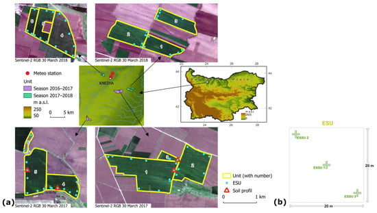
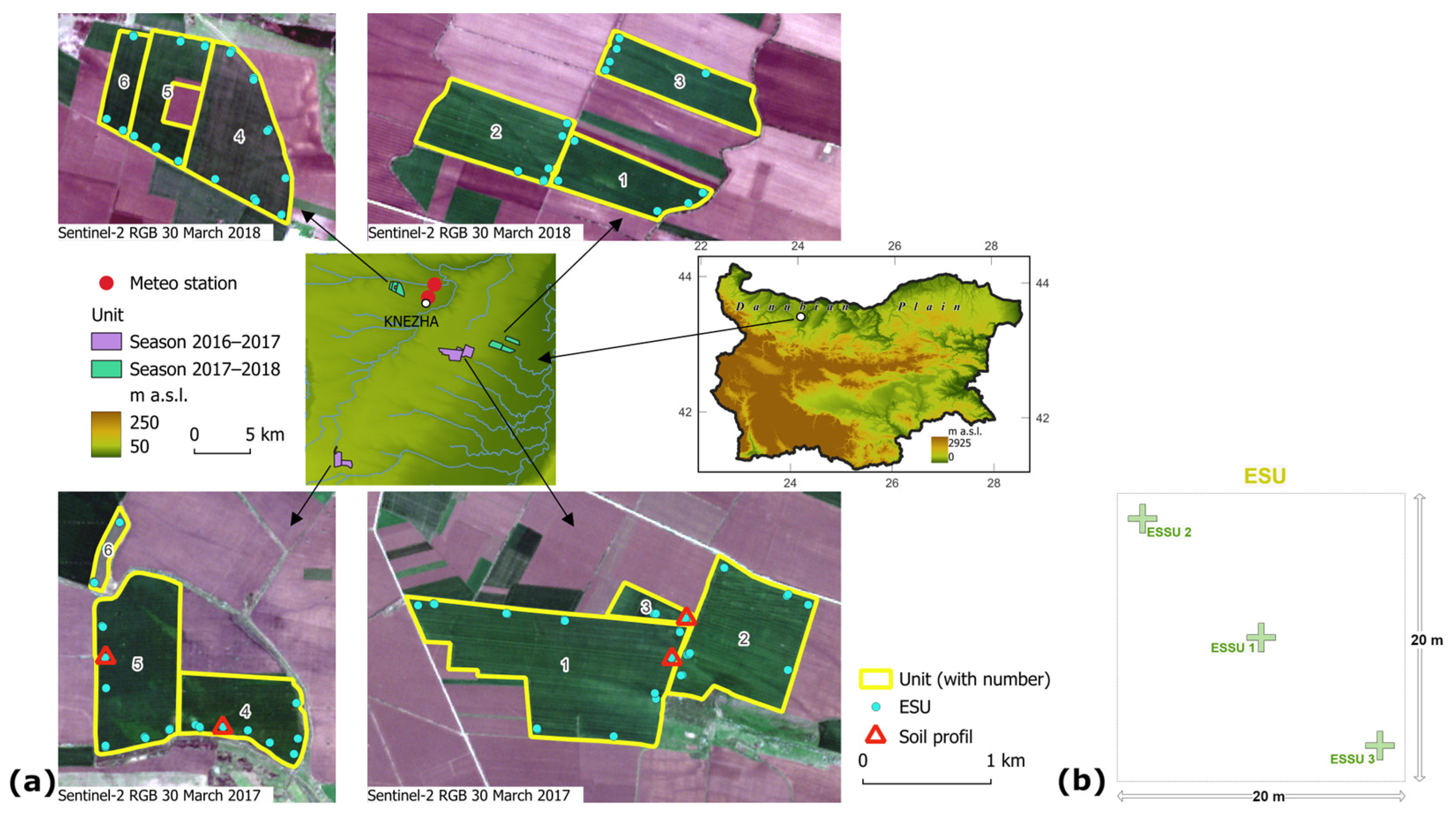
The study area (approximately 25 km × 25 km) is located in the Danubian Plain, Bulgaria (Figure 1a), near the town of Knezha. This part of the country represents one of the major agricultural regions and is characterized by low relief, fertile Chernozem soils, and a temperate continental climate with cold winters and hot summers. The mean annual temperature in Knezha is 11.1 °C, and the annual precipitation sum is 529 mm, with a maximum in May (www.stringmeteo.com (accessed on 7 November 2025)). The field campaigns were conducted in two agricultural seasons, 2016–17 and 2017–18. The campaigns lasted four to five days. In the first season, the campaigns were conducted in early November, late March, late April, mid-May, and late June (Table 1). In the second season, the campaigns were conducted in early November and early April.
Figure 1.
(a) Location of the study area and the Units sampled in each of the two agricultural seasons. (b) Scheme of an Elementary Sampling Unit (ESU) showing the distribution of the three Elementary Sub Sampling Units (ESSU), shown as crosses.
Table 1.
Dates of the field campaigns and the corresponding development stage of winter wheat.
A hierarchical sampling strategy consisting of three levels was adopted: Unit (a single commercial agricultural field), Elementary Sampling Unit (ESU; a 20 m × 20 m plot), and Elementary Sub-Sampling Unit (ESSU; a specific location within the ESU where measurements are taken). Six Units were selected each season (12 in total; total area 647 ha; Figure 1a) and sampled during all field campaigns in the same season. Selection was based on the availability of farmers to cooperate, ease of access, and winter wheat variety: three Units, each sown with the Enola and Anapurna varieties. The ESUs were selected to represent different soil varieties (at least 3 ESUs per soil variety) and were spaced at least 50 m apart and 30–50 m from the Unit boundary. During each field campaign, 30 ESUs were measured, but some parameters may not be available for each of them (see Section 4.1. Missing data for more details and Table 2 for the actual number of sampled ESUs per parameter). The geographic coordinates in the center of each ESU were recorded using a GPS receiver, Magellan Mobile Mapper 6 (Magellan Navigation, Inc., San Dimas, CA, USA). The GPS was run in “averaging” mode for 5 min, and raw data were collected for post-processing. In general, the location of the ESUs was kept unchanged between the field campaigns. As an exception, some ESUs were relocated due to waterlogging. The geographic coordinates were measured (and reported in the dataset) each time an ESU was visited (except in June 2017, when the last field campaign coordinates were used), irrespective of whether it was relocated or not. In each ESU, there were 3 ESSUs (Figure 1b) where actual measurements/observations took place. This allowed us to account for and quantify the variability within the ESU. Final data are reported at the ESU level only, with averages across ESSUs. The exception was the biological yield, which was determined only in the central ESSU, and this value was reported for the ESU.
Table 2.
Summary of the parameters available at the Elementary Sampling Unit (ESU) level, including sample sizes (total number of ESUs) and temporal coverage (field campaigns).
Two unique identifiers, Unit_ID and ESU_ID, were used across the dataset’s tables to identify data records and link tables. The Unit_ID consists of the season and the Unit number; for instance, “S16-17_U1”, where “S16-17” is the agricultural season 2016–2017 and “U1” is Unit 1. The ESU_ID consists of the month and year of the field campaign, the Unit number, and the ESU number, for instance “apr2017_1_2”, where “apr2017” is the April 2017 field campaign, “1” is the Unit number, and “2” is the ESU number.
3.2. Data Collection
3.2.1. ESU DataLeaf Area Index (LAI)
Leaf Area Index (LAI)
The LAI data were collected using the AccuPAR LP-80 ceptometer (METER Group, Inc., Pullman, WA, USA; formerly Decagon Devices, Inc., Pullman, WA, USA). Generally, LAI is defined as one-half of the total green leaf area per unit horizontal ground surface area [2]. Several closely related terms are used in the literature depending on whether only green or also non-green plant parts are considered and whether only leaves or also other vegetation organs are taken into account [3]. The AccuPAR LP-80 cannot separate green leaves from senescent leaves and other plant organs, such as stem, inflorescence, etc., and does not explicitly account for the clumping of the canopy (i.e., the non-random distribution of canopy elements). Based on the Fang et al. [2] summary of LAI-related terms, the appropriate term for the quantity estimated by AccuPAR LP-80 is Effective Plant Area Index (PAIeff). Nevertheless, we use the term LAI in this paper because it is the term used by the manufacturer of the AccuPAR LP-80. Also, as the wheat canopy is rather random, except in early stages when rows are still discernible, clumping can be ignored. The AccuPAR LP-80 ceptometer measures the Photosynthetically Active Radiation (PAR; 400–700 nm waveband) using 80 sensors placed along a linear probe. By taking above and below canopy measurements, the instrument quantifies light interception in plant canopies and inverts these readings to give LAI [4]. To calculate LAI, AccuPAR LP-80 requires the leaf angle distribution parameter (χ) to be set. We set it to 0.96, which is the value suggested for wheat [5]. An external PAR sensor is included with the AccuPAR to enable simultaneous above- and below-canopy PAR measurements. The external sensor was used for most measurements, particularly those made under rapidly changing illumination conditions. The AccuPAR LP-80 was calibrated once a day (at the beginning of measurements) using the external sensor, which is the PAR standard to which the probe is calibrated [4]. To obtain a good representation of the below-canopy PAR, 10 measurements were taken at each location (i.e., ESSU), and the average was calculated using the AccuPAR LP-80. The 10 measurements were taken by placing the probe perpendicular to the crop rows at ~10 cm intervals, thus forming a sampling plot of roughly 1 m2.
Fraction of Absorbed Photosynthetically Active Radiation (fAPAR)
AccuPAR LP-80 was used to collect data for calculating fAPAR. The following equations were used (Equations (3), (6) and (7) from [4]):
where t is the fraction of incident radiation transmitted by the canopy, r is the fraction of incident radiation reflected to a sensor above the canopy, rs is the reflectance of the soil surface (we assume rs = 0.15), S is the PAR reading from an upward-facing AccuPAR LP-80 above the plant canopy, R is the reflected PAR above the plant canopy (inverted AccuPAR LP-80 above the crop), and T is the PAR reading from an upward-facing AccuPAR below the plant canopy. To obtain a good representation of the below-canopy PAR (i.e., T), 10 measurements were taken at each location (i.e., ESSU), and the average was calculated using the AccuPAR LP-80. The 10 measurements were taken by placing the probe perpendicular to the crop rows at ~10 cm intervals, thereby forming a sampling plot of roughly 1 m2.
The last two terms in Equation (1) can be ignored, in which case the fraction of Intercepted Photosynthetically Active Radiation (fIPAR) is obtained [4]:
Both fAPAR and fIPAR were calculated.
Vegetation Cover Fraction (fCover)
AccuPAR LP-80 was used to collect data for calculating fCover. Vegetation cover fraction (fCover; also called Fractional Vegetation Cover, FVC [6]) is defined as the vertical projection area of aboveground vegetation elements per unit horizontal ground surface area [7]. The fCover calculation is possible with the AccuPAR LP-80 because measurements of t at one zenith angle can be used to predict transmission or radiation interception at other zenith angles [4]. If we are interested in fCover, then we should predict t for the zenith angle , i.e., , using the actual measured t, :
where χ is the leaf angle distribution parameter (for wheat χ = 0.96) and is the actual zenith angle during the measurement (in radians). fCover is then (). For how p is derived, see the AccuPAR LP-80 Operator’s Manual [4]. The calculations were made in a spreadsheet using the same data used to calculate LAI and fAPAR.
Chlorophyll Content (CC)
The leaf CC data were collected using the Chlorophyll Content Meter CCM-300 (Opti-Sciences, Inc., Hudson, NH, USA). CCM-300 works by measuring the Chlorophyll Fluorescence Ratio—fluorescence emission ratio of intensity at 735 nm/700 nm, which is highly correlated with chlorophyll content [8]. The instrument provides a direct readout of chlorophyll content in mg·m−2. Two measurements were taken from the uppermost fully developed leaf of at least five plants in each ESSU. Data were converted to μg·cm−2.
Above-Ground Biomass
All plants were cut at the ground surface from a 1 m2 plot at the central ESSU and from 50 cm × 50 cm plots in the other two ESSUs. Winter wheat and weeds were separated and stored in plastic bags. The fresh weight (AGBf in g·m−2) of the samples was measured at the end of the working day. At the end of the field campaign, they were transported to the laboratory of the Institute of Soil Science, Agrotechnologies and Plant Protection “Nikola Poushkarov” in Sofia, where dry biomass (AGBd in g·m−2) was determined after drying at 60 °C to constant weight.
Plant Nitrogen (N) Content and Uptake
The N content of the above-ground organs (leaf and stem) was determined by the Kjeldahl method [9] and expressed as a percentage of the dry weight. The N uptake (g·m−2) was determined as the product of N content and AGBd. The analyses were carried out at the laboratory of the Institute of Soil Science, Agrotechnologies and Plant Protection “Nikola Poushkarov” in Sofia. The analyzed plant material was collected from the above-ground biomass samples.
Biological Yield
The biological yield data were collected only at the end of June, during the first agricultural season. All plants were harvested from a 1 m2 plot at the central ESSU. Initially, the ears were separated from each plant. A thresher designed for field trial samples was used to separate the grain from the ears. The separated grain was measured on an electronic scale. Biological yield, in dry weight, was obtained in the laboratory of the Institute of Soil Science, Agrotechnologies and Plant Protection “Nikola Poushkarov” in Sofia after drying the sample at 60 °C.
Surface Soil Moisture
Soil moisture content (W) was measured gravimetrically at the surface layer (0–5 cm) and, in some ESUs, at three additional depths (0–30 cm, 30–60 cm, and 60–100 cm) in 10 cm increments. The data were expressed in percent by mass. Additionally, the soil type in each ESU was determined based on the large-scale (1:10,000) national soil map. The map uses the national classification [10]; therefore, the Bulgarian soil types were correlated with the World Reference Base for Soil Resources (WRB) classification system [11].
Spectroradiometer Data
Reflectance data in the spectral range of 350–2500 nm were collected using an ASD FieldSpec 4 Hi-Res Field Spectrometer (ASD Inc., Boulder, CO, USA). The instrument provides a spectral resolution of 3 nm in the 350–1000 nm range and 8 nm in the 1000–2500 nm range, with the output spectra internally resampled to 1 nm intervals. Prior to measurements, the device was powered on for 15–30 min to allow thermal stabilization.
All measurements were acquired in relative reflectance units. A Spectralon white reference panel was used for calibration and measured before each ESSU acquisition. The instrument was operated with a bare fiber, providing a 25° field of view. When positioned at a nadir 135 cm above the canopy, this setup corresponds to a circular ground footprint with a diameter of approximately 60 cm [12].
Phenological Observations and Other Measurements
A set of phenological observations and measurements was made in a 1 m2 plot at the central ESSU and 50 cm × 50 cm plots in the other two ESSUs, as with the biomass sampling. They included:
- Expert assessment of the development stage after the Zadoks growth scale [1].
- Plant density (number of winter wheat plants per square meter).
- Plant height (cm) measured from the base of the stem (at the soil surface) to the top of the canopy with a wooden meter. Six measurements were made in each ESSU.
- Expert assessment of total area coverage (%).
- Expert assessment of damages caused by diseases or pests using a five-point rating scale: (1) heavy damages above 50%, (2) medium damages between 25 and 50%, (3) slight damages between 10 and 25%, (4) very slight damages below 10%, and (5) no damages.
- Weed (including self-seeded crops) characterization: determining the type, development stage, height (cm), and overall weed score. The weed score was assessed using a five-point rating scale: (1) weeds only, no cultivated plants, (2) weeds prevail over the cultivated plants and suffocate them, (3) many weeds, but cultivated plants still prevail, (4) isolated weeds, and (5) no weeds.
Table 2 summarizes the available data measured in ESUs, providing for each parameter the total number of ESUs in which it was measured and the field campaigns in which the measurements were conducted. For example, LAI was measured in 168 ESUs; these data come from six different field campaigns.
3.2.2. Auxiliary DataCrop Calendar and Management
Crop Calendar and Management
The following data were collected for each Unit:
- Basic data—area (ha), soil type according to the WRB classification system [11], land category, predecessor, pre-sowing preparation, variety, sowing (date, norm).
- Soil fertilization (date, type, amount)—pre-sowing and spring fertilization, foliar feeding.
- Plant protection measures (date, type, amount)—treating crops with herbicides and fungicides.
- Crop calendar of winter wheat—development stage after the Zadoks growth scale [1]: Germination, Main stem leaf production, Tiller production, Restoration of vegetation after overwintering, Stem elongation, Heading, Anthesis, Grain milk stage, Grain dough stage, Ripening. The recorded development stage date corresponds to the date when 75% of the plants in each Unit were in the corresponding stage.
- Harvesting date and yield (kg·ha−1) provided by the farmer.
Table 3 provides a subset of the data.
Table 3.
Basic information for the sampled Units.
Soil Profiles
In the first agricultural season, 2016–17, four soil profiles (Units 1, 3, 4, and 5; Figure 1a) were studied by digging open pits. The profiles were located to cover all terrain elements and the main soil types. The pits were rectangular, measuring 200 cm long, 100 cm wide, and 150 cm deep. The genetic horizons were defined and described based on the shorter side of the profile, which, at the time of observation, was well exposed to direct sunlight. The morphological description of each genetic horizon includes Munsell soil color, structure, texture, humidity, included elements, and newly formed elements.
The particle-size distribution was determined by sieving and the pipette method [13]. Fractions of sand (2–0.063 mm), silt (0.063–0.002 mm), and clay (<0.002 mm) were determined for the textural classification according to [11]. The concentration of organic carbon (SOC, %) was determined using the modified Tjurin method [14,15]. The soil acidity was measured in a 1:2.5 soil/water suspension using a pH meter.
Vertically oriented soil cores were sampled in 4 replicates in 100 cm3 metal cylinders to determine bulk density (Db) and water retention at suction levels from 0.25 kPa (pF 0.4) to 33 kPa (pF 2.7). The soil bulk density data can be used to calculate volumetric water content (VWC). , where W is the gravimetric water content. The total porosity (Pt) was calculated using the measured bulk soil density (Db) and particle density (Ds = 2.65 g·cm−3):
The data can be used to calculate percent saturation (). Soil water retention curves (pF curves) were obtained by draining samples using the suction plate method, the pressure membrane apparatus, and the desiccator method, as described by Rousseva et al. [16]. The field capacity (FC) was estimated by the water content retained at a suction of 10 kPa (pF = 2.0). The wilting point was estimated at a suction of 1500 kPa (pF = 4.2). The water retention experimental data at different suctions were approximated with the van Genuchten equation [17]:
where W is gravimetric water content (kg·kg−1), h is suction (hPa), Wsat is water content at saturation, Wres is residual water content (h → ∞), α (hPa−1), and n and m are fitted parameters. Stable results for the parameters were obtained when a constraint was applied for m = 1 − 1/n [18] and when the parameter Wres was fixed to zero in cases with estimated negative values. The parameters Wsat, Wres, α, and n were fitted using statistical regression methods in OriginPro 6.1.
Multispectral UAV Imagery
Multispectral image mosaics of the Units were generated during each field campaign (except June 2017) using a fixed-wing drone, eBee Ag (EagleNXT, Wichita, KS, USA; formerly senseFly, Cheseaux-Lausanne, Switzerland), equipped with a Sequoia camera (Parrot Drones SAS, Paris, France). The camera has RGB (data not included in the dataset) and a multi-channel sensor with green (550 nm), red (660 nm), red edge (735 nm), and NIR (790 nm) bands [19]. The band width is 40 nm (10 nm for the red edge band). A sunshine sensor mounted on the upper part of the camera records irradiance conditions during flight in the same spectral regions as the camera. The eBee Ag was flown in autopilot mode. Predefined flight plans were generated with the eMotion 2 software (EagleNXT, Wichita, KS, USA; formerly senseFly, Switzerland). In the usual case, more than one flight was needed to cover a single Unit. Two to three days were needed to image all Units; however, each Unit was imaged within a single day. Flights were conducted between 10:00 and 14:00 local time. During the first field campaign (November 2016), the flights were conducted at 106 m above ground with 75% forward and side overlap, resulting in a high ground resolution (10 cm per pixel) and a large number of images to be mosaicked in the post-processing stage. For the subsequent field campaigns, the ground resolution was reduced to 25 cm per pixel, corresponding to a flight height of 265 m and 80% forward and side overlap. Several Ground Control Points (GCPs) were marked permanently in the field and measured with GNSS Leica GS08+. The Pix4Dmapper software (Pix4D S.A., Prilly, Switzerland) was used for radiometric image processing (converting image values to surface reflectance based on the camera’s sunshine sensor data), orthorectification, and mosaicking. The GCPs were used to further improve the georeference of the mosaics in GIS.
Meteorological Data
Meteorological data were collected by an automatic telemetric agro-meteorological station, addVantage Pro6.5 (ADCON, Klosterneuburg, Austria), installed in the vicinity of the town of Knezha. The station operated between 30 November 2016 and 22 March 2017 at its initial location (Location 1: 43.521917° N, 24.098848° E) and was later moved 1.3 km southward to Location 2 (43.511391° N, 24.092252° E), where it collected data between 26 April 2017 and 3 December 2018. The station was equipped with: GPRS Data logger (ADCON, Austria), solar panel, combined temperature and relative humidity sensor Standard (ADCON, Austria), solar radiation sensor SP-LITE (ADCON, Austria), wind speed and direction sensor DS-2 (Decagon Devices, Inc., Pullman, WA, USA), rain gauge (Senseca Italy Srl., Caselle di Selvazzano, PD, Italy; formerly Delta OHM Srl., Caselle di Selvazzano, PD, Italy), PAR sensor LPPAR04BL (Senseca Italy Srl., Italy; formerly Delta OHM Srl., Italy), and soil moisture and temperature probe 120 cm Moisture SDI-12 (Sentek, Adelaide, Australia), which collected data at 12 depths between 5 cm and 115 cm at 10 cm intervals. Data from all sensors were recorded and are available in the dataset at 30 min intervals.
4. Limitations of Data and Precautions for Use
4.1. Missing Data
The sample size for the different parameters measured in the ESUs (see Table 2) varies, as not all parameters were measured in each ESU during each field campaign. This is due either to the fact that the parameter is only relevant during a certain period of the season or a certain field campaign (e.g., biological yield), or to adverse weather conditions preventing field work. “NA” is used to indicate missing data in the dataset. During the field campaign in November 2017, UAV flights were carried out over Units 1, 2 and 3, but no mosaics were generated due to poor image quality, which prevented their photogrammetric processing. Meteorological data are missing for the period of 23 March 2017–25 April 2017, when the agrometeorological station was not operational due to the need to repair the soil and wind sensors and move to another location. The unplanned relocation was necessitated by construction plans near the old location. In addition, there was missing data for one or more parameters, most notably wind speed and direction, and soil moisture and temperature. Such gaps occurred infrequently and were usually shorter than a day; the longest period was 12 days. Missing data are marked with “NA” in the dataset. Possible reasons include sensor failure or a temporary lack of GSM service.
4.2. Sources of Error
There are various sources of error and noise in the field-collected data. These may be due to natural variation in soil properties within the field, crop heterogeneity, the moisture regime, plant diseases, weeds, and other factors. Among the main advantages of the proposed dataset are its repetitions and numerous field campaigns. However, the user should be aware of the following data imitations. Post-processing of the GPS coordinates of the ESUs was not possible for the field campaigns in March, April, and May 2017. Data from the other field campaigns show that the difference in the position of the original and post-processed points was mostly within 2 m, but in some cases it reached 4.5 m. However, this error is smaller than the ESU (20 m × 20 m). The uncertainty in the parameters measured using the AccuPAR LP-80, i.e., LAI, fAPAR, fIPAR, and fCover, can potentially be larger on sunny days. This is because keeping the linear probe and external PAR sensor completely level is crucial on sunny days. The variable “LP80_conditions” in the file “ESU_Biophysical_and_biochemical_crop_data.txt” provides information about the light conditions during each measurement, allowing users to select data collected under similar conditions (e.g., clear sky, cloud cover, etc.). The reader is referred to Garrigues et al. [20] for an analysis of the sensitivity of LAI retrievals from the AccuPAR LP-80 to light conditions. The CCM-300 uses calibration coefficients from the literature [8], but these are not developed specifically for winter wheat. Unfortunately, we were unable to perform our own calibration of the instrument.
5. Applications and Future Expansion Directions for Datasets
The most common applications for the obtained ground data are: validating satellite products; providing input data for simulation models that predict crop productivity, soil, water, and nutrient balance; calibrating and validating simulation models; drought risk analysis; and combining process-based models with deep learning. The remote sensing community has long recognized the need for georeferenced ground data to validate algorithms for estimating various land surface variables from satellite observations [21,22]. In recent decades, several test sites and networks have been established worldwide, where field measurements and aerial imagery are collected to support the validation of remote sensing products [23,24,25,26,27]. In addition to time-consuming field campaigns, wireless sensor networks have also been used, highlighting the growing need for efficient data collection [28]. Crop simulation models describe the processes in the crop–soil system as influenced by environmental conditions (weather patterns) and management practices adopted for crop cultivation [29]. The WOrld FOod STudies (WOFOST) model [30], for example, requires data on climate, soil profile, and soil physical characteristics, among other inputs, all of which are available in the presented dataset. Additionally, biomass and yield data are available, allowing for comparison of modeled crop production with actual field data [31] and for comparison of the relative performance of different models [32,33]. Crop simulation models estimate various canopy state variables, such as LAI, biomass, and fAPAR. Independent data for these variables, mostly from remote sensing, have been assimilated into crop models, improving their predictions [34]. In this context, our dataset can be used to test different assimilation approaches, such as crop model calibration, forcing methods, and updating methods [34]. Soil moisture content and soil profile data can be used to assess the performance of soil water balance models [35,36].
Given the potential utility of the dataset for various process-based models, it may be possible to expand it in the future by adding parameters once specific simulation models have been calibrated. It is also important to continue collecting field data in the future for other regions and crops. These future datasets should comply with community-agreed validation procedures, such as those of the Committee on Earth Observation Satellites (CEOS) Working Group on Calibration and Validation land product validation (LPV) subgroup [27]. In the coming years, the need for ground-based measurements whose uncertainty budget has been characterized will be increasingly emphasized [37]. If possible, such datasets should contain not only a single parameter of interest, such as LAI, but also a set of parameters characterizing crops, soil, and weather conditions, as well as UAV images, which would allow not only validation studies but also a better understanding of agricultural systems through modeling [38].
Author Contributions
Conceptualization, E.R. and D.G.; methodology, E.R.; investigation, P.D., E.R., G.J., L.F., A.G., I.K., I.I., M.K., M.B., V.K. (Veneta Krasteva), V.K. (Viktor Kolchakov), E.D. and N.M.; resources, M.B.; data curation, P.D., E.R. and M.K.; writing—original draft preparation, P.D., E.R. and M.K.; writing—review and editing, D.G. and L.F.; visualization, P.D.; supervision, E.R. and M.B.; project administration, P.D.; funding acquisition, E.R. and L.F. All authors have read and agreed to the published version of the manuscript.
Funding
The data described in this paper were collected as part of the “Testing Sentinel-2 vegetation indices for the assessment of the state of winter crops in Bulgaria” (TS2AgroBg) project funded by the European Space Agency (Contract No. 4000117474/16/NL/NDe) under the Plan for European Cooperating States.
Institutional Review Board Statement
Not applicable.
Informed Consent Statement
Not applicable.
Data Availability Statement
The dataset described in this paper is available from Zenodo: https://doi.org/10.5281/zenodo.17475742 (accessed on 7 November 2025) under the terms of the Creative Commons Attribution 4.0 International public license.
Acknowledgments
We thank the farmers and cooperatives who provided access to their fields and kindly assisted with fieldwork by providing transportation and space for sample storage and processing. They also provided information and data about the fields. We are grateful to agronomist Polina Marinska for her participation in fieldwork and for consulting the team.
Conflicts of Interest
The authors declare no conflicts of interest. The funders had no role in the design of the study; in the collection, analyses, or interpretation of data; in the writing of the manuscript; or in the decision to publish the results.
References
- Zadoks, J.C.; Chang, T.T.; Konzak, C.F. A decimal code of the growth stages of cereals. Weed Res. 1974, 14, 415–421. [Google Scholar] [CrossRef] [Scilit]
- Fang, H.; Baret, F.; Plummer, S.; Schaepman-Strub, G. An overview of global leaf area index (LAI): Methods, products, validation, and applications. Rev. Geophys. 2019, 57, 739–799. [Google Scholar] [CrossRef] [Scilit]
- Li, W.; Li, D.; Warner, T.A.; Liu, S.; Baret, F.; Yang, P.; Jiang, J.; Dong, M.; Cheng, T.; Zhu, Y.; et al. Improved generality of wheat green LAI models through mitigation of the effect of leaf chlorophyll content variation with red edge vegetation indices. Remote Sens. Environ. 2025, 318, 114589. [Google Scholar] [CrossRef] [Scilit]
- AccuPAR PAR/LAI Ceptometer Model LP-80 Operator’s Manual. Version December 13. Decagon Devices. 78p. 2013. Available online: https://www.labcell.com/media/84704/lp-80%20manual%20v11.pdf (accessed on 7 November 2025).
- Campbell, G.S.; Norman, J.M. An Introduction to Environmental Biophysics, 2nd ed.; Springer: New York, NY, USA, 1998; p. 286. [Google Scholar]
- Yan, G.; Mu, X.; Jia, K.; Song, W.; Liu, Y.; Chen, J.; Gao, Z. Fractional vegetation cover. In Advanced Remote Sensing, 2nd ed.; Liang, S., Wang, J., Eds.; Academic Press: New York, NY, USA, 2020; pp. 477–510. [Google Scholar] [CrossRef] [Scilit]
- Li, L.; Mu, X.; Jiang, H.; Chianucci, F.; Hu, R.; Song, W.; Qi, J.; Liu, S.; Zhou, J.; Chen, L.; et al. Review of ground and aerial methods for vegetation cover fraction (fCover) and related quantities estimation: Definitions, advances, challenges, and future perspectives. ISPRS J. Photogramm. Remote Sens. 2023, 199, 133–156. [Google Scholar] [CrossRef] [Scilit]
- Gitelson, A.A.; Buschmann, C.; Lichtenthaler, H.K. The Chlorophyll Fluorescence Ratio F735/F700 as an Accurate Measure of Chlorophyll Content in Plants. Remote Sens. Environ. 1999, 69, 296–302. [Google Scholar] [CrossRef] [Scilit]
- Sáez-Plaza, P.; Navas, M.J.; Wybraniec, S.; Michałowski, T.; Asuero, A.G. An Overview of the Kjeldahl Method of Nitrogen Determination. Part II. Sample Preparation, Working Scale, Instrumental Finish, and Quality Control. Crit. Rev. Anal. Chem. 2013, 43, 224–272. [Google Scholar] [CrossRef] [Scilit]
- Yolevski, M.; Hadzhiyanakiev, A. Agro-grouping of soils in Bulgaria, Extended systematic list. In Code of Groups and Soil Varieties; Institute of Soil Science Nikola Poushkarov: Sofia, Bulgaria, 1976. (In Bulgarian) [Google Scholar]
- IUSS Working Group WRB. World Reference Base for Soil Resources 2014. International Soil Classification System for Naming Soils and Creating Legends for Soil Maps. World Soil Resources Reports No. 106; FAO: Rome, Italy, 2014. [Google Scholar]
- Hatchell, D.C. (Ed.) ASD Technical Guide, 4th ed.; ASD: Boulder, CO, USA, 2009. [Google Scholar]
- ISO 11277–2020; Soil quality—Determination of particle size distribution in mineral soil material—Method by sieving and sedimentation. International Organization for Standardization: Geneva, Switzerland, 2020.
- Kononova, M.M. Soil Organic Matter: Its Nature, Its Role in Soil Formation and in Soil Fertility, 2nd ed.; Pergamon Press: Oxford, UK, 2013. [Google Scholar]
- Filcheva, E.G.; Tsadilas, C.D. Influence of Clinoptilolite and Compost on Soil Properties. Commun. Soil Sci. Plant Anal. 2002, 33, 595–607. [Google Scholar] [CrossRef] [Scilit]
- Rousseva, S.; Kercheva, M.; Shishkov, T.; Lair, G.J.; Nikolaidis, N.P.; Moraetis, D.; Krám, P.; Bernasconi, S.M.; Blum, W.E.H.; Menon, M.; et al. Soil Water Characteristics of European SoilTrEC Critical Zone Observatories. In Advances in Agronomy; Academic Press: Cambridge, MA, USA, 2017; Volume 142, pp. 29–72. [Google Scholar]
- van Genuchten, M.T. A closed-form equation for predicting the hydraulic conductivity of unsaturated soils. Soil Sci. Soc. Am. J. 1980, 44, 892–898. [Google Scholar] [CrossRef] [Scilit]
- Mualem, Y. A new model predicting the hydraulic conductivity of unsaturated porous media. Water Resour. Res. 1976, 12, 513–522. [Google Scholar] [CrossRef] [Scilit]
- Parrot Sequoia User Guide. Available online: https://www.parrot.com/assets/s3fs-public/2021-09/sequoia-userguide-en-fr-es-de-it-pt-ar-zn-zh-jp-ko_1.pdf (accessed on 7 November 2025).
- Garrigues, S.; Shabanov, N.V.; Swanson, K.; Morisette, J.T.; Baret, F.; Myneni, R.B. Intercomparison and sensitivity analysis of Leaf Area Index retrievals from LAI-2000, AccuPAR, and digital hemispherical photography over croplands. Agric. For. Meteorol. 2008, 148, 1193–1209. [Google Scholar] [CrossRef] [Scilit]
- Morisette, J.T.; Baret, F.; Privette, J.L.; Myneni, R.B.; Nickeson, J.E.; Garrigues, S.; Shabanov, N.V.; Weiss, M.; Fernandes, R.A.; Leblanc, S.G.; et al. Validation of global moderate-resolution LAI products: A framework proposed within the CEOS land product validation subgroup. IEEE Trans. Geosci. Remote Sens. 2006, 44, 1804–1817. [Google Scholar] [CrossRef] [Scilit]
- Kancheva, R.; Borisova, D.; Georgiev, G. In-situ networks on test-sites in support of space earth observations. In First Workshop on Hyperspectral Image and Signal Processing: Evolution in Remote Sensing; IEEE: Grenoble, France, 2009; pp. 1–4. [Google Scholar] [CrossRef] [Scilit]
- Gerighausen, H.; Borg, E.; Wloczyk, C.; Fichtelmann, B.; Günther, A.; Vajen, H.-H.; Rosenberg, M.; Schulz, M.; Engler, H.-G. DEMMIN—A test site for the validation of Remote Sensing data products. General description and application during AgriSAR 2006. In Proceedings of the AGRISAR and EAGLE Campaigns Final Workshop, Noordwijk, The Netherlands, 15–16 October 2007; Available online: https://elib.dlr.de/53957/1/03_01_Borg.pdf (accessed on 23 January 2026).
- Ma, M.G.; Li, X.; Weizhen, W.; Xiao, Q.; Zhao, K.; Xin, X.P. Design on validation network of remote sensing products in China. Int. Arch. Photogramm. Remote Sens. Spat. Inf. Sci. 2013, 40, 1–6. [Google Scholar] [CrossRef] [Scilit]
- Wang, S.; Li, X.; Ge, Y.; Jin, R.; Ma, M.; Liu, Q.; Wen, J.; Liu, S. Validation of Regional-Scale Remote Sensing Products in China: From Site to Network. Remote Sens. 2016, 8, 980. [Google Scholar] [CrossRef] [Scilit]
- Baret, F.; Weiss, M.; Allard, D.; Garrigue, S.; Leroy, M.; Jeanjean, H.; Fernandes, R.; Myneni, R.; Privette, J.; Morisette, J.; et al. VALERI: A Network of Sites and a Methodology for the Validation of Medium Spatial Resolution Land Satellite Products. 2021. Available online: https://hal.inrae.fr/hal-03221068 (accessed on 26 January 2026).
- Camacho, F.; Sánchez-Zapero, J.; Martínez-Sanchez, E. Chapter 6—Standardized validation of satellite-based biogeophysical products. In Earth Observation, Carbon Fluxes and Biophysical Variables from Earth Observation; Campos-Taberner, M., Martínez, B., Sánchez-Ruiz, S., Eds.; Elsevier: Amsterdam, The Netherlands, 2025; pp. 153–205. [Google Scholar] [CrossRef] [Scilit]
- Li, X.; Liu, Q.; Yang, R.; Wen, J.; Zhang, J.; Cai, E.; Zhang, H. The Combination of Ground-Sensing Network and Satellite Remote Sensing in Huailai County. IEEE Sens. J. 2016, 16, 3819–3826. [Google Scholar] [CrossRef] [Scilit]
- Banerjee, K.; Dutta, S.; Das, S.; Sadhukhan, R. Crop simulation models as decision tools to enhance agricultural system productivity and sustainability—A critical review. Technol. Agron. 2025, 5, e002. [Google Scholar] [CrossRef] [Scilit]
- van Diepen, C.A.; Wolf, J.; van Keulen, H.; Rappoldt, C. WOFOST: A simulation model of crop production. Soil Use Manag. 1989, 5, 16–24. [Google Scholar] [CrossRef] [Scilit]
- Dewenam, L.E.F.; Er-Raki, S.; Ezzahar, J.; Chehbouni, A. Performance Evaluation of the WOFOST Model for Estimating Evapotranspiration, Soil Water Content, Grain Yield and Total Above-Ground Biomass of Winter Wheat in Tensift Al Haouz (Morocco): Application to Yield Gap Estimation. Agronomy 2021, 11, 2480. [Google Scholar] [CrossRef] [Scilit]
- Zheng, J.; Yu, L.; Du, Z.; Xiao, L.; Huang, X. Modeling wheat development under extreme weather with WOFOST-EW v1. Geosci. Model Dev. 2025, 18, 8379–8400. [Google Scholar] [CrossRef] [Scilit]
- Singh, J.; Biswas, B.; Dhaliwal, L.K.; Poddar, R.; Gharib, A.F.; Raafat, B.M.; Gaber, A.; Hossain, A. Performance evaluation of the DSSAT-CERES-Wheat and WOFOST-Wheat models under various agroclimatic conditions in northwest India. Theor. Appl. Clim. 2025, 156, 250. [Google Scholar] [CrossRef] [Scilit]
- Jin, X.; Kumar, L.; Li, Z.; Feng, H.; Xu, X.; Yang, G.; Wang, J. A review of data assimilation of remote sensing and crop models. Eur. J. Agron. 2018, 92, 141–152. [Google Scholar] [CrossRef] [Scilit]
- Yi, J.; Li, H.; Zhao, Y.; Shao, M.; Zhang, H.; Liu, M. Assessing soil water balance to optimize irrigation schedules of flood-irrigated maize fields with different cultivation histories in the arid region. Agric. Water Manag. 2022, 265, 107543. [Google Scholar] [CrossRef] [Scilit]
- Aggarwal, P.; Bhattacharyya, R.; Amit Kumar Mishra, A.K.; Das, T.K.; Šimůnek, J.; Pramanik, P.; Sudhishri, S.; Vashisth, A.; Krishnan, P.; Chakraborty, D.; et al. Modelling soil water balance and root water uptake in cotton grown under different soil conservation practices in the Indo-Gangetic Plain. Agric. Ecosyst. Environ. 2017, 240, 287–299. [Google Scholar] [CrossRef] [Scilit]
- Goryl, P.; Fox, N.; Donlon, C.; Castracane, P. Fiducial Reference Measurements (FRMs): What Are They? Remote Sens. 2023, 15, 5017. [Google Scholar] [CrossRef] [Scilit]
- Jones, J.W.; Antle, J.M.; Basso, B.; Boote, K.J.; Conant, R.T.; Foster, I.; Godfray, H.C.J.; Herrero, M.; Howitt, R.E.; Janssen, S.; et al. Brief history of agricultural systems modeling. Agric. Syst. 2017, 155, 240–254. [Google Scholar] [CrossRef] [Scilit]

Disclaimer/Publisher’s Note: The statements, opinions and data contained in all publications are solely those of the individual author(s) and contributor(s) and not of MDPI and/or the editor(s). MDPI and/or the editor(s) disclaim responsibility for any injury to people or property resulting from any ideas, methods, instructions or products referred to in the content. |
© 2026 by the authors. Licensee MDPI, Basel, Switzerland. This article is an open access article distributed under the terms and conditions of the Creative Commons Attribution (CC BY) license.