Data Descriptor

Industrial Component Rolling-Test Order Spectra with Paired Mixed, Synchronous, and Master Exports


by
Krisztián Horváth
Department of Vehicle Development, Audi Hungaria Faculty of Engineering, Széchenyi István University, 9026 Győr, Hungary
Data 2026, 11(10), 264; https://doi.org/10.3390/data11100264
Submission received: 10 September 2026 / Revised: 29 September 2026 / Accepted: 1 October 2026 / Published: 3 October 2026

Abstract

Industrial rolling tests produce large collections of component-level vibration spectra, but their reuse depends on preserving measurement relationships and distinguishing repeat tests from repeated exports. This Data Descriptor presents 13 anonymized industrial component rolling-test Parquet exports acquired between January and April 2025, comprising 651,178 export rows and 645,951,488 spectral ordinates. The collection includes mixed and synchronous specimen spectra, maximum- and mean-labeled exports, and synchronous master spectra. Complete pseudonymous identifiers distinguish 54,920 Population A components and 54,396 Population B components. The workflow preserves native order axes, removes redundant exports, validates event-level joins, and selects the earliest valid event per component and channel. Across four representative channels, median coordinate-wise standard deviations range from 2.67 to 4.57 dB, and median central 90% spans range from 8.61 to 9.65 dB. These results describe observed component-to-component variability under production rolling-test conditions; undetermined bench repeatability and reproducibility prevent separation of manufacturing, measurement, fixturing, and operating contributions. Quality checks identify 42 rows without component identifiers and one nonfinite spectral ordinate. An illustrative bearing-order analysis shows that restricting mixed spectra to shared coordinates changes a narrow-window flag rate from 94.76% to 0.98%; these flags are methodological diagnostics, not verified fault labels. The dataset supports descriptive spectral analysis, processing comparisons, and leakage-aware model development, subject to the documented acquisition and metadata limitations.
Dataset License: Creative Commons Attribution 4.0 International (CC BY 4.0)

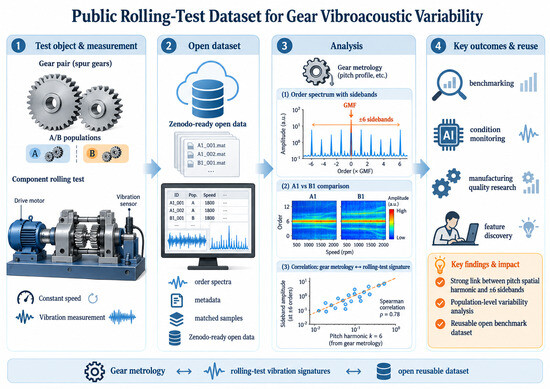
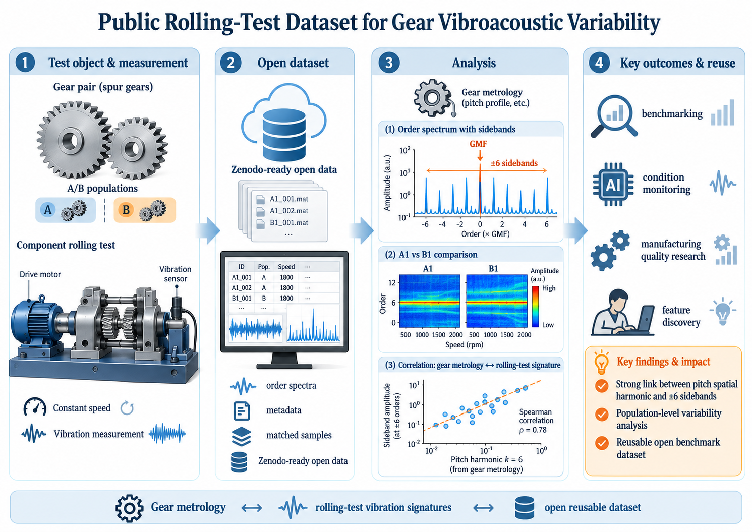
Graphical Abstract

1. Summary

Component rolling tests provide measurements of individual manufactured parts before their incorporation into an assembled drive. In this study, the term component-level rolling-test inspection refers to this pre-assembly measurement context. It is distinct from end-of-line testing of an assembled drive: component identifiers, excitation paths, fixture conditions, and inspection outcomes cannot automatically be transferred between the two contexts. The data described here [1] were supplied as industrial spectrum exports and are organized around the original source-channel labels. Their value lies in the large component population and in the availability of several processing representations associated with the same measurement events.
A reusable data resource needs more than a collection of spectral arrays. Users must know which rows refer to independent components, which are subsequent inspections, and which repeat an already exported measurement. They also need the actual order coordinates and the relationship between measurement channels. These requirements are consistent with the emphasis on metadata and reusable research objects in the FAIR principles [2]. In bearing diagnostics, a benchmark’s sampling conditions and interpretation limits also matter: the detailed assessment of the Case Western Reserve University dataset by Smith and Randall [3] provides an example of why diagnostic performance should be interpreted within the conditions represented by a dataset. The present collection supplies observational industrial spectra; it does not provide experimentally assigned bearing-defect classes. Recent cross-asset anomaly-detection and cross-machine bearing-diagnosis studies further demonstrate that distribution shift, heterogeneous machines, and differing operating conditions can materially affect generalization and may require explicit calibration or domain adaptation [4,5]. The order-tracking literature likewise shows that interpretation of rotating-machine spectra depends on the rotational reference, angular resampling, and analysis settings; these assumptions can materially affect the resulting order representation [6,7].
This descriptor has three purposes. First, it establishes a file-level and event-level description of a fixed, auditable 13-file core. Second, it quantifies observed component-to-component spectral variability while preserving the distinction between components, test events, and processing representations. Third, it illustrates how choices in order-coordinate selection can change an apparently simple bearing-related indicator. The latter example supports careful reuse of the spectra; it does not establish that the production components or the test rig had contaminated or defective bearings.
The public Version 1.0 release is intentionally limited to the validated 13-file core. Three additional source exports are not included in Version 1.0, and no sample counts or signal-processing results from those files are reported here. A future dataset version may extend the inventory after the additional exports and their metadata have been validated. The present descriptor therefore refers only to the fixed public 13-file release.

2. Data Description

2.1. Scope, Storage, and Observation Units

The 13-file core comprises 651,178 rows, 645,951,488 spectral ordinates, and 2,600,865,968 bytes (approximately 2.60 GB; 2.42 GiB) of compressed Parquet data. The observed timestamp range is 9 January 2025, 12:01:01, to 17 April 2025, 04:30:40. The timestamps are reported as stored; their timezone is not established by the supplied metadata. Parquet is a column-oriented file format [8], allowing metadata columns or selected spectral columns to be read without requesting every column. The files are derived spectrum exports and should not be described as raw acquisition time histories.
Table 1 lists the validated files using neutral analytical labels. The Zenodo record includes README.md, DATA_DICTIONARY.md, CITATION.cff, and SHA256SUMS.txt; the checksum manifest provides SHA-256 hashes for the 13 public Parquet files. Population A and Population B denote the two pseudonymized measurement populations; State A1, State B1, State A0, and State B0 are neutral analytical state labels. MIX, SYNCH, TAC, MAX, and MW are retained only as generic processing or response descriptors required to distinguish the released representations; the source-specific secondary response-channel label is replaced by the neutral term response B. None of these labels should be interpreted as a public product designation, drawing code, manufacturing line, or proprietary design specification. The terms specimen and master are descriptive labels for the two measurement representations used in the analysis. Detailed industrial semantics are intentionally not disclosed beyond the information required to interpret the public dataset.
Across the fixed 13-file core, two pseudonymous component-type codes and two pseudonymous test-bench codes are present. Each individual file contains one component-type value and one test-bench value. These cardinalities are reported to clarify dataset structure without disclosing the original industrial identifiers.
Export rows, measurement events, and components are different observation units. One component may have measurements in several channels, and one measurement may appear more than once in an export. The Population A specimen population contains 54,920 components with complete pseudonymous identifiers. Population B contains 54,396 components with complete pseudonymous identifiers after incomplete identifiers are excluded. The Population A and Population B pseudonymous component-ID sets have no overlap in this core; this observation establishes no match between those sets under the supplied identifier scheme. It does not establish a cross-system traceability rule or a link to an assembled-drive dataset.
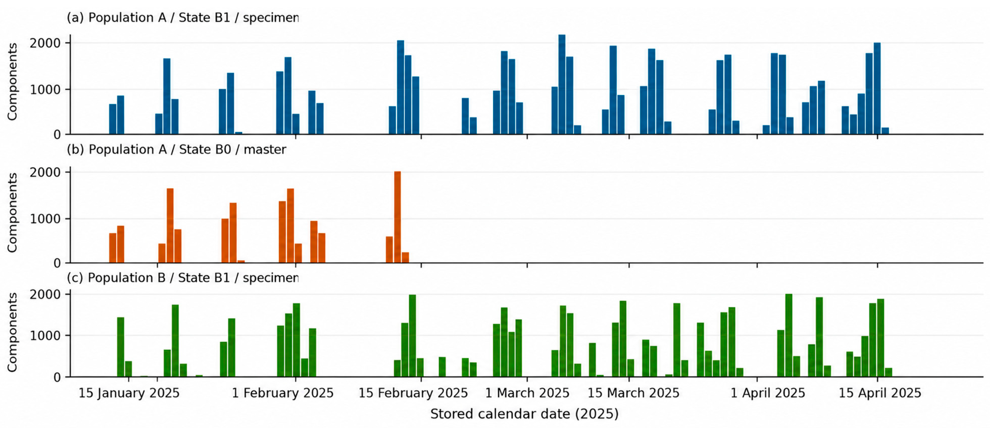
The master exports contain 14,962 components with complete pseudonymous identifiers and cover the early part of the observation period, ending on 13 February 2025. Their event identifiers match a subset of the Population A specimen events. Consequently, the master counts must not be added to the specimen counts as if they described additional independent components. Figure 1 displays the daily number of first-observed components for representative specimen and master channels. A first observation is the earliest accessible event for a component within that channel, not necessarily its first-ever industrial inspection.

2.2. Schema, Axes, and Physical Quantities

Each export starts with seven metadata columns: time, serial_number, type, test_bench, test_result, group, and ord. All subsequent columns have numeric names that encode the spectral coordinates. Table 2 defines the schema used by the analysis. The ord column is a sparsely populated unit annotation; it is neither a measurement identifier nor the numerical axis. Reading it as the order vector would therefore produce an incorrect data model.
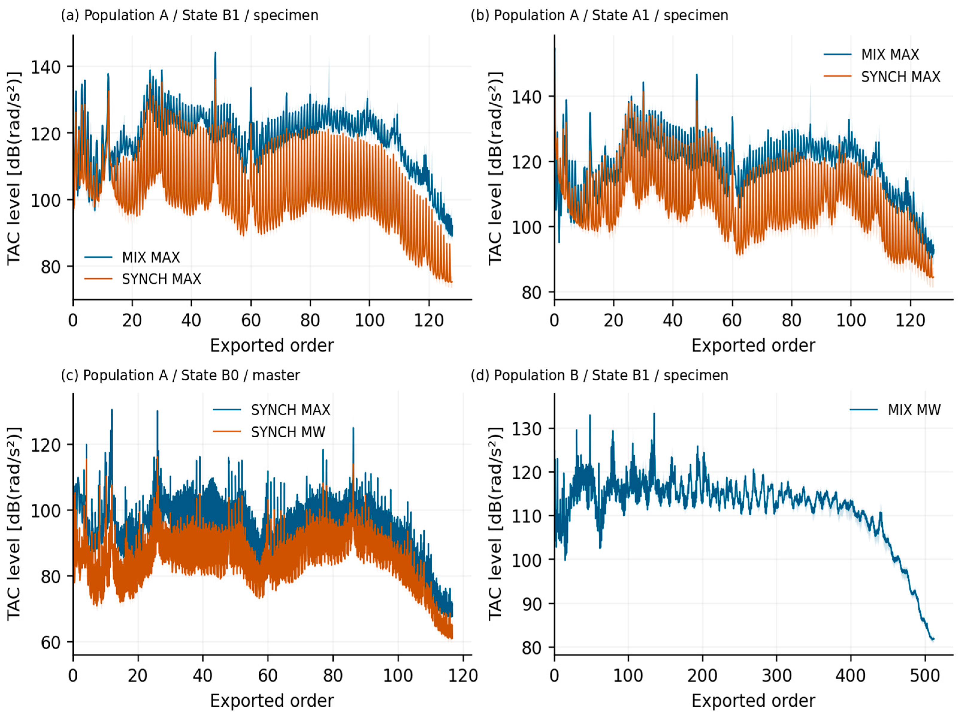
MAX and MW distinguish export variants. MW is conventionally associated with a mean-labeled export, but the precise averaging domain, amplitude or power averaging rule, and order of operations must be confirmed. Likewise, SYNCH is a synchronous-labeled output; its reference shaft and averaging implementation have not been established. Different native coordinate spacings must not be taken as sufficient evidence of a shaft-speed ratio. Figure 2 shows population median spectra and interquartile intervals without converting or interpolating the original axes. Section 3.5 reports complementary dispersion statistics for four representative specimen channels.
The Population A specimen MIX spectra contain 1024 coordinates from order 0 to 127.875 in increments of 0.125. Their SYNCH counterparts contain 512 coordinates from order 0 to 127.75 in increments of 0.25. The Population A master spectra contain 2048 coordinates ending at approximately 116.715, with an increment of approximately 0.0570175. The Population B MIX spectrum contains 2048 coordinates from order 0 to 511.75 in increments of 0.25. The exact numerical column labels remain authoritative, particularly for the master grid, whose exported decimal coordinates can show rounding in individual increments.
The observed TAC annotation is dB(rad/s2), whereas response B is labeled dB(m/s). These labels are preserved as exported. The reference quantity underlying each logarithmic scale, the relevant amplitude or power convention, and the derivation of response B from the measurement chain have not been supplied. Consequently, absolute linear amplitudes are not reconstructed, and the two quantities are not pooled into a common response. A difference between values on a consistently defined logarithmic channel remains a numerical contrast on that channel, but comparisons across physical quantities require a documented calibration and transformation.

2.3. Quality Assessment and Channel Relationships

All Population A files in the core have complete event identifiers. Each Population A specimen export contains 5733 redundant rows when comparison excludes the sparse ord annotation. Removing these repeated export rows leaves 55,317 distinct State B1 events or 55,316 distinct State A1 events. The difference is one additional State B1 event; exact joining yields 55,316 common State A1–State B1 events. These counts describe export structure, not repeatability of the mechanical measurement.
The Population B export has 56,398 rows and no redundant rows under the same rule. However, 42 rows lack serial_number. They are retained in the raw inventory and excluded from component counts, first-observed summaries, paired joins, and repeat-test calculations. The remaining 56,356 complete-key events correspond to 54,396 components with complete pseudonymous identifiers. Treating a missing identifier as one shared component would both inflate the component count and create an artificial repeated-measurement group.
Only one nonfinite spectral ordinate was found: in the State A1 SYNCH TAC MAX export at order 127.75. It is treated as missing for numerical summaries, with the rest of the affected spectrum retained. Its location lies outside the bearing-order windows considered below. This isolated missing value does not justify interpolation across the full dataset or deletion of all observations in the affected channel. The released inventory records its location and the number of nonfinite values per file.
Table 3 summarizes exact event-level joins. The join key comprises time, serial_number, type, and test_bench. Each side must be unique on this complete key after redundant rows are removed; a many-to-many join is an error. The 15,112 State B0 master events match the corresponding State B1 specimen subset, equivalent to approximately 27.3% of the State B1 events. The two State B0 master variants match all 15,112 events. These relationships make paired processing comparisons possible, while the early termination of master coverage limits their temporal generalization.

2.4. Operational Repeat Tests

After redundant export rows are removed, the Population A State B1 channel contains 351 components with more than one event, representing approximately 0.639% of its 54,920 components and 397 additional events. Comparing the first and last accessible results for these components gives 149 transitions from n.OK to OK and 202 from OK to OK. The result field represents the operational inspection outcome. Neither an initial n.OK nor a later OK is a verified bearing-condition diagnosis.
These observations are selected operational retests, rather than a balanced repeatability and reproducibility experiment. A retest may follow an intervention, a changed fixture state, or an inspection decision that is not recorded in the spectrum export. The observed first-to-last changes therefore cannot identify the rig’s intrinsic measurement uncertainty. They also cannot establish that cleaning caused a spectral change. Separating measurement variance from manufacturing or assembly variance requires additional experimental information and a suitable repeated-measures design.
The revised selection-bias analysis confirms that the retest subset is strongly outcome-selected. Among the 351 retested components, 149 (42.45%) had an initial n.OK result, whereas only four of the 54,569 non-retested components (0.0073%) had an initial n.OK result. Equivalently, 149 of 153 components with an initial n.OK result (97.39%) were retested, compared with 202 of 54,767 components with an initial OK result (0.369%). Of the retested components, 330 had two events, and 21 had three to seven events. The median first-to-last interval was 18,154 s (5.04 h), with an interquartile range of 6957–84,368.5 s (1.93–23.44 h). These figures demonstrate substantial operational selection and further exclude interpretation of this subset as an unbiased bench repeatability sample. This selection mechanism also limits unbiased longitudinal inference from within-component changes unless the retest process itself is explicitly modeled.

3. Methods

3.1. Reproducible Data Preparation

The companion workflow uses Python 3.12, pandas 2.2.3 [9], NumPy 2.3.5 [10], and PyArrow 25.0.1 [11]. It processes each file separately, preserving the numerical axis and retaining metadata needed for linkage. Package versions, file checksums, and the exact core-file selection are recorded. The code first reads the schema and converts only the spectral column names to floating-point coordinates. It verifies strictly increasing coordinates, counts missing metadata and nonfinite spectral values, and checks the observed grid extent.
To make the revised analyses directly inspectable, Supplementary File S1 provides the executable Python workflow used for the expanded grid, threshold/voting, reference-ratio, outlier, retest-selection, and temporal-selection checks. Supplementary File S1 also contains the resulting aggregate CSV tables and Figures S1 and S2. A separate leakage-aware example demonstrates GroupShuffleSplit and GroupKFold with a component grouping key constructed from pseudonymous type and serial_number so that all representations and repeat tests of one component remain in a single validation partition.
Redundant exports are identified by row hashes computed over all columns except ord. After retaining one representative, the complete event key must be unique. This check prevents conflicting records with the same complete key from silently entering downstream joins. The count of removed rows is reported separately from the count of subsequent measurements of a component. Rows with incomplete keys remain part of the source inventory but are excluded from analyses requiring traceability. No operational outcome category is removed from the primary cohort.
For descriptive population curves, complete-key events are sorted by time and the earliest event for each serial_number–type pair is selected within a channel. The median and the 25th and 75th percentiles are calculated independently at every original spectral coordinate using finite values. Thus, the displayed interquartile interval represents cross-component dispersion at a coordinate. It is not a confidence interval for the median, a spectrum of a median physical component, or an estimate of measurement uncertainty. Daily plots use the same first-observed selection and calendar dates derived from the stored timestamps.
Paired comparisons are constructed by an exact one-to-one join on the complete event key. The earliest common event per serial_number–type pair is then retained. This order of operations ensures that both values in a contrast belong to the same event. Selecting an arbitrary first row independently from unmatched channel subsets could instead compare different inspections. The paired difference is computed for every retained component before its median is taken; a difference between two marginal medians is not substituted for that statistic.

3.2. Bearing Factors and the Order-Reference Assumption

A private bearing-reference calculation supplied for the study provides the dimensionless characteristic factors listed in Table 4. These factors parameterize an illustrative search in the spectra. General interpretation of bearing-related periodicities follows established vibration-diagnostic principles [12]. The private reference does not, by itself, establish the bearing location in the rig or its rotation relative to each exported order reference. The source filename, component designation, and application-specific installation details are intentionally omitted from the public manuscript.
The characteristic factors were not fitted to, or inferred from, the released spectra. They were supplied as outputs of a private bearing-reference calculation associated with the industrial study. Because the underlying geometry, bearing designation, and source document are not released, the factors should be treated by public users as fixed, de-identified numerical inputs to the sensitivity analysis rather than as independently verifiable bearing geometry.
A bearing frequency factor becomes a spectral order only after its rotational reference is mapped to the reference used by the spectrum. Equation (1) states the required relation for a factor defined with respect to a bearing rotational rate.
o b = k b   ·   n b n r e f
Here, kb is the dimensionless factor, nb is the applicable bearing rotational rate, and nref is the rotational rate defining order one in the exported spectrum. The two rates must use consistent units. For configurations with both rings rotating, the factor definition and relative motions require explicit treatment. The direct search used below sets nb/nref to one as a sensitivity-analysis assumption. It is not a verified kinematic assignment for the industrial test rig. In particular, no speed ratio is derived from the ratio of the native spectral grid spacings.
The original bearing-reference document is not included in the public repository. To protect industrial context, the public manuscript reports only the de-identified characteristic factors required to reproduce the illustrative grid-sensitivity analysis; the private source filename, component designation, and application-specific details are omitted.
Because the actual rotational mapping is unavailable, an additional normalized reference-ratio sensitivity study varies r = nb/nref from 0.5 to 2.0 in increments of 0.1 for the Population A State B1 MIX TAC MAX native grid at w = 0.125. This range is used only to demonstrate dependence of the numerical indicator on the unknown mapping; it is not presented as a physically verified or application-specific transmission-ratio interval.

3.3. Local Prominence and Grid Sensitivity

For each of the BPFO, BPFI, BSF, and RPFFB families, the first three harmonic targets are evaluated under the direct-reference assumption. Around each target, the local peak is the largest finite exported value inside a symmetric search window of halfwidth w. The local background is the median of finite coordinates lying between 0.5 and 1.0 order away from that target on either side. Equation (2) defines the resulting logarithmic prominence.
P i h = m a x x   ∈   W h   L i ( x ) − m e d i a n x   ∈   B h   L i ( x )
In Equation (2), x is an exported order coordinate, Li(x) is the logarithmic spectrum for component i, and h is the harmonic index. The set Wh contains coordinates within w of the target h × ob; Bh contains coordinates between 0.5 and 1.0 order away from the same target. The peak and background sets are defined explicitly in the analysis code; empty sets are rejected. The family score in Equation (3) is the median of the three harmonic prominences. An illustrative flag is assigned when at least two of the three prominences reach 6 dB. This criterion is a transparent numerical example, not a validated industrial acceptance threshold.
S i = m e d i a n h   ∈   { 1 ,   2 ,   3 }   P i h
The sensitivity analysis evaluates halfwidths of 0.125 and 0.25 order. It also compares the native Population A MIX axis against its subset of coordinates shared with the 0.25-order SYNCH axis. For MIX data, the latter operation retains every second native coordinate. It does not re-estimate a spectrum, conserve spectral energy through a defined resampling filter, or equalize the physical resolution and windowing of two acquisition chains. The term shared coordinates refers only to where already exported values are evaluated.
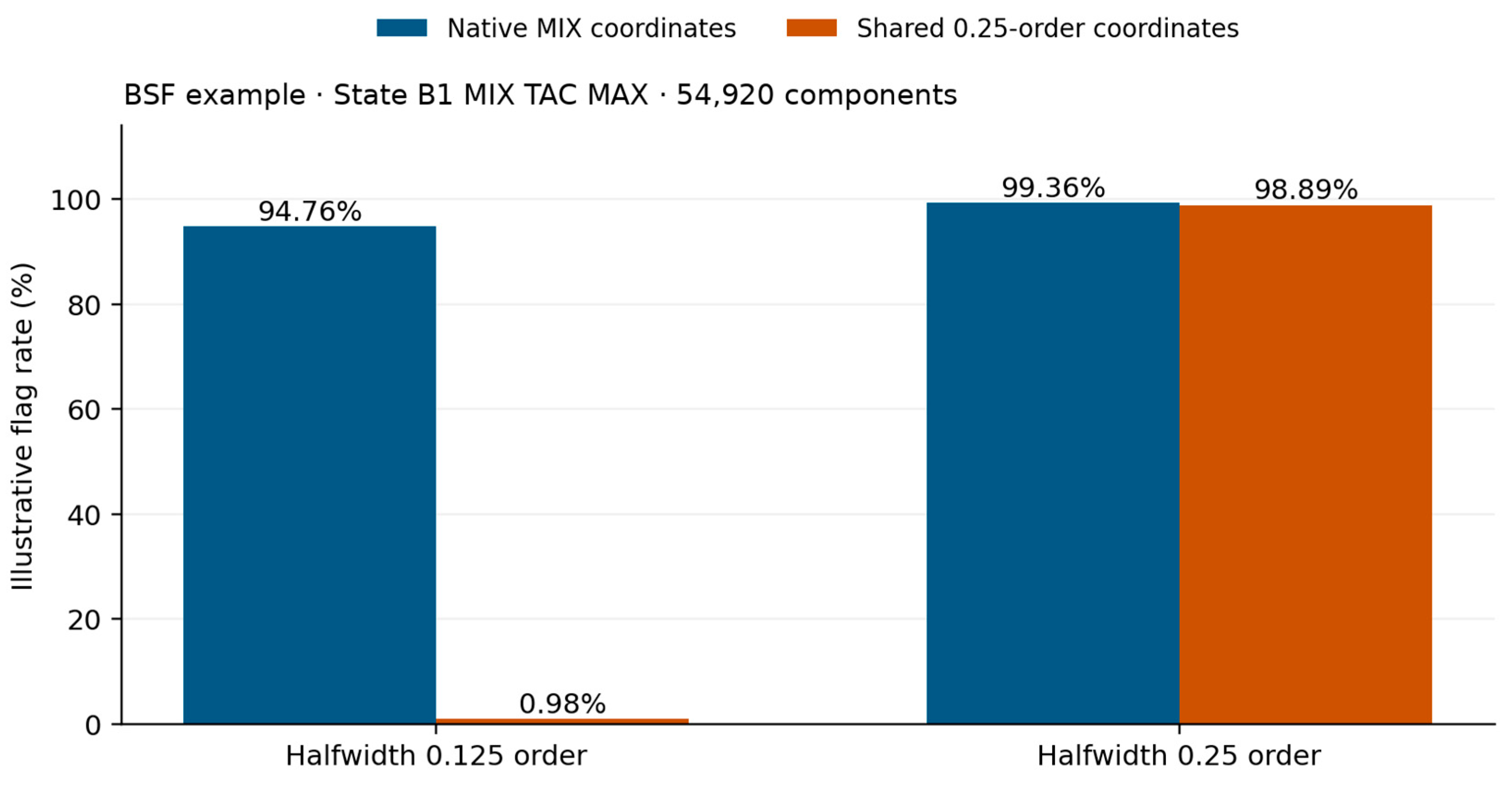
Figure 3 illustrates the consequences for the BSF example in the State B1 MIX TAC MAX channel. Among 54,920 first-observed components, the flag rate is 94.76% on the native axis with w = 0.125, but 0.98% after restriction to shared coordinates. With w = 0.25, the corresponding rates are 99.36% and 98.89%. The large narrow-window change demonstrates that coordinate selection can dominate this indicator. It cannot be interpreted as a change in the physical bearing population, which is identical in all four calculations.
The revised analysis extends the native-versus-shared-coordinate check to all four bearing families and all four Population A MIX TAC specimen representations. Under the original 6 dB, two-of-three-harmonics rule with w = 0.125, State B1 MAX native/shared flag rates were 0.025/0.000% for BPFO, 1.113/0.0036% for BPFI, 94.763/0.981% for BSF, and 23.314/1.020% for RPFFB. The magnitude of the grid effect was not universal: the BSF rate was 99.731/96.256% in State A1 MAX, 99.938/99.898% in State B1 MW, and 11.832/11.901% in State A1 MW. The complete family × representation × window × grid matrix is supplied in Supplementary File S1. These results show that coordinate restriction can have negligible, moderate, or extreme effects depending on the family and export representation.
Threshold and harmonic-voting sensitivity were also evaluated. In State B1 MAX on the native grid with w = 0.125 and a two-of-three rule, BSF flag rates were 99.925%, 94.763%, 40.572%, and 3.212% at thresholds of 3, 6, 9, and 12 dB, respectively; the corresponding RPFFB rates were 60.768%, 23.314%, 5.683%, and 0.208%. BPFI changed from 16.721% at 3 dB to 1.113% at 6 dB and 0.007% at 9 dB, while BPFO changed from 5.528% to 0.025% and then 0%. At 6 dB, changing the voting rule from one-of-three to two-of-three to three-of-three changed BSF from 99.996% to 94.763% to 0% and RPFFB from 99.712% to 23.314% to 0.193%. The 6 dB two-of-three rule is therefore retained only as an illustrative example rather than a validated diagnostic criterion; its practical diagnostic relevance has not been established. The complete threshold-sensitivity summary is provided in Supplementary Figure S2.
The normalized reference-ratio sweep provides a second sensitivity check on the unverified direct-reference assumption. Across r = 0.5–2.0 on the State B1 MAX native grid at w = 0.125, the illustrative two-of-three 6 dB flag rate ranged from 0.004% to 60.062% for BPFO, 0.007% to 97.937% for BPFI, 0% to 94.763% for BSF, and 0% to 97.383% for RPFFB. The non-monotonic changes arise because moving the assumed target orders samples different structures in the exported spectrum. Consequently, the r = 1 results cannot be interpreted as bearing-condition prevalence or as evidence that the bearing rotational rate equals the exported order reference. The normalized ratio sensitivity curves are provided in Supplementary Figure S1.

3.4. Paired Examples and Interpretive Limits

Table 5 reports median paired BSF prominence differences under the direct-reference assumption, using native coordinates and w = 0.125. The MIX-minus-SYNCH contrasts are positive for all four available Population A specimen pairs. Their magnitudes depend on the operating code and export variant. These comparisons document how the chosen indicator behaves across paired exports; they do not isolate a synchronous or nonsynchronous physical source.
The State B0 master MAX-minus-MW prominence contrast is negative, despite the export labels. A local prominence is a peak relative to its own background. It need not preserve the ordering of absolute peak levels when both the peak and the background change between processing variants. Consequently, the sign of a prominence difference alone should not be used to infer amplification or attenuation of a bearing excitation. The same reasoning applies to interpreting a mixed-minus-synchronous score as a direct estimate of a bearing-related contribution.
The illustrative results are descriptive. There is no verified bearing-fault label, calibrated contamination severity, or intervention record against which to validate a diagnostic classifier. No sensitivity, specificity, or predictive accuracy for bearing faults is claimed. Similarly, the exported spectra and sparse operational retests do not support subtracting a known rig uncertainty from the population spread. More detailed acquisition metadata would allow additional analyses, but cannot be reconstructed reliably from the Parquet filenames.

3.5. Component-to-Component Spectral Variability

Four channels are analyzed: Population A State B1 mixed maximum and synchronous maximum, Population A State A1 mixed maximum, and Population B State B1 mixed mean (Table 1, IDs 15, 13, 02, and 16). Redundant rows are identified from all columns except ord, with exact equality checks for repeated hashes. Rows missing any field of the event key (time, serial_number, type, test_bench) are excluded. Within each channel, the earliest event with a complete key and at least one finite ordinate is retained per serial_number–type pair, irrespective of operational outcome. No finite extreme is trimmed. The cohorts contain 54,920 components per Population A channel and 54,396 Population B components after excluding its 42 incomplete identifiers. Every selected ordinate is finite; N therefore equals the component count at every coordinate.
Each native coordinate is summarized by N, arithmetic mean, sample SD (denominator N − 1 ), minimum, maximum, min–max span, median, Q25, Q75, IQR ( Q 75 − Q 25 ), P5, P95, and P95–P5 span. These statistics use exported logarithmic TAC values; the mean is an arithmetic mean of dB values, not a linear-amplitude or energy mean. Dispersion is expressed in dB. Quantiles use linear interpolation between sorted observations at zero-based index ( N − 1 ) p for probability p; spectral coordinates are not interpolated. Table 6 then reports median SD, P90 SD, and median spans across each channel’s own native coordinates, including order zero, with equal coordinate weights. These summaries are not integrated spectral levels or controlled cross-channel comparisons: the native grids and their extents differ.
The arithmetic mean is used only as a descriptive location statistic across already exported logarithmic values. It is not a vibration-energy average or an integrated level. Likewise, the MW representation is a source-provided mean-labeled export and is not generated by the present analysis; its undocumented internal averaging operation must not be conflated with the cross-component arithmetic statistics reported here.
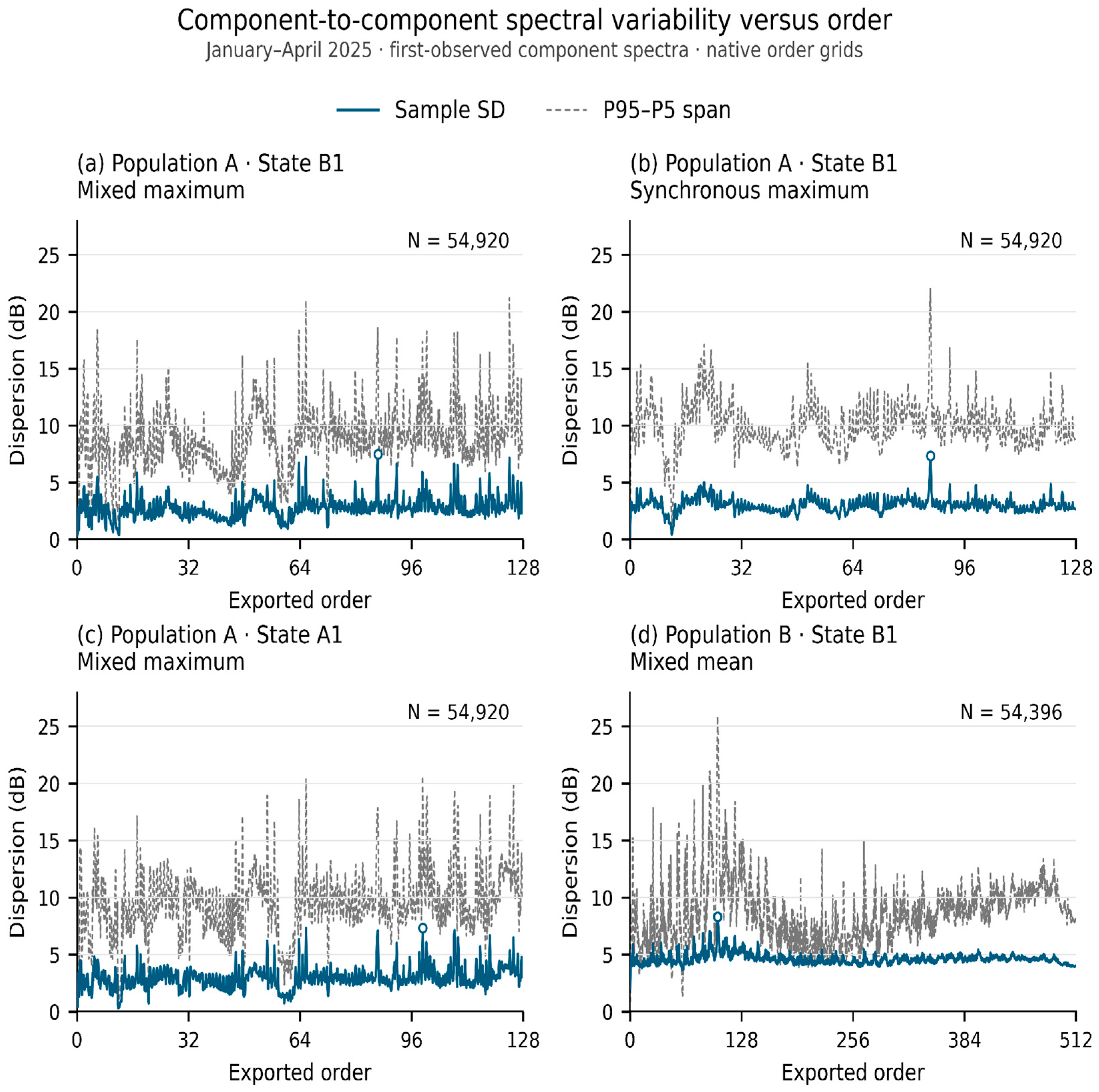
The three Population A channels have median SDs of 2.67–2.90 dB, median IQRs of 3.61–3.96 dB, and median P95–P5 spans of 8.75–9.65 dB. Population B combines a higher median SD (4.57 dB) with a smaller median IQR (2.47 dB) and a median P95–P5 span of 8.61 dB. This different ordering demonstrates the need to report several dispersion measures. Figure 4 displays SD and P95–P5 on each native grid.
The largest individual SDs in the two Population A State B1 channels occur near order 86: 7.48 dB at order 86.375 in the mixed maximum and 7.35 dB at order 86.25 in the synchronous maximum. The mixed channel also has pronounced dispersion at orders 65.75 and 124.125, the latter yielding its largest P95–P5 span of 21.21 dB. In State A1 mixed maximum, both the SD maximum (7.35 dB) and P95–P5 maximum (20.63 dB) occur at order 99.25, with additional SD peaks at 65.75 and 108.375. These isolated peak locations differ from a broad-band summary: among the descriptive intervals 0–8, 8–16, 16–32, 32–64, 64–96, and 96–128 (lower bound included, upper bound excluded), the State A1 mixed channel has its largest band-median SD in 96–128 (3.18 dB), while the State B1 mixed channel has similar largest band medians in 64–96 and 96–128 (both 2.83 dB). The State B1 synchronous channel has its largest band median in 16–32 (3.34 dB), despite its sharp single-coordinate maximum near 86. These intervals summarize already computed statistics; they do not redefine the spectral coordinates.
Population B shows its strongest local dispersion around orders 100–102. Both its maximum SD (8.33 dB) and maximum P95–P5 span (25.90 dB) occur at order 100.5. Its band-median SD is 5.28 dB in 96–128, compared with 4.53, 4.53, and 4.60 dB in the wider intervals 128–256, 256–384, and 384–512, respectively. Thus, the strongest local feature is concentrated near 100–102 even though variability remains present throughout the wider exported range. These order locations identify where the observed spectra differ most strongly; assigning them to specific geometry, bearing families, or excitation mechanisms would require the missing kinematic and acquisition metadata.
The full min–max span requires separate interpretation. In Population B it reaches 205.89 dB at order 42, where the exported minimum and maximum are −51.26 and 154.63 dB(rad/s2), respectively. At that same coordinate, SD is 4.50 dB, IQR is 2.89 dB, and the P95–P5 span is 7.04 dB. Only 26 of the 54,396 selected values (0.048%) lie below zero on the exported logarithmic scale. The large range is therefore strongly influenced by sparse tail observations and should not be presented as the typical difference between components. Their physical or operational origin cannot be established from the exports, so these finite observations are retained rather than silently removed. SD describes overall dispersion and uses more information than the two extremes, but remains sensitive to outliers. IQR and P95–P5 provide more resistant descriptions of the central 50% and 90% of the observed values. Their intervals need not imply a Gaussian distribution, and the full range remains useful for documenting extremes.
Additional robust diagnostics confirm that the 205.89 dB full range is dominated by a small operationally concentrated tail. At order 42, the cohort median is 120.817 dB, and the median absolute deviation is 1.4455 dB (scaled MAD 2.1431 dB). A three-IQR rule identifies 127 observations (0.2335% of the cohort); 50 of these 127 observations (39.37%) have n.OK status, compared with an overall n.OK rate of 0.974%. All 26 negative order-42 values are n.OK observations and occur on two stored measurement dates. The most negative observation is not an isolated single-coordinate excursion: values between orders 40 and 44 remain near the same low level. The maximum observation is also accompanied by elevated neighboring values. These patterns argue against treating the 205.89 dB span as typical component variability or as a single-cell numerical artifact, but the exports do not identify whether the tail reflects a measurement-chain state, an operational rejection condition, or another physical/process cause. The finite values are therefore retained and reported transparently. Distinguishing among these possibilities would require synchronized acquisition-chain, fixture, and operating metadata that are not available in the public release.
The appropriate interpretation is an observed component-to-component variability under production rolling-test conditions. The test bench’s independent repeatability and reproducibility uncertainty has not been determined. Consequently, manufacturing and geometric variability cannot be fully separated from measurement, fixturing, and operating contributions. Selecting one event per component prevents operational retests from overweighting the population, but does not remove those contributions or establish a causal variance decomposition. No bench uncertainty is subtracted from these SDs, and none of the reported spans are claimed to measure manufacturing variability alone.

4. User Notes

4.1. Recommended Reuse and Validation Splits

The collection supports descriptive spectral analysis, comparison of processing representations, study of temporal coverage, and development of data-handling methods for industrial condition monitoring. Models can also be explored against operational outcomes if that prediction target is explicitly defined. Such work should report the category frequencies and clarify that operational rejection can have causes beyond a bearing defect. The public data do not include a rejection-cause taxonomy. Therefore n.OK should be treated as a broad operational outcome and must not be mapped retrospectively to a localized bearing-race defect, gear-mesh anomaly, fixture resonance, slippage, or any other specific mechanism without independent labels. Likewise, the bearing characteristic factors reported in Table 4 should be treated as de-identified numerical inputs, not as publicly verified geometry. Before assigning physical meaning to bearing-related orders, users should independently establish the relevant bearing geometry, rotational mapping, and spectrum reference.
All representations and repeated events belonging to one component should remain in the same validation partition. Randomly dividing export rows risks placing redundant rows, different channels of the same event, or later inspections of a component in both training and test sets. This is a concrete instance of the broader leakage problem in scientific machine learning [13]. The recommended grouping variable is the validated component identity within its type. When temporal generalization is the objective, a chronological split should additionally prevent future data from informing feature selection, normalization, threshold fitting, or training. For comparisons across differing native order grids, users should preserve and report native-grid results and should not assume that interpolation, decimation, or restriction to common coordinates is diagnostically neutral. If a common grid is required, the transformation and a grid-sensitivity check should be reported together with the common-grid result.
Master-channel availability creates a second selection issue. The 15,112 matched master-covered State B1 events represent 27.319% of the 55,317 distinct State B1 specimen events and span 9 January to 13 February 2025; the 40,205 specimen-only events extend from 13 February to 17 April 2025. The operational n.OK rate is 0.668% in the master-covered subset and 0.192% in the specimen-only subset. On the 117 native coordinates used by the bearing-indicator analysis, the median absolute difference between the two subset medians is 0.85 dB, the 90th percentile is 2.36 dB, and the maximum is 9.49 dB. Under the original 6 dB, two-of-three, w = 0.125 native-grid rule, BSF flags occur in 89.68% of master-covered versus 96.62% of specimen-only events, while RPFFB flags occur in 15.12% versus 26.46%, respectively. These comparisons demonstrate measurable temporal selection and support reporting master-based results only for the early covered subset rather than generalizing them to the complete January-to-April population. The supplied metadata do not establish whether termination of master coverage reflects a planned protocol change, discontinuation of an export configuration, incomplete historical availability, or data loss, so no causal explanation is assigned.

4.2. Repository Contents and Metadata Limitations

The Zenodo Version 1.0 data package consists of the 13 anonymized Parquet files together with README.md, DATA_DICTIONARY.md, CITATION.cff, and SHA256SUMS.txt. The documentation defines the public schema and coordinate grids, describes the anonymization scope and reuse limitations, provides citation metadata, and records file-integrity checksums. No private source filenames, original component identifiers, or the private bearing-reference document are included in the public package.
Complete acquisition-chain metadata are not available in the exported tables. Sensor type and position, mounting arrangement, calibration and logarithmic reference quantities, sample rate, record duration, angular-resampling and spectral-windowing settings, speed and load conditions, reference shafts, and the precise engineering meanings of some export codes therefore cannot be reconstructed from the public Parquet files alone. The relation of the master representation to the specimen representation and the full definition of each operational outcome also remain incompletely documented. These limitations restrict absolute physical interpretation but do not prevent the file-level, event-level, component-variability, and grid-sensitivity analyses reported in this descriptor. No documented typical shaft-speed range in RPM or Hz and no detailed excitation-program description accompanied the released exports; these quantities are therefore not inferred from spectral grid spacing or file naming. The only defensible public context is that the files are derived spectra from component-level industrial rolling-test inspection. Reproducibility in this Data Descriptor consequently refers to reproducible processing and analysis of the released spectral exports, not reconstruction of the original acquisition chain from raw time histories. Accordingly, cross-study comparison of absolute order features or diagnostic thresholds should be undertaken only when the relevant acquisition and order-reference definitions are independently available.
In the public Parquet files, component identifiers, component-type identifiers, and test-bench identifiers are consistently pseudonymized while preserving within-dataset linkage. The stored time field is retained as chronology metadata; its timezone remains unconfirmed. The public tables do not contain explicit gear or bearing geometry, drawing numbers, CAD data, or direct manufacturing identifiers. Users should treat the pseudonymous identifiers and chronology fields as analytical metadata and should not interpret them as original industrial identifiers.

Supplementary Materials

The following supporting information can be downloaded at: https://www.mdpi.com/article/10.3390/data11100264/s1. Supplementary File S1, Supplementary Reproducibility Package, contains the executable analysis workflow, a leakage-aware grouped validation example, aggregate sensitivity and selection-bias CSV files, a README file, and Figures S1 and S2. The public dataset and repository documentation remain available through the Zenodo record specified above.

Funding

Supported by the EKÖP-26-3-I-SZE-17 University Research Fellowship Program of the Ministry of Science and Technology from the source of the National Research, Development and Innovation Fund.

Institutional Review Board Statement

Not applicable; the study concerns mechanical inspection data.

Informed Consent Statement

Not applicable.

Data Availability Statement

The anonymized industrial component rolling-test dataset described in this study [1] is publicly available in Zenodo at https://doi.org/10.5281/zenodo.22659642 (Version 1.0), under the Creative Commons Attribution 4.0 International (CC BY 4.0) license.

Acknowledgments

This research was carried out at the Vibro-Acoustics and Rotor Dynamics Research Group within the Audi Hungaria Faculty of Engineering at Széchenyi István University, Győr, Hungary. During the preparation and revision of this manuscript, the author used OpenAI ChatGPT (GPT-5.6 Sol; accessed on 8–29 September 2026) to assist with development and debugging of Python analysis code, preparation of candidate data-processing routines, document preparation, consistency checking, and language editing. All final data-selection rules, analytical parameters, executable code, numerical results, figures, interpretations, and manuscript statements were reviewed and verified by the author. AI-generated code or text was not treated as an independent source of scientific evidence, and the author takes full responsibility for the content of the publication.

Conflicts of Interest

The author declares no conflicts of interest.

Abbreviations

MIXMixed-labeled spectral representation retained from the source export; detailed proprietary processing semantics are not assigned.
SYNCHSynchronous-labeled spectral representation; exact reference shaft and averaging implementation are not established.
TACRetained response-channel label associated with exported values annotated as dB(rad/s2).
MAXMaximum-labeled export variant; detailed aggregation procedure is unavailable.
MWMean-labeled export variant; averaging domain, amplitude/power convention, and order of operations are unavailable.
BPFO/BPFFOOuter-ring bearing-pass/overrolling characteristic factor; BPFFO is the private-source label.
BPFI/BPFFIInner-ring bearing-pass/overrolling characteristic factor; BPFFI is the private-source label.
BSF/BSFFRolling-element spin/overrolling characteristic factor; BSFF is the private-source label.
RPFFBRing-pass factor on the rolling element, following the supplied bearing-reference terminology.
FTFRolling-element-set rotational factor for the stated ring-rotation case.
n.OKOperational rejection result; not a verified bearing-fault label.

References

  1. Horváth, K. Anonymized Production Rolling-Test Vibroacoustic Dataset for Bearing-Contamination Analysis in Automotive Drivetrain Components, Version 1.0. Zenodo. 2026. Available online: https://doi.org/10.5281/zenodo.22659642 (accessed on 10 September 2026).
  2. Wilkinson, M.D.; Dumontier, M.; Aalbersberg, I.J.; Appleton, G.; Axton, M.; Baak, A.; Blomberg, N.; Boiten, J.-W.; da Silva Santos, L.B.; Bourne, P.E.; et al. The FAIR Guiding Principles for scientific data management and stewardship. Sci. Data 2016, 3, 160018. [Google Scholar] [CrossRef] [Scilit] [PubMed]
  3. Smith, W.A.; Randall, R.B. Rolling element bearing diagnostics using the Case Western Reserve University data: A benchmark study. Mech. Syst. Signal Process. 2015, 64–65, 100–131. [Google Scholar] [CrossRef] [Scilit]
  4. Haneef, Z.; Umar, M.; Saleem, F.; Ullah, I.; Aqeel, K.; Siddique, M.F. Uncertainty-Calibrated Residual Conformal Monitoring of Wind Turbine SCADA Data for Cross-Asset Anomaly Detection Under Distribution Shift. Information 2026, 17, 930. [Google Scholar] [CrossRef] [Scilit]
  5. Siddique, M.F.; Bourezg, A.; Wisal, M.; Ali, S.; Umar, M.; Saleem, F.; Janjua, M.M. Bearing Fault Diagnosis: Class-Conditional Deep Domain Adaptation for Generalization Across Machines. In Proceedings of the 2026 International Conference on Robotics and Automation in Industry (ICRAI); IEEE: New York, NY, USA, 2026; pp. 1–7. [Google Scholar] [CrossRef] [Scilit]
  6. Fyfe, K.R.; Munck, E.D.S. Analysis of computed order tracking. Mech. Syst. Signal Process. 1997, 11, 187–205. [Google Scholar] [CrossRef] [Scilit]
  7. Wang, K.S.; Heyns, P.S. The combined use of order tracking techniques for enhanced Fourier analysis of order components. Mech. Syst. Signal Process. 2011, 25, 803–811. [Google Scholar] [CrossRef] [Scilit]
  8. Apache Software Foundation. Apache Parquet: Overview. Available online: https://parquet.apache.org/docs/overview/ (accessed on 8 September 2026).
  9. McKinney, W. Data Structures for Statistical Computing in Python. In Proceedings of the 9th Python in Science Conference, Austin, TX, USA, 28 June–3 July 2010; pp. 56–61. [Google Scholar] [CrossRef] [Scilit]
  10. Harris, C.R.; Millman, K.J.; van der Walt, S.J.; Gommers, R.; Virtanen, P.; Cournapeau, D.; Wieser, E.; Taylor, J.; Berg, S.; Smith, N.J.; et al. Array programming with NumPy. Nature 2020, 585, 357–362. [Google Scholar] [CrossRef] [Scilit] [PubMed]
  11. Apache Software Foundation. Apache Arrow Python (PyArrow) Documentation. Available online: https://arrow.apache.org/docs/python/ (accessed on 8 September 2026).
  12. Randall, R.B.; Antoni, J. Rolling element bearing diagnostics—A tutorial. Mech. Syst. Signal Process. 2011, 25, 485–520. [Google Scholar] [CrossRef] [Scilit]
  13. Kapoor, S.; Narayanan, A. Leakage and the reproducibility crisis in machine-learning-based science. Patterns 2023, 4, 100804. [Google Scholar] [CrossRef] [Scilit] [PubMed]
Figure 1. Daily first-observed component counts: (a) Population A State B1 specimen; (b) Population A State B0 master; (c) Population B State B1 specimen. Each component contributes once within a channel after redundant exports and incomplete keys are excluded. Zero counts denote no first observation in that channel on the stored date.
Data 11 00264 g001
Figure 2. Coordinate-wise median spectra (lines) and interquartile intervals (shading): (a) Population A State B1 MAX specimen exports; (b) Population A State A1 MAX specimen exports; (c) Population A State B0 master MAX and MW exports; (d) Population B State B1 MIX MW. Native axes are preserved. Different panels need not share the same physical order reference.
Data 11 00264 g002
Figure 3. BSF example in Population A State B1 MIX TAC MAX for the same 54,920 components. A flag requires at least two of three local harmonic prominences to reach 6 dB. Restricting exported values to shared coordinates changes the narrow-window flag rate markedly. The four rates are not estimates of bearing-fault prevalence.
Data 11 00264 g003
Figure 4. Component-to-component spectral variability versus order. Solid blue lines show sample SD; dashed gray lines show the P95–P5 span. Open circles mark each channel’s maximum SD. Panels (a–c) retain the Population A native grids (0.125, 0.25, and 0.125 order spacing); panel (d) retains the Population B grid (0.25 order spacing) and its wider extent. Line segments connect adjacent native coordinates within each channel only; no resampling, interpolation between grids, or smoothing is performed. The spans describe cross-component dispersion, not confidence intervals or bench measurement uncertainty.
Data 11 00264 g004
Table 1. Inventory of the validated 13-file core.
IDAnalytical RepresentationBinsExport RowsRedundant RowsComplete EventsComponents with Complete IDs
01Population A State A1 specimen SYNCH TAC MAX51261,049573355,31654,920
02Population A State A1 specimen MIX TAC MAX102461,049573355,31654,920
03Population A State B1 specimen SYNCH TAC MW51261,050573355,31754,920
04Population A State B1 specimen MIX TAC MW102461,050573355,31754,920
05Population A State A1 specimen MIX response B102461,049573355,31654,920
09Population A State A1 specimen SYNCH TAC MW51261,049573355,31654,920
10Population A State B0 master SYNCH TAC MW204815,112015,11214,962
11Population A State B0 master SYNCH TAC MAX204815,112015,11214,962
12Population A State A1 specimen MIX TAC MW102461,049573355,31654,920
13Population A State B1 specimen SYNCH TAC MAX51261,050573355,31754,920
14Population A State A0 master SYNCH TAC MAX204815,111015,11114,962
15Population A State B1 specimen MIX TAC MAX102461,050573355,31754,920
16Population B State B1 specimen MIX TAC MW204856,398056,35654,396
Counts are channel-specific and must not be summed as independent components. Population B has 42 incomplete identifiers; its complete-event and component counts exclude these rows. Redundancy is evaluated without the sparse ord annotation.
Table 2. Metadata and spectral-column dictionary.
FieldMeaning and Use
timeTimestamp of the exported measurement event; timezone unconfirmed.
serial_numberPseudonymous component identifier in the public release; 42 missing values in Population B.
typePseudonymous component-type code; retained in identity and event keys.
test_benchPseudonymous bench identifier; retained in the exact event key.
test_resultOperational result, including OK and n.OK; not a bearing-fault label.
groupSource grouping metadata; not used as a unique event identifier.
ordSparse physical-unit annotation; not the numerical axis.
numeric-named columnsSpectral ordinates at the order coordinates encoded in their column names.
Table 3. Exact event-level join coverage after redundancy removal.
Paired ChannelsLeft EventsRight EventsMatchedLeft Only
State B1 MAX: MIX/SYNCH55,31755,31755,3170
State A1 MAX: MIX/SYNCH55,31655,31655,3160
State B1 MW: MIX/SYNCH55,31755,31755,3170
State A1 MW: MIX/SYNCH55,31655,31655,3160
State B0 SYNCH: MAX/MW15,11215,11215,1120
State B1 specimen/State B0 master55,31715,11215,11240,205
State B1/State A1 MIX MAX55,31755,31655,3161
All listed right-side events have a left-side match. Key: time, serial_number, type, test_bench; one-to-one joins are enforced.
Table 4. De-identified bearing characteristic factors used in the illustrative order search.
Analysis LabelSource LabelSource MeaningFactor
BPFOBPFFOOuter-ring overrolling factor10.8085
BPFIBPFFIInner-ring overrolling factor12.1915
BSFBSFFRolling-element overrolling factor4.1424
RPFFBRPFFBRing-pass factor on rolling element8.2849
FTFiFTFFiRolling-element-set speed; inner ring rotating0.4699
FTFoFTFFoRolling-element-set speed; outer ring rotating0.5301
Source: private bearing-reference calculation supplied for the study. Conventional BPFO/BPFI/BSF abbreviations are mapped explicitly to the reference labels. The source filename, bearing designation, and application-specific installation details are not disclosed.
Table 5. Paired BSF prominence contrasts on native coordinates.
Left Minus Right ExportPaired ComponentsMedian Difference (dB)
State B1 MAX: MIX–SYNCH54,920+9.35
State A1 MAX: MIX–SYNCH54,920+11.81
State B1 MW: MIX–SYNCH54,920+9.82
State A1 MW: MIX–SYNCH54,920+3.99
State A1 MIX: MAX–MW54,920+7.23
State B0 SYNCH: MAX–MW14,962−12.31
Direct-reference assumption; first common event per component; three-harmonic median score; halfwidth 0.125 order. Values quantify local prominence differences, not isolated bearing-source amplitudes.
Table 6. Component-to-component spectral variability for four representative first-observed cohorts.
StatisticPopulation A
State B1
Mixed Maximum
Population A
State B1
Synchronous
Maximum
Population A
State A1
Mixed Maximum
Population B
State B1
Mixed Mean
Number of components54,92054,92054,92054,396
Native order coordinates102451210242048
Median SD (dB)2.672.902.904.57
P90 SD (dB)3.823.824.115.14
Maximum SD (dB)7.487.357.358.33
Order of maximum SD86.37586.2599.25100.5
Median IQR (dB)3.613.783.962.47
Median P95–P5 span (dB)8.759.659.498.61
Maximum P95–P5 span (dB)21.2122.0220.6325.90
Order of maximum P95–P5 span124.12586.2599.25100.5
Maximum min–max span (dB)51.0145.5942.78205.89
Order of maximum min–max span0.37598.87542
SD uses N − 1 . Quantiles are calculated from finite component values; medians and P90 in this table then summarize native coordinates. Orders are dimensionless exported coordinates. Values are rounded to two decimal places; peak locations retain native precision. No cross-grid interpolation or finite-outlier trimming is applied.
Disclaimer/Publisher’s Note: The statements, opinions and data contained in all publications are solely those of the individual author(s) and contributor(s) and not of MDPI and/or the editor(s). MDPI and/or the editor(s) disclaim responsibility for any injury to people or property resulting from any ideas, methods, instructions or products referred to in the content.