


Abstract
Burn wound instance segmentation on edge devices requires accurate contours and low inference cost. Light-YOLO-Seg replaces six bottlenecks in the YOLOv8n-Seg backbone with GhostV2 bottlenecks and adds coordinate attention at three feature fusion nodes while retaining the segmentation head. We split 455 original images at the image level into 364 training, 46 validation, and 45 internal test images before augmenting only the training set. On the internal test set, mask mean average precision at intersection-over-union thresholds of 0.50–0.95 (mAP50–95) reached 61.1%, up 5.4 percentage points over the baseline. Dice and mean boundary intersection over union reached 87.2% and 75.1%, respectively. Parameters and computational cost fell by 10.3% and 10.2%, respectively. Across five seeds, mask mAP50–95 was 61.21% ± 0.97%. On 80 cross-source images, it reached 53.6% versus 49.2% for the baseline. On a Raspberry Pi 5, mean inference latency and peak resident memory fell by 8.1% and 6.1%, respectively. The edge system displayed contours at 7.4 frames per second over 120 s using simulated silicone wounds. These results support lightweight wound segmentation and continuous contour display in the tested settings.
1. Introduction
Accurate delineation of visible burn wound contours facilitates local wound documentation, early observation, and the comparison of images captured at different time points. The Rule of Nines and the Rule of Palms are used to estimate the proportion of the burn area relative to the total body surface area, whereas image segmentation is employed to describe the boundaries and regions of individual visible wounds. Burn areas often exhibit uneven coloration, wound margins may gradually transition into the surrounding skin, and multiple spatially separated wounds may coexist within a single image. Manual delineation is susceptible to observer experience, illumination, and camera angles [1]. Portable red–green–blue (RGB) imaging devices facilitate pre-hospital and bedside image acquisition [2], endowing the automated extraction of wound contours with practical application value.
Existing studies on burn image analysis mostly concentrate on semantic segmentation. Xu et al. jointly segmented burn areas and body parts to assist on-site assessment [3], while BuRnSNet employed a two-way convolutional neural network to extract burn features [4]. Targeting pediatric burn images, Florea et al. investigated a data augmentation method that preserves scene information [5], and Li et al. proposed Pediatric BurnNet for multi-class segmentation and severity recognition [6]. These studies provide valuable methods for wound localization. However, when an image contains multiple wounds, the merged foreground mask cannot preserve the independent identity of each wound.
Binary semantic segmentation typically categorizes all wounds of the same class as foreground. To document individual wounds separately, additional steps such as connected component analysis must be incorporated to separate the regions. Adjacent wounds, unclear local boundaries, and elongated morphologies may lead to foreground adhesion or local segmentation omissions, rendering such separation unreliable. Burn char, dressings, and shadows further increase the difficulty of boundary identification. Therefore, in addition to region overlap metrics such as the Dice coefficient and Intersection over Union (IoU), instance detection and contour consistency should also be evaluated. Cassidy et al. fused information from multiple color spaces for chronic wound segmentation [7]. A review of skin lesion segmentation also identified morphological variations, noise, and imaging conditions as primary challenges [8]. These works provide references for color feature fusion and complex boundary representation.
Encoder–decoder architectures and multi-scale feature fusion are widely used in medical image segmentation, with representative models including U-Net [9], UNet++ [10], and DeepLabV3+ [11]. EGE-UNet reduces computational requirements through group enhancement [12], and PMFSNet utilizes multi-scale self-attention for feature fusion [13]. Boundary guidance has also been employed to improve contour errors [14]. GhostNetV2 enhances feature extraction efficiency through low-cost feature generation and decoupled fully connected (DFC) attention [15]. Coordinate Attention (CA) preserves positional information along the height and width directions [16]. More recent methods, including BDFormer [17], a lesion boundary detection model based on fusion of a convolutional neural network (CNN) and a Transformer [18], EM-Net [19], and SimpleUNet [20], focus on boundary representation, morphological features, or network simplification, respectively. Burn wound segmentation requires both low computational overhead and the preservation of narrow regions and weak boundary details; merely reducing network size may struggle to meet these dual requirements.
Burn image analysis is progressively being applied to portable devices. Yildiz et al. developed a mobile application for burn image segmentation and classification [21]; Xu et al. utilized smartphone RGB images for on-site assessment [3]; and Chang et al. compared light detection and ranging (LiDAR) with deep learning methods for two- and three-dimensional burn wound area measurement [22]. Light-M for resource-constrained environments [23] and knowledge distillation methods incorporating attention correction and boundary constraints [24] provide alternative approaches for lightweight medical segmentation. The parameter count and the computational cost in billions of floating-point operations (GFLOPs) reflect model size and theoretical computational demands, whereas actual performance also depends on image acquisition, post-processing, and display. Therefore, segmentation accuracy and continuous output capability on edge devices need to be evaluated separately.
Reviews on the evolution of You Only Look Once (YOLO) architectures and their medical applications [25,26] provide context for distinguishing model tasks and evaluation objectives. AS-YOLO uses Ghost bottlenecks in the backbone and a global attention mechanism in the neck for apple and stem segmentation [27]. YOLOv7-PSA targets burn severity detection [28], and ABC-YOLO investigates burn depth classification [29]. The specific problem addressed in this paper is reducing backbone computation while improving the segmentation of irregular contours under the condition of preserving an independent mask for each wound. To this end, GhostV2 containing a DFC branch is introduced into C2f, and CA is configured at the P3 fusion node of the feature pyramid network (FPN) and the P4 and P5 fusion nodes of the path aggregation network (PAN). This paper evaluates the accuracy and model size of this configuration in burn wound instance segmentation through module ablation, Ghost generational comparison, and CA placement comparison, and measures its operational performance on edge devices.
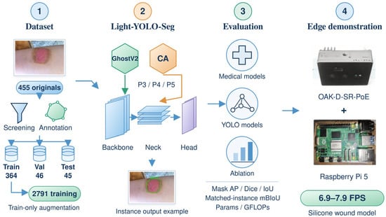
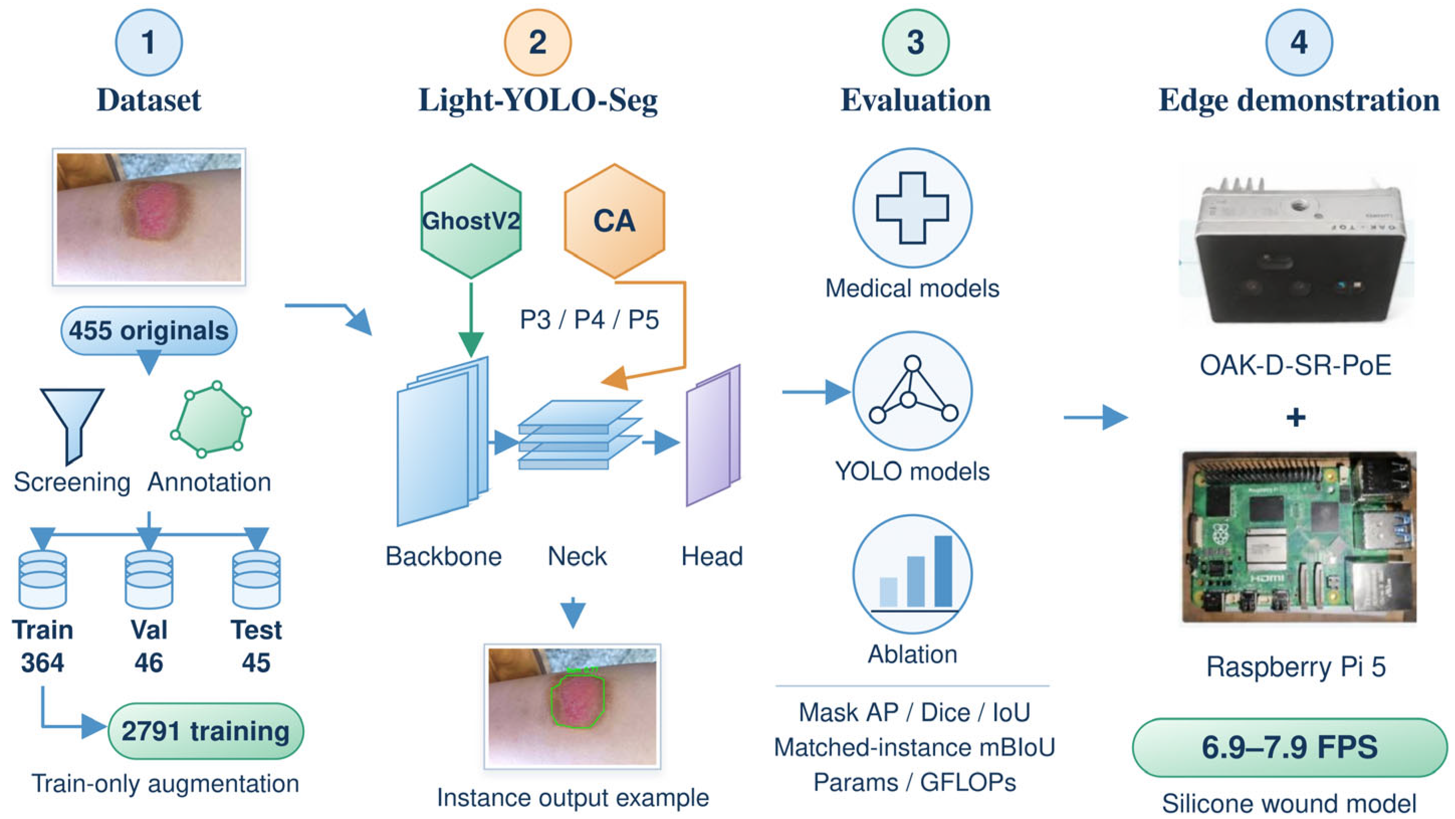
This study develops Light-YOLO-Seg based on YOLOv8n-Seg [30]. The backbone network retains the dual-branch aggregation structure of C2f and replaces six conventional bottleneck modules with GhostV2 bottleneck modules; CA is incorporated at the P3 fusion node of the FPN and the P4 and P5 fusion nodes of the PAN. The model retains the native instance segmentation head, outputting an independent mask for each wound. Using a unified data split, the model is compared with general medical segmentation methods, burn-specific methods, and YOLO instance segmentation models. Architectural modifications are evaluated through module ablation and CA placement ablation, and deployment performance is assessed on the Raspberry Pi 5 (Raspberry Pi Ltd., Cambridge, UK) and the OAK-D-SR-PoE (Luxonis Holding Corporation, Littleton, CO, USA). Figure 1 summarizes the research workflow.
Figure 1.
Research workflow and evaluation scope of Light-YOLO-Seg. CA = coordinate attention, YOLO = You Only Look Once, AP = average precision, IoU = intersection over union, mBIoU = mean boundary IoU, GFLOPs = billions of floating-point operations, and FPS = frames per second. Val = validation set, Params = parameter count, and PoE = power over Ethernet.
This study mainly includes the following three aspects:
- Replacing six conventional bottlenecks in the four C2f modules of the backbone network with GhostV2 bottlenecks while retaining the C2f aggregation method and the native segmentation head; incorporating CA after the concatenation of P3, P4, and P5 features to enhance positional information representation at different fusion scales.
- Evaluating region overlap, instance mask accuracy, boundary quality, and model complexity on the same test set; analyzing the combination of GhostV2 and CA, as well as the placement of CA at different fusion nodes, through ablation experiments.
- Implementing model conversion, RGB acquisition, Vision Processing Unit (VPU) inference, instance mask reconstruction, and contour display on the Raspberry Pi 5 and OAK-D-SR-PoE system, and measuring synchronous central processing unit (CPU) inference performance and system throughput in simulated wound scenarios, respectively.
2. Materials and Methods
2.1. Dataset Construction and Annotation
In this study, 455 original RGB burn wound images were collected and screened from publicly accessible web sources and clinical images provided by hospitals. Duplicate or highly similar images were first screened out, followed by selection based on image quality and wound contour visibility. The retained images covered various anatomical sites, wound morphologies, observation angles, and backgrounds.
The source records included 150 hospital images corresponding to 72 traceable patients and 305 publicly sourced images. In the split audit, the number of exact duplicate images across sets was 0; 6 groups of perceptual hash candidates were manually reviewed, and none were confirmed as near-duplicates across sets; and the traceable patient conflict across sets for the hospital-sourced subset was 0. Patient identity information for publicly sourced images was incomplete; therefore, the overall splitting unit was the image.
Two burn specialists used LabelMe 5.9.1 to perform polygon annotations on visible wounds. Spatially separated wounds within the same image were annotated as distinct instances, and the annotations were subsequently converted into an instance segmentation training format. When conducting semantic segmentation comparisons and evaluating region metrics, the instance masks within the same image were merged into a binary wound foreground; when conducting instance detection and boundary evaluations, the identity of each instance was retained.
Prior to offline augmentation, the 455 images were divided, using the original image as the unit, into a training set of 364 images, a validation set of 46 images, and an internal test set of 45 images. Offline augmentation was applied only to the training set, expanding it to 2791 training images, comprising 364 original training images and their augmented versions. The validation and internal test sets retained the original images. A total of 2882 images were used for training, validation, and internal testing.
Offline augmentation included random rotation at ±15° (probability 0.30), horizontal flipping (probability 0.50), brightness variation of ±20%, contrast variation of ±15%, and Gaussian noise with a standard deviation of σ = 8 (an 8-bit pixel scale). Additional online augmentation was disabled during training.
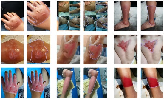
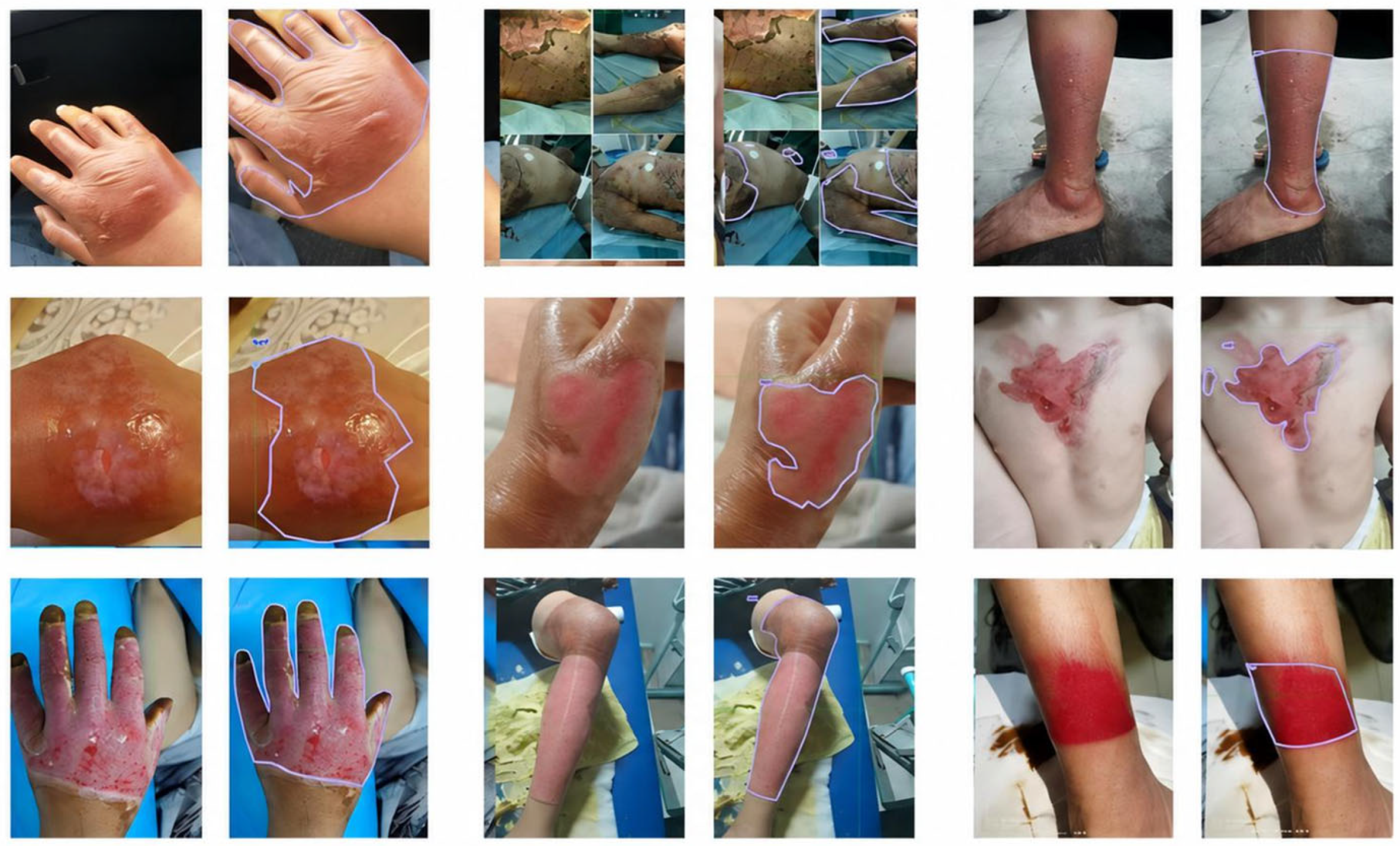
Representative images and annotations are shown in Figure 2, and the dataset composition is presented in Table 1. Model selection utilized the 46 original validation images, and the final performance was evaluated on the 45 original test images without offline augmentation.
Figure 2.
Representative red–green–blue (RGB) burn wound images and polygon annotations. Spatially separated wounds within the same image are annotated as distinct instances.
Table 1.
Dataset composition and usage.
2.2. YOLOv8n-Seg Baseline Model
This study selects YOLOv8n-Seg, which natively supports instance segmentation, to output separate results for multiple wounds within the same image [30]. The model directly predicts the bounding box, confidence score, and mask for each instance, reducing the reliance on connected component processing of binary foreground masks, and its nano-level architecture is also suitable as a foundation for adaptation to edge devices.
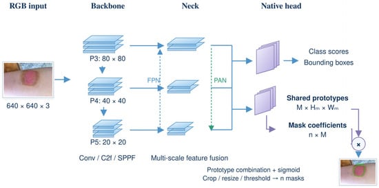
YOLOv8n-Seg consists of a backbone network, a neck network, and an instance segmentation head (Figure 3). The backbone network extracts multi-scale features through convolutions, C2f, and Spatial Pyramid Pooling-Fast (SPPF); the neck network combines FPN and PAN to achieve cross-scale feature fusion. The segmentation head constructs independent masks using shared mask prototypes and instance-specific coefficients. When the number of prototypes is M and the number of candidate instances is n, the prototype tensor dimension is M × Hm × Wm, and the coefficient tensor dimension is n × M; the combination of the two generates n instance masks.
Figure 3.
The functional architecture of YOLOv8n-Seg instance segmentation, including the backbone network, neck network, and native mask prediction head. Conv = convolution, FPN = feature pyramid network, PAN = path aggregation network, and SPPF = spatial pyramid pooling-fast.
This study retains the native segmentation head and concentrates modifications on the feature generation of the backbone network and the cross-scale feature fusion of the neck network.
2.3. Light-YOLO-Seg Architecture
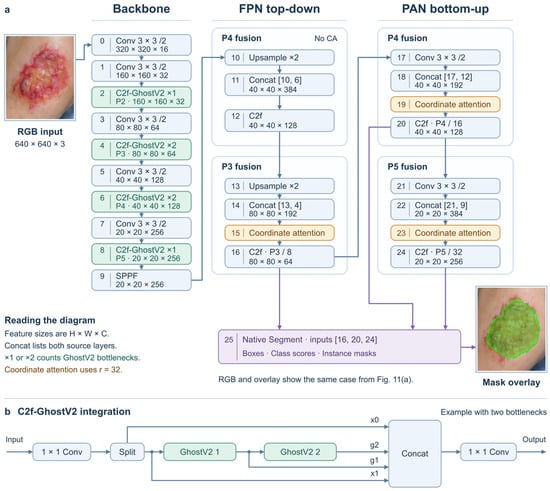
Light-YOLO-Seg retains the initial feature extraction layer, downsampling convolutions, SPPF, FPN/PAN, and the native Segment head of YOLOv8n-Seg. The input resolution is 640 × 640. Modifications are limited to the bottlenecks inside the C2f modules at layers 2, 4, 6, and 8 of the backbone network and three CA modules inserted after the Concat in the neck network and before the subsequent C2f. The layer indices below start from 0. Feature dimensions in the main text are represented as “height × width × channels”, while the CA formulas adopt “channels × height × width”.
2.3.1. Compressing the Backbone with C2f-GhostV2
The Ghost module first utilizes a small number of conventional convolutions to generate intrinsic features Y’, then generates additional features through low-cost transformations, and concatenates them along the channel dimension. Let s be the feature generation ratio including the intrinsic features, and φi denote the i-th additional transformation; the concatenation process is shown in Equation (1). In this study, s = 2 is set, meaning one set of intrinsic features and one set of features generated by 3 × 3 depthwise convolutions are used. GhostNetV2 further incorporates DFC attention to supplement spatial context [15].
The backbone network retains the initial feature extraction layer at layer 0, the downsampling convolutions at layers 1, 3, 5, and 7, and the SPPF at layer 9. The C2f modules at layers 2, 4, 6, and 8 are replaced with C2f-GhostV2, corresponding to P2/4, P3/8, P4/16, and P5/32, respectively, with the input and output channel numbers remaining unchanged. Their output dimensions are 160 × 160 × 32, 80 × 80 × 64, 40 × 40 × 128, and 20 × 20 × 256, respectively. Under the YOLOv8n depth coefficient of 0.33, the internal repetition counts are 1, 2, 2, 1, respectively, totaling 6 GhostV2 bottlenecks.
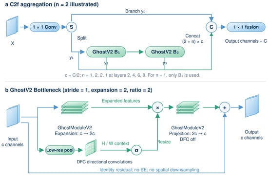
C2f-GhostV2 retains the dual-branch and progressive feature concatenation structure of the original C2f. The input is mapped by a 1 × 1 convolution and split into two groups of channels; one branch proceeds directly to the final concatenation, while the other passes sequentially through the internal bottlenecks. The output of each bottleneck is concatenated with the initial two branches and finally fused by a 1 × 1 convolution. The hidden channel ratio of C2f is 0.5, and the internal channel number c is 16, 32, 64, and 128, respectively. Each GhostV2 bottleneck first expands the channels to 2c, and then projects back to c.
The input and output channel numbers of each GhostV2 bottleneck are both c, with a stride of 1. In the expansion stage, GhostModuleV2 generates intrinsic features through a 1 × 1 conventional convolution and additional features through a 3 × 3 depthwise convolution, outputting 2c channels. The parallel DFC branch sequentially performs a 2 × 2 average pooling, a 1 × 1 convolution mapping channels from c to 2c, and 1 × 5 and 5 × 1 depthwise convolutions with 2c channels. Each convolution is followed by batch normalization, converting the attention features into weights via a sigmoid function; nearest-neighbor interpolation is used to restore spatial resolution, which is then element-wise multiplied with the main branch features.
The GhostModuleV2 in the projection stage does not use DFC; it projects the 2c channels back to c and adds them to the input via a residual connection. DFC is enabled in the expansion stage of all 6 bottlenecks. The Ghost feature generation ratio and channel expansion multiplier are both 2, and no additional Squeeze-and-Excitation (SE) module is used, nor is spatial downsampling performed; convolutions do not contain bias terms. ReLU is used in the expansion stage, and no activation function is used in the projection stage. Figure 4 illustrates the C2f feature aggregation and the internal structure of GhostV2.
Figure 4.
C2f-GhostV2 feature aggregation and the internal structure of the GhostV2 bottleneck. (a) C2f aggregation illustrated with two internal bottlenecks; (b) GhostV2 bottleneck with a stride of 1, an expansion multiplier of 2, and a Ghost feature generation ratio of 2. DFC = decoupled fully connected, SE = squeeze-and-excitation, and Concat = concatenation.
2.3.2. Enhancing Multi-Scale Features with Coordinate Attention
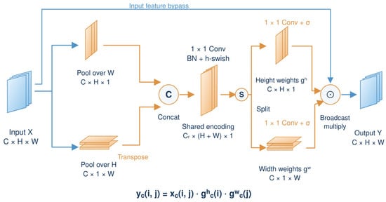
CA aggregates information along the height and width directions, respectively, preserving directional positional information during the channel re-weighting process [16]. The reduction ratio of the three CA modules is set to r = 32. For an input X with dimensions C × H × W, pooling along the width yields a height descriptor with dimensions C × H × 1, and pooling along the height yields a width descriptor with dimensions C × 1 × W. The descriptors corresponding to channel c are shown in Equations (2) and (3).
The width descriptor is transposed to C × W × 1 and concatenated with the height descriptor. After a shared 1 × 1 convolution, batch normalization, and h-swish activation, the intermediate feature f in Equation (4) is obtained. Here, F1 denotes the shared convolution, and δ denotes h-swish. The number of intermediate channels is Cr = max(8,⌊C/r⌋), with a minimum of 8. Therefore, inputs with 192, 192, and 384 channels yield 8, 8, and 12 intermediate channels, respectively.
The feature f is split along H and W, and the width descriptor is restored to its original orientation. Through independent 1 × 1 convolutions and the sigmoid function σ, the height weight gh and width weight gw in Equation (5) are generated. The weights are broadcast to the input dimensions and element-wise multiplied with X to obtain the output in Equation (6). CA does not change the number of channels or the spatial resolution (Figure 5).
Figure 5.
Coordinate Attention module, including independent height and width pooling, shared encoding, and directional feature re-weighting. BN = batch normalization and h-swish = hard swish.
The neck network retains the top-down FPN fusion and the bottom-up PAN fusion. Layer 10 upsamples the SPPF output, layer 11 concatenates it with the P4 features from layer 6 of the backbone network, and layer 12 (C2f) outputs a 40 × 40 × 128 feature. CA is not added at this initial P4 fusion node. The three selected nodes all follow the order of “Concat—CA re-weighting—original C2f”.
In the FPN path, layer 13 upsamples the feature from layer 12, and layer 14 concatenates it with the P3 features from layer 4 of the backbone network to generate an 80 × 80 × 192 feature. Layer 15 CA enhances it, and layer 16 C2f outputs the 80 × 80 × 64 P3/8 feature.
In the PAN path, layer 17 downsamples the feature from layer 16, and layer 18 concatenates it with the P4 feature from layer 12 to form a 40 × 40 × 192 feature. After layer 19 CA, layer 20 C2f outputs the 40 × 40 × 128 P4/16 feature. Layer 21 then downsamples this output, and layer 22 concatenates it with the SPPF output from layer 9 of the backbone network to form a 20 × 20 × 384 feature. Layer 23 CA enhances it, and layer 24 C2f outputs the 20 × 20 × 256 P5/32 feature.
Therefore, the number of input channels for the three CA modules is 192, 192, and 384; the subsequent C2f modules generate 64, 128, and 256 channel features, respectively, which are passed to the native segmentation head. CA is located after concatenation and maintains the feature dimensions unchanged, so the subsequent C2f continues to perform feature fusion.
2.3.3. Overall Network Architecture
Figure 6 shows the complete architecture. The four C2f-GhostV2 modules retain the scale and channel configuration of the backbone network, while the three CA modules enhance the fused P3, P4, and P5 features. After inserting CA, the input layer indices of the original Segment head change from [15, 18, 21] to [16, 20, 24]; Segment is layer 25 in the improved network. Its three input dimensions are 80 × 80 × 64, 40 × 40 × 128, and 20 × 20 × 256, corresponding to strides of 8, 16, and 32. Figure 6b illustrates the splitting, serialization, and progressive concatenation of GhostV2 within C2f, using two internal bottlenecks as an example.
Figure 6.
Light-YOLO-Seg network architecture and GhostV2 integration. (a) The four C2f-GhostV2 modules of the backbone network contain 1, 2, 2, and 1 GhostV2 bottlenecks, respectively. Three CA modules are located in the P3 of the FPN and the P4 and P5 of the PAN, after Concat and before C2f; the outputs of layers 16, 20, and 24 are fed into the native Segment head. Feature sizes are represented as height × width × channels. (b) Taking two bottlenecks as an example, one branch after the C2f split passes sequentially through two GhostV2 bottlenecks, and finally the two initial feature branches and the outputs of the two bottlenecks are concatenated and fused by a 1 × 1 convolution.
The native segmentation head predicts class scores, bounding boxes, shared mask prototypes, and instance-specific mask coefficients. The M × Hm × Wm prototype tensor is combined with the n × M coefficient tensor, followed by sigmoid activation, bounding box cropping, resizing, and thresholding to obtain n independent wound masks.
Keeping the segmentation head unchanged allows subsequent ablation experiments to separately evaluate the effects of backbone compression and fusion node enhancement.
2.4. Training Strategy and Loss Function
Light-YOLO-Seg is implemented in Ultralytics 8.3.0 and adopts the official yolov8n-seg.pt pre-trained weights, transfers weights for structurally matching layers, and re-initializes added modules. The input resolution is 640 × 640, with 200 training epochs and a batch size of 16. The stochastic gradient descent (SGD) optimizer is used with an initial learning rate of 0.01, momentum of 0.937, and weight decay of 0.0005. After 3 warm-up epochs, cosine annealing is applied with an end learning rate ratio of 0.01, targeting a final learning rate of 0.0001. The training employs the classification loss, bounding box regression loss, distribution focal loss, and instance mask loss of YOLOv8-Seg [30].
All comparison models share the same split of 364 original training images (2791 after offline augmentation), 46 validation images, and 45 internal test images. All models use 640 × 640 inputs and train for 200 epochs. Final weights are selected by the highest validation Dice. YOLO models use their official pre-trained weights and SGD with an initial learning rate of 0.01, momentum of 0.937, and weight decay of 0.0005. Other medical segmentation models follow their respective implementations for optimizer and pre-training settings. Region evaluation uses Dice and IoU for the binary wound foreground. Instance outputs are also evaluated by mask average precision (AP) and mean boundary intersection over union (mBIoU).
In a separate controlled run, YOLOv8n-Seg and Light-YOLO-Seg shared the data, SGD optimizer, learning rate, and random seed budget. Mask mean average precision over IoU thresholds of 0.50–0.95 (mAP50–95) was 55.9% and 61.4%, respectively, an increase of 5.5 percentage points, close to the 5.4 percentage point gain reported for the main comparison.
Controlled training and module ablation evaluate GhostV2 and CA.
2.5. Edge Deployment System
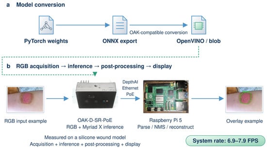
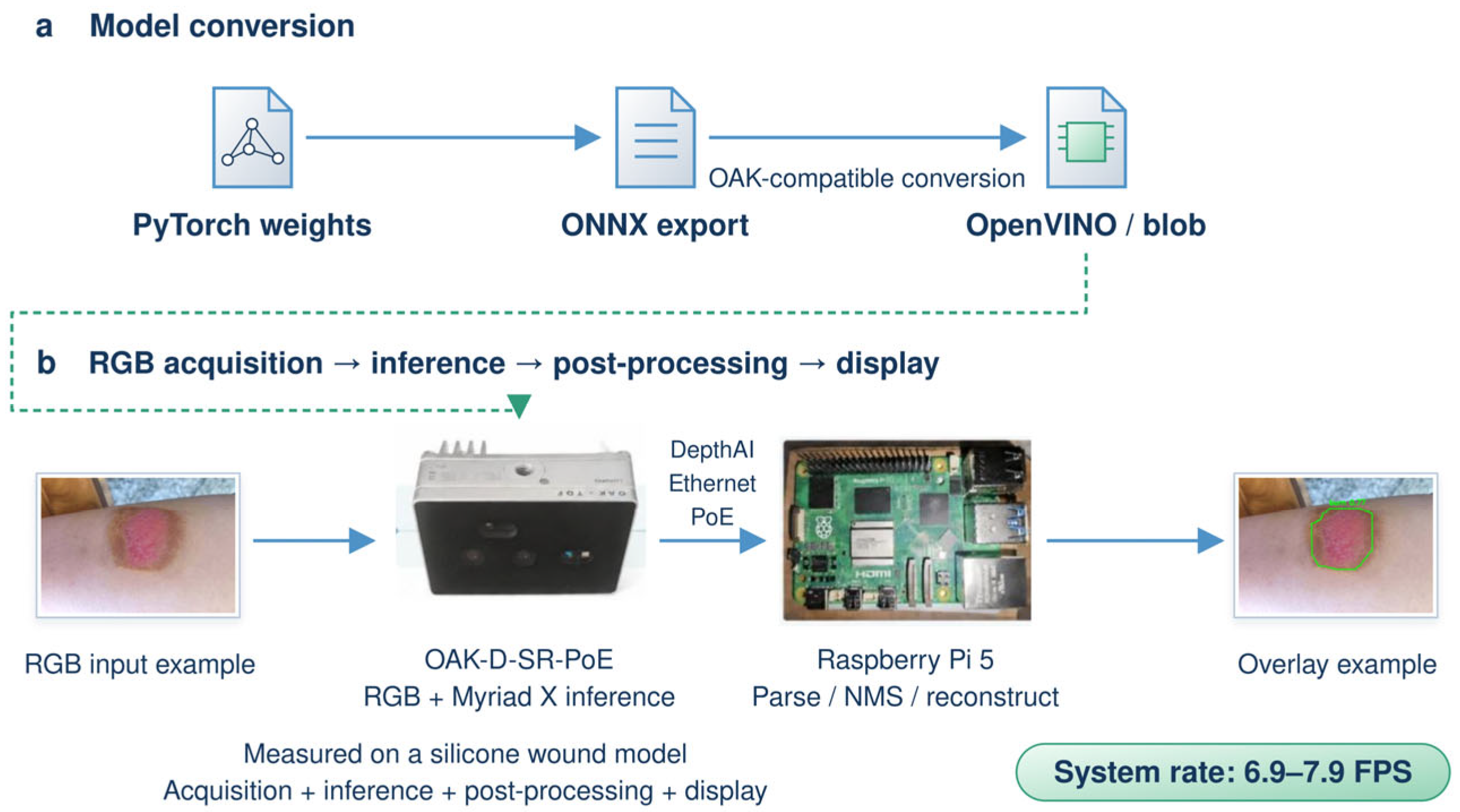
The OAK-D-SR-PoE captures RGB images and runs inference on its Myriad X VPU (Intel Corporation, Santa Clara, CA, USA). The Raspberry Pi 5 uses DepthAI 3.12.1 to stream data, parse predictions, rebuild instance masks, and display overlays. Figure 7 shows PyTorch 2.5.1 model export to Open Neural Network Exchange (ONNX) and conversion to OpenVINO 2022.3.0 and OAK-compatible blobs.
Figure 7.
Model conversion and edge deployment. (a) PyTorch to ONNX and OpenVINO/blob; (b) RGB capture, VPU inference, post-processing, and display on OAK-D-SR-PoE and Raspberry Pi 5. ONNX = Open Neural Network Exchange, CPU = central processing unit, NMS = non-maximum suppression, and VPU = vision processing unit.
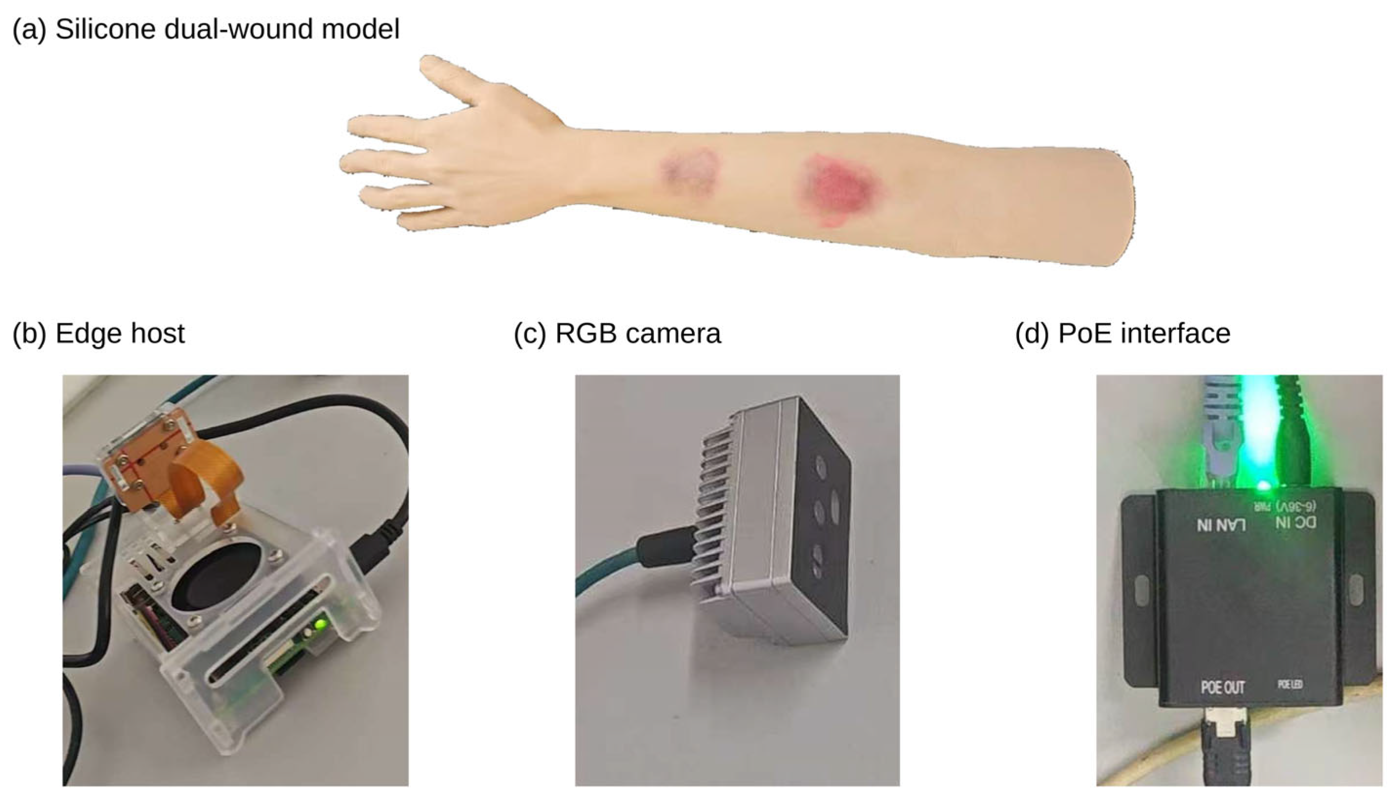
The Raspberry Pi 5 performs confidence filtering, Non-Maximum Suppression (NMS), mask coefficient and prototype combination, sigmoid transformation, resizing, and binarization, and displays the wound contours. The parameters are listed in Table 2. For online display, the matching of the same wound is determined by a mask IoU ≥ 0.50 between adjacent processed frames, and the contour is displayed after 3 consecutive confirmed frames. If a missed detection or matching failure occurs, the old contour of that wound is immediately removed and the count is reset to zero; upon re-detection, the 3 consecutive confirmation frames are required again. This rule is used only for online display. A silicone arm with two wounds was selected for the simulation demonstration, allowing changes in distance and camera angle on the same object to repeatedly check the complete workflow from camera acquisition and VPU inference to mask reconstruction and display. Real burn photographs were used for offline segmentation evaluation.
Table 2.
OAK acquisition and inference settings. NMS = non-maximum suppression, IoU = intersection over union, RGB = red, green, and blue, and FPS = frames per second.
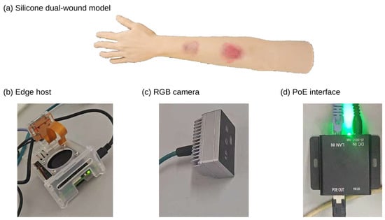
Figure 8 shows the silicone dual-wound model and the main components of the edge platform.
Figure 8.
Simulated wounds and platform components.
3. Experiments and Results
3.1. Experimental Environment and Training Settings
Offline training and testing were performed on an Intel Core i7 processor (Intel Corporation, Santa Clara, CA, USA) and an NVIDIA GeForce RTX 4060 Ti graphics processing unit (GPU, NVIDIA Corporation, Santa Clara, CA, USA) with 8 GB of video random-access memory (VRAM). The software environment for training Light-YOLO-Seg was Python 3.10.16, PyTorch 2.5.1, CUDA 12.4, and Ultralytics 8.3.0. CPU inference was performed on a Raspberry Pi 5 (8 GB of random-access memory, RAM), and the online collaborative system used the Myriad X VPU of the OAK-D-SR-PoE. The training settings and hardware are listed in Table 3. The Raspberry Pi 5 latency and peak process resident set size (RSS) are reported in Section 3.7.
Table 3.
Training settings and experimental hardware. SGD = stochastic gradient descent and GPU = graphics processing unit.
Repeated training results are reported as mean ± sample standard deviation, with a denominator of n–1 for the standard deviation. Table 4 reports the Dice statistics for 5 training runs of each model. The four module ablation configurations all used seeds 11, 22, 33, 44, and 55, reporting the mask mAP50–95 of 5 training runs; per-seed results are provided in Appendix Table A1.
Table 4.
Region metrics and complexity of general medical segmentation and burn-specific segmentation methods.
3.2. Evaluation Metrics and Measurement Methods
Instance segmentation is evaluated using Mask mAP50 and Mask mAP50–95. The former has a mask IoU threshold of 0.50, while the latter averages the thresholds from 0.50 to 0.95 with a step of 0.05. Region metrics are calculated after merging all predicted instances in each image into a binary wound foreground. The definitions of IoU and Dice are given in Equations (7) and (8), where P and G denote the predicted and manually annotated foreground pixel sets, respectively, and | ⋅ | denotes the number of pixels in a set.
Dice and wound foreground IoU are both calculated per image. All predicted instance masks within each image are merged into the predicted binary foreground, and the reference instance masks are merged into the reference binary foreground; the Dice and IoU of that image are then calculated separately, and the arithmetic mean across the 45 internal test images is taken as the region metric in Table 4.
Boundary quality is evaluated using the Boundary IoU (BIoU) defined in Equation (9) [31]. The set Bd(P) contains the pixels within the predicted mask that are no more than d pixels from the boundary, and Bd(G) is the corresponding ground-truth boundary band. The boundary band width is set to 2% of the image diagonal length. A one-to-one matching between predicted and annotated instances is performed using mask IoU, and BIoU is calculated and averaged for matched instances with a mask IoU of at least 0.50, recorded as mBIoU. Therefore, Mask mAP reflects instance detection and mask matching, while mBIoU reflects the contour consistency of matched instances.
Wound foreground IoU computes the intersection-over-union of the complete foreground region, whereas mean intersection over union (mIoU) averages the region IoU over specified evaluation classes. In this paper, mBIoU averages the boundary band IoU after matching predicted and annotated instances, measuring the degree of contour agreement. mBIoU is reported jointly with Mask AP to evaluate both boundary quality and instance detection performance.
Model complexity is represented by the number of parameters and GFLOPs at an input resolution of 640 × 640. The number of parameters includes convolution weights, biases, and trainable batch normalization parameters. Convolutional computation is converted, assuming that 1 multiply-accumulate operation (MAC) equals 2 floating-point operations (FLOPs), excluding pooling, activation, interpolation, and element-wise re-weighting. Starting from the baseline of 3.26 million parameters and 11.50 GFLOPs, the complexity differences in the replaced and added layers are accumulated. Replacing 6 internal bottlenecks reduces the parameters by 360,360, and the 3 CA modules add 24,660 parameters, resulting in a net reduction of 335,700 parameters and a final model with 2.924 million parameters and 10.323 GFLOPs. Actual runtime performance is measured separately on the device. For N frames continuously output within a total elapsed time Ttotal and the synchronous inference time tk of the k-th run, the throughput in frames per second (FPS) and the average latency are calculated according to Equations (10) and (11).
CPU synchronous inference FPS is calculated by dividing 1000 by the average inference latency (in milliseconds). OAK system FPS is calculated by dividing the number of continuously output frames by the total elapsed time, covering acquisition, VPU inference, post-processing, and display. Because these stages run in parallel, the sustained output rate is used to evaluate overall system performance.
Parameter statistics include convolution weights, biases, and trainable batch normalization parameters; module totals are reported at a uniform precision in the tables.
3.3. Comparison with Medical and Burn-Specific Segmentation Methods
3.3.1. Region Metrics and Model Complexity
Table 4 compares U-Net [9], UNet++ [10], DeepLabV3+ [11], EGE-UNet [12], PMFSNet2D [13], and YOLOv8n-Seg [30] with burn-specific methods BuRnSNet [4], G-Cascade combined with AmbPres [5], and Pediatric BurnNet (Dfusion) [6]. All methods are evaluated on the same test images using the merged binary wound foreground mask, reporting Dice, wound foreground IoU, number of parameters, and GFLOPs.
Light-YOLO-Seg achieved a Dice of 87.2% and an IoU of 77.3%, both higher than the other models in Table 4. Compared with YOLOv8n-Seg, these represent increases of 3.2 and 4.9 percentage points, respectively; compared with Pediatric BurnNet (Dfusion), increases of 1.0 and 1.3 percentage points, respectively. Thus, under the same images and binary foreground evaluation protocol, Light-YOLO-Seg improves wound region coverage.
The model has 2.924 million parameters and 10.323 GFLOPs, both lower than YOLOv8n-Seg and the three burn-specific methods. EGE-UNet has fewer parameters and lower GFLOPs, but its Dice and wound foreground IoU are 2.4 and 3.7 percentage points lower, respectively. PMFSNet2D has fewer parameters but higher GFLOPs. These comparisons demonstrate that Light-YOLO-Seg retains independent wound outputs and improves region segmentation accuracy at a relatively small model size.
The mean Dice from repeated training maintains the same ranking: Light-YOLO-Seg at 87.1% ± 0.7%, YOLOv8n-Seg at 84.1% ± 1.0%, and Pediatric BurnNet (Dfusion) at 86.1% ± 0.7%. Relative to these two controls, the mean Dice is 3.0 and 1.0 percentage points higher, respectively, indicating that the region coverage advantage is not limited to the single-run results in the table.
3.3.2. Qualitative Comparison of Segmentation Results
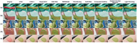
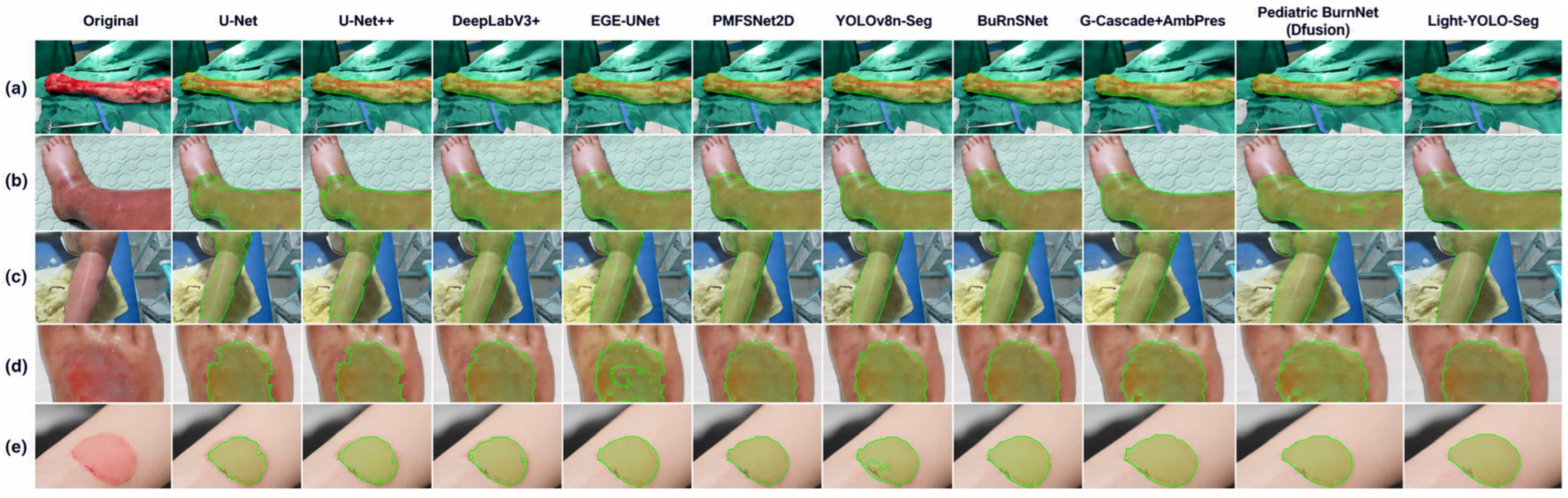
Figure 9 compares the segmentation results for 5 groups of burn wounds with different morphologies. (a)–(c) include elongated wounds, across-joint wounds, and irregular wounds, where some comparison methods exhibit local omissions or boundary shifts. The smaller wounds in (d) and (e) highlight the differences between the predicted contours and the manual annotations. In these examples, Light-YOLO-Seg covers the main wound regions more completely, maintains more continuous connections in narrow regions, and produces predicted contours that more closely follow the visible wound margins, consistent with the highest Dice and IoU results in Table 4.
Figure 9.
Segmentation results of each comparison method on 5 representative burn wounds (a–e) with different morphologies and anatomical locations.
The main differences in these complex samples are local omissions and boundary shifts. GhostV2 reduces the conventional convolution computational demands of the backbone network, and CA encodes positional information in the height and width directions within the fused neck features. Whether their combination yields consistent gains is analyzed through the ablation experiments in Section 3.5.
3.4. Comparison with Recent YOLO Instance Segmentation Models
Under the same data split and 640 × 640 input resolution, YOLOv8n-Seg, YOLOv8s-Seg, YOLOv9c-Seg [32], YOLO11n-Seg [33], YOLO26n-Seg [34], and Light-YOLO-Seg are compared (Table 5). In addition to the number of parameters and GFLOPs, Mask mAP50, Mask mAP50–95, Dice, and mBIoU are also reported to evaluate instance detection, region overlap, and boundary consistency.
Table 5.
Performance and complexity of YOLO instance segmentation models.
Light-YOLO-Seg achieves the highest values in all four metrics in Table 5: Mask mAP50, Mask mAP50–95, Dice, and mBIoU. Relative to YOLOv8n-Seg, it improves by 4.5, 5.4, 3.2, and 4.5 percentage points, respectively. The simultaneous improvement in Mask mAP50–95 and mBIoU indicates that the enhancement is reflected in both stricter instance matching and the contour overlap of matched instances.
Compared with YOLOv9c-Seg, Light-YOLO-Seg improves Mask mAP50, mAP50–95, and mBIoU by 1.2, 1.6, and 1.6 percentage points, respectively, while reducing the number of parameters and GFLOPs by approximately 89.5% and 91.3%, respectively. Compared with YOLO26n-Seg, the corresponding metrics improve by 1.5, 1.8, and 2.1 percentage points, respectively. YOLO26n-Seg has a computational cost of 9.3 GFLOPs, and YOLO11n-Seg has 2.88 M parameters. Light-YOLO-Seg achieves higher segmentation accuracy in Table 5 with 2.924 M parameters and 10.323 GFLOPs, reflecting a balance between accuracy and model size.
3.5. Ablation Experiments
3.5.1. Module Combination
Starting from YOLOv8n-Seg, configurations with only C2f-GhostV2, only three-scale CA, and both added simultaneously were trained separately (Table 6). GhostV2 replaces six internal bottlenecks in the four C2f modules of the backbone network; CA is placed after Concat and before C2f at the P3, P4, and P5 fusion nodes, with the rest of the architecture unchanged.
Table 6.
Ablation experiments of GhostV2 and Coordinate Attention.
When only GhostV2 is used, the number of parameters decreases from 3.26 M to 2.900 M, and Mask mAP50 and Mask mAP50–95 increase by 1.2 and 1.1 percentage points, respectively, indicating that the backbone replacement did not reduce segmentation accuracy in this run. When only CA is added, Mask mAP50–95 increases by 1.9 percentage points, mBIoU increases from 70.6% to 72.4%, and the number of parameters increases slightly. The combined configuration achieves Mask mAP50, Mask mAP50–95, Dice, and mBIoU of 85.3%, 61.1%, 87.2%, and 75.1%, respectively, representing increases of 4.5, 5.4, 3.2, and 4.5 percentage points over the baseline and exceeding either single-module configuration. The number of parameters remains 10.3% lower than the baseline.
When only CA is added, the three modules add 24,660 parameters. In the combined configuration, the six GhostV2 bottlenecks save 360,360 parameters; after offsetting the CA overhead, the net reduction is 335,700 parameters, resulting in approximately 2.924 M parameters, a reduction of about 10.3% relative to the baseline.
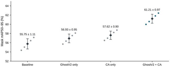
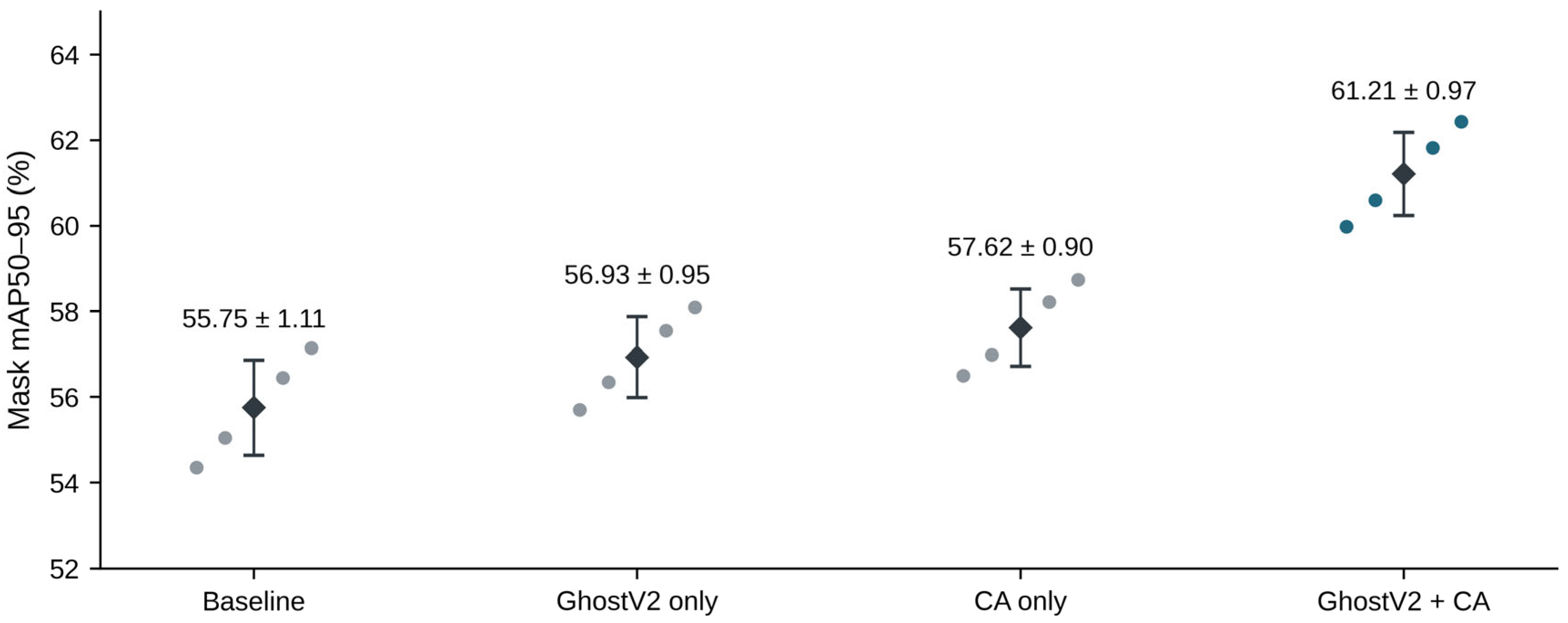
The Mask mAP50–95 of the four configurations over 5 training runs are 55.75% ± 1.11%, 56.93% ± 0.95%, 57.62% ± 0.90%, and 61.21% ± 0.97%, respectively. The combined model improves by an average of 5.46 percentage points over the baseline and is higher than the corresponding baseline under seeds 11, 22, 33, 44, and 55, with per-seed differences ranging from 5.29 to 5.63 percentage points. The combined configuration also exceeds the two single-module configurations, supporting the simultaneous use of GhostV2 and CA. Figure 10 and Appendix Table A1 present all per-run results.
Figure 10.
Mask mean average precision over IoU thresholds of 0.50–0.95 (mAP50–95) of the four module configurations across 5 seeds. Scatter points represent individual training results, and black diamonds with error bars represent the mean ± sample standard deviation. Data are shown in Table 6 and Appendix Table A1.
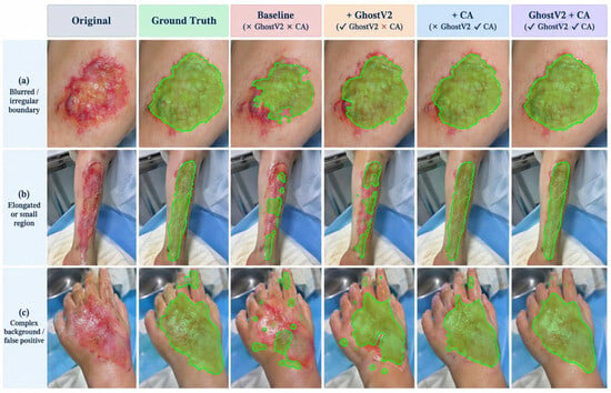
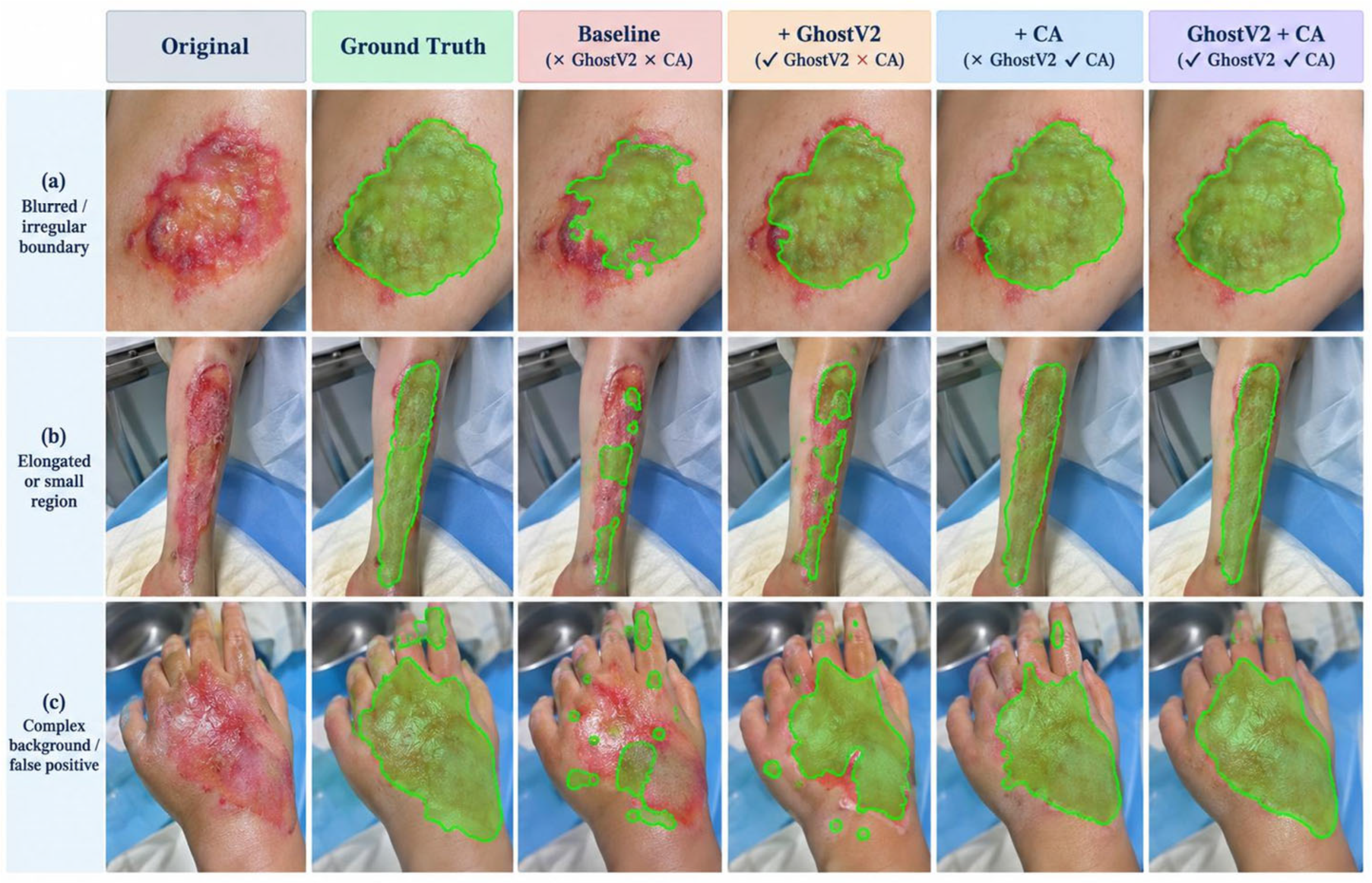
Figure 11 compares the baseline, the two single-module modifications, and the combined model. The RGB input and prediction overlay in Figure 6a are from the case shown in Figure 11a. For wounds with irregular boundaries, elongated morphologies, or strong background interference, the masks generated by the combined model are more continuous and locally more complete. These are consistent with the improvements in boundary quality and Mask mAP in Table 6.
Figure 11.
Qualitative comparison of the baseline, GhostV2 only, CA only, and the combined configuration: (a) irregular wound boundaries, (b) elongated across-joint wounds, and (c) complex backgrounds.
Under the same CA configuration, GhostV1+CA has 2.875 M parameters and a Mask mAP50–95 of 59.4%, while GhostV2+CA has 2.924 M and 61.1% (Table 7). An increase of approximately 0.049 M parameters corresponds to a 1.7 percentage point improvement in Mask AP, indicating that GhostV2 provides a better accuracy-size trade-off than this GhostV1 configuration in this task. This comparison supports the choice of GhostV2 with a DFC branch; module ablation and placement ablation separately examine its combination with CA and the CA configuration.
Table 7.
Comparison results between GhostV1 and GhostV2.
3.5.2. Coordinate Attention Placement
Keeping the four C2f-GhostV2 modules unchanged, six configurations were evaluated: no CA, P3 only, P4 only, P5 only, P3 + P4, and P3 + P4 + P5 (Table 8). P3 is the high-resolution FPN fusion node, while P4 and P5 are bottom-up PAN fusion nodes. Each CA is located after Concat and before the subsequent C2f, and the layer indices vary with the number of inserted modules.
Table 8.
Ablation experiments of Coordinate Attention placement with the GhostV2 backbone network.
Adding CA only at P3 increases Mask mAP50–95 from 56.8% to 57.5% and mBIoU from 71.1% to 72.1%, the best result among the three single-scale placements. Adding CA only at P4 or P5 yields mBIoU values of 71.9% and 71.5%, respectively. The higher spatial resolution of P3 may make it more sensitive to narrow regions and boundary positions. Combining P3 and P4 increases Mask mAP50–95 and mBIoU to 58.2% and 72.7%, respectively; adding P5 further increases them to 61.1% and 75.1%, and Mask mAP50 also rises from 82.9% to 85.3%. Although the gain from P5 alone is limited, adding P5 on top of P3 + P4 improves the three metrics by 2.4, 2.9, and 2.4 percentage points, respectively, suggesting that the broader context provided by P5 remains valuable in the combined configuration. The three-scale configuration has 2.924 million parameters and 10.323 GFLOPs.
3.6. Training Convergence
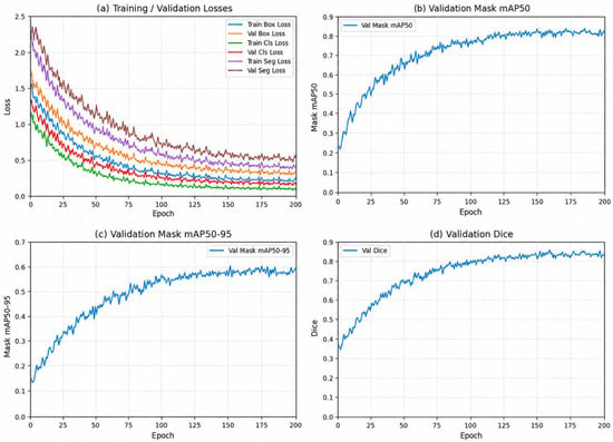
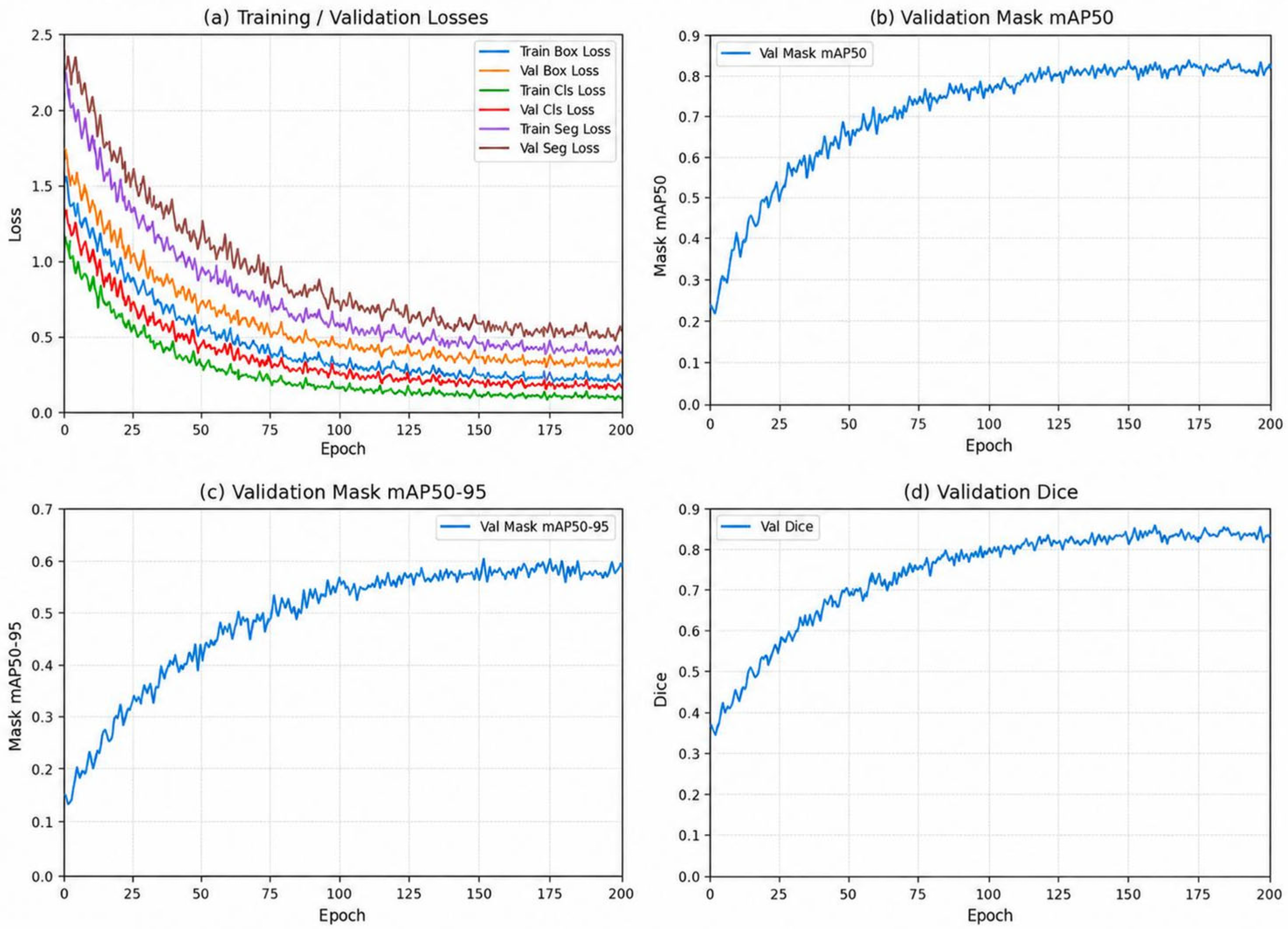
Figure 12 shows the bounding box, classification, and mask losses and the validation metrics. Losses decrease, and validation mask mAP50, mAP50–95, and Dice stabilize late in training. Table 4 and Table 5 report final performance on the 45 original test images.
Figure 12.
Training loss and validation metrics of Light-YOLO-Seg. (a) Training and validation losses; (b) validation Mask mAP50; (c) validation Mask mAP50–95; (d) validation Dice. Cls = classification and Seg = segmentation.
3.7. Edge Inference and Near-Real-Time Acquisition
Device evaluation is divided into ONNX synchronous inference on the Raspberry Pi 5 CPU and continuous operation of the collaborative system comprising the OAK-D-SR-PoE and the Raspberry Pi 5. In the CPU format comparison, each test image was inferred 50 times repeatedly, with results shown in Table 9. The collaborative system throughput is reported in Table 10. The four-model ONNX comparison in 32-bit floating-point precision (FP32) reports average latency, 95th-percentile (P95) latency, and peak process RSS in Table 11. The collaborative system response and continuous operation are reported in Table 12.
Table 9.
Synchronous inference performance of ONNX models on the Raspberry Pi 5. FP32 = 32-bit floating point and INT8 = 8-bit integer.
Table 10.
System performance in the OAK simulated wound demonstration.
Table 11.
Hardware-identical inference comparison of Raspberry Pi 5 FP32 ONNX. P95 = 95th percentile and RSS = resident set size.
Table 12.
Continuous operation and end-to-end response. P50 = 50th percentile.
The four-model test in Table 11 was uniformly executed using the ONNX Runtime 1.23.1 CPU on the Raspberry Pi 5, with the number of CPU threads set to 4. After 20 warm-up runs for each model, inference was repeated 50 times for each of the 45 test images, and the complete test was conducted independently for 3 rounds. Timing covered only model synchronous inference; image preprocessing, NMS, mask reconstruction, and display were outside the timing scope. Process RSS was sampled every 50 ms using Python psutil 7.1.1, and the peak was recorded starting from model loading. The average synchronous inference latency, P95 latency, and peak process RSS are reported.
On the tested Raspberry Pi 5 CPU backend, FP32 ONNX yields an average synchronous inference latency of 168.9 ms (5.92 FPS). With 8-bit integer (INT8) quantization, latency increases to 210.0 ms (4.76 FPS).
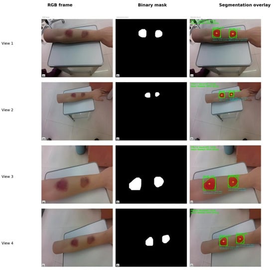
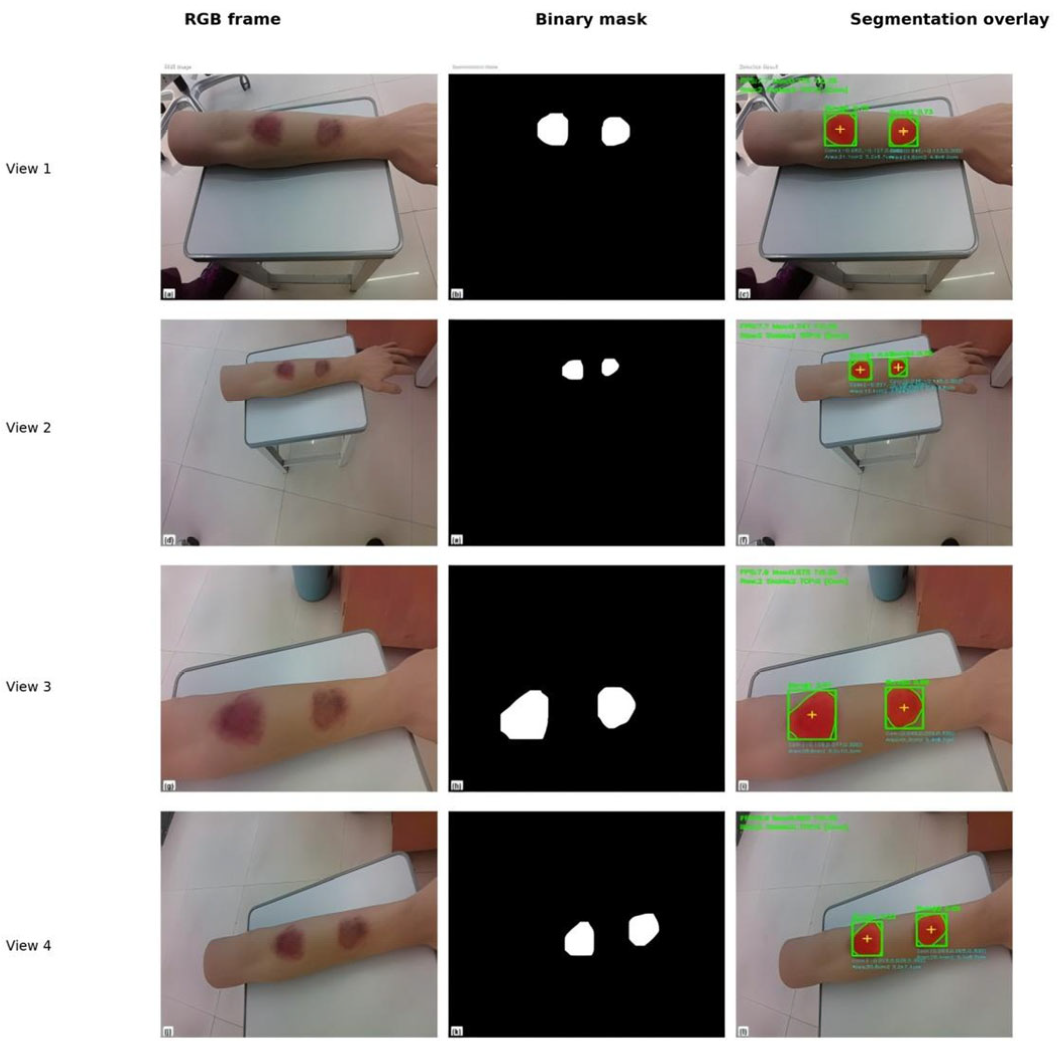
With a 640 × 640 input and a 15 FPS camera setting, the collaborative system outputs 6.9–7.9 FPS continuously (Table 10). Figure 13 shows RGB images, binary masks, and overlays at 4 viewpoints. In the representative frame, the two simulated wounds score 0.7754 and 0.7261, both above the 0.35 display threshold. These confidence scores are used solely for instance filtering.
Figure 13.
RGB frames, binary masks, and segmentation overlays of two simulated wounds on the silicone arm under 4 viewpoints in the OAK system demonstration.
The system can continuously output independent masks for the two wounds on the simulated object, demonstrating that the model conversion, VPU inference, and host post-processing pipeline can operate collaboratively. The 6.9–7.9 FPS corresponds to an average output interval of approximately 127–145 ms, supporting contour observation when the camera is mostly stable or slowly adjusted in the simulated scenarios of this study.
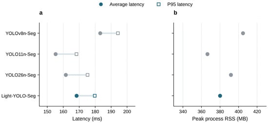
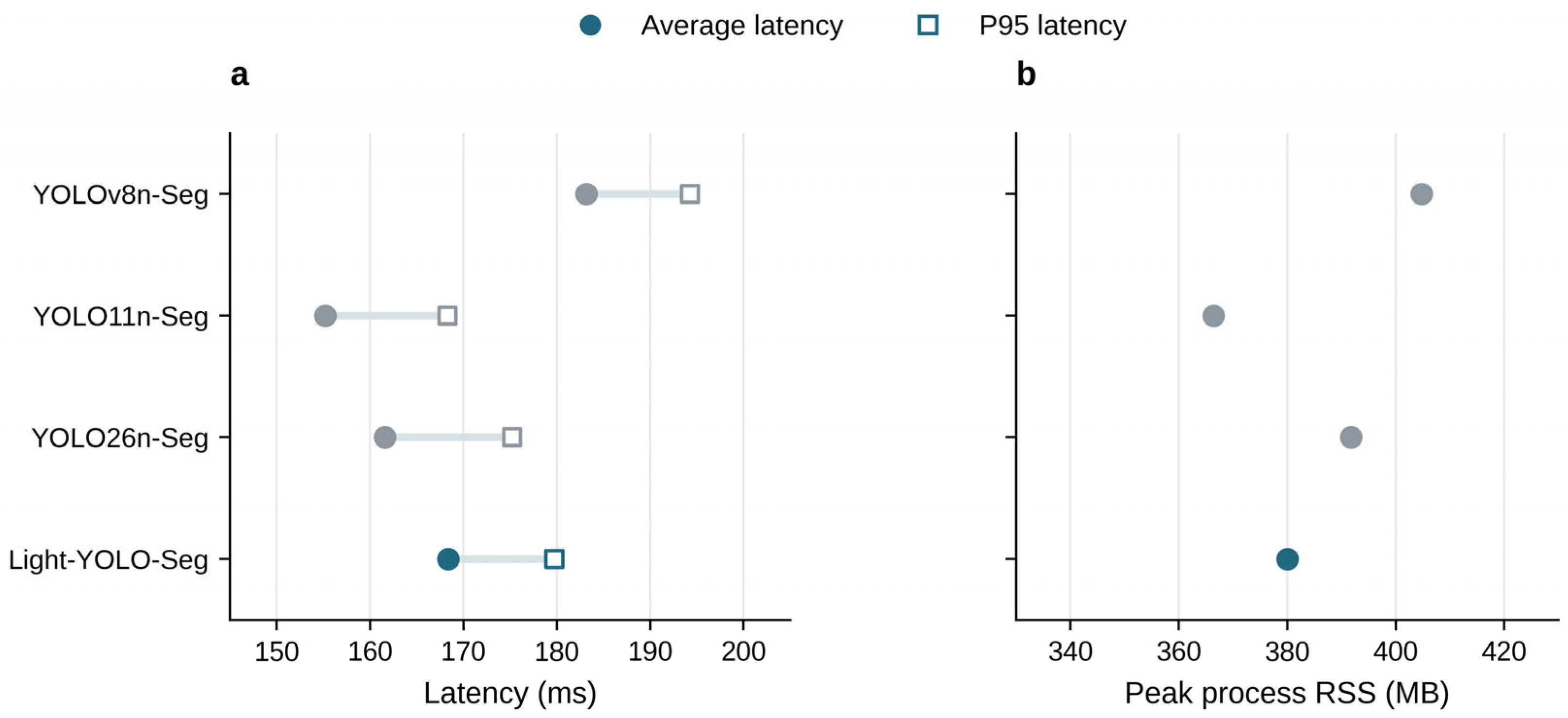
In the Raspberry Pi 5 FP32 ONNX comparison, the average latency of Light-YOLO-Seg is 168.36 ms, which is 14.79 ms (8.1%) shorter than the baseline’s 183.15 ms; the peak RSS is 380.01 MB, which is 24.80 MB (6.1%) lower than the baseline’s 404.81 MB. The device comparison in Table 11 shows that Light-YOLO-Seg has lower average synchronous inference latency and peak process RSS than YOLOv8n-Seg. The average latencies of YOLO11n-Seg and YOLO26n-Seg are 155.20 ms and 161.60 ms, respectively, which are still faster than Light-YOLO-Seg. Combined with Table 5, Light-YOLO-Seg maintains a smaller size at higher segmentation accuracy. Table 9 and Table 11 come from two sets of test records; RSS is the process resident set size.
Figure 14 compares the average latency, P95 latency, and peak RSS of the four models, presenting the numerical changes in Light-YOLO-Seg relative to the baseline and its differences from other lightweight models.
Figure 14.
FP32 ONNX inference performance on the Raspberry Pi 5. (a) Average latency and P95 latency, with lines connecting the two statistics for the same model; (b) peak process RSS, with the horizontal axis starting at 330 MB. Data are shown in Table 11.
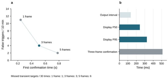
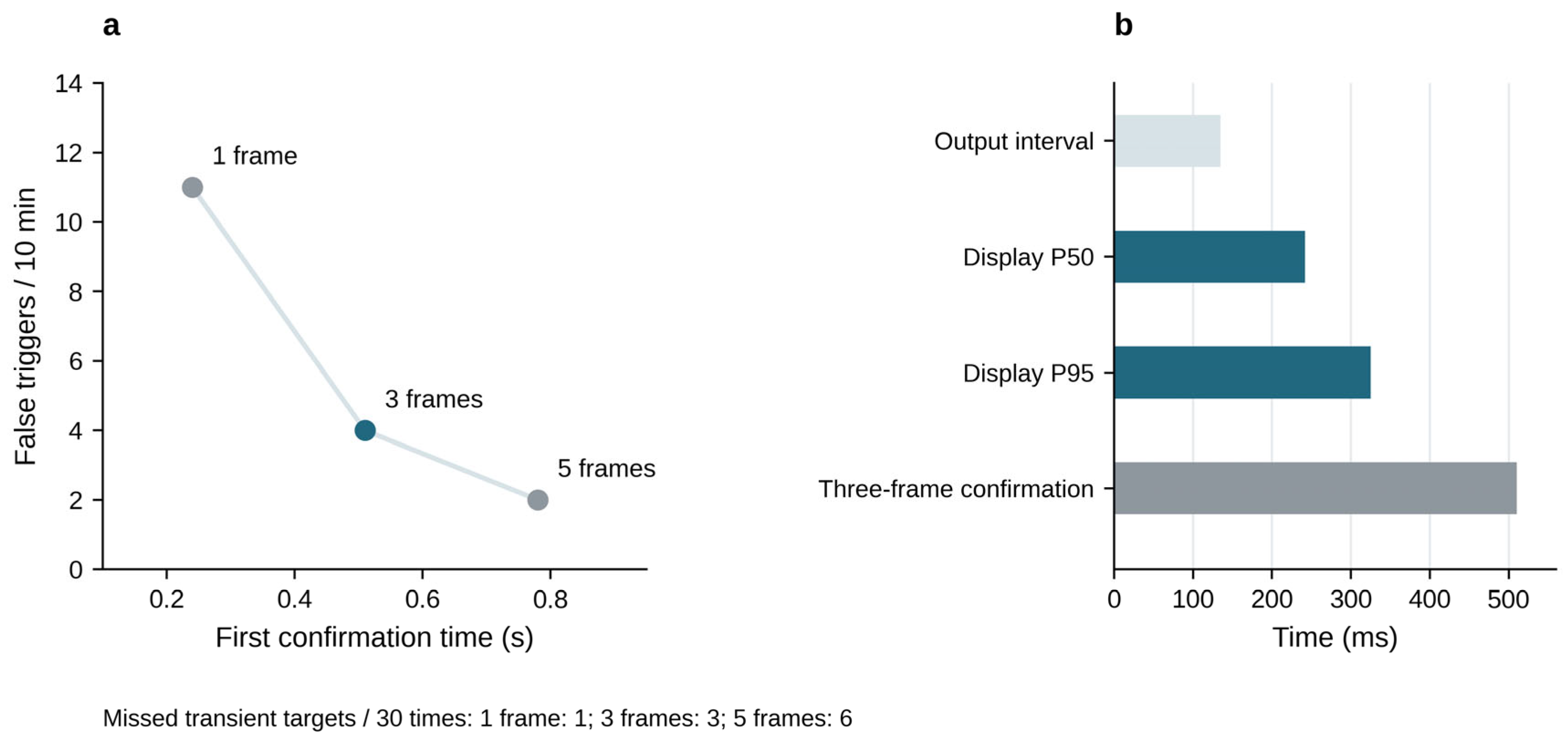
During the 120 s continuous operation, the system recorded 1788 input frames, corresponding to an actual input frame rate of 14.9 FPS. The camera was configured at 15 FPS. Counting the frames that completed inference, mask post-processing, and contour display, 888 frames were output during the same period, yielding an output throughput of 7.4 FPS, which falls within the observed range of 6.9–7.9 FPS. The average output interval is approximately 135 ms, the median (P50) and P95 latencies from frame acquisition to display are 242 and 325 ms, respectively, and the three-frame first confirmation time is 510 ms.
Compared with a single frame, three frames reduce false triggers from 11 times/10 min to 4 times/10 min, a reduction of 63.6% (Table 13); the cost is an increase in missed transient targets from 1 to 3 times/30 times and in first confirmation time from 0.24 s to 0.51 s. Five frames further reduce false triggers to 2 times/10 min but increase misses to 6 times/30 times and extend the first confirmation time to 0.78 s. Therefore, three frames were chosen to obtain the main benefit of false-trigger suppression while avoiding the higher transient target misses and the additional 270 ms confirmation delay of the five-frame scheme. The false-trigger comparison is a 10 min observation, while the throughput evaluation is a 120 s record; the two are counted separately.
Table 13.
Stability and response trade-offs of consecutive confirmation frames.
Figure 15 summarizes the stability and waiting trade-offs of the consecutive confirmation strategy and distinguishes between output interval, end-to-end latency, and first confirmation time.
Figure 15.
Consecutive confirmation strategy and system response. (a) First confirmation time and number of false triggers corresponding to the number of confirmation frames; the number of missed transient targets is labeled below the figure. (b) Output interval, P50/P95 latency from acquisition to display, and the three-frame first confirmation time. Each item corresponds to a different time metric. Data are shown in Table 12 and Table 13.
3.8. Cross-Source Evaluation and Export Precision
For cross-source evaluation, the trained Light-YOLO-Seg and YOLOv8n-Seg models were applied to 80 publicly accessible online burn wound images, with instance masks as the reference annotations (Table 14). These images did not overlap with the training images and were used only to evaluate the fixed models. The same 45 internal test images were used separately to compare mask AP before and after ONNX export.
Table 14.
Segmentation results on internal test and cross-source images.
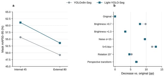
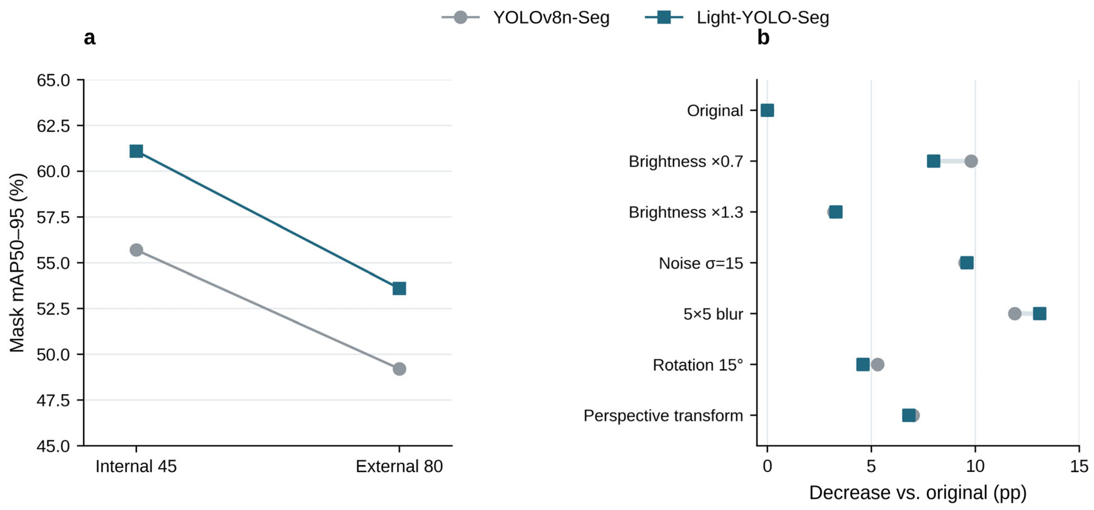
On the 80 cross-source images, the Mask mAP50–95 of Light-YOLO-Seg is 53.6%, which is 4.4 percentage points higher than the baseline’s 49.2% (Figure 16a). Dice and mBIoU are 82.7% and 68.8%, respectively, also higher than the baseline’s 79.1% and 64.6%. Compared with internal testing, the Mask AP of Light-YOLO-Seg and the baseline decreased by 7.5 and 6.5 percentage points, respectively; Light-YOLO-Seg retained a relative accuracy advantage on this batch of cross-source images. The PyTorch and ONNX Mask AP of the same 45 internal test images are 61.1% and 60.9%, respectively, indicating that the mask precision before and after export is close.
Figure 16.
Cross-source evaluation and controlled image perturbations. (a) Mask mAP50–95 of the internal 45 images and the external-source 80 images; (b) AP decrease in each model under different conditions relative to its own original image results.
3.9. Controlled Perturbations and Appearance Grouping
Brightness scaling, Gaussian noise, blur, image plane rotation, and mild perspective transformation were applied to the same 45 internal test images (Table 15) to evaluate the Mask AP under controlled two-dimensional perturbations and its decrease relative to the original image. Each derived image retained its original sample identity. Figure 13 additionally shows the qualitative output of the silicone model from four actual shooting viewpoints.
Table 15.
Mask mAP50–95 under controlled image perturbations. pp = percentage points.
The rotation condition used a fixed 15° counterclockwise rotation. In the perspective transformation, the random offset of the four image corner coordinates did not exceed 5% of the corresponding width and height, with a maximum offset of 32 pixels on 640 × 640 images. The random seed for controlled perturbations was set to 42. Geometric perturbations used the same transformation matrix for the image and the reference mask; the image used bilinear interpolation, and the mask used nearest-neighbor interpolation, preserving instance labels.
Light-YOLO-Seg is higher than the baseline under all six perturbations in Table 15, with a Mask AP advantage of 4.2–7.2 percentage points. Among them, the advantage is 7.2 percentage points at brightness ×0.7, 5.3 percentage points at σ = 15 noise, and 4.2 percentage points at 5 × 5 blur. At the same time, the AP of Light-YOLO-Seg itself decreases by 3.3–13.1 percentage points relative to the original image. The results show that the model maintains a relative accuracy advantage under the tested perturbations but is most sensitive to blur (Figure 16b). This result suggests that image sharpness is an important factor affecting deployment performance.
The practical significance of controlled perturbations lies in identifying failure tendencies. Under blur conditions, the AP of Light-YOLO-Seg drops to 48.0%, the lowest value among the listed perturbations, suggesting that sharpness degradation caused by rapid movement or defocus may weaken contour extraction performance.
The low-contrast edges, elongated or complex shapes, and multi-wound groups contain 14, 16, and 17 images, respectively (Table 16). Images may appear in more than one group. The Mask AP of Light-YOLO-Seg is 53.9%, 58.0%, and 59.0%, respectively, representing improvements of 7.1, 6.8, and 6.5 percentage points over the baseline. The absolute AP of the low-contrast group is the lowest, indicating that weak wound margins remain a difficult case; the improvement in the multi-wound group is consistent with the task objective of retaining independent instance outputs.
Table 16.
Mask mAP50–95 under appearance grouping.
4. Discussion
4.1. Segmentation Quality and Computational Demands
Compared with YOLOv8n-Seg, Light-YOLO-Seg improves the internal test Mask mAP50–95 by 5.4 percentage points and Dice by 3.2 percentage points, while reducing the number of parameters by approximately 10.3%. The five-seed average Mask AP increases by 5.46 percentage points, with the direction of gain consistent across all seeds; another controlled training run yielded a 5.5 percentage point improvement. Single comparisons, repeated training, and controlled training support the segmentation advantage of this configuration on this dataset from different experimental results.
GhostV2 reduces the conventional convolution overhead within the backbone through low-cost feature generation, while CA encodes positional information in the height and width directions within the fused features [15,16]. Both single-module configurations have higher Mask AP than the baseline, and the combined configuration further improves accuracy. Under the same CA setting, GhostV2+CA improves Mask AP by 1.7 percentage points compared with GhostV1+CA. These comparisons and the placement ablation jointly support the architectural choice of backbone compression and fusion node enhancement.
Placement ablation shows that among the single-scale CA configurations, P3 achieves the highest mBIoU. P3 uses a higher spatial resolution and preserves finer positional information. After combining P3 and P4, Mask mAP50–95 increases from 57.5% to 58.2%, and further adding P5 raises it to 61.1%. The mBIoU of the three-scale combination is 75.1%, indicating that this configuration simultaneously improves instance masks and wound margin overlap.
Comparisons with recent YOLO models reveal different trade-offs between accuracy and complexity. YOLO26n-Seg and YOLO11n-Seg have lower GFLOPs and parameter counts, respectively, while Light-YOLO-Seg achieves higher Mask AP and mBIoU. Compared with YOLOv9c-Seg, Light-YOLO-Seg improves segmentation accuracy while reducing the number of parameters and GFLOPs by approximately 89.5% and 91.3%, respectively, meeting the joint requirements of instance contour accuracy and model size in this paper.
EGE-UNet has 53,000 parameters and 0.45 GFLOPs, with Dice and wound foreground IoU that are 2.4 and 3.7 percentage points lower than Light-YOLO-Seg, respectively. This paper retains independent instance outputs for each wound; Table 4 compares foreground region coverage, and Table 5 further evaluates instance detection and boundary quality. Combined with baseline control experiments and ablation results, Light-YOLO-Seg achieves a balance between segmentation quality and model size on this dataset.
4.2. Edge Performance and Wound Documentation
In the Raspberry Pi 5 FP32 ONNX test, Light-YOLO-Seg achieves an 8.1% reduction in average latency and a 6.1% reduction in peak process RSS compared with YOLOv8n-Seg, reflecting the device-side benefits of structural compression. YOLO11n-Seg and YOLO26n-Seg infer faster, while Light-YOLO-Seg achieves higher segmentation accuracy in Table 5. A comparison of FP32 and INT8 formats shows that FP32 has lower synchronous inference latency, which aligns with the inference speed requirements on the tested CPU backend.
In the silicone simulation demonstration, the system outputs wound contours at 6.9–7.9 FPS, with an average update interval of approximately 127–145 ms (Table 10). This speed supports continuous viewing of contours at a fixed viewpoint and provides contour feedback during slow framing adjustments, serving as a reference for selecting frames for documentation. During the 120 s operation, 7.4 FPS corresponds to an update interval of approximately 135 ms, the P50/P95 latency from frame acquisition to display is 242/325 ms, and the three-frame first confirmation time is 510 ms (Table 12). These metrics collectively describe the update speed and response time of the near-real-time contour display.
The system outputs the two-dimensional contour, bounding box, and confidence for each visible wound, enabling spatially separated wounds to be viewed separately within the same frame. The contour overlay provides intuitive feedback for framing and local image documentation. Linked to existing research on burn area measurement [22], the instance contour extraction in this paper forms the basis for image region description.
4.3. Cross-Source Performance and Imaging Conditions
Cross-source evaluation supplements observations beyond the internal test set. The Mask mAP50–95 of Light-YOLO-Seg on the 80 images is 53.6%, a decrease of 7.5 percentage points compared with internal testing, but it remains 4.4 percentage points higher than the baseline on the same images. Both models exhibit performance degradation, and Light-YOLO-Seg retains a relative accuracy advantage on this cross-source set. The repeated training runs characterize variation under the fixed internal split. The cross-source comparison describes performance on the 80 online images.
Controlled perturbations and appearance grouping further illustrate the impact of imaging quality on segmentation. Under all six perturbations, the Mask AP of Light-YOLO-Seg is higher than the baseline, while its mask mAP50–95 falls by 3.3–13.1 percentage points relative to the unperturbed images. The model scores 48.0% under blur and 53.9% in the low-contrast wound margin group. Maintaining image sharpness and stable framing during system use is conducive to leveraging the continuous contour feedback.
5. Conclusions
This study constructs Light-YOLO-Seg, a burn wound instance segmentation model for edge devices. While retaining the native instance segmentation head of YOLOv8n-Seg, it replaces six conventional bottlenecks in the backbone network with GhostV2 and introduces CA at the P3, P4, and P5 fusion nodes, achieving a lightweight structural adaptation for wound contour extraction.
Light-YOLO-Seg achieves 85.3% Mask mAP50, 61.1% Mask mAP50–95, 87.2% Dice, and 75.1% mBIoU on the 45 internal test images, while reducing the number of parameters and GFLOPs by approximately 10.3% and 10.2% compared with the baseline. The five-seed average Mask AP increases by 5.46 percentage points and remains 4.4 percentage points higher than the baseline on the 80 cross-source images. In device testing, the average latency and peak process RSS are reduced by 8.1% and 6.1% compared with the baseline, respectively, and the collaborative system achieves continuous display at 6.9–7.9 FPS in the silicone simulation scenario. The study demonstrates that GhostV2 backbone compression and three-scale CA can balance burn wound instance segmentation performance and edge operational burden in this task. In the silicone phantom demonstration, the portable system supported near-real-time contour observation and image recording.
Author Contributions
Conceptualization, H.F.; methodology, R.Z., N.W., and L.L.; software, R.Z.; validation, R.Z. and L.L.; formal analysis, R.Z.; investigation, H.L.; resources, H.L. and H.F.; data curation, H.L.; writing—original draft preparation, R.Z.; writing—review and editing, H.L., N.W., L.L., and H.F.; visualization, R.Z.; supervision, N.W. and H.F.; project administration, H.F. All authors have read and agreed to the published version of the manuscript.
Funding
This research was funded by the Scientific Research Project of the Hebei Education Department (Grant No. CXZX2026003).
Data Availability Statement
Due to patient privacy and confidentiality restrictions, the burn wound image dataset analyzed in this study is not publicly available. Requests for data access should be directed to the corresponding authors. Any data sharing must comply with applicable ethical approvals, institutional requirements, and patient consent conditions.
Conflicts of Interest
The authors declare no conflicts of interest.
Appendix A. Repeated Training Results of the Four Configurations
Table A1.
Mask mAP50–95 percentages of the four configurations across 5 random seeds.
Table A1 lists the Mask mAP50–95 for 5 training runs of each of the four configurations. Calculated using the sample standard deviation, the values for the baseline, GhostV2 only, CA only, and combined configurations are 55.75% ± 1.11%, 56.93% ± 0.95%, 57.62% ± 0.90%, and 61.21% ± 0.97%, respectively.
References
- Wilson, R.H.; Rowland, R.; Kennedy, G.T.; Campbell, C.; Joe, V.C.; Chin, T.L.; Burmeister, D.M.; Christy, R.J.; Durkin, A.J. Review of machine learning for optical imaging of burn wound severity assessment. J. Biomed. Opt. 2024, 29, 020901. [Google Scholar] [CrossRef] [Scilit]
- Farhan, N.; Hassan, Z.; Ali, M.A.M.; Alqalaf, Z.; Rasul, R.E.; Jeffery, S. How Can Technology Improve Burn Wound Care: A Review of Wound Imaging Technologies and Their Application in Burns-UK Experience. Diagnostics 2025, 15, 2277. [Google Scholar] [CrossRef] [Scilit]
- Xu, X.; Bu, Q.; Xie, J.; Li, H.; Xu, F.; Li, J. On-site burn severity assessment using smartphone-captured color burn wound images. Comput. Biol. Med. 2024, 182, 109171. [Google Scholar] [CrossRef] [Scilit]
- Chauhan, J.; Rosin, P.L.; Goyal, P. BuRnSNet: Burn Region Segmentation Network from Color Images with Two-Way CNN. In Proceedings of the 2024 IEEE International Conference on Image Processing (ICIP), Abu Dhabi, United Arab Emirates, 27–30 October 2024; pp. 3172–3178. [Google Scholar] [CrossRef] [Scilit]
- Florea, L.; Florea, C.; Vertan, C.; Bădoiu, S. Ambiance Preservation Augmenting for Semantic Segmentation of Pediatric Burn Skin Lesions. Mathematics 2025, 13, 758. [Google Scholar] [CrossRef] [Scilit]
- Li, X.; Liu, Z.; Liu, L. Pediatric BurnNet: Robust multi-class segmentation and severity recognition under real-world imaging conditions. SAGE Open Med. 2025, 13, 20503121251360090. [Google Scholar] [CrossRef] [Scilit]
- Cassidy, B.; McBride, C.; Kendrick, C.; Reeves, N.D.; Pappachan, J.M.; Fernandez, C.J.; Chacko, E.; Brüngel, R.; Friedrich, C.M.; Alotaibi, M.; et al. An enhanced harmonic densely connected hybrid transformer network architecture for chronic wound segmentation utilising multi-colour space tensor merging. Comput. Biol. Med. 2025, 192, 110172. [Google Scholar] [CrossRef] [Scilit]
- Sharma, A.L.; Sharma, K.; Ghosal, P. Skin lesion segmentation: A systematic review of computational techniques, tools, and future directions. Comput. Biol. Med. 2025, 196, 110842. [Google Scholar] [CrossRef] [Scilit]
- Ronneberger, O.; Fischer, P.; Brox, T. U-Net: Convolutional Networks for Biomedical Image Segmentation. In Medical Image Computing and Computer-Assisted Intervention-MICCAI 2015; Springer: Cham, Switzerland, 2015; pp. 234–241. [Google Scholar] [CrossRef] [Scilit]
- Zhou, Z.; Siddiquee, M.M.R.; Tajbakhsh, N.; Liang, J. UNet++: Redesigning Skip Connections to Exploit Multiscale Features in Image Segmentation. IEEE Trans. Med. Imaging 2020, 39, 1856–1867. [Google Scholar] [CrossRef] [Scilit]
- Chen, L.C.; Zhu, Y.; Papandreou, G.; Schroff, F.; Adam, H. Encoder-Decoder with Atrous Separable Convolution for Semantic Image Segmentation. In Computer Vision-ECCV 2018; Springer: Cham, Switzerland, 2018; pp. 833–851. [Google Scholar] [CrossRef] [Scilit]
- Ruan, J.; Xie, M.; Gao, J.; Liu, T.; Fu, Y. EGE-UNet: An Efficient Group Enhanced UNet for Skin Lesion Segmentation. In Medical Image Computing and Computer Assisted Intervention-MICCAI 2023; Springer: Cham, Switzerland, 2023; pp. 481–490. [Google Scholar] [CrossRef] [Scilit]
- Zhong, J.; Tian, W.; Xie, Y.; Liu, Z.; Ou, J.; Tian, T.; Zhang, L. PMFSNet: Polarized multi-scale feature self-attention network for lightweight medical image segmentation. Comput. Methods Programs Biomed. 2025, 261, 108611. [Google Scholar] [CrossRef] [Scilit]
- Xu, R.; Xu, C.; Li, Z.; Zheng, T.; Yu, W.; Yang, C. Boundary guidance network for medical image segmentation. Sci. Rep. 2024, 14, 17345. [Google Scholar] [CrossRef] [Scilit]
- Tang, Y.; Han, K.; Guo, J.; Xu, C.; Xu, C.; Wang, Y. GhostNetV2: Enhance Cheap Operation with Long-Range Attention. In Advances in Neural Information Processing Systems; Neural Information Processing Systems Foundation, Inc.: San Diego, CA, USA, 2022; Volume 35, pp. 9969–9982. [Google Scholar] [CrossRef] [Scilit]
- Hou, Q.; Zhou, D.; Feng, J. Coordinate Attention for Efficient Mobile Network Design. In Proceedings of the IEEE/CVF Conference on Computer Vision and Pattern Recognition (CVPR), Nashville, TN, USA (virtual), 20–25 June 2021; pp. 13708–13717. [Google Scholar] [CrossRef] [Scilit]
- Ji, Z.; Ye, Y.; Ma, X. BDFormer: Boundary-aware dual-decoder transformer for skin lesion segmentation. Artif. Intell. Med. 2025, 162, 103079. [Google Scholar] [CrossRef] [Scilit]
- Huang, X.; Ma, Y.; Mei, X.; Wu, Z.; Sun, M.; She, Q. Lesion boundary detection for skin lesion segmentation based on boundary sensing and CNN-transformer fusion networks. Artif. Intell. Med. 2025, 167, 103190. [Google Scholar] [CrossRef] [Scilit]
- Zhu, K.; Yang, Y.; Chen, Y.; Feng, R.; Chen, D.; Fan, B.; Liu, N.; Li, Y.; Wang, X. EM-Net: Effective and morphology-aware network for skin lesion segmentation. Expert Syst. Appl. 2025, 285, 127668. [Google Scholar] [CrossRef] [Scilit]
- Yu, X.; Chen, Y.; He, G.; Zeng, Q.; Qin, Y.; Liang, M.; Luo, D.; Liao, Y.; Ren, Z.; Kang, C.; et al. Simple is what you need for efficient and accurate medical image segmentation. Expert Syst. Appl. 2026, 304, 130687. [Google Scholar] [CrossRef] [Scilit]
- Yıldız, M.; Sarpdağı, Y.; Okuyar, M.; Yildiz, M.; Çiftci, N.; Elkoca, A.; Yildirim, M.S.; Aydin, M.A.; Parlak, M.; Bingöl, B. Segmentation and classification of skin burn images with artificial intelligence: Development of a mobile application. Burns 2024, 50, 966–979. [Google Scholar] [CrossRef] [Scilit]
- Chang, C.W.; Wang, H.; Lai, F.; Christian, M.; Chen Huang, S.; Yi Tsai, H. Comparison of 3D and 2D area measurement of acute burn wounds with LiDAR technique and deep learning model. Front. Artif. Intell. 2025, 8, 1510905. [Google Scholar] [CrossRef] [Scilit]
- Zhang, Y.; Chen, Z.; Yang, X. Light-M: An efficient lightweight medical image segmentation framework for resource-constrained IoMT. Comput. Biol. Med. 2024, 170, 108088. [Google Scholar] [CrossRef] [Scilit]
- Yu, X.; Teng, L.; Zhang, D.; Zheng, J.; Chen, H. Attention correction feature and boundary constraint knowledge distillation for efficient 3D medical image segmentation. Expert Syst. Appl. 2025, 262, 125670. [Google Scholar] [CrossRef] [Scilit]
- Lee, Y.-H.; Lee, W.-B. From YOLOv1 to YOLO26: A Unified Comparative Review of the Evolution, Architecture, and Applications of YOLO-Based Object Detection Frameworks. Appl. Sci. 2026, 16, 10386. [Google Scholar] [CrossRef] [Scilit]
- Sahingoz, O.K.; Karatas Baydogmus, G.; Kugu, E. A Systematic Literature Review of You Only Look Once Architectures (v1–v12) in Healthcare Systems. Diagnostics 2026, 16, 935. [Google Scholar] [CrossRef] [Scilit]
- Baek, N.R.; Lee, Y.; Noh, D.-h.; Lee, H.-M.; Cho, S.W. AS-YOLO: Enhanced YOLO Using Ghost Bottleneck and Global Attention Mechanism for Apple Stem Segmentation. Sensors 2025, 25, 1422. [Google Scholar] [CrossRef] [Scilit]
- Luo, Y.; Zhang, K.; Wang, R.; Lei, Y. YOLOv7-PSA, an intelligent detection model, is designed for assessing the severity of skin burns. Regenesis Repair Rehabil. 2025, 1, 80–86. [Google Scholar] [CrossRef] [Scilit]
- Şevik, U.; Mutlu, O. ABC-YOLO: Automated skin burn depth classification using YOLO architectures. PLoS ONE 2026, 21, e0344042. [Google Scholar] [CrossRef] [Scilit]
- Jocher, G.; Chaurasia, A.; Qiu, J. Ultralytics YOLOv8. 2023. Available online: https://docs.ultralytics.com/models/yolov8/ (accessed on 10 October 2026).
- Cheng, B.; Girshick, R.; Dollar, P.; Berg, A.C.; Kirillov, A. Boundary IoU: Improving Object-Centric Image Segmentation Evaluation. In Proceedings of the IEEE/CVF Conference on Computer Vision and Pattern Recognition (CVPR), Nashville, TN, USA (virtual), 20–25 June 2021; pp. 15329–15337. [Google Scholar] [CrossRef] [Scilit]
- Wang, C.Y.; Yeh, I.H.; Liao, H.Y.M. YOLOv9: Learning What You Want to Learn Using Programmable Gradient Information. In Computer Vision-ECCV 2024; Springer: Cham, Switzerland, 2024; pp. 1–21. [Google Scholar] [CrossRef] [Scilit]
- Jocher, G.; Qiu, J. Ultralytics YOLO11. 2024. Available online: https://docs.ultralytics.com/models/yolo11/ (accessed on 10 October 2026).
- Jocher, G.; Qiu, J.; Liu, M.; Lyu, S.; Akyon, F.C.; Kalfaoglu, M.E. Ultralytics YOLO26: Unified Real-Time End-to-End Vision Models. arXiv 2026, arXiv:2606.03748. [Google Scholar] [CrossRef] [Scilit]

Disclaimer/Publisher’s Note: The statements, opinions and data contained in all publications are solely those of the individual author(s) and contributor(s) and not of MDPI and/or the editor(s). MDPI and/or the editor(s) disclaim responsibility for any injury to people or property resulting from any ideas, methods, instructions or products referred to in the content. |
© 2026 by the authors. Licensee MDPI, Basel, Switzerland. This article is an open access article distributed under the terms and conditions of the Creative Commons Attribution (CC BY) license.