


Abstract
Predicting flood dynamics in data-scarce urban catchments remains a major hydrological challenge, yet physically-based modeling is essential for design mitigation infrastructure. This study assessed the impact of land cover change on the hydrological response and hydraulic performance of the ungauged Kinalumsan River in Cebu City, Philippines, which frequently overflows during intense rainfall. To overcome the absence of historical gauge records, a short-term field monitoring campaign was conducted to capture discrete storm events for event-based calibration. Land cover maps from 1996 to 2023 were analyzed to evaluate spatiotemporal trends. A physically-based, coupled modeling framework was deployed: a HEC-HMS model utilized the Soil Conservation Service Curve Number (SCS-CN) method to simulate peak discharges under 10-, 25-, 50- and 100-year return periods, which subsequently drove a HEC-RAS (Version 6.6) 2D model to assess flood characteristics. The event-based calibration demonstrated good predictive performance, achieving Nash–Sutcliffe Efficiency (NSE) values of 0.96 (HEC-HMS) and 0.88 (HEC-RAS), indicating reliable simulation of the catchment’s response. Results show a steady increase in built-up areas, which contributed to higher peak discharges and expanded flood extents. Extreme rainfall events further amplified flood hazards, with the 100-year return period producing the widest inundation. The districts of Tisa and Punta Princesa located near the downstream portion of the Kinalumsan River consistently experienced the greatest exposure in both depth and velocity terms. Overall, the study demonstrates that integrating short-duration monitoring campaigns with coupled hydrologic–hydraulic modeling provides a scientifically defensible, highly transferable template for rapid flood hazard mapping and stormwater management in data-constrained developing regions. This cost-effective method of flood modelling can be upscaled to other cities where data is scarce including selection of nature-based solutions for the improvement of urban drainage and stormwater management for resilient cities.
1. Introduction
Flooding represents one of the most destructive natural hazards globally, threatening human safety, critical infrastructure, and socio-economic stability [1]. In Asia, over 80% of reported hydrometeorological disasters are driven by severe storm and flood events [2]. These challenges are particularly intense in the Philippines, which experiences an average of 20 tropical cyclones annually, subjecting rapidly expanding urban centers like Metro Cebu to frequent and severe inundation [3,4]. Urban flood risk is further amplified by rapid land use shifts; globally, over 55% of the population resides in urban areas—a figure projected to rise significantly by 2050 [5]. In highly urbanized coastal centers such as Cebu City, where urbanization has reached 94% [6], the conversion of permeable natural landscapes into impervious surfaces reduces infiltration capacity, accelerates peak runoff generation, and shortens catchment response times [7,8]. When combined with undersized, debris-clogged drainage channels, high-intensity storm events frequently exceed channel conveyance capacities, leading to severe localized flash flooding [9].
Assessing land use change impacts and predicting peak hydrographs in ungauged or data-scarce urban catchments remains a major hurdle in modern hydrology [10,11]. To evaluate flood exposure and land use dynamics, the recent literature has increasingly relied on a top-down approach using data-driven, geospatial, and remote sensing techniques. For instance, advanced spectral indices combined with machine learning algorithms like Random Forest classifiers have proven effective for rapid, broad-scale surface water detection and flood susceptibility mapping [12]. Similarly, spatial geostatistical indices have been widely deployed to quantify spatial dependencies between landscape patterns, land cover transitions, and environmental risk [13].
While remote sensing indices, machine learning algorithms and geostatistical approaches offer valuable visualization of inundation footprints and land use risks without requiring complex boundary condition hydrographs, they are fundamentally empirical. They generally lack physical conservation of mass and momentum, limiting their ability to simulate explicit hydrograph timing (), peak discharge attenuation (), or dynamic 1D/2D hydraulic surface profiles under specific storm design scenarios [11]. These metrics are essential for sizing structural flood mitigations and drainage infrastructure. To capture these physical dynamics, physically-based hydrological and hydraulic modeling like the coupled Hydrologic Engineering Center’s Hydrologic Modeling System (HEC-HMS) and River Analysis System (HEC-RAS) frameworks remains the benchmark standard [14]. Although deploying such models in ungauged tropical catchments where long-term hydrometric monitoring is absent introduces some parameter uncertainty, event-based calibration and validation using discrete observed rainfall–runoff events represents an established, scientifically defensible modeling approach [15,16]. Coupled HEC-HMS and HEC-RAS frameworks have been successfully calibrated on discrete storm events to isolate the specific impacts of land use and land cover (LULC) transitions on Curve Numbers (CNs), peak runoff hydrographs (Qp), and downstream hydraulic profile elevations [17,18]. These studies show that short-duration monitoring campaigns capturing typical discrete storm events can sufficiently parameterize physically-based models, establishing a validated baseline hydrological framework for rapid flood hazard mapping in data-constrained environments.
To address these methodological and data availability constraints, this study evaluates a rapid, short-term monitoring workflow integrated with a coupled hydrologic–hydraulic modeling framework. Focusing on the urbanized, ungauged Kinalumsan River basin in Cebu City, Philippine which experienced severe overflowing during intense rainfall events, this research utilizes a short-term (2–3 month) field monitoring campaign to capture discrete storm events for model calibration and validation. By evaluating the performance of event-based HEC-HMS and HEC-RAS models driven by local land cover transitions, this study provides a transferable template for rapid flood hazard mapping and drainage assessment in data-poor urban catchments across developing regions.
2. Study Area
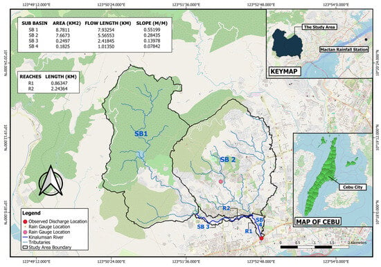
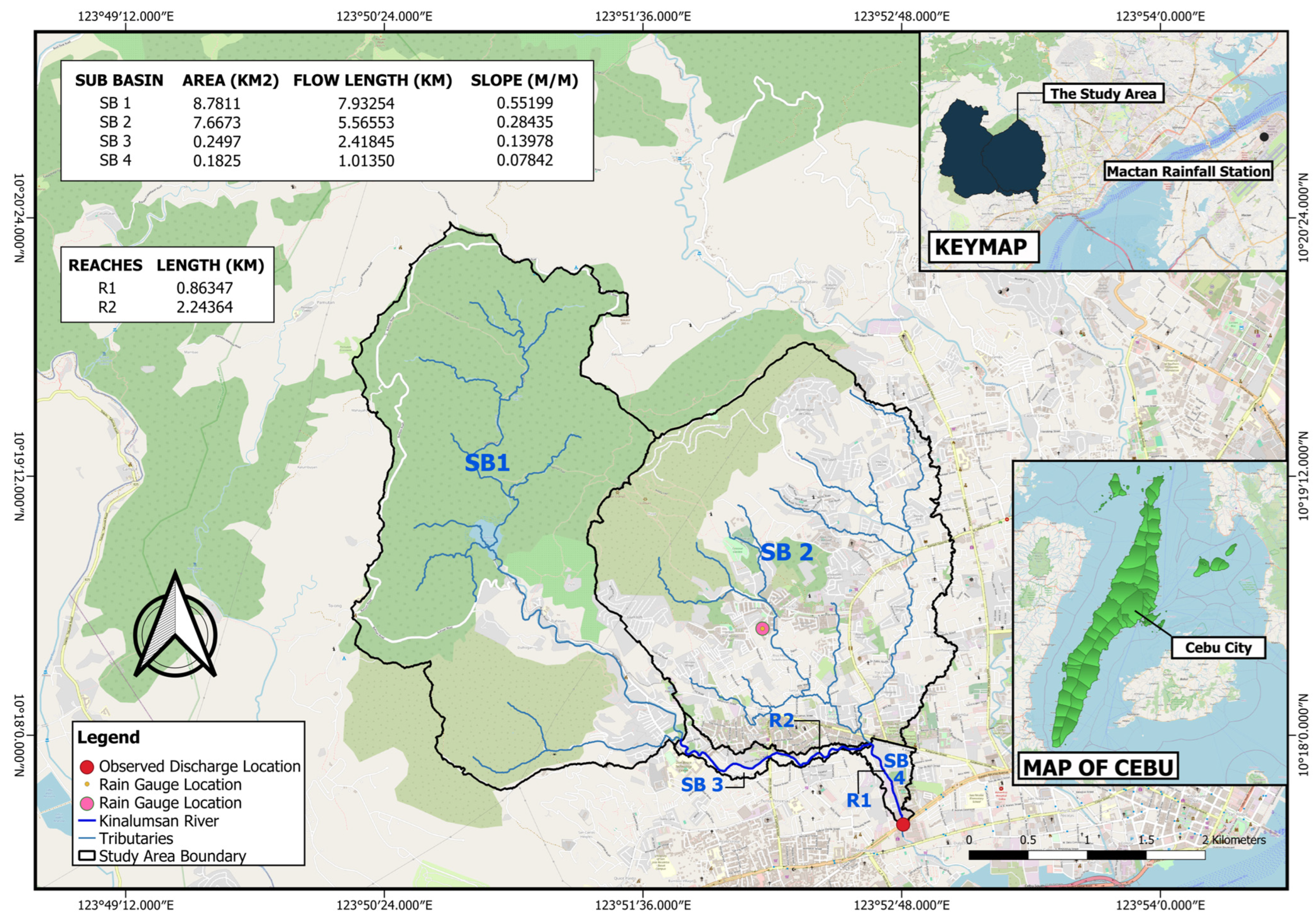
The Kinalumsan River is one of the major rivers in Cebu City situated in Cebu, Central Visayas, Philippines, that traverses the uptown barangays of Buhisan and Labangon, and downtown barangays of Tisa, Mambaling and Duljo Fatima (Figure 1). Barangay is a term locally used to denote small villages or districts making up a city. The chosen outlet point of the study lies in the downstream portion of the river specifically at Kinalumsan Bridge 1 along N. Bacalso Avenue, Brgy. Mambaling, Cebu City with coordinates 10°17′35.4″ latitude and 123°52′48.7″ longitude. The delineated catchment of Kinalumsan River with its outlet (shown in Figure 1) has a total area of 16.88 km2 that is located within the jurisdiction of Cebu City, encompassing the political boundaries of Barangays Labangon, Tisa, Buhisan, Guadalupe, Mambaling, Pamutan, Punta Princesa and Pardo.
Figure 1.
Delineated Catchment of Kinalumsan River.
3. Material and Methods
3.1. Objectives of the Research Work
The specific objectives of the research work are to determine the rate of change of land cover within the catchment of Kinalumsan River between 1996 to 2023, to project discharge of the catchment due to land cover alteration and assess the performance of Kinalumsan River in terms of capacity, average velocity, and hydraulic grade line (water level) from 1996 to 2023, and to evaluate the impact of different extreme rainfall events on flood depths, flood extent, and water velocity from 1996 to 2023.
3.2. Data Collection and Pre-Processing
Table 1 summarizes the data used in the study including their description, corresponding sources, and data type.
Table 1.
Summary of data types and sources relevant in the study.
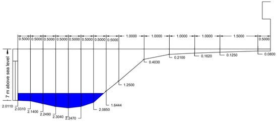
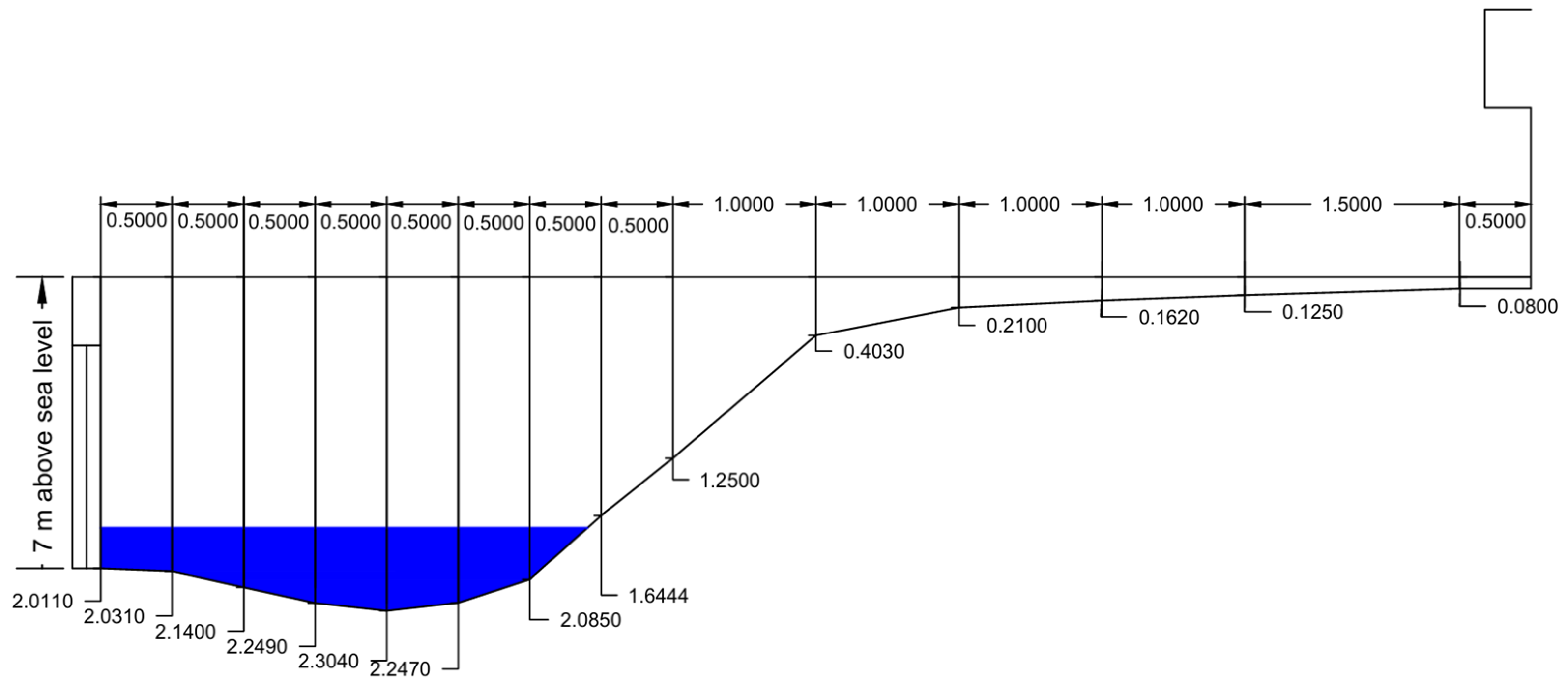
The Kinalumsan River catchment boundary was delineated from a 1 m × 1 m DEM acquired from LiPAD website using HEC-HMS and QGIS. The land cover maps of the study were developed using Landsat 5, 8, and 9 images with a 30 m spatial resolution obtained from Earth Explorer website. Rainfall data and stream flow data were collected between March and May 2025. For the rainfall data, a tipping bucket rain gauge was installed approximately in the center of the catchment area, with specific coordinates of 10°18′36″ N and 123°52′12″ E. The Rainfall Intensity Duration Frequency (RIDF) curves used in this study were based on the 35 years of record prepared by the state-run weather agency, PAG-ASA, for the Mactan station. At least 30 streamflow measurements were conducted at the outlet point of the study area (Kinalumsan Bridge 1) and from it, a stage–discharge relationship was established, from which discharge values were predicted and utilized as inputs for hydrological modeling in HEC-HMS. Water levels were recorded continuously using a video recording camera faced at a staff gauge installed along the river embankment, yielding at least 30 stage readings. River velocity was measured using the float method with an orange fruit as a floating device. Measurements were taken from the left, middle, and right sections of the river as viewed facing downstream. In order to obtain the mean velocity of the water, a correction factor of 0.85 was applied to the measured water surface velocity [19,20]. The river’s cross-section was surveyed by measuring an approximate 10 m width and collecting depth data at eight sections, as seen in Figure 2.
Figure 2.
River’s cross-section profile (m).
3.3. Rate of Change in Land Cover
The initial step in processing the Landsat images was collecting the important images of the satellite between 1996 and 2023. Images from Landsat 5, 8, and 9 were used because of their high spatial resolution. The Semi-Automatic Classification Plugin (SCP) in QGIS was used for the classification of land cover. Four major land cover classes were identified in the study area: (1) built-up area, (2) bare area, (3) open forest, and (4) shrubland. These classes were chosen based on their dominance within the catchment area, with the numbers representing their class IDs. The classified land cover maps for years 1996, 2005, 2014, and 2023 were compared to determine the land cover changes and QGIS was then used to perform a change detection analysis on these maps. The areas for each land cover type for the different years were determined and the rate of change for the periods 1996–2005, 2005–2014, and 2014–2023 were calculated to analyze land cover change in the study area. In generating CN grids, the obtained soil data from the Geoportal PH was merged with the land cover data. Based on the soil type map acquired from the Geoportal PH, the catchment contained clay and clay loam. With this, the researchers used the Hydrologic Soil Group D (clay loam, sandy clay, silty clay loam, silty clay, clay) as the soil type of the study’s catchment area.
3.4. Hydrologic Analysis Using HEC-HMS
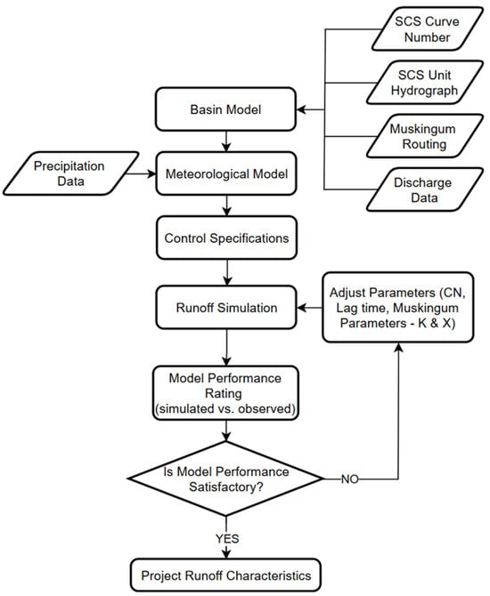
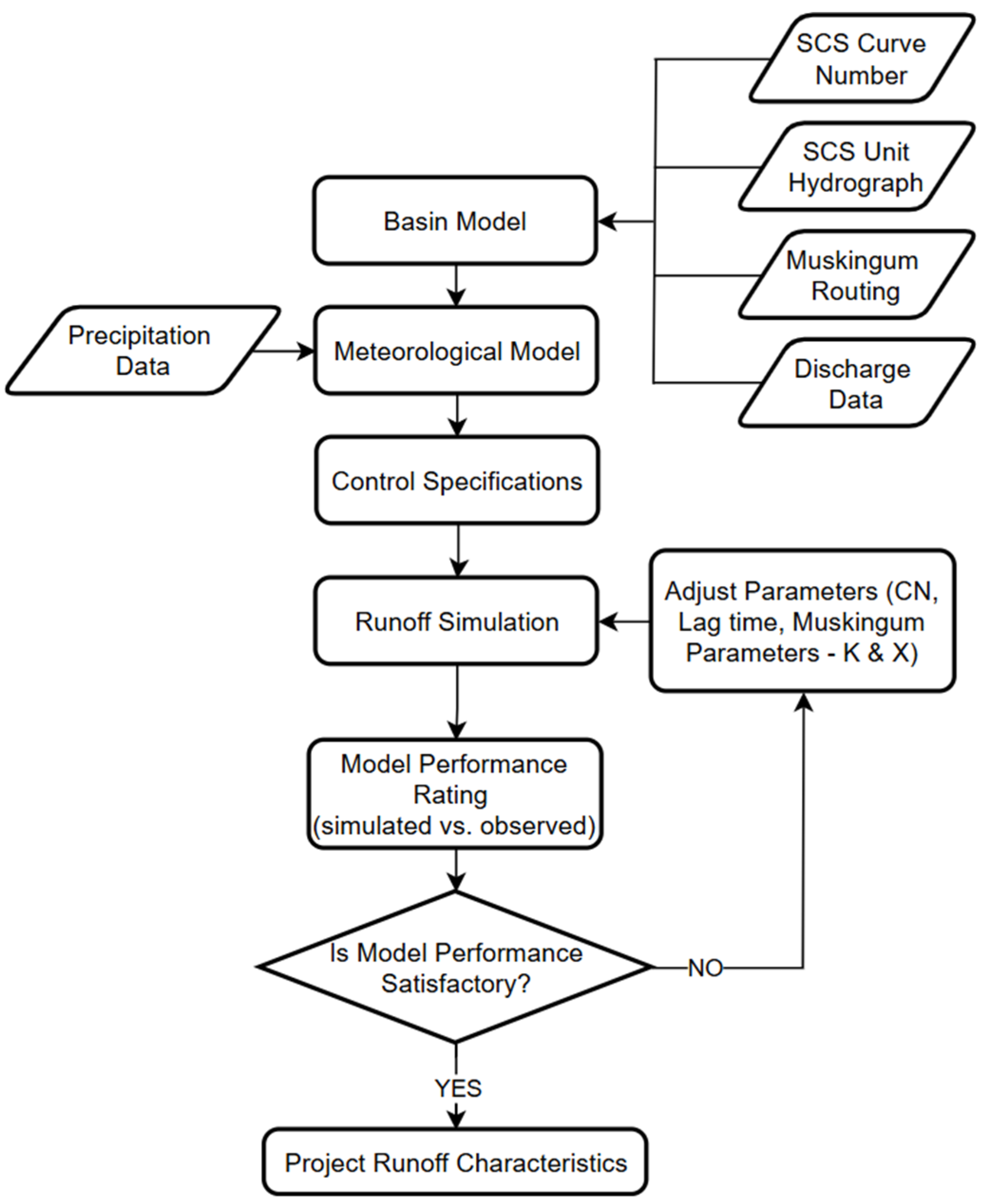
A flowchart of how the HEC-HMS model was developed is shown in Figure 3. Several input parameters acquired from various secondary sources (Table 1) like rainfall and actual streamflow data gathered during the short monitoring period were used.
Figure 3.
HEC-HMS flowchart.
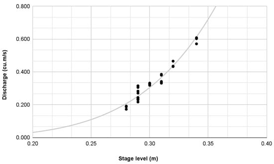
A rainfall–runoff model was generated for the Kinalumsan River basin. Using the 10-, 25-, 50-, and 100-year storm return periods, the hydrologic response of the catchment was simulated using the hydrologic model developed. The SCS-CN model was chosen as the loss model because of its simplicity. It estimates the excess of precipitation based on soil cover, antecedent moisture, cumulative precipitation, and land use [21]. The transform model utilized was the SCS Unit Hydrograph which only requires the calculation of lag time. The lag time was taken to be equal to 0.6 Tc and the time of concentration was estimated using the watershed lag method equation. Muskingum method was selected as the channel flow routing method because it is highly suitable for event-based simulations, requires fewer parameters, and detailed channel geometry for the entire river is not available. The Muskingum parameters K = 0.5 and X = 0.25 were assumed and initially assigned to all reaches and these initial values were then modified during the calibration process. All the parameters used for the hydrologic model are in Appendix A. For the meteorological model, a Specified Hyetograph was used as a precipitation method. The Alternating Block Method was used in creating the rainfall temporal distribution by designing a hyetograph using the Philippine Atmospheric, Geophysical and Astronomical Services Administration (PAGASA) Mactan Rainfall Intensity Duration Frequency (RIDF) curve [22]. During calibration, the model’s parameters such as the curve numbers, initial abstraction, and the Muskingum (X & K) parameters were adjusted in order to achieve a better fit and adequately match the simulated with the observed data. The discharge data at the watershed’s outlet was obtained indirectly by establishing a stage–discharge relationship for the stream [23]. The resulting rating curve equation (Equation (1)) was used to transform the observed stages into the corresponding discharges. The Nash–Sutcliffe Efficiency (NSE), Ratio of the Root Mean Square Error to the Standard Deviation Ratio (RSR), and Percent Bias (PBIAS) were determined to be able to assess the hydrological model performance. These calibration statistics were based on the interpretations of Moriasi et al. [24] and were utilized to be able to compare the simulated and observed hydrographs.
Q = 27.6849 (S − 0.2)1.9521
Caution must be exercised in the interpretation of the historical flood reconstructions as they do not necessarily reflect the actual catchment response for the periods considered. They serve only as a baseline scenario to better understand the dynamics of a changing landscape to the generated flood peaks and flooding volume.
3.5. 2D Flood Simulation Using HEC-RAS
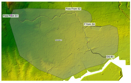
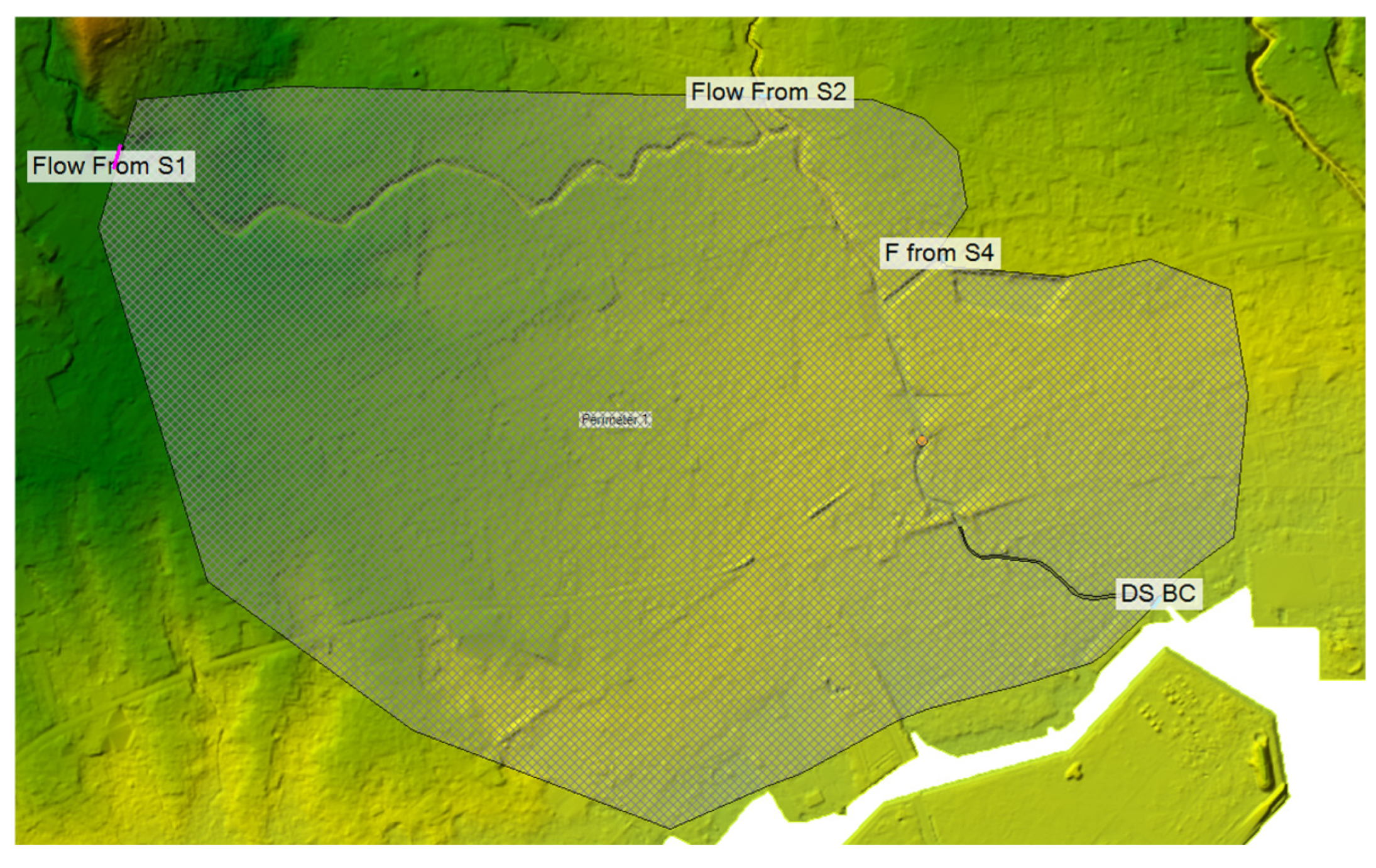
HEC-RAS is a software package that performs two-dimensional (2D) hydraulic modeling and is ideal for simulating water movement through river channels and other flow areas. While the one-dimensional approach is suitable for regular channels, the 2D approach is used primarily for complex channels and terrain such as Kinalumsan River and the area around it [25]. Figure 4 shows the boundaries of the 2D model.
Figure 4.
HEC-RAS 2D model extent.
3.5.1. Governing Equations in HEC-RAS Modeling
In HEC-RAS, the hydrodynamic calculations were based on the Saint–Venant equations. These equations determined open-channel flow and also included the continuity equation, which had mass conservation and momentum equation. These take into account forces like gravity, friction, and pressure gradients. 2D modeling used shallow water equations that were simplified, and flow in x directions and y directions. The continuity equation is
where A is the cross-sectional flow area, Q is the discharge, x is the longitudinal distance, and t is time. The Momentum Equation is
where g is the acceleration due to gravity, h is the water depth, if the friction slope, and is the bed slope.
2D Shallow Water Equations. In floodplain modeling, the shallow water equation used is
where h is the water depth, and are the specific discharges in the x and y direction, respectively. These equations guarantee that the model captures overland flow movement, because it is vital in the simulation of flood behavior under different land cover scenarios [25].
3.5.2. Land Cover Changes and Parameter Integration
This section described how land cover changes were incorporated into the hydrological and hydraulic parameters. This was important, as flood scenarios simulated in HEC-HMS and HEC-RAS were based on land cover. The theoretical procedure for scenario-based studies was provided by the explanation of Manning’s roughness coefficient n, infiltration rates, and impervious surfaces. It was important that land cover changes were integrated properly in the model, as it would make it accurate. Key parameters affected by land cover are as follows:
Manning’s Roughness Coefficient (n). Different land cover types had influence on flow resistance. Usually, urbanized areas had lower n, while vegetated areas produce higher n values [26]. For instance, Vashist and Singh [26] emphasized that assigning accurate n values for different types of land cover, while taking into account different land cover types, was important for accurate flood modeling. Manning’s equation is vital for understanding this relationship:
where V is the flow velocity, n is Manning’s roughness coefficient, R is the hydraulic radius, and S is the slope of the energy grade line.
Infiltration Rates. Urbanization reduced infiltration due to impervious surfaces, which increased runoff. Hydrologic soil group classifications and impervious surface ratios should align for each scenario. A common observation made to areas with great changes in land cover due to urbanization experienced different responses to rain, like higher runoff peaks and shorter lag times [26]. In modeling, infiltration rates can be described through Horton’s infiltration equation:
where is the infiltration rate at time t, is the initial infiltration rate, is the final infiltration rate, and k is the decay constant.
3.5.3. Calibration of HEC-RAS Model
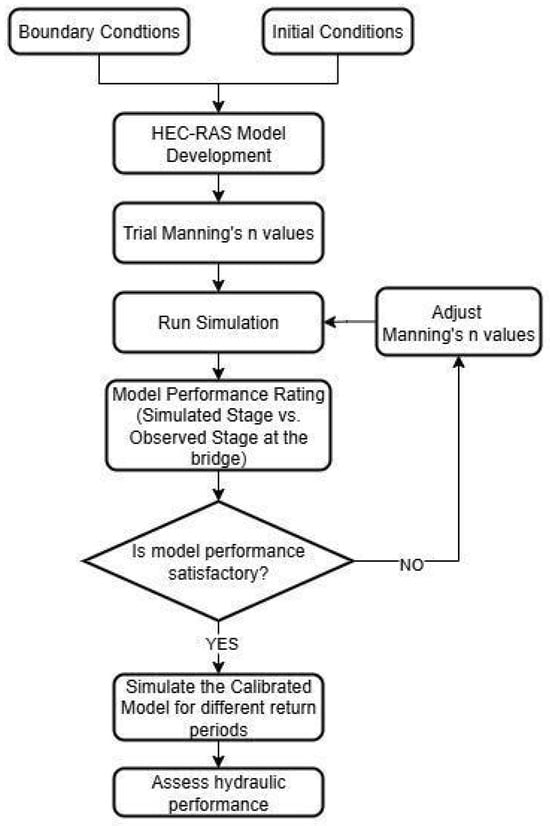
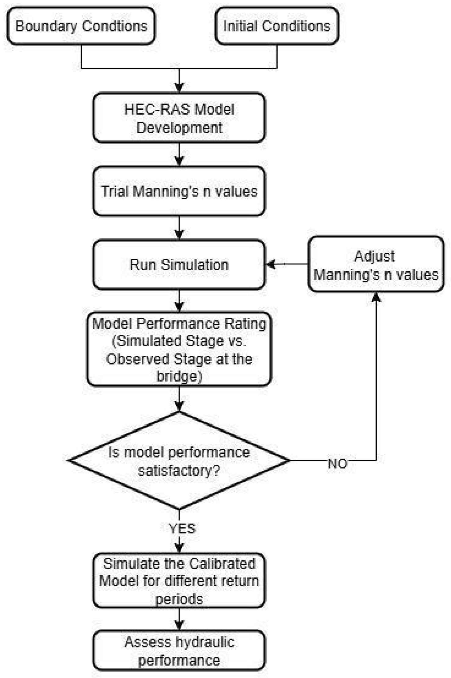
The flowchart on the HEC-RAS calibration procedure is shown in Figure 5. Building a HEC-RAS model starts with the determination of boundary and initial conditions. The Manning’s roughness parameters were estimated based on the land cover map generated for the year 2023. For the downstream boundary condition, the normal depth was used, which required an input of 0.003 friction slope for the reach and uses Manning’s equation to estimate a stage for each computed flow. For the unsteady flow analysis set-up, a computation interval of 1 min was used, along with an output interval of 5 min, a mesh size of 5 × 5 and a simulation period that lasted 6 h. In calibrating the 2D model in HEC-RAS, the model’s roughness coefficients (Manning’s n) of the channel were adjusted for both the main channel and the floodplain to make the simulated stage closely match the observed stage recorded at the outlet. The Nash–Sutcliffe NSE, and RMSE were determined to be able to assess the hydraulic model performance.
Figure 5.
HEC-RAS flowchart.
3.5.4. Model Validation for HEC-RAS 2D Simulations
Model validation was vital in ensuring a level of confidence of the integrated 2D flood simulations in HEC-RAS before moving on to the scenario analysis. Validation involves the following:
- Flood Survey. Flood data at multiple locations along the Kinalumsan River were collected either by field surveys or data collection. Interviews with residents around the area provided additional information on the details of flooding during rainfall.
- Flow Velocity Measurements. Instantaneous flow velocity measurements were attained from known data.
- Sensitivity Analysis. Manning’s coefficients were adjusted to see how it affects velocity, using Equation (4). However, since the study’s main focus lies on estimating the impact of land use and land cover change to the watershed’s response, the development of a flood hazard map with high accuracy is not a main goal.
The validation of the model’s simulated results was compared with actual measurements. The following steps were done in order to achieve this:
- Selection of Validation Data. Stage data was collected at the outlet using a low-cost instrumentation—a camera coupled with a staff gauge. The calibrated model’s simulated stage was then compared with a separate rainfall event’s stage. Validation metrics were used to define how satisfactory the calibrated then validated model was.
- Calibration Parameters. For the 2D model, Manning’s roughness coefficients of the floodplain and contraction and expansion coefficients were adjusted in order to improve accuracy of the model.
- Validation Metrics. The performance of the model was evaluated with the Nash–Sutcliffe Efficiency (NSE). This validation metric was based on the interpretations of Moriasi et al. [24] and was utilized to be able to compare the simulated and observed hydrographs.
- Validation Results. The NSE generated determined the performance of the model [24]:
NSE > 0.75: Very good agreement
0.5 ≤ NSE ≤ 0.75: Satisfactory
NSE < 0.5: Unsatisfactory
If the validation results achieved were unsatisfactory, the model parameters were refined and adjusted until the desired satisfaction was achieved. This process validated the accuracy of the 2D HEC-RAS model.
- Rainfall Scenario Definitions. Rainfall scenarios were defined to evaluate the impact of different rainfall intensities and durations on flooding. These scenarios were based on Rainfall Intensity–Duration–Frequency (RIDF) curves from PAGASA. Four return periods (10-, 25-, 50-, and 100-year events) were used to represent low, medium, high and extreme rainfall events, respectively. The rainfall data was assumed to be uniform across the catchment. This simplifies the analysis and still captures the response hydrologically to extreme rainfall events [27]. In order to simulate the rainfall–runoff process for the different scenarios, RIDF curves were used to estimate the intensity of rainfalls based on duration and probabilities of storms. These intensities were then integrated into HEC-RAS, which were used to represent the hydrological response of the area. Through standardized RIDF curves, the analysis on the impacts of different rainfall intensities on flooding were consistent.
3.5.5. Flood Hazard Map Generation and Comparative Analysis
The simulation results from HEC-RAS were integrated into GIS, creating flood maps visualizing flood depth, extent, and velocity. Flood depth maps showed the vertical depth of floodwaters, with severity levels categorized into minor, moderate and severe. Flood extent maps showed the horizontal spread, or the extent, of flood. Water velocity maps showed different areas with different flood water velocity, where higher velocity tended to indicate hazardous zones [28].
Lastly, a comparative analysis was done to investigate how the outputs above changed across the different urbanization and rainfall scenarios. Outputs from 1996–2023 land cover change scenarios were compared under the four rainfall return periods (10, 25, 50, and 100). The results were shown and analyzed through the maps and charts, highlighting areas with significant changes in flood characters and areas at higher risk of flooding.
4. Results
4.1. Land Cover Analysis
Land Cover Classification and Accuracy Assessment
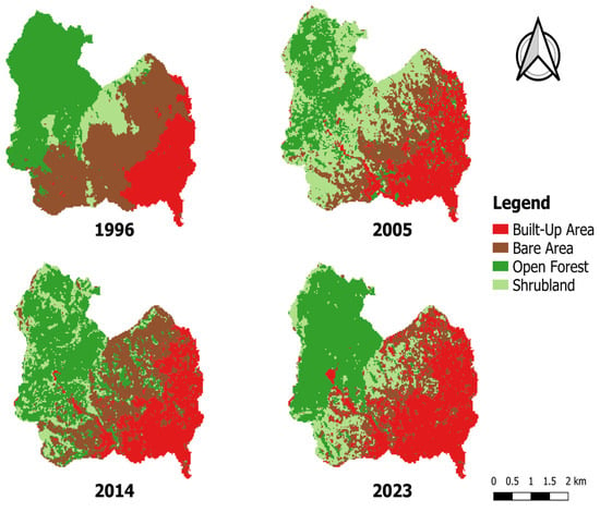
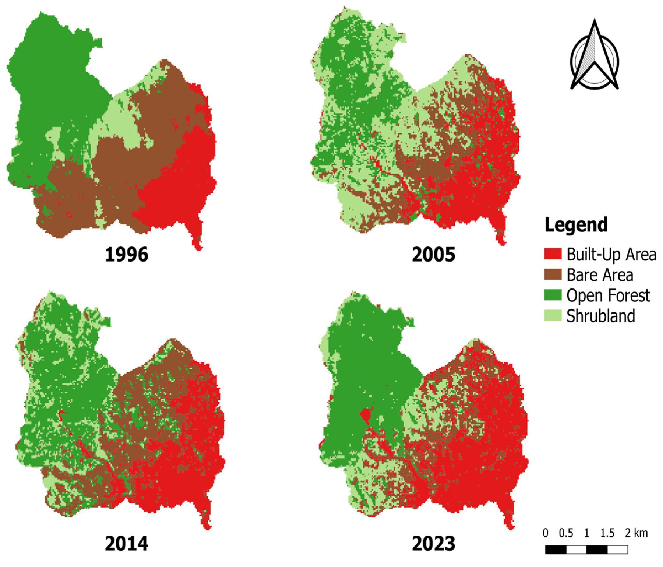
Figure 6 illustrates the land cover classification maps for years 1996, 2005, 2014, and 2023. Figure 3 illustrates the land cover classification maps for years 1996, 2005, 2014, and 2023. The reliability of the classified land cover maps was confirmed through confusion matrix analysis using the QGIS Semi-Automatic Classification Plugin (SCP). The classification achieved an overall accuracy of 87.466% (1996), 95.254% (2005), 93.984% (2014), and 96.317% (2023), and corresponding kappa hat values of 0.8127, 0.9309, 0.9021, and 0.9391, indicating strong agreement with reference ground truth data. Producers’ accuracies ranged from 37.4458% to 100% in 1996, 81.864% to 98.7338% in 2005, 78.874% to 100%, and 80.9075% to 97.6597% in 2023, while users’ accuracies ranged from 70.9302% to 98.8571% in 1996, 83.7209% to 100% in 2005, 32.1429% to 100%, and 62.500% to 98.6301% in 2023 across all land cover classes. Omission and commission errors were minimal, primarily occurring along transition zones between shrubland and bareland. The class-specific accuracy metrics are summarized in Table 2, and the rest are found in Appendix B Table A6, Table A7, Table A8 and Table A9.
Figure 6.
Land cover classification maps for 1996, 2005, 2014, and 2023.
Table 2.
2023 Land cover accuracy assessment.
4.2. Land Cover Change
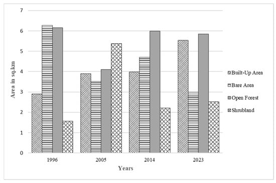
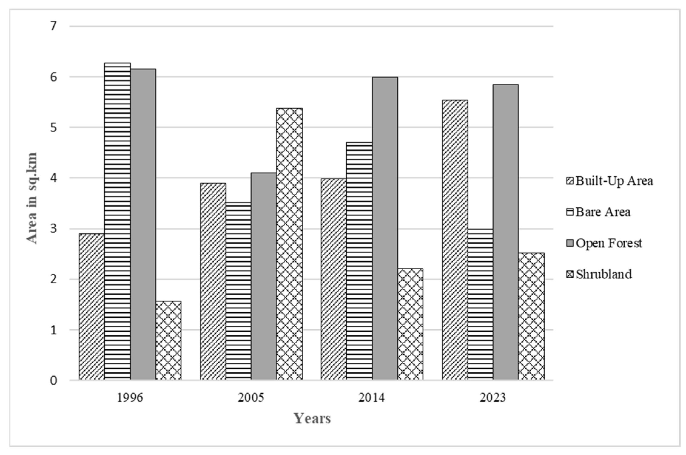
Figure 7 shows the changes in land cover areas from the years 1996 to 2023. The built-up area appeared to have a clear continuous increase over the years, with values 2.901 km2 in 1996 to 5.538 km2 in 2023. The built-up area covered 32.791% of the catchment during 2023. The bare area showed fluctuation values of 6.270 km2, 3.510 km2, 4.703 km2, and 2.990 km2. In 2023, it covered 17.705% of the catchment, contrasted with 37.122% in 1996. The open forest also showed minor fluctuation, with values of 6.148 km2, 4.105 km2, 5.997 km2, and 5.840 km2. In 2023, the open forest occupied 34.581% of the catchment, a slight reduction from 36.397% in 1996. Lastly, in the shrubland, it had values of 1.572 km2, 5.385 km2, 2.208 km2, and 2.520 km2, which also showed fluctuation results. It had a peak of 31.879% during 2005 and decreased to 14.922% during 2023. Hence, the data showed that the built-up area increased over the different time periods while the bare area decreased.
Figure 7.
Change of land cover areas from 1996 to 2023.
4.3. Hydrologic Modeling
4.3.1. Stage–Discharge Relationship
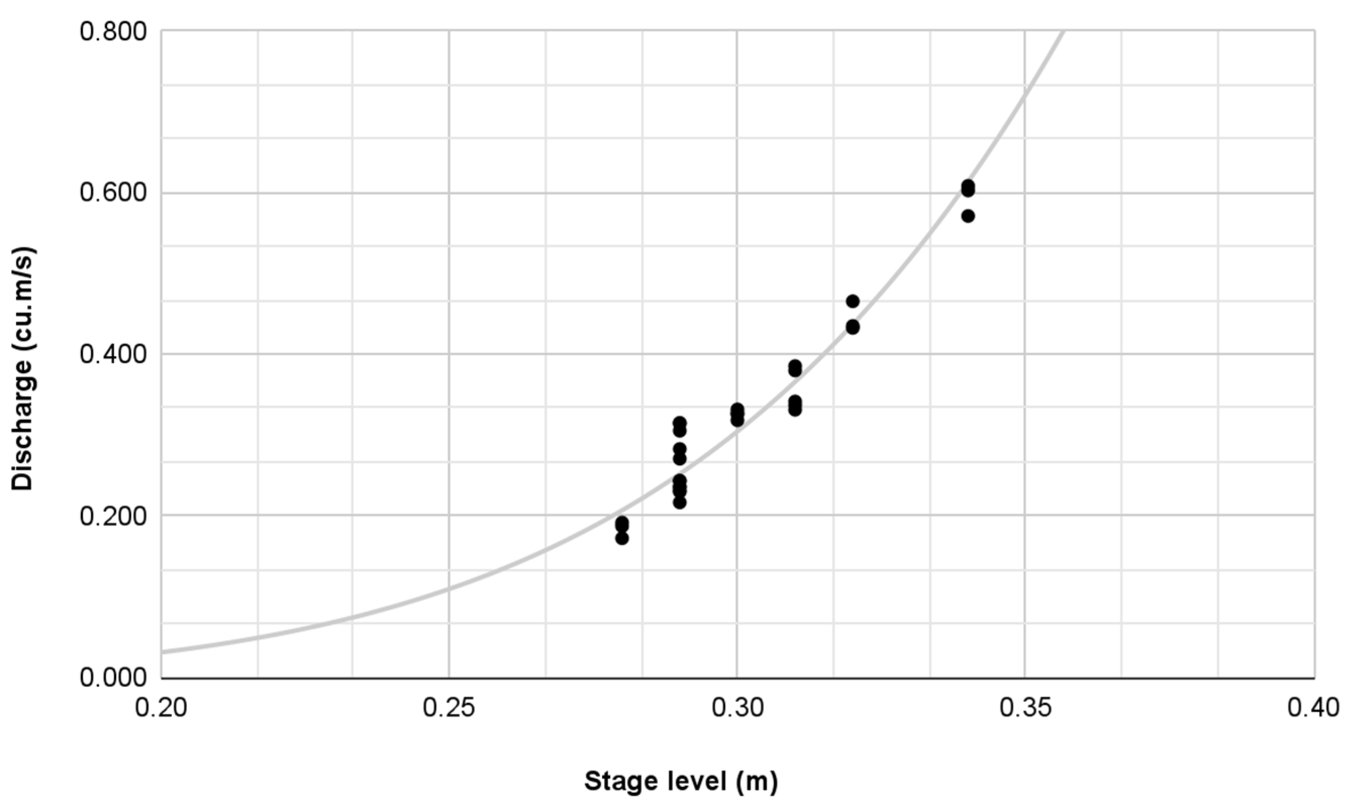
Based on 30 observed river velocity measurements, a rating curve was developed using the Power Law (Figure 8). The resulting rating curve equation was used to transform the observed stages into the corresponding discharges.
Figure 8.
Stage–discharge relationship at the outlet point.
4.3.2. HEC-HMS Model Calibration and Validation
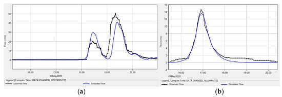
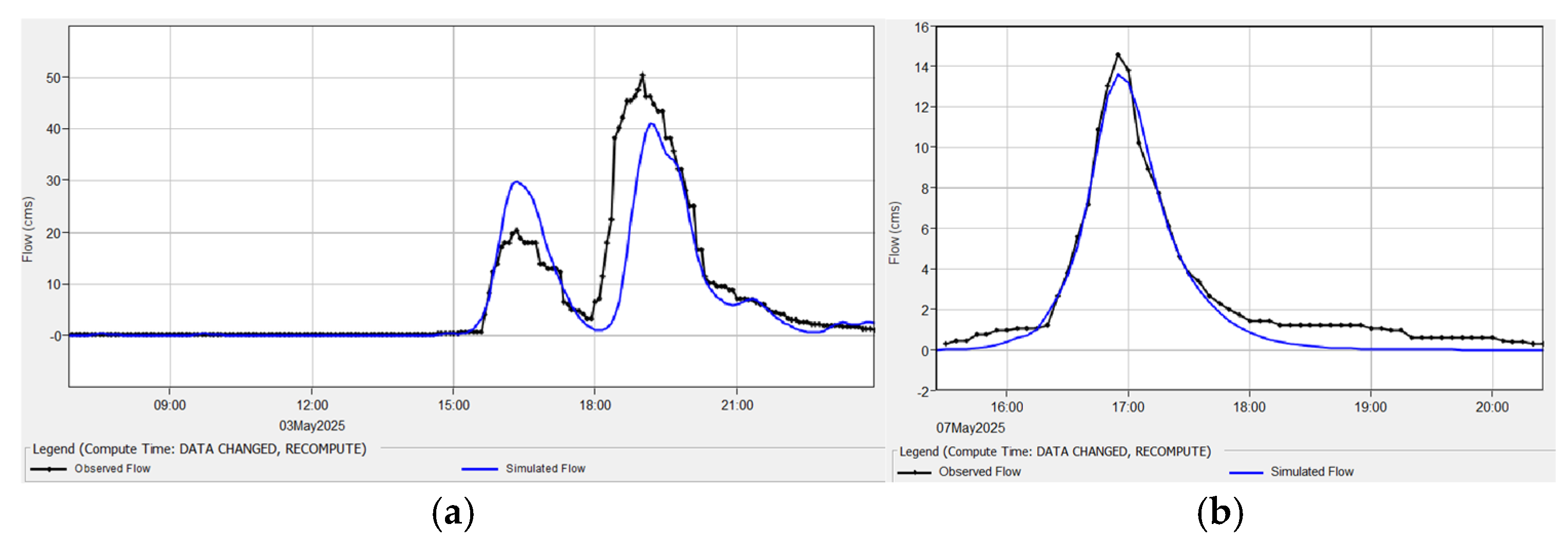
Model validation was performed using the independent storm event on 7 May 2025 (15:30 P.M. to 16:25 P.M) (Figure 9a). The simulated peak discharge was 13.6 m3/s against an observed discharge of 14.6 m3/s. The simulated runoff volume reached 39.1 × 10³ m3 compared to the observed runoff volume of 48 × 103 m3/s. Time to peak (Tp) was replicated precisely, with both simulated and observed peaks occurring at 16:55. The validation results demonstrated high fidelity (Figure 9b), achieving an NSE of 0.962, RSR is 0.20, and PBIAS is −18.77%. Goodness of fit for both events are summarized in Table 3 and Table 4.
Figure 9.
Observed hydrograph vs. simulated hydrograph during (a) calibration and (b) validation.
Table 3.
Model predictions and model performance rating after calibration.
Table 4.
Model predictions and model performance rating for model validation.
The hydrological model was calibrated using the rainfall and discharge data gathered from the rainfall event on 3 May 2025 with the rainfall time duration of 06:55 A.M. to 23:15 P.M. The calibrated model simulated a peak discharge of 41.1 m3/s and a runoff volume of 375.3 × 10³ m3. The simulated hydrograph peak time is 19:10. The calibrated model achieved an NSE of 0.755, RSR of 0.5, and PBIAS of −16.94%. These values indicate that the model’s performance is satisfactory and the simulated hydrograph provided a good fit with the observed hydrograph. The calibrated model was validated using the rainfall event on 7 May 2025 with the rainfall time duration of 15:30 P.M. to 16:25 P.M. The simulated peak discharge is 13.6 m3/s, which is lower than the observed discharge of 14.6 m3/s. The simulated runoff volume is 39.1 × 10³ m3 while the observed runoff volume is 48 × 103 m3/s. Additionally, the simulated time to peak occurred at 16:55, which is similar to the observed peak at 16:55. The validation results are satisfactory with an NSE coefficient is 0.962, RSR is 0.2, and PBIAS is −18.77%.
4.3.3. Runoff Simulations Across Return Periods
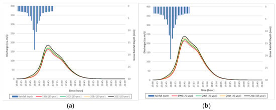
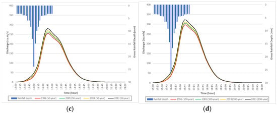
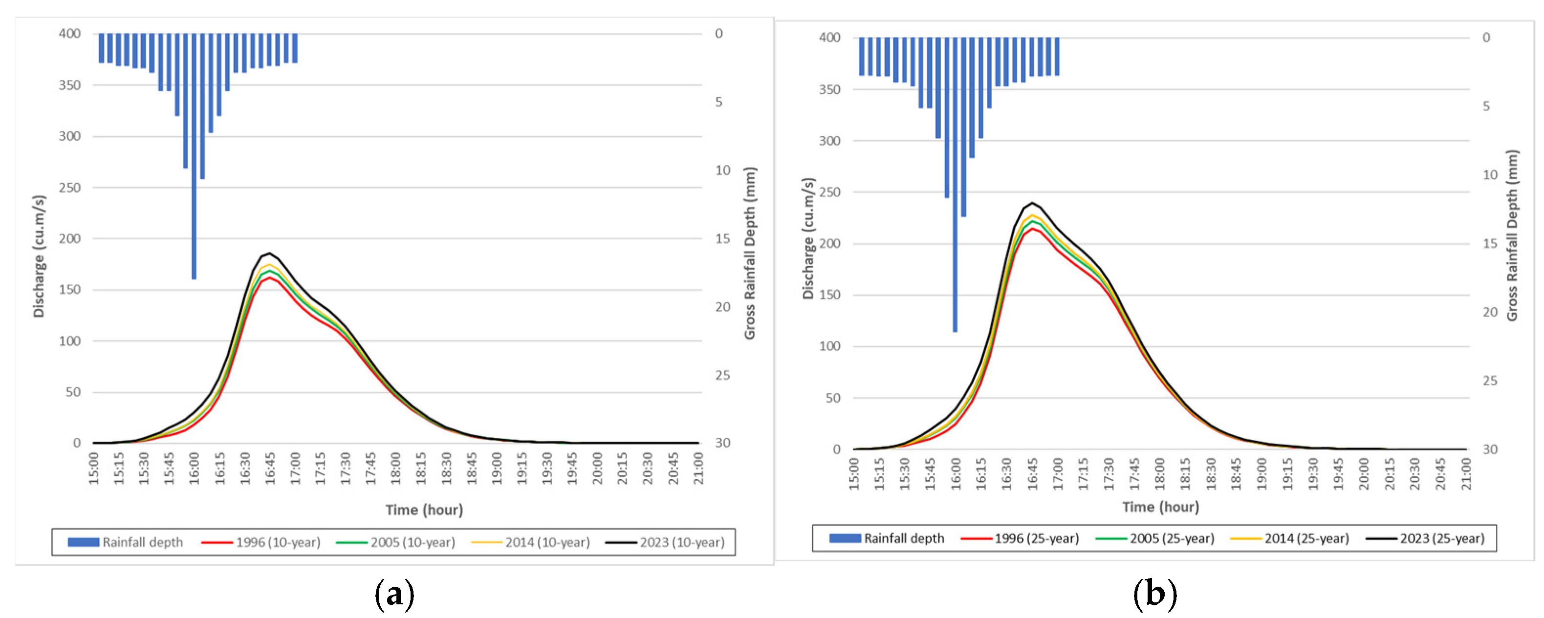
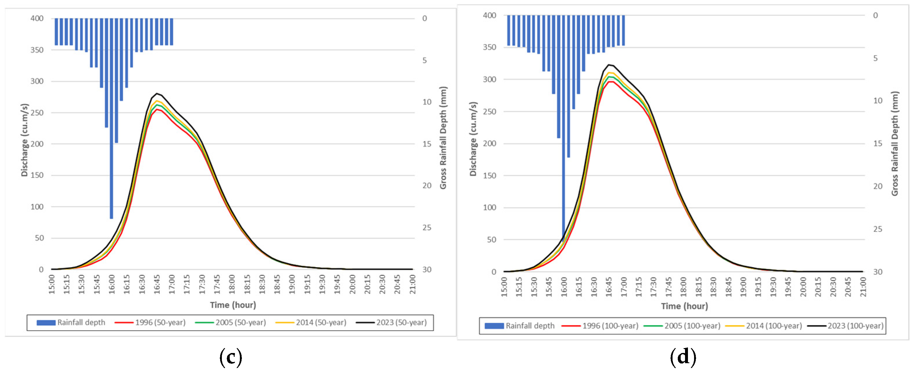
Scenario simulations using the validated HEC-HMS model revealed a consistent, monotonic increase in both peak discharge () and total runoff volume () across all evaluated return periods (-, -, -, and -year) from 1996 to 2023 (Figure 10). Adjusting subbasin SCS Curve Numbers () to reflect specific land cover configurations demonstrated that periods with rapid built-up expansion ( and ) corresponded to the highest percentage increases in peak discharge.
Figure 10.
Discharge hydrographs for (a) 10 yr, (b) 25 yr, (c) 50 yr, and (d) 100 yr storm return periods.
For example, under the -year storm scenario, simulated peak discharge at the basin outlet increased from 296.7 m3/s under 1996 land cover conditions to 322.7 m3/s under 2023 conditions, representing a net increase of [8.76%]. Similarly, total runoff volume expanded from 1656.1 × 103 m3 to 1825.5 × 103 m3 over the same period. Across all storm return periods and across all years, the hydrograph peak timing () remains constant because the same rainfall distribution pattern from the alternating block method was applied. Multi-scenario hydrologic simulation outputs are summarized in Table 5.
Table 5.
Percentage change of peak discharge and runoff volume.
4.4. Hydraulic Modeling
4.4.1. HEC-RAS 2D Model Calibration and Validation
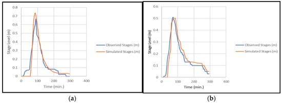
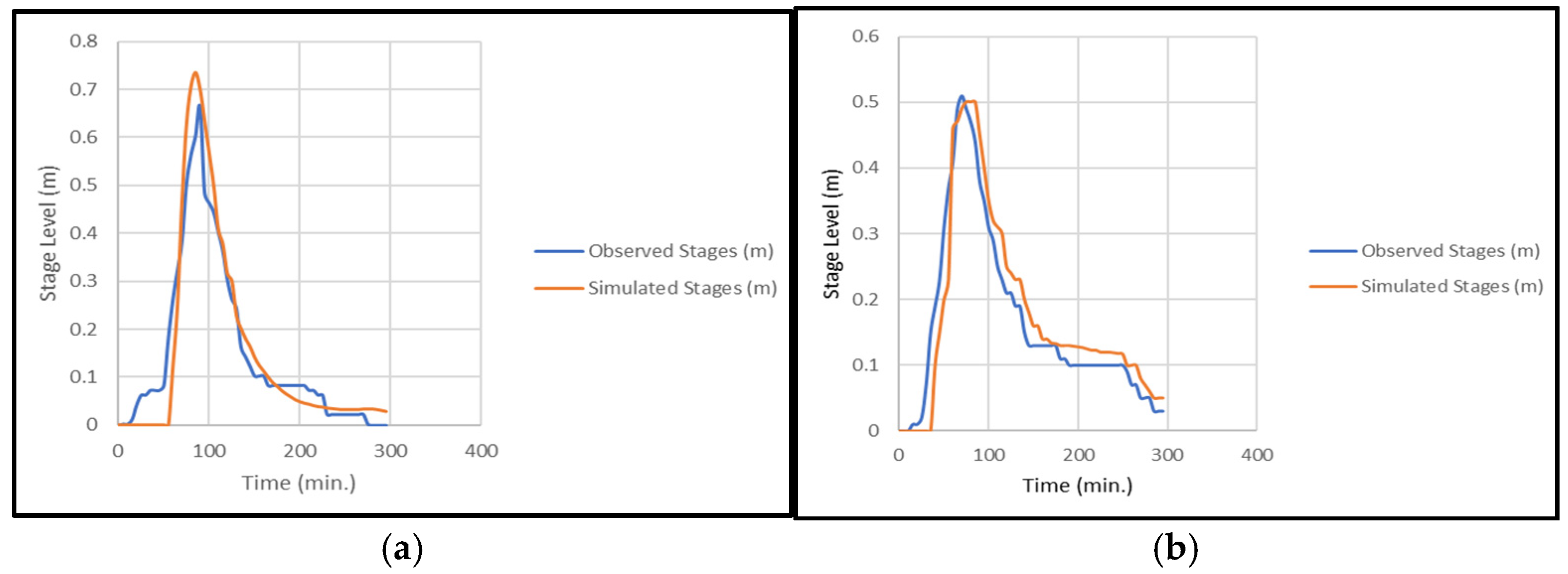
The 2D HEC-RAS model was calibrated by matching simulated stages with observed stages at the river outlet gauge (Figure 11a,b). Time series data was exported from RAS Mapper’s time series tools and compared to observations in Excel. Calibration was performed by adjusting Manning’s n roughness in channel and floodplain to match the stages. The main channel used n = 0.028 and overbanks n = 0.038. The calibration achieved an NSE of 0.88 and RMSE of 0.06. According to widely used hydrologic guidelines, NSE ≥ 0.75 indicates very good performance for streamflow/stage with a lower RMSE, which means the model reproduces the observed hydrograph well [24]. The calibrated hydraulic parameters (manning’s n, flow area, etc.) were kept and used to run a simulation of an independent rainfall event to test transferability. Model validation was then evaluated at the outlet by comparing water surface elevation (simulated stage) to observed stages. Using an independent event for validation follows hydrologic testing practice [29]. The validation event achieved an NSE of 0.89 and a RMSE of 0.05, which indicates good agreement and demonstrates that the calibrated roughness parameters work on an independent event.
Figure 11.
Observed vs. simulated stage hydrograph for (a) calibration, (b) validation.
4.4.2. Impact of Land Cover Change on Hydraulic Performance of Kinalumsan River
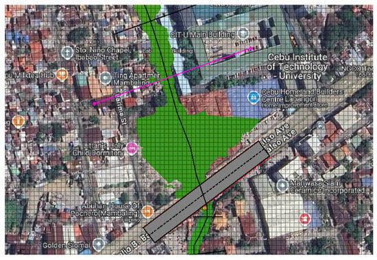
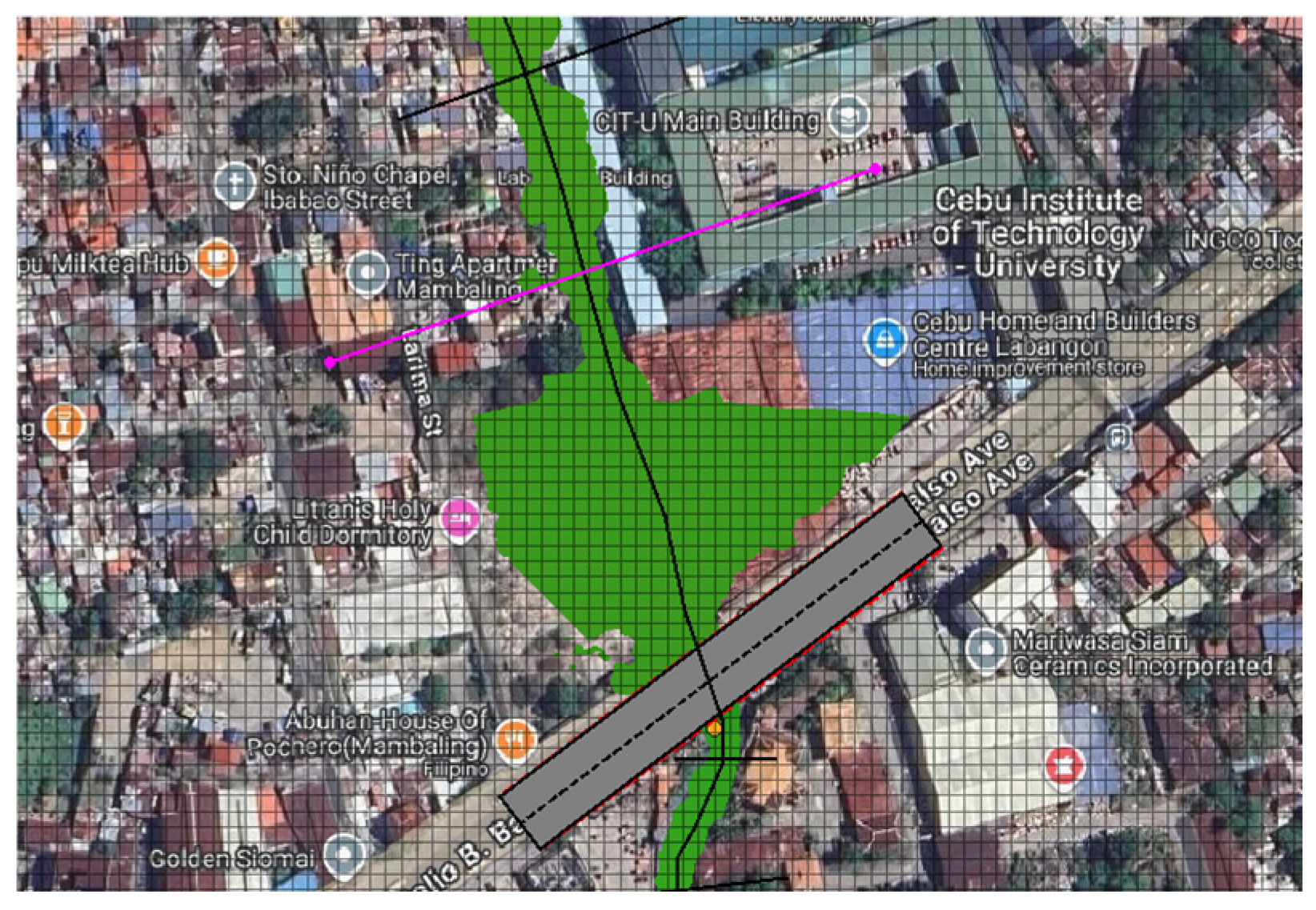
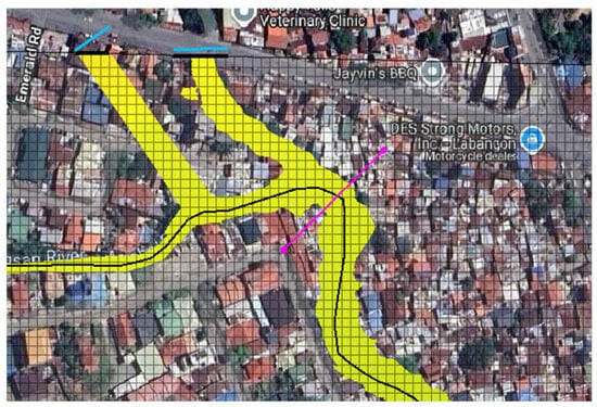
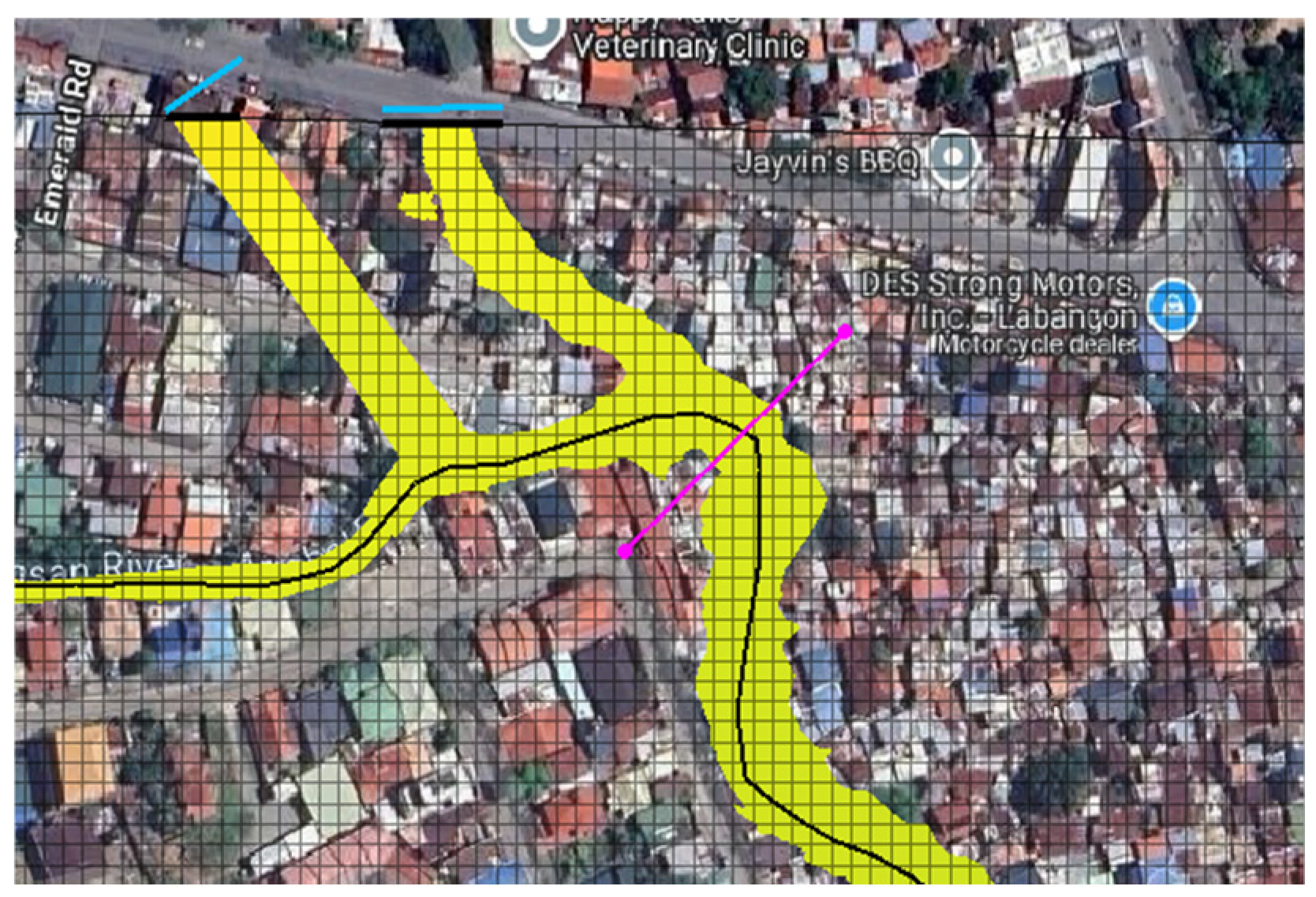
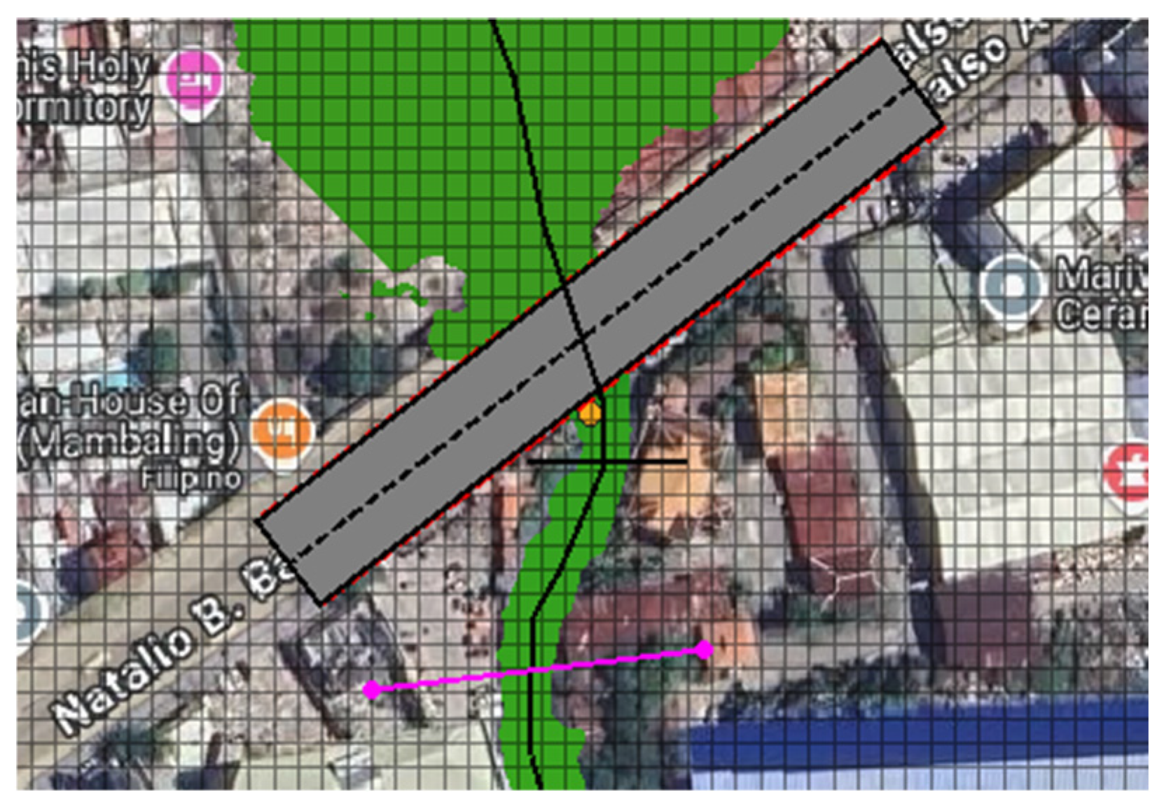
The assessment of the hydraulic performance of Kinalumsan river from 1996–2023 for various different return periods focuses on the hydraulic parameters such as discharge capacity, velocity, and hydraulic grade line. For each section, discharge capacity is defined as the flow of the water in the channel just as the water surface reaches the bank crest before spilling to the floodplain [30,31]. Capacity was extracted from model results using RAS profile lines (Figure 12, Figure 13 and Figure 14), where the flow right before the water surface reached the bank was determined in three key spots—the upstream, midstream and the downstream part of the river—as shown in Figure 8, Figure 9 and Figure 10.
Figure 12.
Upstream of Bridge (596,338.0941 E, 1,138,089.8694 N).
Figure 13.
After main tributaries (596,107.812 E, 1,138,633.089 N).
Figure 14.
Downstream of bridge (596,382.69 E, 1,137,933.63 N).
4.4.3. Impact of Land Cover Change on Urban Flooding
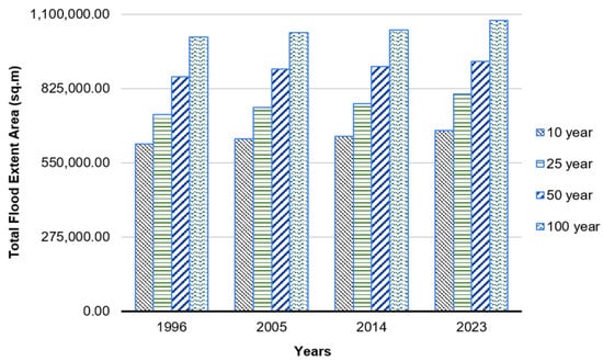
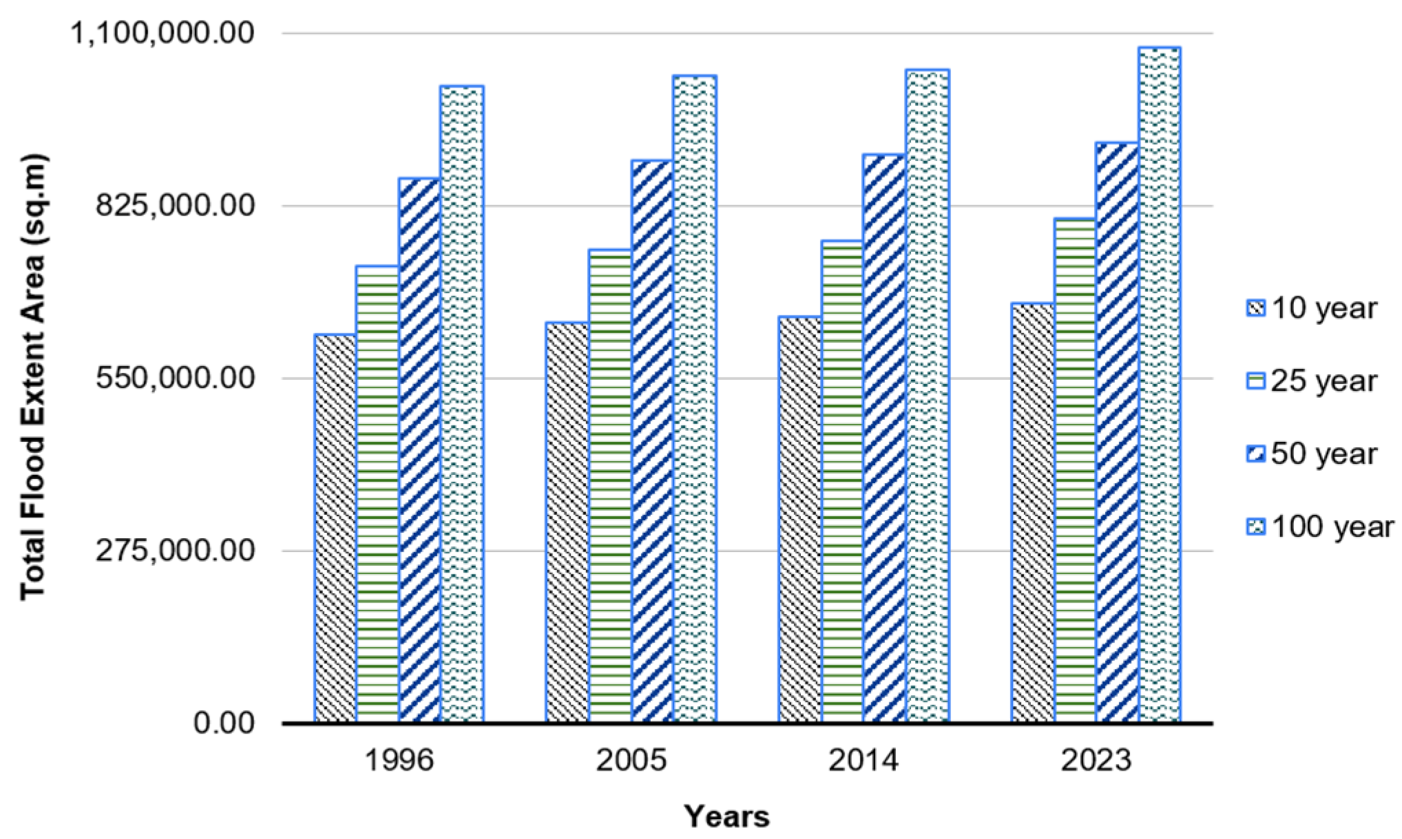
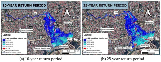
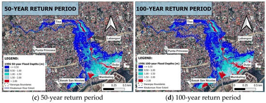
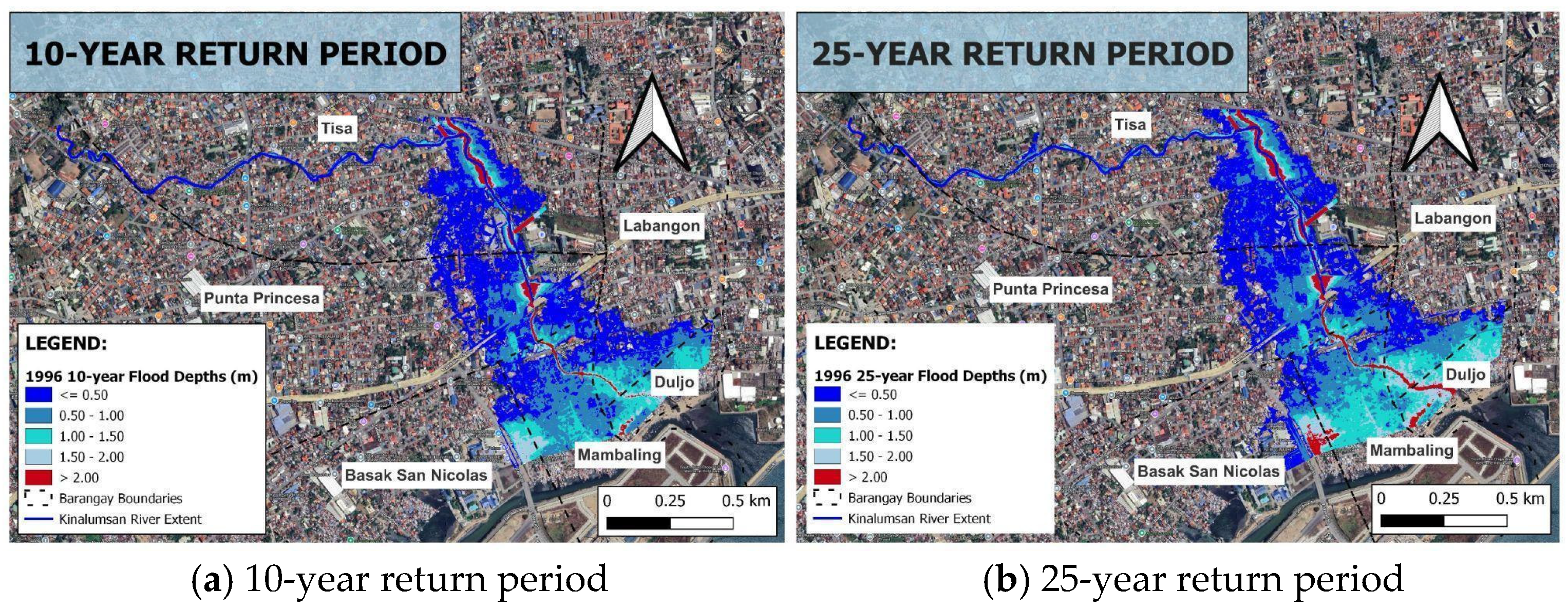
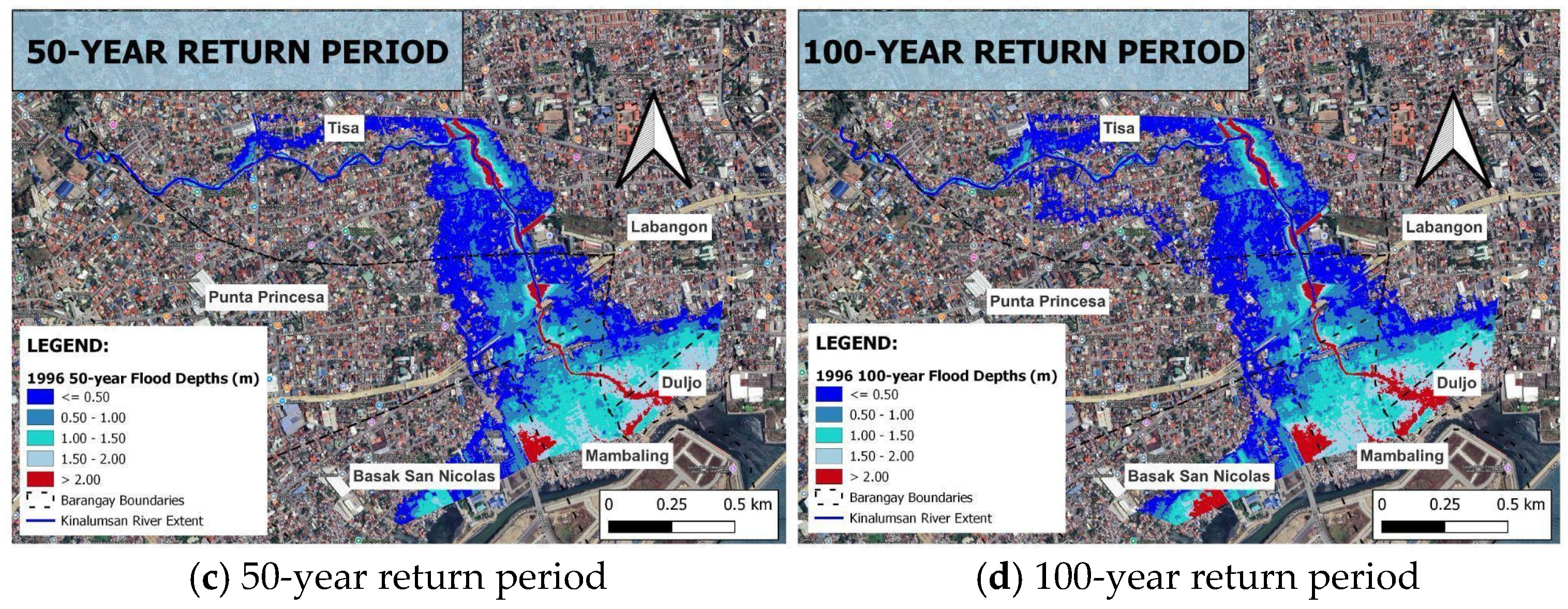
Figure 10 shows the simulated flood extent areas for 10-, 25-, 50-, and 100-year return periods. The results (Figure 15) reveal that the year 2023 exhibits the largest extent of flooded area for all the return periods, while 1996 shows the smallest extent of flooded areas. Flood extent areas increase consistently over time for each return period.
Figure 15.
Total area of simulated flood extents under different return periods.
In 1996, the total flooded area in Barangay Tisa increased consistently with higher return periods, increasing from 450,493 m2 under the 10-year event to 519,149 m2 for the 25-year, 602,142 m2 for the 50-year, and 668,913 m2 under the 100-year return period. A similar trend is observed in other years. In 2005, the total flooded area increased from 460,538 m2 for the 10-year event to 538,183 m2 for the 25-year event, 620,047 m2 for the 50-year event, and 678,116 m2 for the 100-year event. This trend persisted in 2014, with values increasing from 466,470 m2 in the 10-year event to 548,570 m2 in the 25-year event, 626,341 m2 in the 50-year event and 683,489 m2 in the 100-year event. By 2023, the flooded area further expanded, from 479,604 m2 in the 10-year event, to 578,209 m2 in the 25-year event, 642,690 m2 in the 50-year event, and 694,781 m2 in the 100-year event. While the individual barangays may not individually exceed Tisa in flooded areas, however, the aggregation of flooded areas from the barangays located at the downstream portion results in an area far larger than that of Barangay Tisa as seen in Table 6.
Table 6.
Area of flooding extents for barangays near the downstream portion of the Kinalumsan River in Cebu City, Philippines.
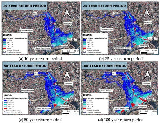
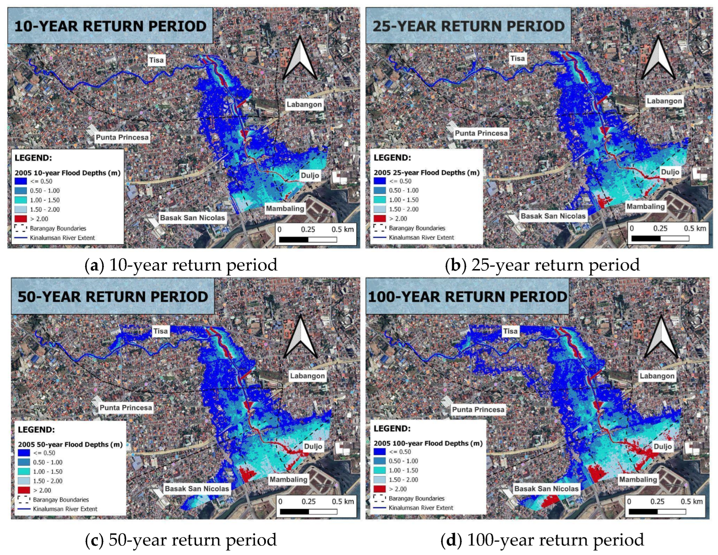
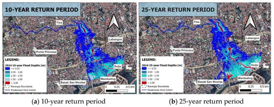
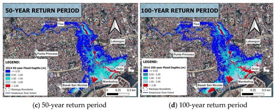
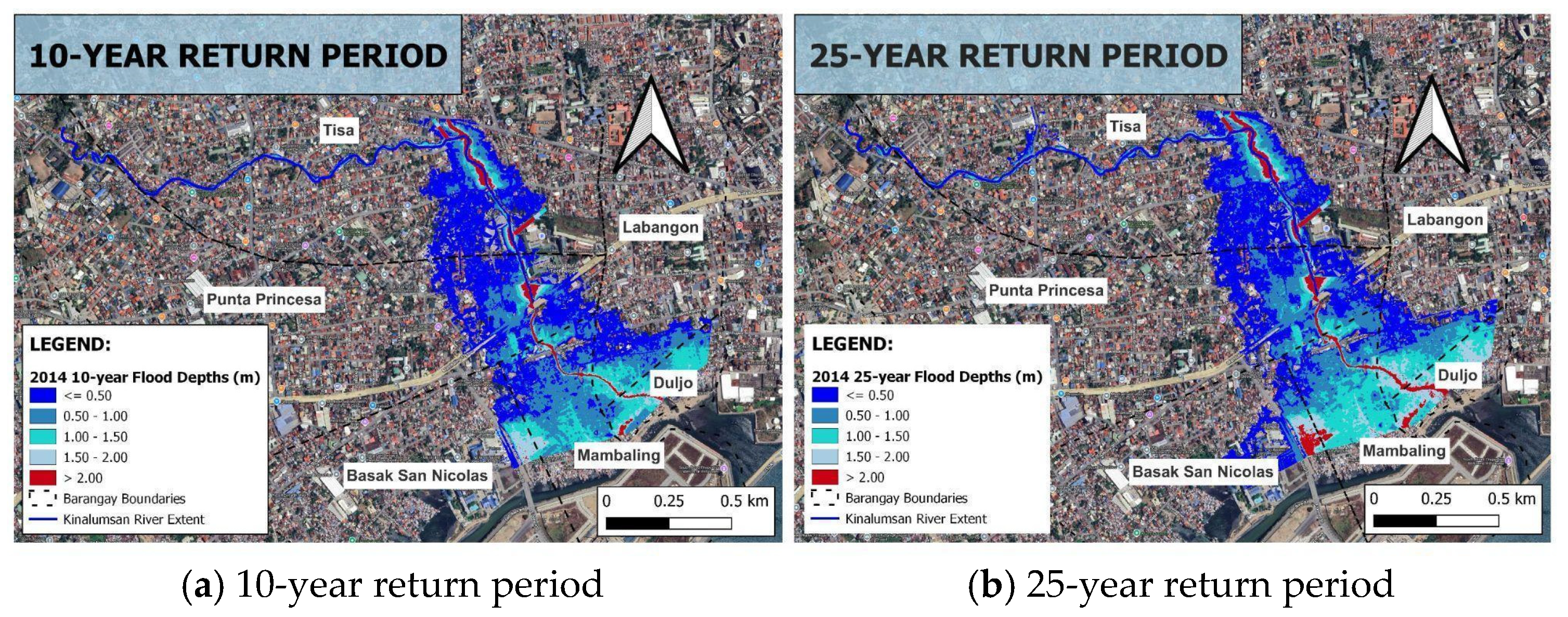
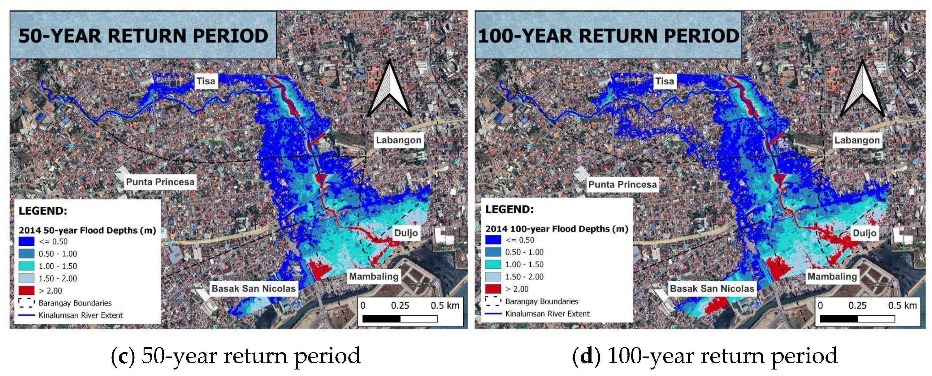
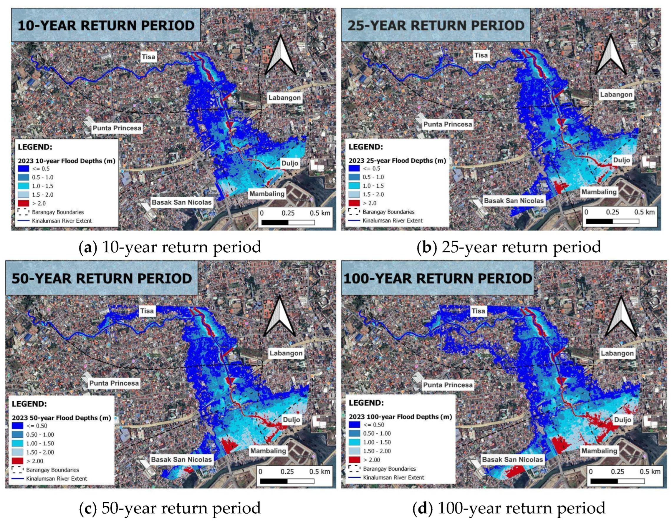
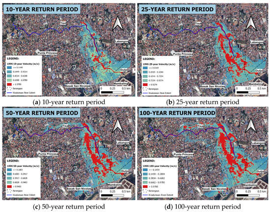
For every year, the corresponding affected area (in m2) is quantified per flood depth class. Across all years, the increase in depth is not uniform for various depth classes (Figure 16, Figure 17, Figure 18 and Figure 19). Deeper categories scale much more with event size. The barangay-specific trends show that certain areas consistently bear the brunt of deeper flooding under extreme events. Tisa consistently contributes the widest flooded area, dominated by the shallow depth class (0.0–0.5 m), followed by Punta Princesa (Figure 16). In contrast, the barangays of Mambaling and Duljo Fatima are mainly concentrated by deeper classes (≥1.5 m and ≥2.0 m), highlighting their vulnerability to catastrophic flooding. Punta Princesa and Labangon remain dominated by shallow to moderate flood depths across all return periods. Mambaling exhibits pronounced gains in the deeper classes, particularly under the 50- and 100-year events, indicating that flood severity is expanding into them more than into barangays with lower base exposure. Meanwhile, Basak San Nicolas shows the smallest increments in deeper depth classes, implying that much of its flood exposure remains in the lower depth bands.
Figure 16.
Flood inundation depth maps generated for the 1996 under four extreme rainfall scenarios.
Figure 17.
Flood inundation depth maps generated for the 2005 under four extreme rainfall scenarios.
Figure 18.
Flood inundation depth maps generated for the 2014 under four extreme rainfall scenarios (a–d).
Figure 19.
Flood inundation depth maps generated for the 2023 under four extreme rainfall scenarios (a–d).
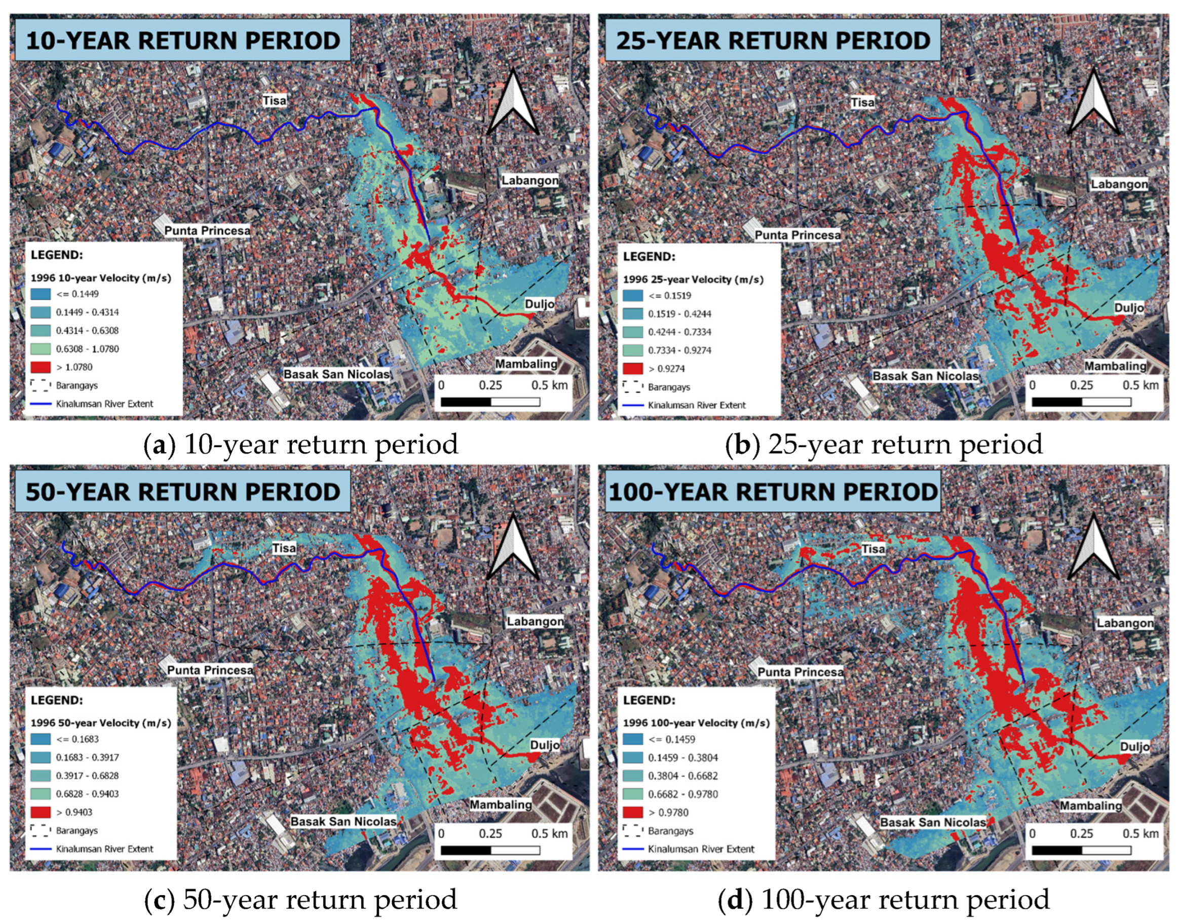
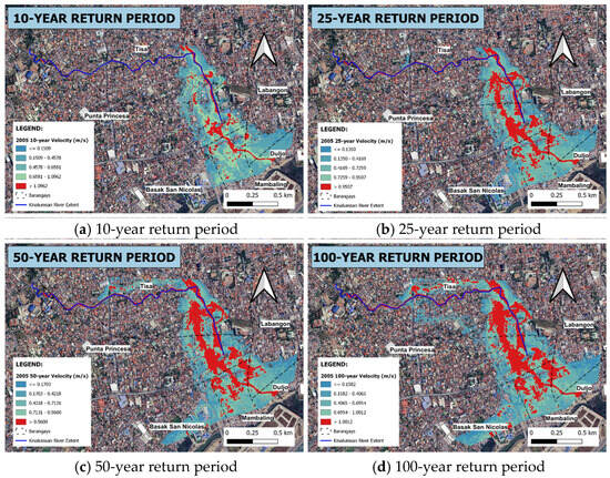
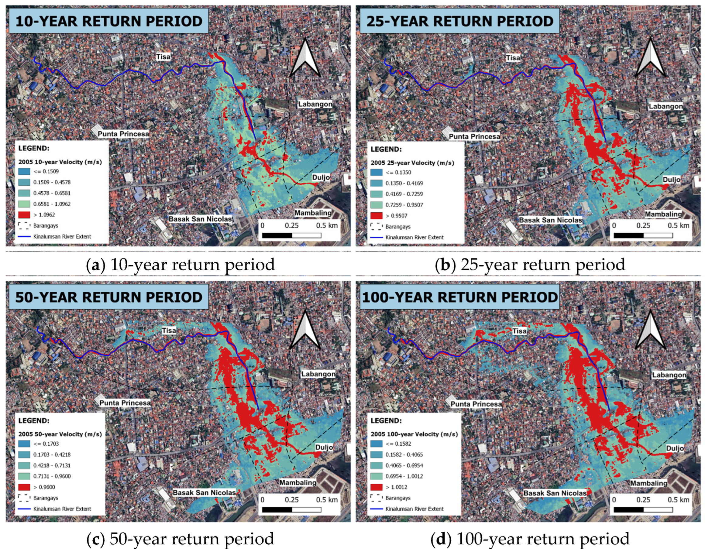
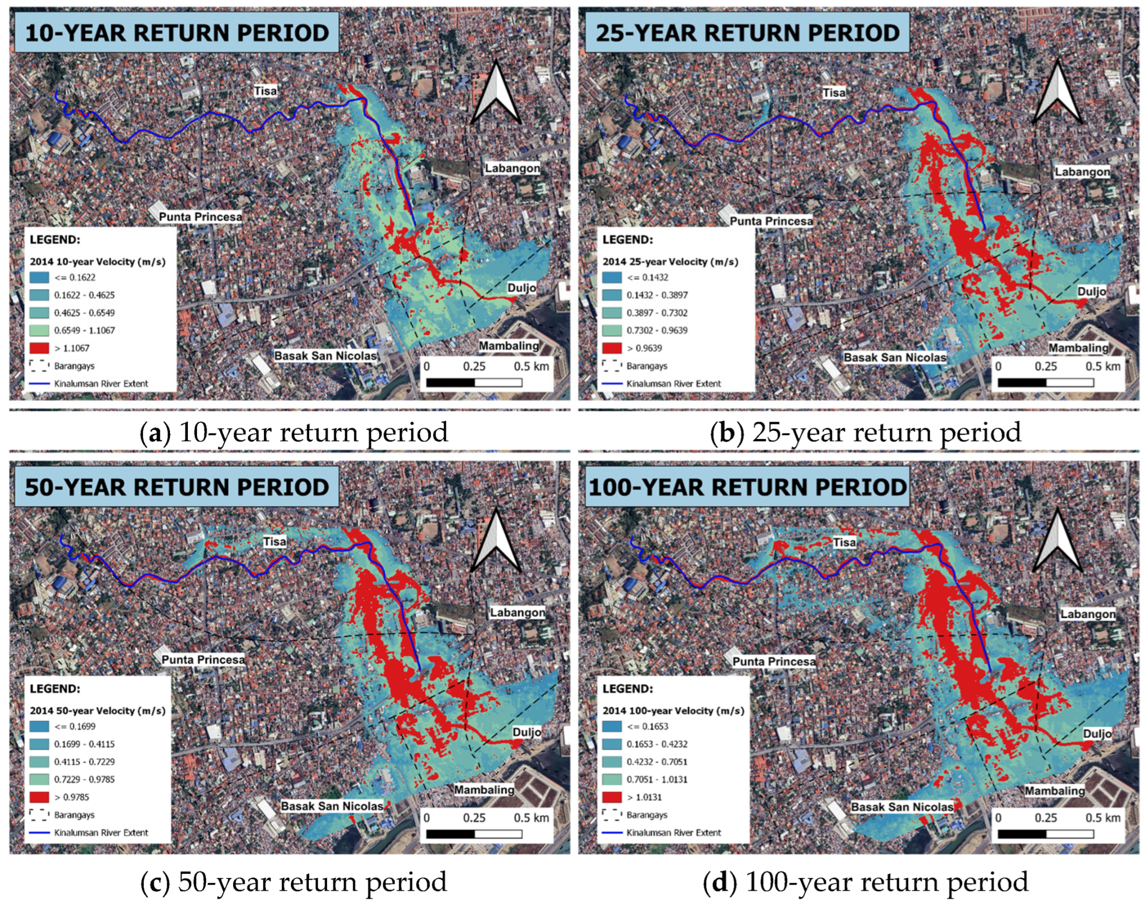
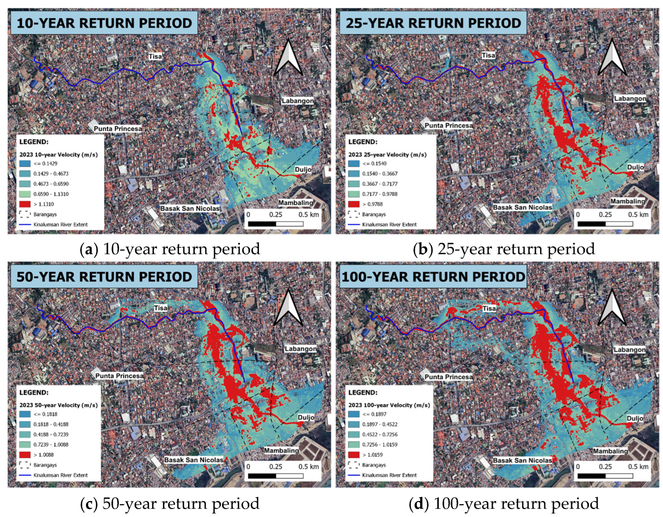
From the flood velocity maps (Figure 20, Figure 21, Figure 22 and Figure 23), Tisa consistently has one of the largest affected areas, but with the lowest velocity class (0.0–0.6 m/s). This suggests that a large portion of Tisa lies within shallow, slow-moving flood zones. The barangay also shows significant area in higher velocity classes, which implies that parts of Tisa are closer to stronger flow paths, exposed to more energetic flow under higher return periods. In contrast, Basak San Nicolas tends to have relatively modest area counts in the higher velocity classes. For example, the affected area in >2.4 m/s is nearly zero or very small in this barangay. This suggests Basak is less frequently subjected to high-velocity flows, possibly being more removed from core flow corridors. Punta Princesa and Mambaling often show intermediate behavior: moderate area in low velocity, but also non-negligible area in the 0.6–1.2 m/s and 1.2–1.8 m/s classes for larger return periods. This suggests that these barangays are sometimes exposed to faster flows depending on flood magnitude. Duljo Fatima also shows exposure to higher velocity classes, though in smaller magnitudes than Tisa or Mambaling. Its value in mid- and higher velocity grows more noticeable in extreme return periods, indicating that under strong flows, flow encroaches into Duljo Fatima.
Figure 20.
Flood velocity maps generated for the 1996 under four extreme rainfall scenarios (a–d).
Figure 21.
Flood velocity maps generated for the 2005 under four extreme rainfall scenarios (a–d).
Figure 22.
Flood velocity maps generated for the 2014 under four extreme rainfall scenarios (a–d).
Figure 23.
Flood velocity maps generated for the 2023 under four extreme rainfall scenarios (a–d).
5. Discussion
5.1. Impact of Land Cover Change
The continuous expansion of built-up surfaces from 32.79% in 1996 to in 2023, coupled with a noticeable decline in natural bare ground, represents a major structural shift in the hydrological response of the Kinalumsan catchment. Physically, replacing permeable soil matrixes with impervious asphalt and concrete alters the catchment’s water balance by reducing initial abstraction () and infiltration capacity.
These results line up with findings from Ongaga et al. (2024) [32], who utilized Landsat data and HEC-HMS to present how increasing impervious surface with increased modeled runoff. In Kinalumsan, the expansion of built-up areas directly increased the amount of rainfall turning into surface runoff.
Within the HEC-HMS modeling framework, this structural shift directly dictates the composite SCS Curve Number (). As built-up coverage expands, weighted values increase across the subbasins, causing a greater fraction of effective rainfall to convert directly into surface runoff rather than percolating into ground storage. Furthermore, the smooth surfaces of dense urban development reduce hydraulic roughness, accelerating overland flow velocities. This severely shortens the Time of Concentration () and catchment lag time (), transforming the basin into a “flashy” system characterized by steep hydrograph rising limbs and elevated peak discharges ().
These findings align closely with observations in similar rapidly urbanizing tropical catchments [33], where anthropogenic land cover transitions systematically outpaced the conveyance capacity of historical drainage networks, exacerbating localized flash inundation.
Cumulative Hydrological Impacts of Long-Term Urbanization
The multi-temporal scenario simulations illustrate how historical LULC alterations directly increase flood risk across varying storm frequencies. The strong alignment between periods of rapid built-up expansion ( and ) and elevated percentage gains in confirms that urbanization is the primary driver of hydrologic change in the Kinalumsan catchment.
Physically, replacing natural cover with impervious surfaces reduces catchment storage, forcing higher composite values. This structural alteration shifts the rainfall–runoff relationship, causing even moderate, low-return-period rainfall events under 2023 conditions to generate peak flows that match or exceed those produced by larger design storms under 1996 conditions. This trend closely aligns with the findings of Supratman et al. [34], who observed that changes in land use and cover were associated with increased peak flood flow of the Mampang river and increased flood risk areas using HEC-HMS and HEC-RAS. The result suggests that continued urbanization can progressively increase runoff response even when the rainfall scenario is held constant for comparison.
These simulated trends demonstrate that ongoing unmanaged urbanization will progressively compress flood response windows, leaving downstream communities increasingly vulnerable to flash inundation during high-return-period storms [33].
5.2. Hydraulic Performance of the Kinalumsan River
The HEC-RAS results seen in Table A10 show that the simulated peak discharge exceeds the discharge capacity in all river segments presented. It is important to note that discharge capacity being referred here pertains to the capacity of the river to carry water within its banks and does not account for the capacity of the floodplains once the banks are flooded or overtopped by river water. Floodplain capacity was not considered as most of it is occupied already by residential and commercial buildings.
Additionally, results reveal that the water surface elevation (WSE) remains consistently higher than the terrain profile across all the years considered. The water surface elevation increases with stronger return periods. The average depth above the river bed varies between 2 and 5 m. The hydraulic grade line (HGL) observed between the years studied and return periods considered changed by an average of around 0.7 m. For example, station 2050 of the 50-year return period, there was a WSE of 8.72 m in 1996, 9.28 m in 2005, 9.63 m in 2014 and 9.83 m in 2023. This averages a change of 0.4 m and is expected since water rises to the same level before spilling to the floodplain, resulting in a small rise in the water surface elevation in the channel [35,36]. Noticeable changes in HGL at stations 750, 2000, and 2500 were observed for each year which is primarily due to the presence of bridges. Bridges constrict the flow through the channel, causing the water level upstream to rise (backwater rise) and build up potential energy needed to accelerate the flow through the channel [37]. This often results in river overflows causing flooding in its surrounding areas.
The bridge-related changes therefore indicate that flood risk is concentrated at specific hydraulic bottlenecks rather than being controlled only by the overall increase in runoff. Khan et al. [38] correspondingly demonstrated the usage of HEC-RAS 2D and ArcGIS for assessing the flood depth, extent, and velocity under various return periods. These bridge sections are essentially priority areas for Kinalumsan’s inspection and maintenance.
5.2.1. Flood Inundation Characteristics
The extent of the areas flooded increases with higher return periods, indicating the impact of more intense rainfall events. The simulation results (Figure 11, Figure 12, Figure 13 and Figure 14) reveal that Barangay Tisa consistently exhibits the largest flooded area among all the barangays; however, when the ratio of the flooded area to the barangay areas are considered, Duljo Fatima ranks first in terms of inundation with about 59–60% of its land area affected floods under all scenarios.
Overall, these trends suggest that as flood intensity increases, not only does inundation expand laterally, but the high-risk zones deepen and concentrate in already vulnerable barangays. Additionally, a significant positive correlation is observed, indicating that as the imperviousness of the catchment increases, the flood volume also increases.
The relationship between land cover changes and flood hazard is consistent with Supratman et al. [34], where changes in peak flow and flood risk areas accompanied increasing urban land cover. This supports interpreting the Kinalumsan inundation results as a combined effect of increased runoff and the river system’s limited flow capacity.
5.2.2. Flood Velocity
Across all scenarios as seen in Figure 15, Figure 16, Figure 17 and Figure 18, the highest velocities are mainly along the main channel, especially at bends and near bridges, while newly inundated flood cells remain slower. This spatial pattern is expected as HEC-RAS 2D routes flow by solving the shallow water equations over the mesh, and open channel velocity scales with hydraulic radius and slope per Manning’s relation [38,39]. This means that where it is steeper and smoother, HEC RAS simulates water movement from cell to cell faster, and if it is shallow and rougher, or at narrowings like bridges, water accelerates as it contracts and expands. With increasing event severity from 10-year return period to 100-year return period, the inundation spreads and the area of moderate velocities grow, while the peak velocities remain largely unchanged but in the same area. The fast velocities are consistent in the channel and shallow at the overbank.
Over time, it can be seen that velocity exposure expands. More area in barangays moves from the lower velocity classes into mid or higher velocity as return period increases. For example, the >2.4 m/s class, which is almost absent in 10-year events, appears more in 100-year events. That shows that for heavy flows, more barangays are forced into harsher hydraulic conditions. Overall, the barangays differ in vulnerability to flow velocity. Tisa appears most exposed, Basak San Nicolas is the least, and other barangays fall in between. The progression of velocity exposure with increasing flood severity suggests that under extreme events, even barangays under mild floods could be affected by higher flows. These insights are valuable for prioritizing flood mitigation and emergency planning according to velocity risk, not just depth.
This finding is in line with Ullah et al. [37], who emphasized that evaluating flow velocity alongside inundation depth provides a far more complete picture of spatial flood hazard. Similarly, this study shows that the fastest flows stay confined to main channels and bottlenecks, but heavier rainfall pushes much larger areas into moderate and high-risk zones. This makes it clear that emergency planners and local officials need to account for water velocity—not just flood depth—when preparing for severe storms.
5.3. Study Limitations and Model Scope
A primary operation constraint of this study is its reliance on a discrete, event-based monitoring dataset collected during a short-term field campaign in an ungauged catchment. While discrete event calibration establishes baseline physical parameters (CN, Tc) and replicates hydrograph timing with high fidelity (NSE = 0.962), caution must be exercised when extrapolating these parameters to extreme, high-return-period synthetic storms. Severe storm vents may trigger different catchment responses, variable antecedent moisture conditions, and floodplain roughness changes not fully captured during moderate operational events. Consequently, the current coupled HEC-HMS/HEC-RAS model should be viewed as an initial, expandable baseline framework. Additionally, due to resource constraints, model calibration in this study relied on a short-term (2–3 month) monitoring campaign capturing low-to-moderate flow events. While this provided a necessary baseline for first-order flood hazard mapping, future iterations of this model would benefit significantly from an extended multi-season monitoring period. Long-term streamflow records using automated pressure transducers or radar-based velocity meters will allow for rigorous multi-event calibration and a formal parameter sensitivity analysis, further reducing predictive uncertainty for high-return period extreme events.
Future research should focus on expanding the local hydrometric monitoring network to capture a wide spectrum of storm intensities for continuous model re-calibration. The results also have practical implications for flood management. While land use and stormwater measures that lessen effective imperviousness can enhance structural controls, sections close to bridges and other places where simulated discharge surpassed channel capacity should be given priority for regular channel clearing and structural checks.
6. Conclusions
The classified land cover maps for the years 1996, 2005, 2014, and 2023 achieved overall accuracies of 85.003%, 91.8171%, 86.33%, and 92.81%, respectively. Analysis of these maps revealed that the built-up areas are increasing at a rate of 4.332% annually, with the biggest spike recorded between 2014 and 2023.
A HEC-HMS rainfall–runoff model was developed to assess how land cover changes affect the Kinalumsan River’s discharge and runoff volume across 10-, 25-, 50-, and 100-year return periods. Calibration and validation statistical metrics confirmed satisfactory model performance in simulating the catchment’s hydrologic response. Results reveal that expanding built-up areas consistently increases peak discharge and runoff volume, highlighting a growing flood risk without proper mitigation. A 2D HEC-RAS model was developed to evaluate the hydraulic capacity, flood depths, extents, and velocities of the Kinalumsan River under extreme rainfall events from 1996 to 2023. Manning’s roughness coefficients were calibrated to for the main channel and for the floodplains, matching simulated stages with observed water levels. The model achieved high reliability, yielding strong calibration and validation scores ( and , respectively) that confirm close alignment with observed hydrographs.
A barangay-level analysis revealed that Tisa and Punta Princesa face the greatest initial exposure to extreme flood depths and high-velocity flows during lower return periods. As storm intensity scales up, deep flooding progressively shifts toward downstream areas like Mambaling and Duljo Fatima, with maximum flows overtopping channel capacities across several river profiles. Ultimately, these spatial shifts demonstrate that land cover changes not only expand overall flood extents but actively reframe localized risk profiles for depth and velocity hazards.
7. Recommendations
Based on the findings of the study, the researchers recommend the prioritization of channel maintenance at/near bridges since the controlling capacity is typically located there. To generate a more complete rating curve, future researchers are recommended to collect streamflow measurements during medium and higher flow conditions. Higher-stage data would reduce uncertainty in estimating discharge during extreme events and enhance the hydraulic modeling’s accuracy. Additionally, the inclusion of tidal fluctuations into the simulation would help improve the robustness of the model as it can influence downstream boundary conditions, water surface elevations and backwater effects, particularly in low-lying coastal reaches. It is suggested that pairing urbanization of areas along with nature-based solutions to counter the simulated rise in imperviousness and associated peaks/volumes be performed. Future researchers are encouraged to investigate alternative flood mitigation measures—such as the use of structural solutions like retention ponds, detention basins, or green infrastructure—and assess their effectiveness in reducing peak flows in the catchment. This simplified and cost-effective method of flood modelling can be upscaled to other cities where data is scarce, including the selection of nature-based solutions for the improvement of urban drainage and stormwater management for resilient cities.
Author Contributions
Conceptualization, N.A.K.R., F.B., A.B.C. and K.M.M.B.; Methodology, N.A.K.R., T.M.A.B., A.M.I.A., A.B.C. and K.M.M.B.; Software, T.M.A.B. and A.M.I.A.; Validation, T.M.A.B., A.M.I.A. and K.M.M.B.; Formal analysis, T.M.A.B., A.M.I.A. and A.B.C.; Investigation, T.M.A.B. and A.M.I.A.; Resources, A.B.C.; Data curation, T.M.A.B., A.M.I.A., A.B.C. and K.M.M.B.; Writing—original draft, T.M.A.B., A.M.I.A. and K.M.M.B.; Writing—review and editing, F.B. and K.M.M.B.; Visualization, T.M.A.B. and A.M.I.A.; Supervision, F.B. and A.B.C.; Project administration, A.B.C. All authors have read and agreed to the published version of the manuscript.
Funding
This research received no external funding.
Data Availability Statement
State weather agency’s (PAGASA) data on the rainfall intensity duration frequency cannot be shared due to a signed agreement. It can, however, be requested from the weather state agency in writing. Primary data used by the authors such as rainfall data and stream flow data cannot be made available due to a signed nondisclosure agreement but it can, however, be requested from the corresponding authors.
Acknowledgments
Appreciation is likewise given to the USC Civil Engineering Department Laboratory for providing equipment and technical assistance, and to the Office of the Barangay Mambaling in Cebu City, Philippines for granting permission to conduct data collection.
Conflicts of Interest
The authors declare no conflict of interest.
Abbreviations
The following abbreviations are used in this manuscript:
| PAGASA | Philippine Atmospheric, Geophysical and Astronomical Services Administration |
| GIS | Geographic Information System |
| DEM | Digital Elevation Model |
| HEC-HMS | Hydrologic Engineering Center’s Hydrologic Modeling System |
| HEC-RAS | Hydrologic Engineering Center’s River Analysis System |
| LiPAD | LiDAR Portal for Archiving and Distribution |
| LULC | Land Use Land Cover |
| SCS CN | Soil Conservation Service Curve Number |
| SCS UH | SCS Unit Hydrograph |
Appendix A
This section shows the model parameters used during HEC-HMS simulations.
Table A1.
Parameters for the routing method.
Table A2.
Routing method parameter values for calibration.
Table A3.
HEC-HMS model parameters for 2023 simulation before and after calibration.
Table A4.
Final model parameters used for each year.
Appendix B
The total area for each land cover classification and their corresponding computed discharge capacity and flood area extent are tabulated in this section.
Table A5.
Area of each land cover class from 1996 to 2023.
Table A6.
1996 land cover accuracy assessment.
Table A7.
2005 land cover accuracy assessment.
Table A8.
2014 land cover accuracy assessment.
Table A9.
2023 land cover accuracy assessment.
Table A10.
Discharge capacity.
Table A11.
Total area of simulated flood extents under different return periods.
References and Note
- Duan, Y.; Xiong, J.; Cheng, W.; Li, Y.; Wang, N.; Shen, G.; Yang, J. Increasing Global Flood Risk in 2005–2020 from a Multi-Scale Perspective. Remote Sens. 2022, 14, 5551. [Google Scholar] [CrossRef] [Scilit]
- World Meteorological Organization (WMO). Climate Change and Extreme Weather Impacts Hit Asia Hard; World Meteorological Organization (WMO): Geneva, Switzerland, 2024. [Google Scholar]
- PAGASA. About Tropical Cyclones; PAGASA: Quezon City, Philippines, 2022. Available online: https://dost.gov.ph/ (accessed on 19 July 2026).
- Alcantara, J.; Fellow, P.; Christopher, J. Briefing Note Regional Fellowship Program Overview of the Societal Impacts of Floods in the Philippines. 2019.
- United Nations Department of Economic and Social Affairs. World Urbanization Prospects The 2018 Revision; United Nations: New York, NY, USA, 2018. [Google Scholar]
- PSA. Highlights of the 2010 Census-Based Population Projections; Philippine Statistics Authority: Quezon City, Philippines, 2016. [Google Scholar]
- Miller, J.D.; Kim, H.; Kjeldsen, T.R.; Packman, J.; Grebby, S.; Dearden, R. Assessing the Impact of Urbanization on Storm Runoff in a Peri-Urban Catchment Using Historical Change in Impervious Cover. J. Hydrol. 2014, 515, 59–70. [Google Scholar] [CrossRef] [Scilit]
- Borgonia, K.M.M.; Fornis, R.L. Estimation of the Reduction in Flood Peak and Flood Volume Due to Rooftop Rainwater Harvesting for Nonpotable Use. In Proceedings of the AIP Conference Proceedings; AIP Publishing LLC: New York, NY, USA, 2020; Volume 2278. [Google Scholar]
- Omurakunova, G.; Bao, A.; Xu, W.; Duulatov, E.; Jiang, L.; Cai, P.; Abdullaev, F.; Nzabarinda, V.; Durdiev, K.; Baiseitova, M. Expansion of Impervious Surfaces and Their Driving Forces in Highly Urbanized Cities in Kyrgyzstan. Int. J. Environ. Res. Public Health 2020, 17, 362. [Google Scholar] [CrossRef] [Scilit] [PubMed]
- Hrachowitz, M.; Savenije, H.H.G.; Blöschl, G.; McDonnell, J.J.; Sivapalan, M.; Pomeroy, J.W.; Arheimer, B.; Blume, T.; Clark, M.P.; Ehret, U.; et al. A Decade of Predictions in Ungauged Basins (PUB)—A Review. Hydrol. Sci. J. 2013, 58, 1198–1255. [Google Scholar] [CrossRef] [Scilit]
- Sivapalan, M.; Takeuchi, K.; Franks, S.W.; Gupta, V.K.; Karambiri, H.; Lakshmi, V.; Liang, X.; Mcdonnell, J.J.; Mendiondo, E.M.; O’connell, P.E.; et al. IAHS Decade on Predictions in Ungauged Basins (PUB), 2003–2012: Shaping an Exciting Future for the Hydrological Sciences. Hydrol. Sci. J. 2003, 48, 857–880. [Google Scholar] [CrossRef] [Scilit]
- Meng, C.; Jin, H. A Comparison of Machine Learning Models for Predicting Flood Susceptibility Based on the Enhanced NHAND Method. Sustainability 2023, 15, 14928. [Google Scholar] [CrossRef] [Scilit]
- Molinero-Parejo, R.; Aguilera-Benavente, F.; Gómez-Delgado, M.; Shurupov, N. Combining a Land Parcel Cellular Automata (LP-CA) Model with Participatory Approaches in the Simulation of Disruptive Future Scenarios of Urban Land Use Change. Comput. Environ. Urban Syst. 2023, 99, 101895. [Google Scholar] [CrossRef] [Scilit]
- Knebl, M.R.; Yang, Z.-L.; Hutchison, K.; Maidment, D.R. Regional Scale Flood Modeling Using NEXRAD Rainfall, GIS, and HEC-HMS/RAS: A Case Study for the San Antonio River Basin Summer 2002 Storm Event. J. Environ. Manag. 2005, 75, 325–336. [Google Scholar] [CrossRef] [Scilit] [PubMed]
- Tassew, B.G.; Belete, M.A.; Miegel, K. Application of HEC-HMS Model for Flow Simulation in the Lake Tana Basin: The Case of Gilgel Abay Catchment, Upper Blue Nile Basin, Ethiopia. Hydrology 2019, 6, 21. [Google Scholar] [CrossRef] [Scilit]
- Prabha, A.; Tapas, M. Event-Based Rainfall-Runoff Modeling Using HeC-HMS. IOSR J. Mech. Civ. Eng. (IOSR-JMCE) 2020, 17, 41–59. [Google Scholar]
- Peker, İ.B.; Gülbaz, S.; Demir, V.; Orhan, O.; Beden, N. Integration of HEC-RAS and HEC-HMS with GIS in Flood Modeling and Flood Hazard Mapping. Sustainability 2024, 16, 1226. [Google Scholar] [CrossRef] [Scilit]
- Azizi, S.; Ilderomi, A.R.; Noori, H. Investigating the Effects of Land Use Change on Flood Hydrograph Using HEC-HMS Hydrologic Model (Case Study: Ekbatan Dam). Nat. Hazards 2021, 109, 145–160. [Google Scholar] [CrossRef] [Scilit]
- Anderson, J.R.; Hardy, E.E.; Roach, J.T.; Witmer, R.E. A Land Use and Land Cover Classification System for Use with Remote Sensor Data; US Government Printing Office: New York, NY, USA, 1976.
- Na, W.; Yoo, C. Evaluation of Rainfall Temporal Distribution Models with Annual Maximum Rainfall Events in Seoul, Korea. Water 2018, 10, 1468. [Google Scholar] [CrossRef] [Scilit]
- US Army Corps of Engineers Hydrologic Engineering Center. US Army Corps of Engineers Hydrologic Modeling System HEC-HMS Technical Reference Manual; US Army Corps of Engineers Hydrologic Engineering Center: Davis, CA, USA, 2000. [Google Scholar]
- Chow, V.T.; Maidment, D.R.; Mays, L.W. Applied Hydrology; McGraw Hill: New York, NY, USA, 1988. [Google Scholar]
- Bas, J.L. A GIS-Based Multi-Criteria Decision Framework for Selecting Suitable Locations of Sustainable Flood Retention Basins at the Watershed Scale: The Case of the Upper Subcatchments of the Butuanon River Watershed; University of San Carlos: Cebu, Philippines, 2019. [Google Scholar]
- Moriasi, D.N.; Arnold, J.G.; Van Liew, M.W.; Bingner, R.L.; Harmel, R.D.; Veith, T.L. Model Evaluation Guidelines for Systematic Quantification of Accuracy in Watershed Simulations. Trans. ASABE 2007, 50, 885–900. [Google Scholar] [CrossRef] [Scilit]
- Horritt, M.S.; Bates, P.D. Evaluation of 1D and 2D Numerical Models for Predicting River Flood Inundation. J. Hydrol. 2002, 268, 87–99. [Google Scholar] [CrossRef] [Scilit]
- Vashist, K.; Singh, K.K. HEC-RAS 2D Modeling for Flood Inundation Mapping: A Case Study of the Krishna River Basin. Water Pract. Technol. 2023, 18, 831–844. [Google Scholar] [CrossRef] [Scilit]
- Rajesh Kumar, V.; Guganesh, S.; Hussain Babu, D.; Kumaresan, P. Flood Modeling: A Comprehensive Review on IDF Curves, HEC-HMS, HEC-RAS, and GIS Integration. IARJSET 2024, 11, 52–56. [Google Scholar] [CrossRef] [Scilit]
- Thaivalappil Sukumaran, S.; Birkinshaw, S.J. Investigating the Impact of Recent and Future Urbanization on Flooding in an Indian River Catchment. Sustainability 2024, 16, 5652. [Google Scholar] [CrossRef] [Scilit]
- KLEMEŠ, V. Operational Testing of Hydrological Simulation Models. Hydrol. Sci. J. 1986, 31, 13–24. [Google Scholar] [CrossRef] [Scilit]
- U.S. Army Corps of Engineers, H.E.C. HEC-RAS Mapper User’s Manual, Ver. 6.4.1; U.S. Army Corps of Engineers, H.E.C.: Davis, CA, USA, 2023. [Google Scholar]
- Bent, G.C.; Waite, A.M. Equations for Estimating Bankfull Channel Geometry and Discharge for Streams in Masachusetts; US Geological Survey: Reston, VA, USA, 2013. [Google Scholar]
- Ongaga, C.O.; Makokha, M.; Obiero, K.; Kipkemoi, I.; Diang’a, J. Urbanization and Hydrological Dynamics: A 22-Year Assessment of Impervious Surface Changes and Runoff in an Urban Watershed. Front. Water 2024, 6, 1455763. [Google Scholar] [CrossRef] [Scilit]
- Suraiya, S.; Tanvir, I.M.; Murad, R.M. Assessing Land-Use/Land-Cover Transition Effects on Storm Drainage Conveyance and Localized Flood Risks in Urbanizing Catchments. J. Hydrol. Reg. Stud. 2022, 41, 742. [Google Scholar]
- Supratman, M.; Kusuma, M.S.B.; Cahyono, M.; Kuntoro, A.A. Flood Hazard Assessment Due to Changes in Land Use and Cover. Civ. Eng. J. 2024, 10, 3874–3891. [Google Scholar] [CrossRef] [Scilit]
- Cai, Y.; Huang, W.; Teng, F.; Wang, B.; Ni, K.; Zheng, C. Spatial Variations of River–Groundwater Interactions from Upstream Mountain to Midstream Oasis and Downstream Desert in Heihe River Basin, China. Hydrol. Res. 2016, 47, 501–520. [Google Scholar] [CrossRef] [Scilit]
- Li, J.; Bortolot, Z.J. Quantifying the impacts of land cover change on catchment-scale urban flooding by classifying aerial images. J. Clean. Prod. 2022, 344, 130992. [Google Scholar] [CrossRef] [Scilit]
- Sadiqzai, H.Y.; Khan, A.U.; Khan, F.A.; Ullah, B.; Khan, J. Flood Inundation Mapping under Climate Change Scenarios: Insights from CMIP6. Water Pract. Technol. 2024, 19, 2419–2441. [Google Scholar] [CrossRef] [Scilit]
- Poff, N.L.; Allan, J.D.; Bain, M.B.; Karr, J.R.; Prestegaard, K.L.; Richter, B.D.; Sparks, R.E.; Stromberg, J.C. The Natural Flow Regime. Bioscience 1997, 47, 769–784. [Google Scholar] [CrossRef] [Scilit]
- Alvarenga, L.A.; Mello, C.R.d.; Colombo, A.; Cuartas, L.A. Hydrologic impacts due to the changes in riparian buffer in a headwater watershed. CERNE 2017, 23, 95–102. [Google Scholar] [CrossRef] [Scilit]

Disclaimer/Publisher’s Note: The statements, opinions and data contained in all publications are solely those of the individual author(s) and contributor(s) and not of MDPI and/or the editor(s). MDPI and/or the editor(s) disclaim responsibility for any injury to people or property resulting from any ideas, methods, instructions or products referred to in the content. |
© 2026 by the authors. Licensee MDPI, Basel, Switzerland. This article is an open access article distributed under the terms and conditions of the Creative Commons Attribution (CC BY) license.