Internally Cross-Checked Estimation of Downstream Water-Level Response Timing During a Controlled Dam Release in a Sparsely Gauged River

Abstract

Controlled releases can reveal downstream response timing when calibrated hydraulic routing is unavailable, but sparse stage-only records limit what can be inferred. We analyze one principal 2026 controlled release on the Satsunai River, Japan, using dam outflow and two downstream water-level series. We ask whether dam-referenced lags agree with a direct station-to-station estimate, whether the reach-scale timing persists under alternative preprocessing and dependence assumptions, and what timing can be assigned conditionally to an intermediate ungauged location. Cross-correlation maxima occurred at 3.67 h at Kamisatsunai and 8.00 h at Dainikawabashi; their 4.33 h difference matched the full-record station-to-station maximum and was close to the 4.67 h release-window result. Across detrending and differencing transformations, endpoint separation remained 3.67–4.33 h. Expanded 1–24 h moving-block bootstrap sensitivity yielded a lag-difference envelope of 4.17–4.50 h, corresponding to an apparent celerity of 1.30–1.41 m/s. Linear interpolation gave 5.84 h at Nakajima Shinbashi, with a conditional percentile-interval envelope of 5.51–6.43 h. Taken together, these estimates give a consistent event-specific description of bulk hydrograph alignment. Additional events and hydraulic observations are needed to assess transferability and spatial model-form uncertainty.

1. Introduction

Knowing when a controlled upstream release is reflected at downstream monitoring locations is useful for interpreting gauge records and for scheduling supplementary field observations during short campaigns. In densely monitored rivers, this timing can be evaluated together with discharge, cross-section, tributary, and hydraulic data. In sparse networks, however, an investigator may have only a dam-operation record and a small number of downstream water-level series. In that situation, the more limited question is what event-specific timing can be inferred from the observations that are available.

Response time itself requires a clear definition. Onset, peak, centroid, and whole-hydrograph alignment can produce different timing values because they emphasize different parts of a transient signal [1,2]. Flood-wave timing is classically represented with hydrologic or hydraulic routing models, including storage-routing and Muskingum-type formulations [3,4,5,6]. Modern Muskingum studies continue to emphasize model structure, parameter estimation, and calibration data [7]. Such approaches are appropriate when the inflow–outflow information and hydraulic descriptors required for identification and validation are available. With sparse stage-only monitoring, however, the inference is necessarily more limited.

The Satsunai River provides a relevant field setting because controlled releases have been used repeatedly in downstream investigations. Previous work documented artificial flash-flow releases for gravel-bed restoration and evaluated them with discharge measurements and one- and two-dimensional flow calculations [8]. A 2020 flushing release with a peak near 110 m³/s was also used for image-based surface-flow measurements [9]. Longer-term work on the Satsunai River showed that downstream responses to dam regulation vary longitudinally and that tributary inflows can mitigate dam-regulated effects in lower reaches [10]. Together, these studies show the value of controlled releases on the Satsunai River while also indicating that downstream timing depends on local and reach-scale conditions.

The principal evidence analyzed here is a 2026 controlled release observed at two established downstream water-level stations on opposite sides of the Nakajima Shinbashi reference location. The analysis uses established cross-correlation and moving-block bootstrap methods. Two dam-referenced lags are compared with a separately computed station-to-station lag as an internal temporal-closure check. Peak flatness, trend sensitivity, input representation, residual dependence, and timing definition are examined separately, and the intermediate-location estimate is reported under a stated spatial-interpolation assumption. The numerical lag values are specific to this event; whether the same workflow performs similarly across other events and rivers remains to be tested.

The study addresses three questions:

• Does the difference between two dam-referenced bulk alignment lags agree with the directly estimated station-to-station lag for the same reach?
• Does the multi-hour reach-scale timing persist after trend removal, differencing, alternative hourly-outflow representations, and explicit treatment of correlation-peak flatness and residual dependence?
• Conditional on internal temporal consistency and linear within-reach interpolation, what event-specific timing estimate can be assigned to the intermediate Nakajima Shinbashi location, and which uncertainty sources remain outside that conditional estimate?

2. Related Work

Fixed gauges remain the primary basis of river water-level monitoring and stream gauging [11]. Complementary observation strategies are increasingly used where dense in situ networks are unavailable [12,13]. Hydrograph-derived response times and velocities can provide useful field information, but the result depends on the timed feature and the degree to which hydrograph shape is preserved during propagation [1,2,14].

Hydrologic routing relates upstream and downstream hydrographs through storage, translation, and attenuation [3,5,6,7]. Physically based routing can additionally resolve spatially variable geometry and hydraulic controls when the necessary boundary conditions and calibration information exist. Tracer studies provide water-mass travel times, while reach-scale hydrograph methods estimate a different quantity; tracer velocity, local flow velocity, kinematic-wave celerity, and bulk hydrograph alignment should therefore be distinguished [14,15,16].

Empirical cross-correlation provides an alignment diagnostic when only upstream forcing and downstream response series are available. Smooth hydrological records are strongly autocorrelated, so a high maximum correlation does not by itself imply sharply resolved timing. The shape of the correlation objective, transformations that suppress low-frequency trend, and serial dependence in resampling residuals all matter. Moving-block resampling provides one way to retain temporal dependence [17], while model-form and processing uncertainties should be kept conceptually separate from conditional sampling uncertainty [18]. These sources are treated separately below.

3. Materials and Methods

3.1. Study Reach and Event Records

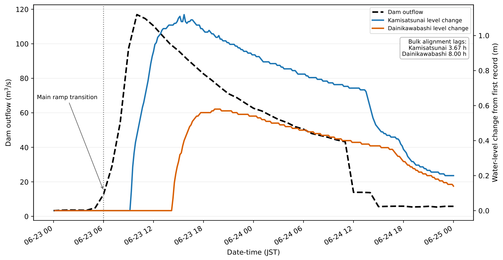
Within the project records available for this study, the 2026 event was the only period with concurrent and complete dam-outflow and water-level records at both far-field stations. It was therefore designated as the principal event. The analysis windows were defined from data availability and the documented release period before examining correlation results. The principal dam record covers 23–25 June 2026; outflow increased markedly during the morning of 23 June and reached 116.92 m³/s at 10:00 JST. 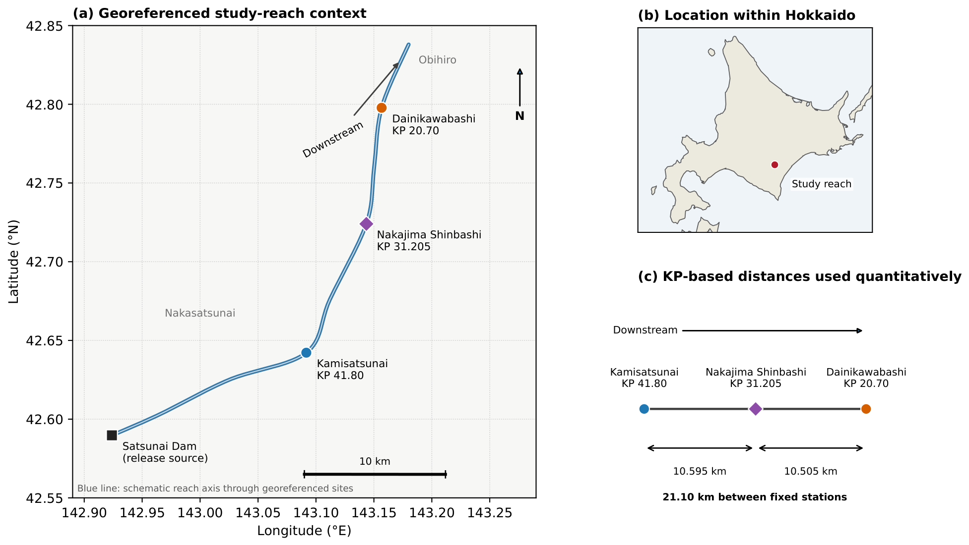Figure 1 shows Satsunai River Dam, Kamisatsunai, Dainikawabashi, and the intermediate Nakajima Shinbashi reference location. Official coordinates for the dam and fixed stations were taken from the MLIT station-information pages [19,20,21]. The intermediate reference coordinate and the kilometer-post values used quantitatively (KP 41.80, 31.205, and 20.70) were taken from project survey records; all reach distances and interpolation fractions were computed from those KP values.

Kamisatsunai is located at KP 41.80 and Dainikawabashi at KP 20.70, giving a documented station separation of 21.10 km. The water-level series cover 23 June 2026 00:10 to 30 June 2026 17:30 at 10-min resolution. Data completeness was checked before analysis. In the principal dam window (23 June 00:00–25 June 00:00), all 49 expected hourly outflow records were available. Each principal station window contained all 288 expected 10-min stage samples, and each full station record contained all 1113 expected samples; the missing fraction in these analyzed windows was therefore 0%.

A separate 2024 temporary-gauge dataset is presented as ancillary field context in the Supplementary Materials. Those records began after the release hydrograph had already increased, and the approximately 100 m gauge spacing is below the effective temporal resolution needed for a far-field propagation estimate. The 2024 data are therefore not used as validation of the 2026 result or as evidence of event-to-event invariance.

3.2. Time-Base Harmonization and Analysis Windows

Entries reported as 24:00 in the dam record were normalized to 00:00 of the following calendar day. The dam outflow was recorded hourly, whereas the stage was recorded every 10 min. A linear interpolation of the outflow was used only to evaluate the two signals on a common lag-search grid; it was not intended to reconstruct unresolved sub-hourly discharge dynamics. Zero-order-hold and native-hourly representations were also evaluated as input-representation sensitivity checks. The native-hourly calculation used only the 49 observed hourly dam values while sampling stage at candidate shifted times. The primary dam-to-station lag search covered 0–12 h. The direct station-to-station search covered $-8$ to $+8$ h.

Table 1. Principal 2026 analysis windows.

Signal Pair	Analysis Window	Purpose
Dam outflow vs. each far-field station	23 June 2026 00:00–25 June 2026 00:00	Dam-referenced bulk-lag estimation
Kamisatsunai vs. Dainikawabashi	23 June 2026 00:10–30 June 2026 17:30	Full-record direct comparison
Kamisatsunai vs. Dainikawabashi	23 June 2026 00:10–25 June 2026 00:00	Release-window direct comparison

summarizes the 2026 windows.

3.3. Cross-Correlation Lag and Peak Identifiability

For each station, the Pearson correlation coefficient was evaluated between the dam outflow $Q\left(t\right)$ and the lagged water level $H(t+\tau )$:

$$r\left(\tau \right)=\mathrm{corr}\left\{Q\right(t),H(t+\tau \left)\right\},\tau =0,10,20,\dots \min .$$

(1)

The grid maximum is

$$\widehat{\tau }=\arg \underset{\tau }{\max }r\left(\tau \right).$$

(2)

This quantity is a bulk hydrograph-alignment lag rather than a first-detectable-arrival time. Decimal-hour values identify 10-minute grid points and do not imply finer observational precision.

The maximizing grid point does not show how flat the correlation peak is. Peak identifiability was therefore also summarized using the descriptive near-optimal lag set

$${\mathcal{T}}_{0.995}=\{\tau :r\left(\tau \right)\ge 0.995r_{\max }\}.$$

(3)

This set is an identifiability diagnostic, not a confidence interval. Sensitivity to relative thresholds of 0.999 and 0.990 is reported in Supplementary Table S9.

3.4. Residual Dependence and Moving-Block Bootstrap

At each dam-to-station maximum, a linear relation, $H\left(t\right)\approx aQ(t-\widehat{\tau })+b$, was fitted over the valid overlap window, and the residual sequence was retained. Residual autocorrelation was examined to assess temporal dependence. Dependence remained substantial beyond 2 h, so moving-block sensitivity was evaluated using block lengths of 1, 2, 3, 4, 6, 8, 10, 12, 16, 20, and 24 h. For the two far-field stations, identical block indices were used on the common upstream-forcing grid to preserve cross-station residual dependence in derived quantities.

For each block length, L, the 2.5th and 97.5th percentiles of the bootstrap lag distribution were computed. To avoid treating any single block choice as definitive, block-length sensitivity was summarized by the envelope

$$I_{\mathrm{env}}=\left[\underset{L}{\min }{q}_{0.025}\left(L\right),\underset{L}{\max }{q}_{0.975}\left(L\right)\right].$$

(4)

We refer to this quantity as a block-length sensitivity envelope of percentile intervals; no nominal coverage is assigned to the envelope itself. The same block-length set was used for direct station-to-station residual bootstrap calculations. Residual autocorrelation and block-specific intervals are reported in Supplementary Figure S3 and Tables S3, S7 and S8; direct station-to-station block sensitivity is reported in Table S10. A fixed base random seed of 20260709 was used for the field bootstrap analyses.

3.5. Trend, Differencing, and Input-Representation Diagnostics

To test whether the high raw correlations were driven mainly by smooth shared trends, the dam-to-station lag search was repeated after separate linear detrending, unsmoothed first differencing, 1 h smoothing followed by differencing, and subtraction of a centered 6 h moving mean. The direct station-to-station analysis was repeated using the same classes of transformations for both the full record and the release window. Additional response definitions included persistent 10% rise crossing, a maximum 1 h rise, and peak-to-peak timing. These diagnostics measure feature and processing sensitivity and are not pooled into the bootstrap percentile intervals.

Hourly-input sensitivity was assessed using linear-interpolation, zero-order-hold, and native-hourly representations. Alignment-window sensitivity was evaluated using fixed upstream and fixed response windows. Full settings are provided in the Supplementary Materials.

3.6. Internal Temporal Closure, Apparent Celerity, and Spatial Interpolation

The far-field records provide two calculation paths to a reach-scale timing difference. The first is the difference between dam-referenced lags, ${\widehat{\tau }}_D-{\widehat{\tau }}_K$. The second is the direct water-level alignment lag ${\widehat{\tau }}_{K\to D}$. Their agreement is summarized by

$${\delta }_c=({\widehat{\tau }}_D-{\widehat{\tau }}_K)-{\widehat{\tau }}_{K\to D}.$$

(5)

A small closure residual indicates agreement between the two calculations. Because the same downstream records enter both paths, the comparison is an internal check rather than statistically independent validation.

Apparent celerity was calculated as

$$c={\displaystyle \frac{\Delta d}{{\widehat{\tau }}_D-{\widehat{\tau }}_K}},$$

(6)

where $\Delta d=21.10$ km. Here, ${\widehat{\tau }}_D$ and ${\widehat{\tau }}_K$ denote the dam-referenced alignment lags at Dainikawabashi and Kamisatsunai, respectively. It is interpreted as a reach-averaged timing descriptor rather than local velocity or locally defined kinematic-wave celerity.

Nakajima Shinbashi at KP 31.205 lies between the two fixed stations. Its event-specific lag was estimated by linear interpolation,

$${\widehat{\tau }}_R={\widehat{\tau }}_K+{\displaystyle \frac{41.80-31.205}{41.80-20.70}}({\widehat{\tau }}_D-{\widehat{\tau }}_K).$$

(7)

The same expression was applied to paired bootstrap replicates. This produces a conditional sampling estimate under a constant reach-averaged timing-fraction assumption. It does not incorporate hydraulic spatial model-form uncertainty. A separate structural stress test perturbed the normalized timing fraction by $\pm 10\%$ and $\pm 20\%$ relative to the distance fraction; those scenarios are reported separately in Supplementary Table S15 and are not treated as probability bounds.

3.7. Synthetic Implementation Check

The implementation was also tested on synthetic responses with known lags. The standardized observed release shape was used as the driver. Synthetic responses were shifted by 3.67 and 8.00 h, and AR(1) residual noise was added. Two persistence settings ($\varphi =0.65$ and 0.95; noise scale 0.12) were evaluated over 1000 replicates per station and setting. This exercise checks lag recovery under controlled conditions; it does not test hydraulic transferability. The results are reported in Supplementary Figure S4 and Table S14. All analyses were conducted in Python 3.13.5 using pandas 2.2.3, NumPy 2.3.5, openpyxl 3.1.5, Matplotlib 3.10.8, pyproj 3.7.2, and Basemap 2.0.0.

4. Results

4.1. 2026 Release and Far-Field Response

Figure 2 shows the 2026 release and far-field responses. The release transitioned into the main ramp around 06:00 JST on 23 June, followed by delayed water-level changes at Kamisatsunai and Dainikawabashi. The annotations show the bulk alignment lags and are not first-arrival markers.

4.2. Dam-Referenced Lags and Correlation-Peak Width

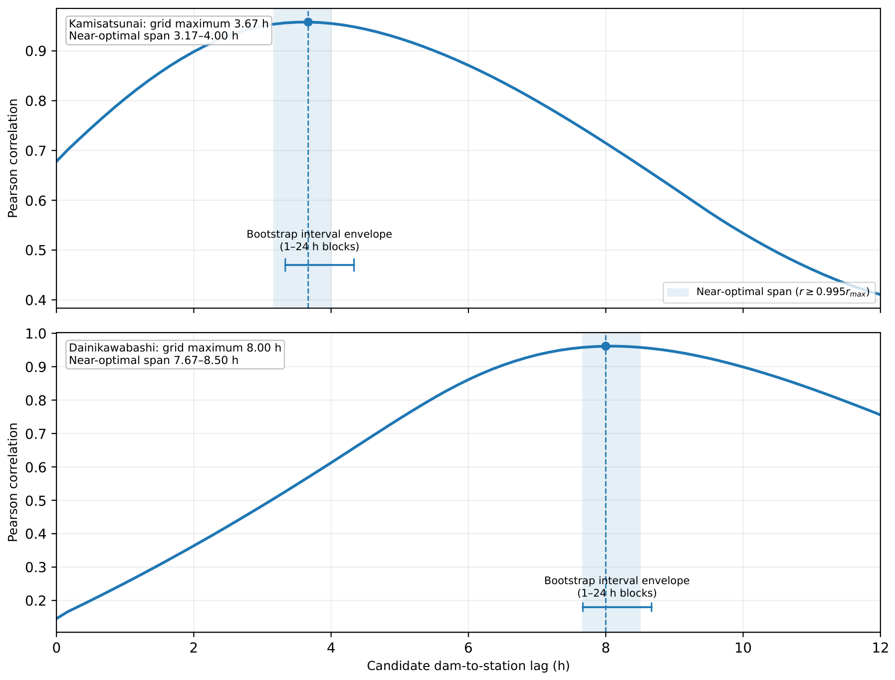
The raw grid maxima were 3.67 h at Kamisatsunai and 8.00 h at Dainikawabashi.

Table 2. Dam-referenced bulk alignment results for the 2026 far-field stations. The near-optimal span is descriptive; the bootstrap column is the envelope of 2.5th–97.5th percentile intervals over 1–24 h block lengths.

Station	KP	Grid Maximum (h)	${\mathit{r}}_{\max }$	Near-Optimal Span (h)	Bootstrap Interval Envelope (h)
Kamisatsunai	41.80	3.67	0.958	3.17–4.00	3.33–4.33
Dainikawabashi	20.70	8.00	0.961	7.67–8.50	7.67–8.67

distinguishes the grid maximum, a descriptive near-optimal span, and the block-length sensitivity envelope of bootstrap percentile intervals.

At Kamisatsunai, the 99.5%-of-maximum span covered 3.17–4.00 h; at Dainikawabashi it covered 7.67–8.50 h. Threshold sensitivity confirms that these widths increase as the criterion is relaxed (Supplementary Table S9). Figure 3 displays the objective-function flatness separately from the bootstrap sensitivity envelope.

4.3. Robustness to Smooth Trend and Signal Transformation

The dam-to-station transformation analysis is summarized in

Table 3. Dam-to-station lag sensitivity to trend removal and differencing.

Transformation	Kamisatsunai Lag (h)	Dainikawabashi Lag (h)	Separation (h)	${\mathit{r}}_{\mathit{K}}$	${\mathit{r}}_{\mathit{D}}$
Raw levels	3.67	8.00	4.33	0.958	0.961
Separate linear detrending	3.17	7.17	4.00	0.977	0.962
First differences	2.50	6.17	3.67	0.674	0.647
1 h smoothed differences	2.67	6.67	4.00	0.853	0.830
6 h moving-mean detrending	2.33	6.67	4.33	0.836	0.834

. The individual endpoint maxima changed because different transformations emphasize different hydrograph features. More importantly for the reach-scale comparison, station ordering was unchanged, and the separation between the two endpoint lags remained 3.67–4.33 h. Thus, the multi-hour separation was not produced solely by the shared smooth hydrograph shape.

Direct station-to-station transformations gave 4.00–5.00 h over the release window and 4.33–5.00 h over the full record, consistent with a multi-hour reach-scale response rather than a unique physical arrival instant. Detailed direct results and alternative response definitions are provided in Supplementary Tables S2 and S6.

4.4. Internal Temporal Closure and Block-Length Sensitivity

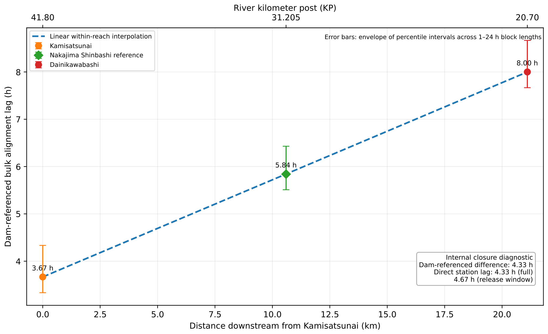
The raw dam-referenced lag difference was 4.33 h. Direct station-to-station alignment gave 4.33 h over the full record and 4.67 h over the release window, producing closure residuals of 0.00 and $-0.33$ h, respectively (

Table 4. Internal temporal-closure diagnostic for the 2026 far-field reach.

Estimate Path	Reach-Scale Time (h)	Closure Residual (h)
Difference of raw dam-referenced maxima	4.33	Reference
Direct station-to-station, full record	4.33	0.00
Direct station-to-station, release window	4.67	$-0.33$

). The two calculations agree within 0.33 h. Because they share the same downstream records, this agreement is an internal temporal-closure check rather than independent validation.

Residual ACFs showed material dependence beyond 2 h, motivating the expanded block analysis rather than a single preferred block. Across 1–24 h blocks, the envelope of paired far-field percentile intervals was 4.17–4.50 h for the lag difference and 1.30–1.41 m/s for apparent celerity. Direct full-record percentile intervals formed an envelope of approximately 3.67–4.67 h, while the release-window envelope was 4.50–4.83 h. Point estimates were unchanged. Block-specific endpoint results are reported in Supplementary Tables S3 and S8, and the direct station-to-station block analysis is reported in Table S10.

4.5. Hourly-Input Representation

Zero-order hold gave lags of 3.17 h (Kamisatsunai) and 7.67 h (Dainikawabashi). The native-hourly calculation, using only the observed hourly dam values, gave 3.67 and 8.33 h. These checks shift individual endpoint maxima by several 10-minute grid steps but retain the station ordering from upstream to downstream and the multi-hour separation. The 10-minute linear interpolation is therefore treated as a time-base convention rather than evidence of sub-hourly discharge dynamics.

4.6. Intermediate-Location Estimate and Uncertainty Separation

The raw 4.33 h lag difference over 21.10 km corresponds to an apparent celerity of approximately 1.35 m/s, while the 4.67 h direct release-window timing corresponds to approximately 1.26 m/s. The block-length envelope based on the paired dam-referenced difference is 1.30–1.41 m/s.

Linear interpolation places the Nakajima Shinbashi reference estimate at 5.84 h. Across 1–24 h paired block settings, the envelope of the conditional percentile intervals was 5.51–6.43 h (Figure 4). This interval describes residual resampling and block-length sensitivity under the linear spatial interpolation assumption. It does not include uncertainty from nonuniform within-reach hydraulics. In the separate structural stress test, changing the normalized timing fraction by $\pm 10\%$ from the distance fraction shifted the estimate by $\pm 0.22$ h, and a $\pm 20\%$ change shifted it by $\pm 0.44$ h. These are illustrative scenarios, not confidence limits.

4.7. Synthetic Known-Lag Implementation Check

The synthetic test recovered the imposed median lags at both 3.67 and 8.00 h under both persistence settings. Recovery was concentrated near the imposed lags at moderate persistence and broadened under stronger serial persistence; detailed recovery frequencies and ranges are reported in Supplementary Figure S4 and Table S14.

4.8. Uncertainty Inventory

Table 5. Uncertainty and sensitivity sources in this analysis.

Source	Treatment in this Study	Status
Residual sampling variability and serial dependence	Moving-block bootstrap sensitivity spanning 1–24 h; percentile-interval envelope	Conditional quantification
Correlation-peak flatness	$r\ge 0.995r_{\max }$ near-optimal span; threshold sensitivity at 0.999 and 0.990	Descriptive quantification
Low-frequency trend/signal feature	Linear detrending, first differences, smoothed differences, moving-mean detrending	Sensitivity test
Timing definition	Whole level, rising-limb, detrended, maximum-rise, and peak timing diagnostics	Sensitivity test
Hourly dam-input representation	Linear interpolation, zero-order hold, and native-hourly calculation	Sensitivity test
Analysis-window convention	Fixed upstream and fixed response windows	Sensitivity test
Within-reach spatial model form	Linear interpolation plus normalized timing-fraction stress scenarios	Scenario test; not probabilistic
Unmonitored lateral/tributary inflows, channel geometry, storage, and backwater	No event-specific measurements sufficient for separation	Qualitative; unquantified
Event-to-event variability	One principal fully observed event	Unquantified

distinguishes quantities that are directly quantified, sensitivity-tested, or only bounded qualitatively with the available observations.

5. Discussion

5.1. Internal Closure and Uncertainty Separation

The agreement between the dam-referenced lag difference and the direct station-to-station estimate provides an internal consistency check for the 2026 event: the former is 4.33 h, while the direct estimates are 4.33 h for the full record and 4.67 h for the release window. The analysis also keeps several sources of uncertainty separate rather than combining them into a single interval. These include peak flatness, trend sensitivity, hourly-input representation, timing definition, residual dependence, spatial model form, and event-to-event variability. The intermediate-location estimate is then reported conditionally on the stated spatial-interpolation assumption.

The direct and dam-referenced calculations are computationally distinct but statistically dependent because they share the two downstream records. Their agreement is therefore an internal closure diagnostic, not external validation.

5.2. Autocorrelation, Peak Flatness, and Timing Identifiability

The raw maximum correlations near 0.96 are influenced by the smooth, autocorrelated character of the forcing and response series. The transformation results show why correlation magnitude alone is not the main evidence. Differencing reduced the peak correlations substantially, yet the endpoint separation remained 3.67–4.33 h and the direct transformed station-to-station results remained in a 4–5 h range. The near-optimal spans also show that neighboring lags align the records almost equally well. Taken together, these checks support a consistent multi-hour event-scale timing structure, but not a uniquely identified physical arrival instant.

Residual dependence also affects the bootstrap results. The ACF analysis did not identify 2 h as a uniquely preferred block length, so the 1–24 h results are summarized as an envelope. The lag-difference and celerity intervals were comparatively stable across this range, whereas the endpoint and intermediate-location upper bounds showed somewhat greater block sensitivity.

5.3. Relation to Hydraulic Routing

The present analysis is intended for an information-limited setting and complements calibrated hydraulic routing when the inputs required for calibration are unavailable. A calibrated Muskingum comparison normally requires reach inflow and outflow hydrographs for parameter identification or an independently supported parameter set [7]. Here, the far-field observations are water level rather than downstream discharge, and event-specific rating curves, lateral inflows, and calibration events were unavailable. A Saint-Venant-type comparison would also require consistent geometry, roughness, and boundary information. Hydraulic-model calibration can itself exhibit substantial parameter uncertainty and equifinality when roughness and boundary information are weakly constrained [22]. Using assumed parameters would therefore introduce model uncertainty that could not be assessed with these data, so such a calculation was not used as an independent benchmark.

Where the required inputs are available, calibrated routing supports physically based prediction. The present analysis instead targets event-specific timing from sparse stage records and can support interpretation and scheduling of downstream observations. Operational forecasting would require additional hydraulic information and multi-event evaluation.

5.4. Comparison with Published River Studies and Local Satsunai Context

The apparent celerity of 1.26–1.35 m/s inferred from the two point definitions, and the 1.30–1.41 m/s block-sensitivity envelope, fall within the broad range reported for flood-wave celerity in previous river studies. Meyer et al. [14] reported values spanning approximately 0.2–7.5 m/s across 12 Brazilian river reaches, with reach-scale averages near 1.78 m/s, while emphasizing strong dependence on discharge, river geometry, and estimation method. Because the rivers, events, and timing definitions differ, the comparison is only a scale reference.

The local Satsunai studies also show why direct numerical comparisons need to be treated cautiously. Yanagiya et al. [8] evaluated artificial flash releases with field discharge measurements and one- and two-dimensional calculations. Tsubaki and Zhu [9] studied a 2020 flushing release with a peak of approximately 110 m³/s and reported a representative local surface velocity of 2.39 m/s at their image-observation site. That velocity is a different physical quantity from the reach-averaged bulk alignment celerity reported here. Takahashi and Nakamura [10] showed that tributary inflows can mitigate dam-regulated effects in lower Satsunai reaches, supporting the present treatment of unmonitored lateral inflow as structural uncertainty rather than a negligible term.

5.5. Spatial Interpolation and Transfer Limits

The 5.84 h value at Nakajima Shinbashi is a linear-interpolation estimate within the observed station pair. Its 5.51–6.43 h block-sensitivity envelope is conditional on that interpolation form. The structural timing-fraction scenarios show that modest nonlinearity can shift the point estimate by several tenths of an hour, comparable to the conditional sampling width. The interpolation therefore provides a planning reference for this event, not a locally resolved hydraulic prediction.

The numerical lags are not expected to transfer directly to another release, discharge regime, or river. The analysis sequence itself can be reapplied: endpoint lag estimation, peak-width assessment, transformed-signal robustness checks, internal closure, serial-dependence sensitivity, and separation of spatial model-form uncertainty. Its behavior across events can only be assessed with additional controlled releases and synchronized observations.

5.6. Ancillary 2024 Observations

The 2024 temporary-gauge records are presented only in the Supplementary Materials. Their late start and approximately 100 m spacing do not support an equivalent far-field validation analysis. They are therefore used as ancillary context rather than as replication of the 2026 event.

6. Limitations

This study is based on one controlled release on one river, observed at two far-field stations, so its numerical lags cannot yet be generalized to natural floods, other discharge ranges, or other regulated rivers. The closure comparison is also internal because both calculation paths use the same downstream records.Cross-correlation measures bulk hydrograph alignment rather than first arrival, and the individual lag estimates depend on the signal feature emphasized; the broad correlation peaks further limit temporal resolution. The moving-block results remain conditional on the residual model.

The intermediate-location estimate has a separate limitation: only two endpoint stations constrain the spatial timing pattern. Tributary inflows and the geometry, storage, roughness, and backwater information needed for a calibrated hydraulic comparison were not available. Additional releases, denser monitoring, discharge/rating information, tributary observations, and hydraulic surveys are therefore needed before operational or cross-event use.

7. Conclusions

For the principal 2026 Satsunai River controlled release, the dam-referenced bulk alignment maxima were 3.67 h at Kamisatsunai and 8.00 h at Dainikawabashi. Their 4.33 h separation matched the full-record direct station-to-station maximum and was close to the 4.67 h release-window result. Detrending and differencing changed the individual endpoint maxima, but the separation remained 3.67–4.33 h, indicating a multi-hour reach-scale timing pattern beyond the shared smooth trend.

The correlation peaks were broad enough to limit temporal precision: the near-optimal spans were 3.17–4.00 h and 7.67–8.50 h. Residual autocorrelation did not support relying on a single 2 h bootstrap block, so sensitivity was examined over 1–24 h. The paired lag-difference percentile envelope was 4.17–4.50 h, corresponding to an apparent celerity of 1.30–1.41 m/s.

Under linear within-reach interpolation, the estimate at Nakajima Shinbashi was 5.84 h, with a conditional percentile-interval envelope of 5.51–6.43 h. This range does not include uncertainty in the spatial hydraulic model form. Taken together, the results provide a consistent event-specific description of downstream bulk response timing from the available sparse records. Additional synchronized events and hydraulic observations are needed to evaluate transferability and predictive routing applications.

References

- Shook, K.R.; Whitfield, P.H.; Spence, C.; Pomeroy, J.W. Estimating Response Times, Flow Velocities, and Roughness Coefficients of Canadian Prairie Basins. Hydrol. Earth Syst. Sci. 2024, 28, 5173–5192. [Google Scholar] [CrossRef] [Scilit]
- Archer, D.R.; Fileni, F.; Watkiss, S.A.; Fowler, H.J. Characteristics of Gauged Abrupt Wave Fronts (Walls of Water) in Flash Floods in Scotland. Hydrol. Earth Syst. Sci. 2025, 29, 5777–5789. [Google Scholar] [CrossRef] [Scilit]
- Carter, R.W.; Godfrey, R.G. Storage and Flood Routing; U.S. Geological Survey Water-Supply Paper 1543-B; U.S. Government Printing Office: Washington, DC, USA, 1960.
- Chow, V.T. Open-Channel Hydraulics; McGraw-Hill: New York, NY, USA, 1959. [Google Scholar]
- Fread, D.L. Channel Routing. In Hydrological Forecasting; Anderson, M.G., Burt, T.P., Eds.; Wiley: Chichester, UK, 1985; pp. 437–503. [Google Scholar]
- Cunge, J.A. On the Subject of a Flood Propagation Computation Method (Muskingum Method). J. Hydraul. Res. 1969, 7, 205–230. [Google Scholar] [CrossRef] [Scilit]
- Wang, W.-C.; Tian, W.-C.; Xu, D.-M.; Chau, K.-W.; Ma, Q.; Liu, C.-J. Muskingum Models’ Development and Their Parameter Estimation: A State-of-the-Art Review. Water Resour. Manag. 2023, 37, 3129–3150. [Google Scholar] [CrossRef] [Scilit]
- Yanagiya, K.; Izumi, N.; Kakinuma, T.; Takeda, A. Experimental Flow Release by a Dam for Reproducing Gravel Bed in Satsunai River. Adv. River Eng. 2014, 20, 319–324. [Google Scholar] [CrossRef] [PubMed]
- Tsubaki, R.; Zhu, R. Optical Ortho-Rectification for Image-Based Stream Surface Flow Observations Using a Ground Camera. Front. Water 2021, 3, 700946. [Google Scholar] [CrossRef] [Scilit]
- Takahashi, M.; Nakamura, F. Impacts of Dam-Regulated Flows on Channel Morphology and Riparian Vegetation: A Longitudinal Analysis of Satsunai River, Japan. Landsc. Ecol. Eng. 2011, 7, 65–77. [Google Scholar] [CrossRef] [Scilit]
- World Meteorological Organization. Manual on Stream Gauging; WMO-No. 1044; World Meteorological Organization: Geneva, Switzerland, 2010. [Google Scholar]
- Sales, L.O.; Lappicy, T.; Beltrão, D.; de Amorim Teixeira, A.; Cicerelli, R.; Almeida, T. SWOT Satellite Nodes as Virtual Stations During the 2024 Extreme Flood in Southern Brazil. Hydrology 2025, 12, 248. [Google Scholar] [CrossRef] [Scilit]
- Tauro, F.; Selker, J.; van de Giesen, N.; Abrate, T.; Uijlenhoet, R.; Porfiri, M.; Manfreda, S.; Caylor, K.; Moramarco, T.; Benveniste, J.; et al. Measurements and Observations in the XXI Century (MOXXI): Innovation and Multi-Disciplinarity to Sense the Hydrological Cycle. Hydrol. Sci. J. 2018, 63, 169–196. [Google Scholar] [CrossRef] [Scilit]
- Meyer, A.; Fleischmann, A.S.; Collischonn, W.; Paiva, R.; Jardim, P. Empirical Assessment of Flood Wave Celerity–Discharge Relationships at Local and Reach Scales. Hydrol. Sci. J. 2018, 63, 2035–2047. [Google Scholar] [CrossRef] [Scilit]
- Kilpatrick, F.A.; Wilson, J.F. Measurement of Time of Travel in Streams by Dye Tracing; U.S. Geological Survey Techniques of Water-Resources Investigations, Book 3, Chapter A9; U.S. Geological Survey: Reston, VA, USA, 1989. [CrossRef] [Scilit]
- Jobson, H.E. Estimating the Variation of Travel Time in Rivers by Use of Wave Speed and Hydraulic Characteristics; U.S. Geological Survey Water-Resources Investigations Report 2000-4187; U.S. Geological Survey: Reston, VA, USA, 2000. [CrossRef] [Scilit]
- Künsch, H.R. The Jackknife and the Bootstrap for General Stationary Observations. Ann. Stat. 1989, 17, 1217–1241. [Google Scholar] [CrossRef] [Scilit]
- Beven, K.; Binley, A. The Future of Distributed Models: Model Calibration and Uncertainty Prediction. Hydrol. Processes 1992, 6, 279–298. [Google Scholar] [CrossRef] [Scilit]
- Ministry of Land, Infrastructure, Transport and Tourism. Hydrological and Water Quality Database: Satsunai River Dam Station Information. Available online: https://www1.river.go.jp/cgi/SiteInfo.exe?ID=1368010829410 (accessed on 19 July 2026).
- Ministry of Land, Infrastructure, Transport and Tourism. Hydrological and Water Quality Database: Kamisatsunai Station Information. Available online: https://www1.river.go.jp/cgi/SiteInfo.exe?ID=301081281107210 (accessed on 19 July 2026).
- Ministry of Land, Infrastructure, Transport and Tourism. Hydrological and Water Quality Database: Dainikawabashi Station Information. Available online: https://www1.river.go.jp/cgi/SiteInfo.exe?ID=301081281107220 (accessed on 19 July 2026).
- Pappenberger, F.; Beven, K.; Horritt, M.; Blazkova, S. Uncertainty in the Calibration of Effective Roughness Parameters in HEC-RAS Using Inundation and Downstream Level Observations. J. Hydrol. 2005, 302, 46–69. [Google Scholar] [CrossRef] [Scilit]