


Abstract
Accurate calibration of Manning’s roughness coefficients is essential for reliable river hydraulic modelling, flood prediction, and water resources management, yet conventional calibration methods often struggle with high-dimensional parameter spaces and nonlinear hydraulic interactions. This study proposes and evaluates a hierarchical artificial intelligence framework for the inverse calibration of spatially distributed Manning’s roughness coefficients across three channel zones (left bank, main channel, and right bank), using a 48 km reach of the Tigris River in Baghdad as a case study. A one-dimensional HEC-RAS hydraulic model based on 30 measured cross-sections generated 18,360 simulations by systematically varying Manning’s roughness coefficients (0.02–0.045). Three calibration strategies were evaluated: (i) a simple Gradient Boosting Regression model based on a weighted composite roughness formula, (ii) conventional machine learning models (Random Forest, Gradient Boosting, and Multi-Layer Perceptron), and (iii) a deep learning framework combining a three-layer neural network (64 → 32 → 16 neurons), Differential Evolution optimisation, and cubic spline interpolation. Calibration accuracy increased with model complexity. The deep learning framework achieved the best performance, reducing the root mean square error by 96.6% (from 1.202 to 0.041 m), with R2 = 0.992 and negligible bias (−0.004 m). Conventional machine learning models produced spatially variable Manning’s roughness distributions, with the calibrated main-channel roughness (mean n = 0.0512) being 34.0–57.5% higher than the corresponding bank values. The proposed framework provides an effective approach for calibrating spatially distributed roughness coefficients in one-dimensional hydraulic models, with strong potential to improve river hydraulic simulations and support future applications to flood modelling.
1. Introduction
River hydraulic models are essential tools for predicting water flow, flood risk, and water management decisions, but the quality of these predictions is sensitive to the appropriate calibration of model parameters [1]. Conventional calibration procedures use manual parameter optimization or optimization algorithms, which are time-consuming and may fail to capture complex parameter-model output interactions. Such traditional methods tend to fail to address the high-dimensional spaces of parameters and non-linear relationships that are characteristic of hydraulic systems and thus provide suboptimal results in calibration [2].
One of the most relevant parameters in river hydraulic modelling is Manning’s roughness coefficient since it is a direct determinant of the calculation of flow velocity in the Manning equation and other equations of the flow resistance [3,4,5]. Conventional ways of calculating the Manning’s roughness coefficient are based on measurements in the field, a lookup table depending on the nature of the channel, or manual methods to calculate this coefficient by trial and error, which is time-consuming and may produce uncertain outcomes [6]. The coefficient is highly sensitive to other factors such as the bed material, vegetation, channel geometry, and seasonal variations, and estimating it accurately may be difficult in other river reaches and flow regimes [7,8].
HEC-RAS has emerged as a particularly prominent open-access computational modelling tool in flood modelling because of its versatility, free availability, and applicability to one-dimensional and two-dimensional hydraulic analyses [9]. The model is regularly employed for the calibration and validation of water surface profiles in a wide range of channel configurations, including compound channels with complex geometries [10,11]. Its widespread adoption has also encouraged the integration of machine learning techniques with HEC-RAS to improve flood modelling and prediction capabilities [12,13,14,15,16]. Using spatiotemporal data with daily rainfall, temperature, and topographical wetness indices, they are first trained to predict runoff with artificial neural networks, and then the output of the ANN is processed by HEC-RAS software Version 5.0.6 to produce flood extent on rivers [17]. This combined system identified the flood-prone areas with a machine learning integration with HEC-RAS with nearly 96% accuracy compared to the delineation of water bodies using satellite images, which shows that integrating machine learning with HEC-RAS has enhanced the spatiotemporal uncertainties in the conventional methods of flood forecasting [18].
Random Forest has been especially useful in hydraulic model calibration because it is capable of dealing with nonlinear relationships of interest and is resistant to overfitting. Random Forest classification models in flood prediction have recorded high accuracy levels of over 98% when applied to detect wet and dry nodes in river areas [19]. Its usefulness is also applicable to hydrologic exchange flow modeling, where the Random Forest and Extreme Gradient Boosting models can be used with 70% to 80% accuracy as substitutes for computationally intensive numerical models [20,21,22,23,24,25]. Random Forest algorithms can also be combined with HEC-RAS, in which machine learning-generated discharge values are used as input parameters to hydraulic modeling [26,27]. The method enables the combination of models operating on hydrological and hydraulic scales, which have become increasingly popular in flood risk management [28,29,30].
Extreme Gradient Boosting (XGBoost) has become a better substitute for the conventional approaches to streamflow forecasting and hydraulic modeling [31]. XGBoost combines the merits of gradient boosting and decision tree algorithms and shows better performance in comparison with Random Forest and Classification and Regression Trees (CART) models—the relative errors of XGBoost are 2.18–9.21% versus 3.76–10.41% [32]. The scalability and efficiency of the method have been especially useful in large-scale applications [33]. Deep learning surrogate models represent a major development in computational efficiency in flood modeling applications [34,35,36]. Researchers have been able to train various deep learning models, such as MLP, RNN, CNN, LSTM, and RCNN, to be used as surrogate models to quickly predict water stage, and with the far-reaching extensiveness of experiments, they have discovered that such DL models can noticeably improve over the physics-based HEC-RAS model, even in extreme precipitation conditions such as tropical storms, and with speedups by over 500×. This responds to the dire requirement of surrogate models to quickly and precisely forecast water surface elevations on the river at a certain point [37,38].
Despite the substantial progress achieved in applying artificial intelligence to hydraulic modelling, most existing studies have focused on flood prediction, surrogate modelling, computational acceleration, or related hydraulic applications, including recent approaches based on HEC-RAS-generated datasets for extreme-event forecasting [39,40,41,42,43,44,45]. Although these studies have demonstrated the potential of AI to improve predictive capability and computational efficiency, comparatively little attention has been given to the inverse calibration of spatially distributed Manning’s roughness coefficients within established hydraulic models. In particular, the estimation of physically meaningful roughness distributions in complex river systems remains challenging because of the large number of calibration parameters, the nonlinear interactions among hydraulic variables, and the possibility that different parameter combinations produce similar hydraulic responses. Consequently, conventional calibration methods, whether based on manual trial-and-error or optimization algorithms, often rely on simplified assumptions, such as uniform roughness values, that cannot adequately represent the spatial variability of natural river channels. Table 1 summarizes the main differences between the present study and previously published AI-based approaches for hydraulic model calibration.
Table 1.
Comparison of the present study with previous AI-based calibration approaches for hydraulic models.
To address these challenges, this study develops and comparatively evaluates a hierarchical artificial intelligence-based calibration framework for estimating spatially distributed Manning’s roughness coefficients in a 48 km reach of the Tigris River in Baghdad. Three levels of increasing model complexity are investigated, namely a simple Gradient Boosting-based approach, conventional machine learning models (Random Forest, Gradient Boosting, and Multi-Layer Perceptron), and a deep learning architecture. The proposed framework is assessed in terms of its ability to improve the calibration accuracy of a one-dimensional HEC-RAS model while representing the spatial variability of Manning’s roughness coefficients across the left bank, main channel, and right bank. The main contribution of this work is the systematic comparison of progressively more sophisticated AI-based calibration strategies for the inverse estimation of spatially distributed roughness coefficients within a hydraulic modelling framework.
The novelty of the present study does not reside in the individual AI or optimisation algorithms, which are established methods, but in their integration and systematic comparison within an inverse-calibration framework specifically designed to estimate spatially distributed Manning’s roughness coefficients. In contrast to the predominantly forward-prediction and surrogate-modelling applications summarised in Table 1, the present framework estimates roughness across three hydraulic zones (left bank, main channel, and right bank) at 30 stations along the investigated river reach. Furthermore, the hierarchical comparison of progressively more sophisticated calibration strategies provides a consistent basis for assessing how increasing model complexity affects calibration performance within the same hydraulic case study. This combination of spatially distributed inverse calibration and hierarchical comparative evaluation constitutes the principal methodological contribution of the present study.
2. Materials and Methods
2.1. Methodology
The methodology adopted in this study consists of a hierarchical AI-based calibration framework designed to estimate spatially distributed Manning’s roughness coefficients within a 48 km stretch of the Tigris River in Baghdad (Figure 1). To start with, a one-dimensional steady-flow hydraulic model was created with the help of HEC-RAS, including 30 surveyed cross-sections, which were divided into three separate areas: left bank, main channel, and right bank. These zones were systematically and carefully varied in Manning n values (0.02 to 0.045) to produce a comprehensive dataset of 18,360 hydraulic responses. It was based on this dataset that three levels of escalating AI-based calibration strategies were trained and evaluated: a basic model that used Gradient Boosting with Nelder–Mead optimization and a weighted composite roughness formula; more familiar machine learning models, which encompassed the Random Forest, Gradient Boosting, and a Multi-Layer Perceptron (MLP); and a state-of-the-art deep learning model that used a three-layer neural network architecture (64 → 32 → 16 neurons) and a global optimization method using differential evolution.
Figure 1.
Overview of the hierarchical AI-based calibration framework adopted in this study.
Minimization of the root mean square error (RMSE) between the calculated water surface elevations using HEC-RAS and measured field data at 30 stations with a 700 m3/s discharge was the driving force of the calibration process. In the case of the machine learning and deep learning models, the dataset was divided into 80% training and 20% test, and regularization methods, including dropout and early stopping, were used to avoid overfitting and improve generalization. The 80/20 data split employed during AI model training applies exclusively to the synthetic HEC-RAS simulation dataset and assesses surrogate generalization within that parameter space only. The deep learning model also included cubic spline interpolation to provide smooth and physically continuous changes in roughness coefficients between stations so that it could best represent local changes in roughness as well as global hydraulic gradients. This approach made it possible to compare the capability of each of the methods to study the high-dimensional, nonlinear parameter space and to generate physically plausible, spatially varying roughness estimates throughout the three channel regions. The developed models are valid only near a discharge of 700 m3/s; extrapolation to largely different discharge regimes or flood conditions is beyond the scope of this study.
The overall methodology consisted of three main stages. First, a one-dimensional HEC-RAS model was developed and used to generate a large database of hydraulic simulations by systematically varying Manning’s roughness coefficients. Second, this database was used to train three hierarchical AI-based calibration strategies of increasing complexity. Finally, the calibrated models were evaluated and compared using hydraulic performance indicators and validation analyses.
2.2. Study Reach and Data Collection
The study focuses on a crucial reach of the Tigris River inside Baghdad, Iraq, namely the 47,950 m (about 48 km) stretch between the Al Muthanna Bridge and the point where it joins the Diyala River. The extent is defined as a row of surveyed cross-sections of 30 different stations, identified numerically with designations from 950 down to 47,950, that characterize the morphological variability of the river [46]. The stations have elaborated geometric information, such as the river centerline, bank lines, and subdivision of each cross-section into three distinct areas: the left overbank, the main channel, and the right overbank. This space demarcation is essential in the determination of the roughness coefficients of distributed Manning because the resistance to the flow of the main channel bed may be very different compared to the vegetated or irregular banks of the floodplain. Figure 2 illustrates the location of the investigated reach of the Tigris River within Baghdad, together with the distribution of the surveyed cross-sections used for hydraulic model development and calibration.
Figure 2.
Location of the study reach along the Tigris River in Baghdad, Iraq, showing the surveyed cross-sections used to define the HEC-RAS river geometry.
The hydraulic model is based on detailed topographic and hydraulic data collected up and down this reach. The hydraulic data contain 204 cross-sections of the Tigris River, with water surface elevation in 30 cross-sections at a discharge of 700 m3/s (which was done previously by the General Authority of Survey, Ministry of Water Resources), Table 2. These data involved topographic measurements and the river direction and its geometry [47].
Table 2.
Locations for observing water surface elevation.
In total, 204 surveyed cross-sections were used to define the river geometry in the HEC-RAS model, whereas only the 30 cross-sections for which observed water-surface elevations were available at the 700 m3/s discharge were used for calibration against field data. Figure 2 therefore shows the larger set of geometric cross-sections, while Table 2 lists the 30 calibration stations.
2.3. Hydraulic Model Development
HEC-RAS software Version 5.0.6 is then used to prepare the one-dimensional steady-flow hydraulic model of the Tigris River reach. The river geometry was defined from the surveyed cross-sections, each of which was subdivided into three hydraulic regions (left overbank, main channel, and right overbank), as illustrated in Figure 3. The river geometry was defined from the surveyed cross-sections, each of which was subdivided into three hydraulic regions (left overbank, main channel, and right overbank), as illustrated in Figure 3. The boundaries between the main (minor) channel and the left and right overbanks at each cross-section were defined using the bank stations identified during the topographic survey of the study reach. These surveyed bank stations were subsequently used in the HEC-RAS geometric representation to delineate the three hydraulic regions. The sensitivity of the calibrated roughness distribution to alternative channel delineations was not investigated in the present study. However, a sensitivity analysis similar to that proposed for minor-riverbed delineation in small-hydropower applications [48] could be considered in future work to assess the robustness of the adopted channel subdivision. The hydraulic model was developed using the measured upstream discharge and the observed water surface elevations at the 30 surveyed cross-sections listed in Table 2.
Figure 3.
Representative cross-sections of the Tigris River reach illustrating the subdivision into the left overbank, main channel, and right overbank adopted for HEC-RAS model development and Manning’s roughness calibration.
The Manning equation in HEC-RAS is not merely used to predict flow velocity but is actually embedded into the heart of the software to calculate friction loss and conveyance, which are critical in calculating the water surface profiles. In each cross-section, HEC-RAS first splits the flow areas according to variations in the Manning’s roughness coefficient to determine the conveyance (K), a check of the carrying capacity of the discharge of that subsection, as
where k is a unit conversion factor (1.0 in the SI system and 1.486 in the Imperial system), A is the cross-sectional area of flow (R2), and R is the hydraulic radius (n).
The conveyances of the left overbank, main channel, and right overbank are then summed by the program to obtain the total conveyance for each cross-section. This total conveyance is subsequently applied to calculate the slope of the energy grade line (Sf) between sections, which is the slope of the energy grade line calculated as in the equation of Manning as
where Q is the discharge (m3/s). This friction slope is a very crucial element in the standard step procedure that HEC-RAS repeatedly provides to model water surface profiles of steady, gradually varied flow [49]. For the generation of the synthetic hydraulic dataset, Manning’s roughness coefficients were systematically varied within the range 0.020–0.045 for the left bank, main channel, and right bank, and the corresponding water surface elevations were obtained at each station of the Tigris River.
2.4. AI-Based Calibration Approaches
2.4.1. Simple Model
This section presents the simple Gradient Boosting Regression model used to examine the relationships between station location, flow velocity, Manning’s roughness coefficients, and water surface elevation. The implementation of the model is also described. Python scripts were used to write this model. This code is used to optimize the roughness coefficients (n) of Manning to have better predictions of water surface elevations in open channels. The approach is governed by the Manning equation:
where S is the slope of the energy grade line (dimensionless).
For the Simple Model, a weighted scalar roughness proxy was defined for the three-zone river cross-sections as
The 1:2:1 weighting in Equation (4) was introduced only as a simplified scalar representation of the three subsection roughness coefficients for use within the Simple Model and should not be interpreted as a physically derived equivalent of Manning’s roughness coefficient for the compound cross-section. In particular, the weighting is not based on the subsection areas, wetted perimeters, hydraulic radii, or conveyances and therefore does not represent established composite-roughness formulations. HEC-RAS itself does not use Equation (4) to compute the hydraulic conveyance of the compound section; the left overbank, main channel, and right overbank retain their individual Manning’s roughness coefficients, and their subsection conveyances are calculated separately and subsequently summed to obtain the total cross-sectional conveyance. Equation (4) is retained only as a simplified scalar proxy within the Simple Model. Its use represents a methodological simplification of that model and constitutes one of its limitations.
The framework is optimised to reduce the RMSE between calculated and observed water surfaces by using the Nelder–Mead simplex algorithm. The system tuned 3N parameters (3 zones × N stations) within realistic physical limits (0.015 ≤ n ≤ 0.060). The linear interpolation will provide the spatial continuity that will involve the creation of smooth Manning coefficient transitions between the measurement stations and provide physically realistic transitions in bed conditions. Machine Learning Integration: Gradient Boosting Regression evaluates the connection between stations’ locations, velocities, roughness coefficients, and water surface elevations to assess the importance of features and identify patterns.
It is important to note that the inverse-calibration problem is highly parameterized, since 30 observed water-surface elevations are available while up to 90 spatially distributed Manning’s roughness coefficients may be estimated (30 stations × 3 hydraulic zones). Thus, in the full parameterization, Nobs = 30 < Npar = 90, meaning that the inverse problem is formally underdetermined with respect to the field observations alone and a unique parameter solution cannot be guaranteed. Consequently, the field observations alone do not uniquely constrain the complete roughness field. The resulting high-dimensional inverse problem is constrained through physically imposed bounds on Manning’s n, spatial interpolation between neighbouring stations, and the use of AI models trained on the 18,360 synthetic HEC-RAS simulations. The 30 observed water-surface elevations are then used to evaluate the final hydraulic calibration obtained with the optimized roughness coefficients.
2.4.2. Advanced Machine Learning
Three machine learning models, namely Random Forest (RF), Gradient Boosting (GB), and Multi-Layer Perceptron (MLP), were implemented in Python to estimate spatially distributed Manning’s roughness coefficients from hydraulic variables, including flow velocity, river station, water surface elevation, and the initial roughness coefficients. The models were trained to learn the nonlinear relationships between these variables and to estimate the Manning’s roughness coefficients through an inverse calibration procedure by minimizing the discrepancy between calculated and observed water surface elevations.
Unlike conventional approaches based on uniform roughness values, the proposed framework considers the spatial variability of Manning’s roughness coefficients within the left bank, main channel, and right bank along the river reach. Cubic spline interpolation was adopted to ensure smooth transitions between neighboring stations and to preserve the spatial continuity of the calibrated roughness distribution. The composite roughness coefficient was calculated using Equation (4).
The Standard Machine Learning models were trained using the synthetic HEC-RAS dataset generated with Manning’s roughness coefficients ranging from 0.020 to 0.045. During the subsequent optimization stage, Differential Evolution searched candidate parameter values within a wider interval of 0.015 to 0.060, while the interpolated Manning’s roughness coefficients used to evaluate the optimization objective were constrained to the range of 0.020 to 0.045. The RMSE was computed using Equation (5).
where WSCal. is the calculated water surface elevation (m), WSObs. is the observed water surface elevation (m), and n is the number of cross-sections.
2.4.3. Deep Learning Framework
The deep learning framework builds upon the previous machine learning approaches by combining a three-layer neural network (64 → 32 → 16 neurons) with global and local optimization procedures for the inverse calibration of spatially distributed Manning’s roughness coefficients. The neural network was trained using the synthetic HEC-RAS dataset to learn the nonlinear relationship between the hydraulic variables and model response. During inverse calibration, Differential Evolution was used as the global search algorithm to explore candidate Manning’s roughness coefficients within the prescribed parameter space by minimizing the RMSE between observed and calculated water surface elevations. Nelder–Mead optimization was subsequently applied to locally refine the solution identified by the global search.
To reduce the dimensionality of the optimization problem and maintain spatial continuity, the optimization was performed using a reduced set of control points. Cubic spline interpolation was then used to obtain Manning’s roughness coefficients at the intermediate stations, producing smooth spatial distributions for the left overbank, main channel, and right overbank. Thus, the neural network provides the learned surrogate representation of the hydraulic response, Differential Evolution performs the global parameter search, Nelder–Mead refines the resulting solution, and cubic spline interpolation reconstructs the spatially distributed roughness field between the optimization control points.
2.4.4. Model’s Properties
The model properties (hyperparameters, architecture details, and configuration settings) are summarized in Table 3.
Table 3.
Summary of model properties and hyperparameters for all three AI-based calibration approaches.
The different Manning’s n bounds reported in Table 3 reflect the optimization strategy adopted for each calibration framework. The Simple Model uses a wider search interval (0.015–0.060) with Nelder–Mead optimization. In the Standard Machine Learning framework, Differential Evolution explores the wider interval of 0.015–0.060, while the objective-function evaluation constrains the interpolated roughness coefficients to 0.020–0.045. In the Deep Learning hybrid framework, the reduced-control-point optimization is performed within the narrower interval of 0.020–0.045. These bounds therefore correspond to the specific optimization procedures implemented in each framework rather than to a single common search interval.
The scalar roughness proxy defined by Equation (4) is not an optimized parameter and does not reduce the dimensionality of the calibration problem. The optimization is performed using the spatially distributed Manning’s roughness coefficients for the three hydraulic zones. For 30 calibration stations, this corresponds to up to 3N = 90 roughness parameters, although the Deep Learning framework uses a reduced set of control points during optimization, as indicated in Table 3. Equation (4) is used only as a simplified scalar representation within the Simple Model and should not be confused with the individual Manning’s roughness coefficients supplied to HEC-RAS.
2.5. Model Training and Testing
The machine learning and deep learning models were designed as follows.
The machine learning and deep learning models were trained using the synthetic hydraulic dataset generated from the 18,360 HEC-RAS simulations. This dataset was divided into 80% for training and 20% for testing. The training subset was used for model fitting, while the held-out test subset, which was not used during model training, was used to evaluate the ability of the AI models to reproduce HEC-RAS responses for unseen combinations within the sampled parameter space. Therefore, the resulting train-test performance metrics should be interpreted as measures of surrogate-model accuracy rather than as independent validation against field observations. The 30 measured water-surface elevations were used separately to evaluate the final hydraulic calibration obtained with the optimised Manning’s roughness coefficients.
The machine learning models used in the training process included the Random Forest and Gradient Boosting, as well as the optimization algorithms, which aimed at minimizing the error between calculated and observed water surface elevations. In the case of the neural network, which is a Multi-Layer Perceptron (MLP) with three layers (64, 32, and 16 neurons), the training was motivated by the Mean Squared Error (MSE) loss function. To improve generalization and reduce overfitting, various regularization methods were implicitly or explicitly used. The MLP made use of dropout as one of the strategies in training, randomly turning off neurons to ensure that there was no overdependence on neurons in terms of reliance on a particular path. Moreover, early stopping was used, in which training would be interrupted when the loss on validation did not decrease after a specified number of epochs to prevent the model from memorizing training data.
In the case of the core optimization technique that was employed to estimate the coefficients of Manning, the training task was controlled with certain stopping conditions. The mixed approach, which was based on the global and local search algorithm, employed the differential evolution algorithm that explored globally. The next local optimization using the Nelder–Mead Simplex algorithm used its own termination criteria, which generally stopped when the objective function (RMSE) changed or the parameter values decreased below a given tolerance, or when the termination limit of the maximum number of function evaluations was reached. This two-tiered methodology had the advantage of ensuring that the optimization would efficiently focus on a set of spatially diverse n of Manning numbers that would reduce the prediction error. The reported R2 values reflect surrogate accuracy against synthetic HEC-RAS data rather than independent field observations.
3. Results and Discussion
3.1. Hydraulic Model HEC-RAS
The first stage of the methodology consisted of developing a one-dimensional HEC-RAS hydraulic model to simulate water surface profiles along the 48 km study reach of the Tigris River. A large-scale automated calibration procedure was carried out to systematically explore the parameter space and evaluate the sensitivity of the hydraulic model to channel roughness. The number of data points obtained from individual HEC-RAS simulations was 18,360, systematically varied by the roughness coefficients (n) of Manning for the three regions, which can be named as left overbank, main channel, and right overbank. The coefficients were realistically sampled in a physical range of 0.02 to 0.045, representing conditions from smooth, clean channels to rough, vegetated floodplains. This detailed parametric study was aimed at creating an enriched dataset of hydraulic reactions to various roughness arrangements.
The large number of simulations provided a comprehensive dataset for evaluating the influence of Manning’s roughness coefficients on the hydraulic response of the model. The water surface elevations and flow velocities at the 30 surveyed cross-sections along the river were calculated and compared with the observed data from the 700 m3/s discharge event. As illustrated in Figure 4, the simulated water surface profiles are highly sensitive to the assigned Manning’s roughness coefficients (n). Figure 4 demonstrates the high sensitivity of the simulated water surface profiles to the assigned uniform Manning’s roughness coefficients. None of the investigated uniform roughness values adequately reproduced the observed water surface elevations along the entire river reach.
Figure 4.
Simulated and observed water surface elevation profiles along the Tigris River for uniform Manning’s roughness coefficients of (a) n = 0.02, (b) n = 0.03, and (c) n = 0.04.
The additional hydraulic profiles corresponding to discharges of 490 and 3050 m3/s shown in Figure 4 are included only to provide contextual information on the hydraulic response of the river reach under different discharge conditions. These profiles were not used in the AI-based inverse-calibration procedure or in the quantitative evaluation of the calibrated models. The calibration performed in the present study is based exclusively on the 700 m3/s discharge condition, for which concurrent field-observed water-surface elevations were available at the 30 calibration cross-sections. Accordingly, the 490 and 3050 m3/s discharges are not interpreted herein as design flows associated with specified exceedance probabilities.
The observed discrepancies between the simulated and observed water surface profiles demonstrate the limitations of adopting a single uniform Manning’s roughness coefficient and motivate the development of the spatially distributed calibration framework presented in the following sections. The initial parameter set was intentionally drawn from the boundary of the feasible parameter space to stress-test the calibration procedure’s robustness and to maximize the visible contrast between uncalibrated and calibrated model performance.
3.2. Statistical Analysis
The initial HEC-RAS simulation presented in Figure 5, Figure 6, Figure 7 and Figure 8 used a uniform Manning’s roughness coefficient of n = 0.03 for the left bank, main channel, and right bank at all 30 calibration stations. This value lies within the range of n = 0.020–0.045 used to generate the synthetic HEC-RAS dataset and represents the baseline condition prior to AI-based calibration. The corresponding results are used in the following analyses for comparison with the calibrated Simple Model, Standard Machine Learning, and Deep Learning frameworks.
Figure 5.
Comparison of observed and initially calculated water surface elevations at the surveyed cross-sections along the Tigris River.
Figure 6.
Scatter plot comparing observed and initially calculated water surface elevations at the surveyed cross-sections (the dashed red line indicates the 1:1 agreement).
Figure 7.
Spatial distribution of (a) absolute errors and (b) squared errors between the observed and initially calculated water surface elevations along the Tigris River reach.
Figure 8.
Box plots of the absolute errors at the surveyed cross-sections obtained from the initial HEC-RAS simulation.
Figure 5 compares the observed and initially calculated water surface elevations at the 30 surveyed cross-sections along the Tigris River. The initial HEC-RAS model systematically overestimates the observed water surface elevations throughout most of the study reach, with differences generally ranging between approximately 1 and 2 m. Although the simulated profile follows the overall longitudinal trend of the observations, the consistent positive bias indicates that the use of uniform Manning’s roughness coefficients does not adequately reproduce the measured hydraulic conditions prior to calibration.
The agreement between the observed and initially calculated water surface elevations is further illustrated in Figure 6 through a scatter plot, where the colours identify the different river stations. The dashed red line represents perfect agreement (1:1) between the observed and simulated water surface elevations. Most data points lie above the 1:1 line, indicating that the HEC-RAS model systematically overestimates the observed water surface elevations before calibration. The dispersion of the points around the reference line further illustrates the limitations of adopting uniform Manning’s roughness coefficients.
Figure 7 illustrates the spatial distributions of the absolute (Figure 7a) and squared (Figure 7b) errors associated with the initial HEC-RAS simulation. The absolute errors varied considerably along the river reach, with mean values generally ranging from approximately 0.5 to 2.1 m (Figure 7a). The largest errors occurred near the stations located between approximately 12,000–13,000 m and 37,000–42,000 m, whereas substantially lower errors were observed around station 30,700 m. The squared error distribution (Figure 7b) follows the same spatial trend, confirming that the predictive performance of the initial model varies considerably along the river reach. These results further demonstrate that a uniform Manning’s roughness coefficient is unable to reproduce the observed hydraulic conditions consistently over the entire study reach.
Figure 8 presents box plots of the absolute errors at each surveyed cross-section, illustrating the variability and distribution of the prediction errors throughout the study reach. Considerable spatial variability is evident, with median absolute errors ranging from approximately 0.3 to 1.5 m. The largest median errors were observed at stations 950 and 2950, where the wider interquartile ranges also indicate greater prediction variability. In contrast, stations such as 19,200 and 30,700 exhibited substantially smaller median errors and narrower distributions, reflecting more consistent model performance. Overall, the marked differences in error distributions among stations further highlight the limitations of applying a uniform roughness coefficient throughout the study reach.
Figure 9 shows the distribution of the Manning’s roughness coefficients (n) considered for the left bank, main channel, and right bank at the surveyed river stations. Overall, the Manning’s roughness coefficients exhibit broadly similar distributions across the three channel zones, with median values generally concentrated between approximately 0.030 and 0.033 and comparable interquartile ranges. While some stations display a wider spread of roughness coefficients, the overall variability remains consistent among the three channel zones. These results indicate that comparable ranges of Manning’s roughness coefficients were considered during the generation of the synthetic HEC-RAS dataset, providing a consistent basis for evaluating the subsequent AI-based calibration approaches.
Figure 9.
Distribution of Manning’s roughness coefficient (n) values considered during the calibration process for the (a) left bank, (b) main channel, and (c) right bank.
Figure 10 illustrates the correlation matrix of the principal hydraulic variables and model performance metrics considered in the initial HEC-RAS simulation. The strongest negative correlation was observed between river station and calculated water surface elevation (r = −0.787), indicating a systematic variation in the simulated water surface elevation along the river reach. Moderate negative correlations were also observed between river station and the observed water surface elevation (r = −0.441), absolute error (r = −0.246), and squared error (r = −0.215). In the main channel, Manning’s roughness coefficient exhibited a moderate positive correlation with the calculated water surface elevation (r = 0.562), absolute error (r = 0.459), and squared error (r = 0.476), while a relatively strong negative correlation was observed between Manning’s roughness coefficient and channel velocity (r = −0.645). The correlation matrix highlights the relationships among the principal hydraulic variables and provides a quantitative overview of the factors influencing the initial model performance.
Figure 10.
Correlation matrix of the principal hydraulic variables and model performance metrics.
The statistical analyses presented in Figure 5, Figure 6, Figure 7, Figure 8, Figure 9 and Figure 10 indicate that the initial HEC-RAS model exhibits systematic prediction errors and considerable spatial variability in performance along the study reach. The observed relationships between Manning’s roughness coefficient and the error metrics further emphasize the importance of an appropriate roughness representation for improving model accuracy. Moreover, the relatively weak correlation between the calculated and observed water surface elevations (r = 0.199) indicates that substantial improvements can be achieved through a more effective calibration strategy.
3.3. Performance of the Simple Model
Figure 11 compares the predictive performance of the initial and calibrated simple models. The calibration reduced the RMSE from 1.202 m to 0.302 m, corresponding to an improvement of approximately 75%. Before calibration (Figure 11a), the simulated water surface elevations showed a clear deviation from the 1:1 agreement line, together with a broad error distribution (Figure 11c). After calibration (Figure 11b), the predicted water surface elevations became substantially closer to the observed values, while the error distribution narrowed considerably (Figure 11d), indicating a marked improvement in model accuracy.
Figure 11.
Impact of the simple-model calibration on water surface elevation predictions: (a) scatter plot before calibration, (b) scatter plot after calibration, (c) error distribution before calibration (RMSE: 1.202 m), and (d) error distribution after calibration (RMSE: 0.302 m).
The calibrated Manning’s roughness coefficients obtained with the simple model are presented in Figure 12. The calibrated values varied along the river reach and among the three channel zones, with roughness coefficients generally ranging between approximately 0.025 and 0.035. The spatial variability of the calibrated coefficients demonstrates that different sections of the river required different roughness values to improve agreement between the simulated and observed water surface elevations, highlighting the limitations of representing the entire river reach with a single uniform Manning’s roughness coefficient.
Figure 12.
Spatial distribution of the calibrated Manning’s roughness coefficients for the left bank, main channel, and right bank along the surveyed river stations obtained using the simple model.
Figure 13 compares the observed, initially simulated, and calibrated water surface elevations obtained using the simple model. Calibration reduced the RMSE from 1.202 m to 0.302 m, representing an improvement of approximately 75%. The calibrated model follows the observed water surface elevations much more closely than the initial model, as evidenced by the improved agreement with the 1:1 line in the scatter plots (Figure 13b,c). The residual plots (Figure 13d,e) also show a substantial reduction in prediction errors after calibration, while the distribution comparison (Figure 13f) indicates that the calibrated water surface elevations are considerably closer to the observed distribution than the initial simulation.
Figure 13.
Comparison of observed, initially simulated, and simple-model-calibrated water surface elevations: (a) time series; (b) initial versus observed scatter plot (R2 = −5.9260; RMSE = 1.2021 m); (c) computed versus observed scatter plot (R2 = 0.5633; RMSE = 0.3019 m); (d) initial-model residuals (Bias = +0.7563 m); (e) calibrated-model residuals (Bias = −0.2946 m); and (f) distribution comparison.
Figure 14 presents the calibrated Manning’s roughness coefficients obtained with the simple model for the left bank, main channel, and right bank. The scatter plots (Figure 14a–c) indicate that the calibrated coefficients differ from their initial values while remaining within the prescribed search range. The distribution plots (Figure 14d–f) show that the calibrated coefficients are concentrated within narrower ranges than the initial values, whereas the time-series plots (Figure 14g–i) illustrate the spatial variation in the calibrated roughness coefficients along the river reach. The resulting RMSE values are similar for the three channel zones, indicating a consistent calibration performance across the left bank, main channel, and right bank.
Figure 14.
Evaluation of the Manning’s roughness coefficient calibration obtained with the simple model: (a) comparison between the initial and calibrated roughness coefficients for the left bank (RMSE = 0.007217); (b) main channel (RMSE = 0.007219); (c) right bank (RMSE = 0.006728); (d) left-bank roughness coefficient distribution; (e) main-channel roughness coefficient distribution; (f) right-bank roughness coefficient distribution; (g) time series of the initial and calibrated left-bank roughness coefficients; (h) main-channel roughness coefficients; and (i) right-bank roughness coefficients. Appendix A.1 shows Pseudo-Code for Model 1.
3.4. Performance of Standard Machine Learning
Figure 15 compares the predictive performance of the initial HEC-RAS model and the calibrated standard machine learning model. Calibration reduced the RMSE from 1.202 m to 0.049 m, corresponding to an improvement of approximately 95.9%. After calibration (Figure 15b), the simulated water surface elevations closely follow the 1:1 agreement line, while the error distribution becomes substantially narrower and centred near zero (Figure 15d), indicating a marked improvement in prediction accuracy compared with the initial model (Figure 15a,c).
Figure 15.
Impact of standard machine learning calibration on water surface elevation predictions: (a) scatter plot before calibration, (b) scatter plot after calibration, (c) error distribution before calibration (RMSE = 1.202 m), and (d) error distribution after calibration (RMSE = 0.049 m).
Figure 16 illustrates the spatial variation in the calibrated Manning’s roughness coefficients obtained using the standard machine learning models. The calibrated coefficients vary along the river reach and differ among the left bank, main channel, and right bank, demonstrating that different sections of the river require different roughness values to achieve the observed hydraulic response. These results further demonstrate the importance of spatially distributed Manning’s roughness coefficients, as a single uniform value cannot adequately reproduce the hydraulic variability along the river reach.
Figure 16.
Spatial variation in the optimum Manning’s roughness coefficients estimated using the standard machine learning models.
The differences among the calibrated roughness coefficients of the three hydraulic zones reflect the spatially distributed solution obtained by the inverse-calibration procedure. In particular, the Standard Machine Learning framework produced a higher mean roughness coefficient for the main channel (n ≈ 0.0512) than for the left (n ≈ 0.0382) and right (n ≈ 0.0325) banks. Such differences may reflect variations in the effective hydraulic resistance associated with local channel and bank conditions. However, because detailed field characterization of bed material, vegetation, and other local sources of flow resistance was not available, the physical causes of these differences cannot be uniquely identified from the present calibration results and should therefore be interpreted with caution.
Figure 17 provides a comprehensive comparison between the observed, initially simulated, and calibrated water surface elevations obtained using the standard machine learning models. The calibrated model reproduces the observed water surface elevations with high accuracy (R2 = 0.9885; RMSE = 0.0491 m), whereas the initial model exhibits poor agreement (R2 = −5.9260; RMSE = 1.2021 m). The scatter plots (Figure 17b,c), residual analyses (Figure 17d,e), and distribution comparison (Figure 17f) consistently demonstrate the substantial improvement achieved after calibration, with the calibrated predictions closely reproducing the observed water surface elevations and exhibiting only small residual errors.
Figure 17.
Comparison of observed, initially simulated, and calibrated water surface from standard machine learning models: (a) time series; (b) initial versus observed scatter plot (R2 = −5.9260; RMSE = 1.2021 m); (c) computed versus observed scatter plot (R2 = 0.9885; RMSE = 0.0491 m); (d) initial-model residuals (Bias = +0.7563 m; MAE = 1.0437 m); (e) calibrated-model residuals (Bias = −0.0055 m; MAE = 0.0380 m); and (f) distribution comparison.
Figure 18 summarises the calibration of Manning’s roughness coefficients obtained using the standard machine learning models for the three channel zones. The scatter plots (Figure 18a–c) indicate that the calibrated coefficients differ from their initial values while remaining within the prescribed search range. The distribution plots (Figure 18d–f) show that the calibrated coefficients become more concentrated than the initial values, whereas the plots in Figure 18g–i illustrate the spatial variation in the calibrated coefficients along the analysed river stations. The RMSE values obtained for the left bank (0.0126), main channel (0.0135), and right bank (0.0106) indicate comparable calibration performance among the three channel zones.
Figure 18.
Evaluation of the Manning’s roughness coefficient calibration obtained using the standard machine learning models: (a) comparison between the initial and calibrated roughness coefficients for the left bank (RMSE = 0.012624); (b) main channel (RMSE = 0.013490); (c) right bank (RMSE = 0.010603); (d) left-bank roughness coefficient distribution; (e) main-channel roughness coefficient distribution; (f) right-bank roughness coefficient distribution; (g) time series of the initial and calibrated left-bank roughness coefficients; (h) main-channel roughness coefficients; and (i) right-bank roughness coefficients. Appendix A.2 shows Pseudo-Code for Model 2.
The standard machine learning framework substantially improved both the estimation of Manning’s roughness coefficients and the prediction of water surface elevations, reducing the RMSE by approximately 96% and providing a highly accurate calibration framework for the hydraulic model.
3.5. Performance of Deep Learning
Figure 19 compares the predictive performance of the initial HEC-RAS model and the calibrated deep learning model. Calibration reduced the RMSE from 1.202 m to 0.045 m, corresponding to an improvement of approximately 96%. After calibration (Figure 19b), the predicted water surface elevations closely follow the 1:1 agreement line, while the error distribution becomes substantially narrower and centred near zero (Figure 19d). Compared with the initial simulation (Figure 19a,c), the deep learning model provides the highest prediction accuracy among all investigated calibration approaches.
Figure 19.
Impact of deep learning calibration on water surface elevation predictions: (a) scatter plot before calibration, (b) scatter plot after calibration, (c) error distribution before calibration, and (d) error distribution after calibration.
Figure 20 illustrates the spatial variation in the Manning’s roughness coefficients obtained using the deep learning framework. The calibrated coefficients vary along the river reach and differ among the left bank, main channel, and right bank, indicating that the deep learning model captures both longitudinal and lateral variability in channel roughness. The smooth spatial trends produced by the optimisation procedure provide physically consistent roughness distributions while maintaining high calibration accuracy.
Figure 20.
Spatial variation in the calibrated Manning’s roughness coefficients obtained using the deep learning framework for the (a) left overbank, (b) main channel, and (c) right overbank.
Together, Figure 19 and Figure 20 provide the final calibrated deep-learning results requested for visual assessment: Figure 19 shows the post-calibration water-surface residual distribution, whereas Figure 20 presents the corresponding spatially distributed Manning’s roughness coefficients for the three channel zones.
The deep learning framework achieved the best calibration performance among all investigated approaches, providing the lowest prediction error together with physically realistic spatial distributions of Manning’s roughness coefficients.
The low RMSE obtained after calibration does not necessarily indicate that the recovered Manning’s roughness distribution is unique. Because Manning’s n influences cross-sectional conveyance in combination with channel geometry and flow conditions, different combinations of left-bank, main-channel, and right-bank roughness coefficients may produce similar water-surface elevations at a given discharge. This equifinality is inherent to the inverse-calibration problem and is particularly relevant when a large number of spatially distributed roughness parameters are estimated from a limited set of hydraulic observations. In the present study, several parameter combinations within the simulated dataset produced RMSE values close to that of the best-fitting solution, indicating that the available observations do not uniquely constrain the spatial distribution of Manning’s roughness coefficients. Accordingly, the calibrated roughness field should be interpreted as one member of a family of near-equivalent, behaviourally acceptable solutions rather than as a uniquely identifiable parameter field. A formal equifinality and uncertainty analysis, such as Generalized Likelihood Uncertainty Estimation (GLUE), was beyond the scope of the present study and should be considered in future work. Such analyses, together with calibration under multiple discharge conditions, would provide additional independent hydraulic constraints and help reduce the range of behaviourally acceptable roughness distributions. Appendix A.3 shows Pseudo-Code for Model 3.
3.6. Comparative Evaluation
3.6.1. Water Surface Elevation Prediction
The quantitative results presented in Table 4 demonstrate a progressive improvement in predictive accuracy as the complexity of the calibration framework increases. The initial HEC-RAS model exhibited poor predictive performance (RMSE = 1.202 m; R2 = −5.926), together with a systematic positive bias of +0.756 m, indicating consistent overestimation of water surface elevations. The simple calibration approach reduced the RMSE to 0.302 m (approximately 75% improvement) and increased the coefficient of determination to R2 = 0.865. Although this represents a substantial improvement over the initial model, the remaining bias (+0.081 m) and MAE (0.251 m) indicate that the simplified calibration strategy cannot fully capture the nonlinear relationships governing the hydraulic behaviour of the river system.
Table 4.
Performance comparison of the hydraulic model before and after calibration using the investigated AI-based approaches for water surface elevation prediction.
The performance metrics associated with the 80/20 train-test split and those obtained from the final hydraulic calibration should be interpreted separately. The 80/20 split was applied exclusively to the synthetic HEC-RAS simulation dataset and therefore evaluates the ability of the AI models to reproduce hydraulic-model responses within the sampled parameter space (surrogate accuracy). In contrast, the final RMSE of 0.041 m was calculated by comparing the water-surface elevations obtained with the calibrated roughness coefficients against the 30 field-observed water-surface elevations at the study discharge of 700 m3/s. Thus, the reported 96.6% RMSE reduction from 1.202 to 0.041 m represents the improvement in hydraulic-model calibration against the available field observations at this discharge, rather than the predictive accuracy of the AI surrogate on independent field data or evidence of generalization to other hydraulic conditions. Independent observations from additional discharge events would be required to evaluate such a generalization.
The standard machine learning and deep learning approaches delivered substantial improvements in the model’s predictive capability. The Standard Machine Learning framework, comprising Random Forest, Gradient Boosting, and Multi-Layer Perceptron (MLP), achieved a 95.9% reduction in prediction error, with an RMSE of 0.049 m and an R2 of 0.989, indicating a close agreement between observed and predicted water surface elevations. The bias was nearly eliminated (−0.006 m), and the MAE decreased to 0.038 m. Deep learning provided a further improvement over the standard machine learning framework, achieving an RMSE of 0.041 m (96.6% error reduction), an R2 of 0.992, a lower bias (−0.004 m), and the lowest MAE (0.032 m). Compared with the standard machine learning framework, this represents an additional 16% reduction in RMSE (from 0.049 m to 0.041 m), corresponding to an absolute improvement of 0.008 m. The findings demonstrate that all AI-based calibration approaches substantially outperform the initial HEC-RAS model, whereas the deep learning framework consistently provides the highest predictive accuracy. These results indicate that deep learning offers the most reliable framework for hydraulic model calibration when high predictive accuracy is required, particularly for applications such as flood forecasting and water resources management.
3.6.2. Comparative Analysis of Manning’s Roughness Coefficients
The Simple Model produced the most uniform estimates of the Manning’s roughness coefficients, with mean values ranging from 0.0295 to 0.0315 across all three channel zones (Table 5). The corresponding standard deviations (0.0030–0.0035) were also the lowest among the investigated approaches, indicating limited spatial variability. The weighted composite formula (nleft + 2nmain + nright)/4 provided smooth transitions and spatial continuity, although at the expense of representing the natural heterogeneity of the river system. Furthermore, the mean roughness coefficient of the main channel (0.0315) was only slightly higher than those of the left and right banks, suggesting that this approach has a limited ability to distinguish the hydraulic characteristics of the different channel zones. Consequently, although computationally efficient, the Simple Model tends to smooth local variations associated with bed material, vegetation density, and channel morphology that contribute to flow resistance.
Table 5.
Comparison of calibrated Manning’s roughness coefficients obtained using the investigated AI-based calibration approaches for the left bank, main channel, and right bank.
In contrast, the Standard Machine Learning approach produced a much greater differentiation among the channel zones, with the main channel exhibiting the highest mean roughness coefficient (n = 0.0512), exceeding the left and right bank values by approximately 34% and 58%, respectively. This greater differentiation is consistent with the stronger spatial variability represented by this calibration framework. The main channel also exhibited the lowest coefficient of variation (standard deviation = 0.0035, approximately 6.8% of the mean), indicating relatively consistent roughness estimates within this zone. Conversely, the right bank presented the largest variability (standard deviation = 0.0085) and the widest range (0.016–0.048), reflecting a higher degree of spatial variability in the estimated roughness coefficients.
The mean main-channel roughness coefficient obtained using the Standard Machine Learning framework (n ≈ 0.0512) exceeds the upper limit of the range used to generate the synthetic HEC-RAS dataset (0.020–0.045). The optimization procedure formally searched candidate parameter values over a wider interval (0.015–0.060), while the spatially interpolated Manning’s roughness coefficients used to evaluate the optimization objective were constrained to 0.020–0.045. Accordingly, the relatively high main-channel value should be interpreted with caution. Manning’s roughness coefficients of this magnitude may be physically plausible in natural channels where flow resistance is influenced by irregular bed conditions, vegetation, debris, and channel morphology. However, detailed field measurements of these characteristics were not available for the investigated reach, and the physical representativeness of the estimated coefficients therefore cannot be independently confirmed in the present study. Future studies should consider a wider synthetic parameter range together with independent field characterization of bed material, vegetation, and other relevant channel conditions to better constrain and validate the estimated roughness distributions.
The Deep Learning approach provided an intermediate solution, with mean roughness coefficients ranging from 0.0382 to 0.0408, between the values obtained using the Simple Model and Standard Machine Learning. Unlike the previous approaches, Deep Learning generated distinct spatial patterns for the left and right banks, indicating its ability to represent asymmetric roughness distributions along the river reach. These results suggest that the deep learning framework is capable of capturing both local variations and broader longitudinal trends while preserving physically consistent spatial distributions of Manning’s roughness coefficients.
The comparison demonstrates that increasing the complexity of the calibration framework progressively improves the representation of spatially distributed roughness coefficients. While the Simple Model prioritises smoothness and computational simplicity, Standard Machine Learning increases spatial differentiation, and Deep Learning provides a balanced representation that combines high predictive accuracy with realistic spatial variability, making it the most suitable approach among those investigated for inverse calibration of Manning’s roughness coefficients.
The deep learning framework demonstrated the highest overall performance when compared with both the classical optimisation approach and the standard machine learning models, owing to its ability to learn complex, high-dimensional, and nonlinear relationships within the hydraulic system. Although the Simple Model (Gradient Boosting with Nelder–Mead optimisation) reduced the prediction error by 75%, its weighted composite formulation artificially constrained the interaction between the three roughness coefficients, limiting its ability to represent the physical complexity of the river system. The Standard Machine Learning framework (Random Forest, Gradient Boosting, and MLP) achieved a 95.9% reduction in prediction error, although its performance remained constrained by the challenge of simultaneously estimating 90 spatially distributed roughness parameters (30 stations × 3 channel zones) while preserving spatial continuity.
The Deep Learning framework, based on a multi-layer perceptron architecture (64 → 32 → 16 neurons) with dropout regularisation, early stopping, differential evolution optimisation, and cubic spline interpolation, captured both local roughness variations and broader longitudinal hydraulic trends simultaneously. This capability contributed to the highest predictive accuracy obtained in this study, with an RMSE of 0.041 m, an R2 of 0.992, and a 96.6% reduction in prediction error.
These results indicate that the Deep Learning framework provides physically plausible spatial distributions of Manning’s roughness coefficients while maintaining excellent predictive performance. Although the present study suggests improved robustness compared with the other investigated approaches, further validation using independent river systems and flow conditions would be beneficial to assess its generalisation capability for operational hydraulic modelling and flood forecasting applications.
3.7. Model Validation Results
To assess the robustness and generalisation capability of the proposed AI-based calibration frameworks, additional validation analyses were performed using cross-validation, temporal validation, and spatial transferability tests. The corresponding results are presented in Figure 21, Figure 22 and Figure 23.
Figure 21.
Validation results for the simple model: (a) RMSE obtained from five-fold cross-validation, (b) R2 obtained from five-fold cross-validation, (c) MAE obtained from five-fold cross-validation, (d) observed versus calculated water surface elevations for the temporal validation, (e) validation error distribution (RMSE = 0.3211 m), and (f) relationship between absolute prediction error and flow velocity.
Figure 22.
Validation of the standard machine learning framework: (a) five-fold cross-validation RMSE, (b) temporal validation RMSE, (c) spatial transferability RMSE obtained using leave-one-station-out validation, and (d) comparison of the mean RMSE for the three validation strategies.
Figure 23.
Validation results for the three AI-based calibration models: (a) mean RMSE obtained from five-fold cross-validation, (b) RMSE for each cross-validation fold, (c) spatial transferability evaluated using held-out river stations, and (d) temporal validation using progressive data splits.
Figure 21 summarises the validation results obtained for the Simple Model. The five-fold cross-validation (Figure 21a–c) indicates consistently high predictive performance, with R2 values close to 1.0 across all folds and relatively small RMSE and MAE values, although moderate variability is observed among the folds, particularly for RMSE and MAE. The temporal validation (Figure 21d–f) shows a reduction in prediction accuracy compared with the calibration results, with an RMSE of approximately 0.32 m. The residual distribution is centred around negative values, indicating a slight tendency to underestimate water surface elevations under the validation conditions, while the relationship between absolute prediction error and flow velocity suggests a moderate increase in prediction error at higher velocities. Overall, the validation results indicate that the Simple Model generalises reasonably well to different discharge conditions, although with a noticeable reduction in predictive accuracy outside the calibration dataset.
Figure 22 presents the validation results obtained for the Standard Machine Learning framework using three complementary validation strategies. Five-fold cross-validation (Figure 22a) produced the lowest prediction errors, with a mean RMSE of approximately 0.008 m, indicating excellent internal consistency and model stability. Temporal validation (Figure 22b) resulted in larger prediction errors, with a mean RMSE of approximately 0.54 m, reflecting the greater difficulty of generalising to discharge conditions different from those used during calibration. The leave-one-station-out spatial transferability analysis (Figure 22c) produced an intermediate mean RMSE of approximately 0.36 m, although several stations exhibited substantially larger errors than the average, indicating that predictive performance varies according to local hydraulic conditions. Figure 22d summarises the three validation strategies, confirming that cross-validation provides the highest predictive accuracy, whereas temporal and spatial validation constitute more demanding tests of model generalisation.
Figure 23 compares the validation performance of the three AI-based calibration models using complementary validation strategies. The five-fold cross-validation results (Figure 23a,b) show that the Random Forest and Gradient Boosting models consistently achieved lower RMSE values than the neural network, while also exhibiting less variation between folds. The spatial transferability analysis (Figure 23c) indicates that prediction accuracy varied among the held-out stations for all three models, with some stations producing substantially larger errors than others. Similarly, the temporal validation results (Figure 23d) demonstrate that model performance depends on the adopted validation split, although the Random Forest and Gradient Boosting models generally maintained lower RMSE values throughout the validation process. These results indicate that the predictive algorithms exhibit different levels of robustness depending on the adopted validation strategy and that their performance may vary according to the characteristics of the validation dataset.
The validation analyses confirm that the proposed AI-based calibration frameworks provide robust predictive performance beyond the calibration dataset. Although calibration accuracy provides an important measure of model performance, the complementary use of cross-validation, temporal validation, and spatial transferability analyses demonstrates that model robustness should also be evaluated under independent validation scenarios. Together, these validation strategies provide a more comprehensive assessment of the predictive capability and generalisation performance of AI-based hydraulic model calibration frameworks.
4. Limitations and Future Work
Although the proposed deep learning approach demonstrated excellent performance in the calibration of Manning’s roughness coefficients and the prediction of water surface elevations, several limitations should be acknowledged. First, the existing framework is based on a one-dimensional, steady-state hydraulic (HEC-RAS) model, which assumes steady and gradually varied flow conditions. Consequently, it cannot explicitly represent two-dimensional flow processes such as lateral circulation, secondary currents generated by meanders, or floodplain inundation, which may become important during extreme flood events. Furthermore, the steady-state assumption limits the applicability of the model under unsteady flow regimes, where flood-wave propagation, hysteresis effects, and time-dependent roughness (e.g., vegetation deformation during flood events) may significantly influence hydraulic behaviour.
Second, the AI-based calibration framework is inherently dependent on the training dataset generated from the HEC-RAS simulations. Although the dataset is relatively large (18,360 simulations), it is limited to the investigated parameter space (Manning’s n = 0.02–0.045) and to the morphological characteristics of the selected reach of the Tigris River. Consequently, extrapolation beyond these training conditions, such as extreme flood events or river reaches with substantially different geometrical or hydraulic characteristics, should be interpreted with caution.
Another important limitation concerns the validation of the proposed framework. The present study was validated using water-surface elevation measurements corresponding to a single discharge condition (700 m3/s) within the investigated reach of the Tigris River. Since the effective Manning’s roughness coefficient may vary with flow stage and hydraulic conditions, calibration at a single discharge cannot demonstrate that the same roughness distribution will remain valid under substantially different flow regimes, particularly during flood conditions. Therefore, although the proposed framework demonstrated promising predictive performance for the investigated case, its applicability to other hydraulic conditions or river systems has not yet been fully established. Future studies should include independent observations covering multiple discharge and stage conditions, particularly high-flow events, as well as transferability assessments using morphologically different river reaches, to further evaluate the robustness and general applicability of the proposed framework.
A further limitation concerns equifinality and parameter identifiability in the inverse-calibration process. The low calibration error obtained in this study does not imply that the estimated spatial distribution of Manning’s roughness coefficients represents a unique solution. Different combinations of roughness coefficients may produce similarly acceptable hydraulic responses, particularly when calibration is based on observations corresponding to a single discharge condition. Accordingly, the calibrated roughness field should be interpreted as a behaviourally acceptable solution within a family of near-equivalent solutions rather than as a uniquely identifiable parameter field. Future studies should incorporate formal equifinality and uncertainty analyses, such as Generalized Likelihood Uncertainty Estimation (GLUE), together with independent observations covering multiple discharge conditions, to better constrain the parameter space and quantify the uncertainty associated with the estimated roughness distributions.
Additional uncertainty arises from the stochastic components of the AI training and optimisation procedures. The present study adopted a fixed random seed (42) to ensure reproducibility; however, repeated training and calibration using multiple random seeds were not performed. Consequently, the sensitivity of the calibrated Manning’s roughness field to stochastic model initialization and optimisation cannot be quantified from the present results. Future studies should therefore repeat the complete calibration procedure across multiple random seeds and report the mean and variability of the resulting performance metrics and roughness distributions. Bootstrap or ensemble-based analyses could also be used to characterize the variability of the calibrated Manning’s n-field and provide empirical uncertainty intervals. Furthermore, although dropout and early stopping were incorporated to reduce overfitting, their individual contribution to calibration performance was not evaluated separately. An ablation analysis in which these regularisation components are systematically removed or modified would help quantify their specific influence on model robustness and generalisation.
Based on these findings, several research directions can be identified. Extending the proposed framework to unsteady flow simulations through the incorporation of recurrent neural networks, such as Long Short-Term Memory (LSTM) or Gated Recurrent Unit (GRU) architectures, could improve the representation of time-dependent hydraulic processes and support real-time flood forecasting. Similarly, combining two-dimensional hydrodynamic models with convolutional neural networks (CNNs) may improve the representation of spatial variability associated with complex floodplain topography and land cover.
Another promising research direction is the incorporation of Bayesian deep learning techniques to quantify predictive uncertainty, providing confidence intervals for water surface elevation predictions and supporting risk-informed decision-making in flood management. Transfer learning approaches may also improve the applicability of the proposed framework to poorly instrumented or ungauged basins by transferring knowledge acquired from hydraulically similar river systems. Finally, physics-informed neural networks (PINNs), in which the governing hydraulic equations are directly incorporated into the learning process, represent a promising alternative for improving the physical consistency, generalisation capability, and extrapolation performance of AI-based hydraulic model calibration while reducing dependence on large training datasets.
These developments have the potential to further improve the robustness, transferability, and practical applicability of AI-based hydraulic model calibration frameworks for river engineering and water resources management.
5. Conclusions
This study developed and comparatively evaluated a hierarchical artificial intelligence-based calibration framework for estimating spatially distributed Manning’s roughness coefficients within a one-dimensional HEC-RAS model, using a 48 km reach of the Tigris River in Baghdad as a case study. Three levels of increasing model complexity were investigated, namely (i) a simple Gradient Boosting model with Nelder–Mead optimization, (ii) conventional machine learning models (Random Forest, Gradient Boosting, and Multi-Layer Perceptron), and (iii) a deep learning architecture. The main findings of the study are summarized as follows:
- All AI-based calibration approaches substantially outperformed the conventional uniform-roughness HEC-RAS model, reducing prediction errors by 75% to 96.6%. The original HEC-RAS model showed poor predictive performance (RMSE = 1.202 m, R2 = −5.926) with a systematic positive bias (+0.7563 m), indicating that uniform roughness assumptions are insufficient to represent the hydraulic complexity of the investigated river reach. The deep learning framework achieved the best predictive performance, reducing the RMSE to 0.041 m (96.6% error reduction), achieving an R2 of 0.992 and a low bias (−0.004 m). This represents a 16% improvement over the Standard Machine Learning framework (RMSE = 0.049 m) and an 86% improvement over the Simple Model (RMSE = 0.302 m), indicating that more advanced AI frameworks provide a more accurate representation of the nonlinear relationship between spatially distributed Manning’s roughness coefficients and hydraulic response.
- Standard machine learning models produced more spatially variable Manning’s roughness distributions than the simple calibration approach. The estimated main-channel roughness (mean n = 0.0512) exceeded the corresponding left bank values by approximately 34.0% and the right bank values by approximately 57.5%, while the right bank exhibited the greatest spatial variability (range: 0.016–0.048). These spatial patterns reflect the spatial variability identified by the calibration framework and suggest that spatially distributed calibration can provide a more detailed representation of channel roughness than conventional uniform roughness assumptions. However, independent field characterization of bed material, vegetation, and other sources of flow resistance would be required to confirm the physical correspondence of the estimated roughness distributions with local channel conditions.
- The simple calibration approach, based on a weighted composite roughness coefficient, produced smoother spatial distributions of Manning’s roughness coefficients (mean n = 0.0295–0.0315 across all channel zones) and approximately 85–90% lower spatial variability than the more advanced machine learning approaches. Although this approach achieved a 75% reduction in prediction error with comparatively low computational effort, it was less effective in representing the spatial variability of channel roughness observed along the study reach.
- The deep learning framework achieved the highest calibration accuracy among the investigated approaches while preserving smooth spatial variations in the estimated Manning’s roughness coefficients. The adopted neural network architecture (64 → 32 → 16 neurons), together with dropout regularization and cubic spline interpolation, captured both local variations (e.g., near stations 12,000 m and 43,000 m) and broader longitudinal trends in the calibrated roughness distributions. These results demonstrate the potential of deep learning as an effective approach for the inverse calibration of spatially distributed Manning’s roughness coefficients in one-dimensional hydraulic models.
Overall, the proposed hierarchical AI-based calibration framework proved to be an effective methodology for estimating spatially distributed Manning’s roughness coefficients and provides a sound basis for future investigations involving additional hydraulic conditions, independent validation datasets, and different river systems.
Author Contributions
Conceptualization, K.A.-A. and L.A.; methodology, K.A.-A.; formal analysis, M.S.A.-K., A.T.A.-A., A.N.A.-D. and M.S.A.-K.; investigation, L.A.; resources, K.A.-A., M.S.A.-K., L.F.A.B., H.A.S.P.; data curation, A.T.A.-A. and A.N.A.-D.; writing—original draft preparation, K.A.-A., L.A., A.D., L.F.A.B. and H.A.S.P.; writing—review and editing, K.A.-A., L.A., A.D., L.F.A.B. and H.A.S.P.; visualization, A.N.A.-D.; supervision, K.A.-A., A.D. and L.A.; Software, A.T.A.-A., K.A.-A. and L.A.; Validation, A.N.A.-D., L.F.A.B. and H.A.S.P. All authors have read and agreed to the published version of the manuscript.
Funding
This research received no external funding.
Institutional Review Board Statement
Not applicable.
Informed Consent Statement
Not applicable.
Data Availability Statement
The authors declare that the data supporting the findings of this study are available within the paper.
Conflicts of Interest
The authors declare no conflicts of interest.
Appendix A
Appendix A.1. Pseudo-Code for Model 1
| PROGRAM Manning’s Coefficient Calibration ───────────────────────────────────────── FUNCTION load_data(filepath): df ← read CSV from filepath print number of records and stations RETURN df ───────────────────────────────────────── FUNCTION interpolate_manning(stations, values, all_stations): interp ← linear interpolation of (stations → values) result ← interp(all_stations), extrapolate if out of range RETURN clip(result, min=0.020, max=0.045) ───────────────────────────────────────── CLASS SimpleHydraulicModel: FUNCTION calculate_ws(mn_left, mn_bed, mn_right, velocity, base_elev): mn_composite ← (mn_left + 2×mn_bed + mn_right)/4 ws_adjustment ← 1.0×(mn_composite/0.03) − 0.5×(velocity/1.0) RETURN base_elev + ws_adjustment ───────────────────────────────────────── CLASS SimpleMLModel: FUNCTION train(df): X ← [station, velocity, mn_left, mn_bed, mn_right, mn_composite] y ← observed WS elevation split X, y → 80% train/20% test fit GradientBoostingRegressor on X_train, y_train y_pred ← predict(X_test) compute RMSE and R2 on test set print metrics ───────────────────────────────────────── CLASS SimpleOptimizer: INIT(df): unique_stations ← sorted unique stations from df n_stations ← count of unique_stations hydraulic_model ← new SimpleHydraulicModel() iteration ← 0 FUNCTION objective(params): iteration += 1 mn_left_vals ← params[0 : n] mn_bed_vals ← params[n : 2n] mn_right_vals ← params[2n : 3n] FOR each station in df: mn_left ← interpolate_manning(unique_stations, mn_left_vals, station) mn_bed ← interpolate_manning(unique_stations, mn_bed_vals, station) mn_right ← interpolate_manning(unique_stations, mn_right_vals, station) base_elev ← observed_WS − 1.0 ws_calc ← hydraulic_model.calculate_ws(mn_left, mn_bed, mn_right, velocity, base_elev) append ws_calc to ws_list rmse ← sqrt(mean((observed_WS − ws_list)2)) IF iteration % 50 == 0: print iteration and RMSE RETURN rmse FUNCTION optimize(): initial_params ← random uniform [0.025, 0.035], size = 3×n_stations bounds ← [(0.015, 0.060)] × 3×n_stations result ← Nelder-Mead minimize(objective, initial_params, maxiter=500, adaptive=True) print final RMSE and total iterations RETURN result ───────────────────────────────────────── FUNCTION main(filepath): // Step 1—Load df ← load_data(filepath) // Step 2—Train ML model ml_model ← new SimpleMLModel() ml_model.train(df) // Step 3—Optimize Manning’s coefficients optimizer ← new SimpleOptimizer(df) result ← optimizer.optimize() // Step 4—Extract optimal parameters mn_left_opt ← result.x[0 : n] mn_bed_opt ← result.x[n : 2n] mn_right_opt ← result.x[2n : 3n] // Step 5—Apply coefficients to full dataset df[MN_Left_New] ← interpolate_manning(unique_stations, mn_left_opt, all_stations) df[MN_Bed_New] ← interpolate_manning(unique_stations, mn_bed_opt, all_stations) df[MN_Right_New] ← interpolate_manning(unique_stations, mn_right_opt, all_stations) // Step 6—Recalculate water surface FOR each row in df: base_elev ← observed_WS − 1.0 df[WS_Calc_New] ← hydraulic_model.calculate_ws(MN_Left_New, MN_Bed_New, MN_Right_New, velocity, base_elev) // Step 7—Save outputs save df → calibrated_river_data.csv save mn_left/bed/right → optimal_manning_coefficients.csv // Step 8—Visualize plot_results(df_before, df_after) → calibration_results.png plot_manning_variation(stations, n values) → manning_spatial_variation.png // Step 9—Print statistics (before vs. after) compute RMSE, MAE, R2 before and after calibration print improvement percentages ───────────────────────────────────────── ENTRY POINT: TRY: main(‘sorted_river_data.csv’) CATCH FileNotFoundError: print error—CSV not found CATCH Exception: print error—check data format |
Appendix A.2. Pseudo-Code for Model 2
| PROGRAM ManningCalibration(filepath): ── PHASE 1: DATA LOADING ────────────────────────────────── df ← load CSV from filepath print station count and unique stations ── PHASE 2: ML MODEL TRAINING (optional) ────────────────── IF use_ml: features ← [River_Sta, Vel_Chnl_ms, M_N_left, M_N_Bed, M_N_right, mn_composite, velocity2, station_normalized] target ← WS_Elev_Obs_m split features/target → 80% train/20% test scale features with StandardScaler FOR each model IN [RandomForest, GradientBoosting, NeuralNetwork]: train model on training set evaluate → train_RMSE, test_RMSE, MAE, R2 best_model ← model with lowest test_RMSE ── PHASE 3: OPTIMIZATION ────────────────────────────────── control_stations ← 5 evenly-spaced points along river DEFINE objective_function(params[0..14]): mn_left[0..4] ← params[0:5] mn_bed[0..4] ← params[5:10] mn_right[0..4] ← params[10:15] FOR each river station: interpolate mn_left, mn_bed, mn_right using cubic spline clip to [0.02, 0.045] mn_composite ← (mn_left + 2·mn_bed + mn_right)/4 WS_calc ← base_elev + α·(mn_composite/0.03) − β·(velocity/1.0) RMSE ← sqrt(mean((WS_observed − WS_calc)2)) RETURN RMSE IF method == ‘differential_evolution’: result ← DifferentialEvolution(objective_function, bounds=[(0.015, 0.060)]×15, popsize=15, tol=1e−4, maxiter=50) ELSE: initial_guess ← mean(M_N_left, M_N_Bed, M_N_right) repeated ×5 each result ← NelderMead(objective_function, initial_guess) optimal_params ← result.x # 15 values ── PHASE 4: APPLY OPTIMAL PARAMETERS ────────────────────── FOR each river station in df: interpolate optimal mn_left, mn_bed, mn_right from control points recalculate WS_Elev_Calc_new using HydraulicSimulator ── PHASE 5: OUTPUT ──────────────────────────────────────── plot spatial variation of Manning’s coefficients → PNG plot observed vs. calculated WS (before & after) → PNG plot error distributions (before & after) → PNG report: BEFORE: RMSE, MAE, R2, mean error, std error AFTER: RMSE, MAE, R2, mean error, std error IMPROVEMENT: % reduction in RMSE and MAE, R2 gain save calibrated data → calibrated_river_data.csv save optimal Manning’s values → optimal_manning_coefficients.csv END |
Appendix A.3. Pseudo-Code for Model 3
| PROGRAM ManningCalibration(filepath, method=‘hybrid’, use_ml=True): // ── STEP 1: Load Data ────────────────────────────────────────── df ← read_csv(filepath) stations ← unique river station IDs in df // ── STEP 2: Optional ML Training ────────────────────────────── IF use_ml: features ← [River_Sta, Vel_Chnl_ms, M_N_left, M_N_Bed, M_N_right, mn_composite, velocity2, station_normalized] target ← WS_Elev_Obs_m Split features/target → train (80%)/test (20%) Scale features with StandardScaler FOR each model IN [RandomForest, GradientBoosting, NeuralNet]: train model on training set evaluate RMSE, MAE, R2 on test set best_model ← model with lowest test RMSE // ── STEP 3: Optimization ────────────────────────────────────── optimizer ← ManningOptimizer(df) FUNCTION objective(params): mn_left[], mn_bed[], mn_right[] ← split params by station FOR each station: interpolate Manning’s n using cubic spline clip values to [0.02, 0.045] FOR each data row: mn_composite ← (mn_left + 2·mn_bed + mn_right)/4 WS_calc ← base_elev + α·(mn_composite/0.03) − β·(velocity/1.0) RETURN RMSE(WS_observed, WS_calc) IF method == ‘differential_evolution’: result ← DE(objective, bounds=[0.015,0.06] × 3N, popsize adaptive) ELSE IF method == ‘hybrid’: control_points ← every 3rd station (reduces N by ~3×) result ← DE(objective on control_points, bounds=[0.02,0.045] × 3K) // Final values interpolated from K control points to all N stations ELSE IF method == ‘nelder_mead’: initial ← random uniform in [0.02, 0.04] result ← NelderMead(objective, initial, maxiter=1000) optimal_params ← extract {left, bed, right} arrays from result // ── STEP 4: Apply & Evaluate ────────────────────────────────── df_calibrated ← interpolate optimal_params across all stations FOR each row in df_calibrated: WS_Elev_Calc_new ← HydraulicSimulator.calculate(mn_left, mn_bed, mn_right, velocity, base_elev) // ── STEP 5: Report & Output ──────────────────────────────────── PRINT RMSE, MAE, R2 before and after calibration PLOT spatial variation of Manning’s n PLOT observed vs. calculated WS (before & after) SAVE calibrated_river_data.csv SAVE optimal_manning_coefficients.csv END PROGRAM |
References
- Assaf, M.N.; Salis, N.; Manenti, S.; Tamellini, L.; Creaco, E.; Todeschini, S. Optimizing hydrological modelling on real urban catchment: Impact of calibration data selection and objective function. J. Hydrol. 2025, 662, 133821. [Google Scholar] [CrossRef] [Scilit]
- Letessier, C.; Cardi, J.; Dussel, A.; Ebtehaj, I.; Bonakdari, H. Enhancing flood prediction accuracy through integration of meteorological parameters in river flow observations: A case study of the Ottawa River. Hydrology 2023, 10, 164. [Google Scholar] [CrossRef] [Scilit]
- Isma, F.; Kusuma, M.S.B.; Adityawan, M.B.; Nugroho, E.O. Spatiotemporal variations of Manning’s roughness coefficient in the estuary of Langsa River based on field measurements and hydraulic modeling. J. Hydrol. Reg. Stud. 2025, 61, 102632. [Google Scholar] [CrossRef] [Scilit]
- Al-Taei, S.A.; Alfartusi, A.J.; Abdulhussein, I.A. Determination of hydrodynamic resistance coefficient (Manning’s coefficient) in Shatt Al Arab River, southern Iraq–Basrah. J. Eng. Sustain. Dev. 2019, 23, 78–88. [Google Scholar] [CrossRef] [Scilit]
- Garrote, J.; González-Jiménez, M.; Guardiola-Albert, C.; Díez-Herrero, A. The Manning’s roughness coefficient calibration method to improve flood hazard analysis in the absence of river bathymetric data: Application to the historic urban centre of Zamora, Spain. Appl. Sci. 2021, 11, 9267. [Google Scholar] [CrossRef] [Scilit]
- Ye, A.; Zhou, Z.; You, J.; Ma, F.; Duan, Q. Dynamic Manning’s roughness coefficients for hydrological modelling in basins. Hydrol. Res. 2018, 49, 1379–1395. [Google Scholar] [CrossRef] [Scilit]
- Čubanová, L.; Rumann, J.; Rutzká, A.; Vidová, A.; Dušička, P. Verification of the Manning’s roughness coefficient of fish pass riverbeds using drone-based photogrammetry. Water 2025, 17, 1409. [Google Scholar] [CrossRef] [Scilit]
- Al-Husseini, T.R. Estimation of Manning’s roughness coefficient for Al-Diwaniya River. J. Eng. Sustain. Dev. 2015, 19, 170–184. [Google Scholar]
- Morante-Carballo, F.; Montalván-Burbano, N.; Arias-Hidalgo, M.; Domínguez-Granda, L.; Apolo-Masache, B.; Carrión-Mero, P. Flood models: An exploratory analysis and research trends. Water 2022, 14, 2488. [Google Scholar] [CrossRef] [Scilit]
- Kaushik, V.; Kumar, M.; Naik, B.; Parsaie, A. Modeling of water surface profile in non-prismatic compound channels. Water Pract. Technol. 2023, 18, 2151–2167. [Google Scholar] [CrossRef] [Scilit]
- Nathanael, E.; Sejati, W. Effective government management of flood discharge in drainage channels using HEC-RAS 6.3.1 application. Aptisi Trans. Manag. 2023, 7, 203–213. [Google Scholar] [CrossRef] [Scilit]
- Afzal, M.A.; Ali, S.; Nazeer, A.; Khan, M.I.; Waqas, M.M.; Aslam, R.A.; Cheema, M.J.M.; Nadeem, M.; Saddique, N.; Muzammil, M.; et al. Flood inundation modeling by integrating HEC-RAS and satellite imagery: A case study of the Indus River Basin. Water 2022, 14, 2984. [Google Scholar] [CrossRef] [Scilit]
- Mahmood, P.; Syed, Z.; Haider, S.; Saleem, M.W.; Rashid, M. Comparing the performance of the new HEC-RAS model utilizing different modeling techniques: A case study of the Tous Dam break. Open Access Libr. J. 2024, 11, 1–13. [Google Scholar] [CrossRef]
- Shustikova, I.; Domeneghetti, A.; Neal, J.C.; Bates, P.; Castellarin, A. Comparing 2D capabilities of HEC-RAS and LISFLOOD-FP on complex topography. Hydrol. Sci. J. 2019, 64, 1769–1782. [Google Scholar] [CrossRef] [Scilit]
- Mihu-Pintilie, A.; Urzică, A.; Stoleriu, C.C.; Pricop, C.I. Integrating LiDAR-derived DEM, rainfall radar data, and SAR imagery for 2D HEC-RAS modelling to assess the severity of pluvial flash floods induced by Storm Boris in southeastern Romania. Geomat. Nat. Hazards Risk 2025, 16, 2488190. [Google Scholar] [CrossRef] [Scilit]
- Tamiru, H.; Wagari, M. Machine learning and HEC-RAS integrated models for flood inundation mapping in the Baro River Basin, Ethiopia. Model. Earth Syst. Environ. 2022, 8, 2291–2303. [Google Scholar] [CrossRef] [Scilit]
- Li, F.; Lv, M.; Li, H. Few-shot flood water surface elevation prediction based on mechanistic models and deep learning: A collaborative HEC-RAS-LSTM framework. E3S Web Conf. 2025, 628, 02006. [Google Scholar] [CrossRef] [Scilit]
- Karim, F.; Armin, M.A.; Ahmedt-Aristizabal, D.; Tychsen-Smith, L.; Petersson, L. A review of hydrodynamic and machine learning approaches for flood inundation modeling. Water 2023, 15, 566. [Google Scholar] [CrossRef] [Scilit]
- Hosseiny, H.; Nazari, F.; Smith, V.; Nataraj, C. A framework for modeling flood depth using a hybrid of hydraulics and machine learning. Sci. Rep. 2020, 10, 8222. [Google Scholar] [CrossRef] [Scilit] [PubMed]
- Ren, H.; Song, X.; Fang, Y.; Hou, Z.J.; Scheibe, T.D. Machine learning analysis of hydrologic exchange flows and transit time distributions in a large regulated river. Front. Artif. Intell. 2021, 4, 648071. [Google Scholar] [CrossRef] [Scilit] [PubMed]
- Yan, J.; Jia, S.; Lv, A.; Zhu, W. Water resources assessment of China’s transboundary river basins using a machine learning approach. Water Resour. Res. 2019, 55, 632–655. [Google Scholar] [CrossRef] [Scilit]
- Prieto, C.; Vine, N.L.; Kavetski, D.; García, E.; Medina, R. Flow prediction in ungauged catchments using probabilistic random forests regionalization and new statistical adequacy tests. Water Resour. Res. 2019, 55, 4364–4392. [Google Scholar] [CrossRef] [Scilit]
- Da Costa, R.T.; Zanardo, S.; Bagli, S.; Hilberts, A.G.J.; Manfreda, S.; Samela, C.; Castellarin, A. Predictive modeling of envelope flood extents using geomorphic and climatic-hydrologic catchment characteristics. Water Resour. Res. 2020, 56, e2019WR026453. [Google Scholar] [CrossRef] [Scilit]
- Xenochristou, M.; Hutton, C.; Hofman, J.; Kapelan, Z. Water demand forecasting accuracy and influencing factors at different spatial scales using a gradient boosting machine. Water Resour. Res. 2020, 56, e2019WR026304. [Google Scholar] [CrossRef] [Scilit]
- Li, Z.; Xu, X.; Zhu, J.; Zhong, F.; Xu, C.; Wang, K. Can precipitation extremes explain variability in runoff and sediment yield across heterogeneous karst watersheds? J. Hydrol. 2021, 596, 125698. [Google Scholar] [CrossRef] [Scilit]
- Bhusal, A.; Parajuli, U.; Regmi, S.; Kalra, A. Application of machine learning and process-based models for rainfall-runoff simulation in the DuPage River Basin, Illinois. Hydrology 2022, 9, 117. [Google Scholar] [CrossRef] [Scilit]
- Asadollahi, A.; Magar, B.A.; Poudel, B.; Sohrabifar, A.; Kalra, A. Application of machine learning models for improving discharge prediction in an ungauged watershed: A case study in East DuPage, Illinois. Geographies 2024, 4, 363–377. [Google Scholar] [CrossRef] [Scilit]
- Belay, A.A.; GebreMariam, B.; Geremew, G.B. Machine learning-based design flood forecasting for the Ribb Embankment Dam in the Tana Sub-Basin, Abay River Basin, Ethiopia. Discov. Environ. 2025, 3, 160. [Google Scholar] [CrossRef] [Scilit]
- Renu, S.; Reddy, B.S.N.; Santhosh, S.; Sreelekshmi; Lekshmi, V.; Pramada, S.K.; Sridhar, V. Hydrologic and hydraulic modeling for flood risk assessment: A case study of the Periyar River Basin, Kerala, India. Climate 2025, 13, 129. [Google Scholar] [CrossRef] [Scilit]
- Devi, K.; Reddy, C.C.; Rahul, K.; Khuntia, J.R.; Das, B.S. A holistic methodology for evaluating flood vulnerability, generating flood risk maps, and conducting detailed flood inundation assessment. Sci. Rep. 2025, 15, 28253. [Google Scholar] [CrossRef] [Scilit] [PubMed]
- Nguyen, D.H.; Le, X.H.; Heo, J.; Bae, D. Development of an extreme gradient boosting model integrated with evolutionary algorithms for hourly water surface elevation prediction. IEEE Access 2021, 9, 125853–125867. [Google Scholar] [CrossRef] [Scilit]
- Ni, L.; Wang, D.; Wu, J.; Wang, Y.; Tao, Y.; Zhang, J.; Liu, J. Streamflow forecasting using an extreme gradient boosting model coupled with a Gaussian mixture model. J. Hydrol. 2020, 586, 124901. [Google Scholar] [CrossRef] [Scilit]
- Hadi, S.J.; Tombul, M.; Salih, S.Q.; Al-Ansari, N.; Yaseen, Z.M. The capacity of the hybrid wavelet transformation approach combined with data-driven models for modeling monthly-scale streamflow. IEEE Access 2020, 8, 101993–102006. [Google Scholar] [CrossRef] [Scilit]
- Kim, C.; Kim, C.-S. Comparison of the performance of a hydrologic model and a deep learning technique for rainfall-runoff analysis. Trop. Cyclone Res. Rev. 2021, 10, 215–222. [Google Scholar] [CrossRef] [Scilit]
- Sit, M.; Demiray, B.Z.; Xiang, Z.; Ewing, G.J.; Sermet, Y.; Demir, I. A comprehensive review of deep learning applications in hydrology and water resources. Water Sci. Technol. 2020, 82, 2635–2670. [Google Scholar] [CrossRef] [Scilit] [PubMed]
- Nearing, G.S.; Kratzert, F.; Sampson, A.K.; Pelissier, C.S.; Klotz, D.; Frame, J.M.; Prieto, C.; Gupta, H.V. What role does hydrological science play in the age of machine learning? Water Resour. Res. 2021, 57, e2020WR028091. [Google Scholar] [CrossRef] [Scilit]
- Luo, X.; Yuan, S.; Tang, H.; Xu, D.; Ran, Q.; Cen, Y.; Liang, D. Enhanced physics-informed neural networks for efficient modelling of hydrodynamics in river networks. Hydrol. Process. 2024, 38, e15143. [Google Scholar] [CrossRef] [Scilit]
- Abdulameer, L.; Maimuri, N.M.L.A.; Nama, A.H.; Rashid, F.L.; Al-Dujail, A.N. The role of artificial intelligence in managing sustainable water resources: A review of smart solution implementations. Water Conserv. Manag. 2025, 9, 107. [Google Scholar] [CrossRef] [Scilit]
- Abdulameer, L.; Maimuri, N.M.L.; Nama, A.H.; Rashid, F.L.; Mohammed, H.I.; Al-Dujaili, A.N.G. Review of artificial intelligence applications in dams and water resources: Current trends and future directions. J. Adv. Res. Fluid Mech. Therm. Sci. 2025, 128, 205–225. [Google Scholar] [CrossRef] [Scilit]
- Holmberg, E.; Pokhrel, P.; Zoch, M.; Ioup, E.; Pathak, K.; Sloan, S.; Niles, K.; Ratcliff, J.; Flanagin, M.; Guetl, C.; et al. Accelerating HEC-RAS: A recurrent neural operator for rapid river forecasting. arXiv 2025, arXiv:2507.15614. [Google Scholar] [CrossRef] [Scilit]
- Shi, J.; Yin, Z.; Myana, R.; Ishtiaq, K.; John, A.; Obeysekera, J.; Leon, A.; Narasimhan, G. Deep learning models for flood predictions in South Florida. arXiv 2023, arXiv:2306.15907. [Google Scholar] [CrossRef] [Scilit]
- Qureshi, M.U.A.; Amiri, A.; Ebtehaj, I.; Guimere, S.J.; Cunderlik, J.; Bonakdari, H. Coupling HEC-RAS and artificial intelligence for river morphodynamics assessment under changing flow regimes: Enhancing disaster preparedness for the Ottawa River. Hydrology 2025, 12, 25. [Google Scholar] [CrossRef] [Scilit]
- Oluwadare, T.S.; Chen, D.; McGrath, H. Integrating remote sensing indices and ensemble machine learning with an independent HEC-RAS 2D model for enhanced flood prediction and risk assessment in the Ottawa River watershed. Appl. Sci. 2026, 16, 70. [Google Scholar] [CrossRef] [Scilit]
- Wang, C.; Jiang, S.; Zheng, Y.; Han, F.; Kumar, R.; Rakovec, O.; Li, S. Distributed hydrological modeling with physics-encoded deep learning: A general framework and its application in the Amazon. Water Resour. Res. 2024, 60, e2023WR036170. [Google Scholar] [CrossRef] [Scilit]
- Jiang, P.; Shuai, P.; Sun, A.; Mudunuru, M.K.; Chen, X. Knowledge-informed deep learning for hydrological model calibration: An application to Coal Creek Watershed, Colorado. Hydrol. Earth Syst. Sci. 2023, 27, 2621–2644. [Google Scholar] [CrossRef] [Scilit]
- Al-Khafaji, M.S.; Abdulameer, L.; Al-Awadi, A.T.; Maimuri, N.M.L.A.; Al-Dujaili, A.N. Investigating scour at piers of successive bridges with debris accumulation. J. Infrastruct. Preserv. Resil. 2025, 6, 23. [Google Scholar] [CrossRef] [Scilit]
- Nama, A.H.; Abdulameer, L.; Al-Shammari, M.M.A.; Al-Maimuri, N.M.L.; Rashid, F.L.; Kezzar, M. Practical evaluation of scour at bridge piers along river banks: A case study of the Tigris River in Baghdad, Iraq. J. Adv. Res. Fluid Mech. Therm. Sci. 2025, 127, 122–139. [Google Scholar] [CrossRef] [Scilit]
- Pîrăianu, V.F.; Drăgoi, C.; Ilinca, C.; Anghel, C.G. Sensitivity Study for the Minor River Bed Calculation for Small Hydropower Plant Capra VII. In Proceedings of the International Multidisciplinary Scientific GeoConference: SGEM, Albena, Bulgaria, 28 June–7 July 2016; Volume 1, pp. 653–660. [Google Scholar]
- Brunner, G.W. HEC-RAS River Analysis System: Hydraulic Reference Manual, Version 1.0; Hydrologic Engineering Center, U.S. Army Corps of Engineers: Davis, CA, USA, 1995; Available online: https://apps.dtic.mil/sti/pdfs/ADA311952.pdf (accessed on 2 September 2026).
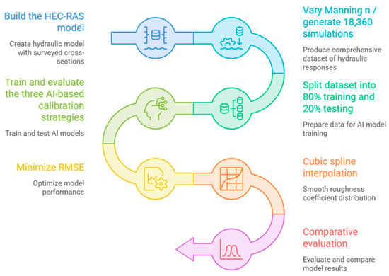
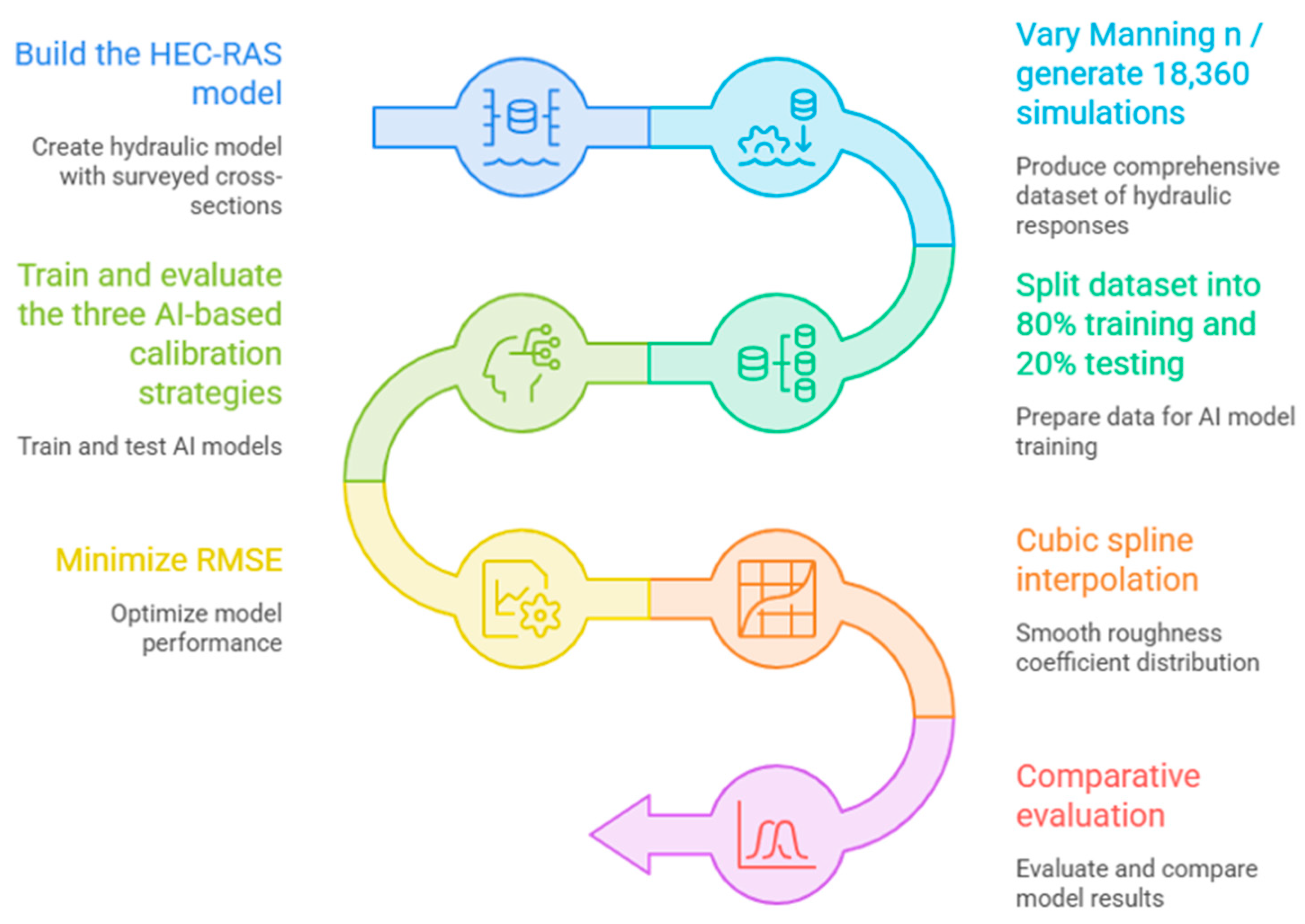
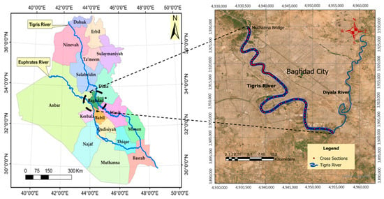
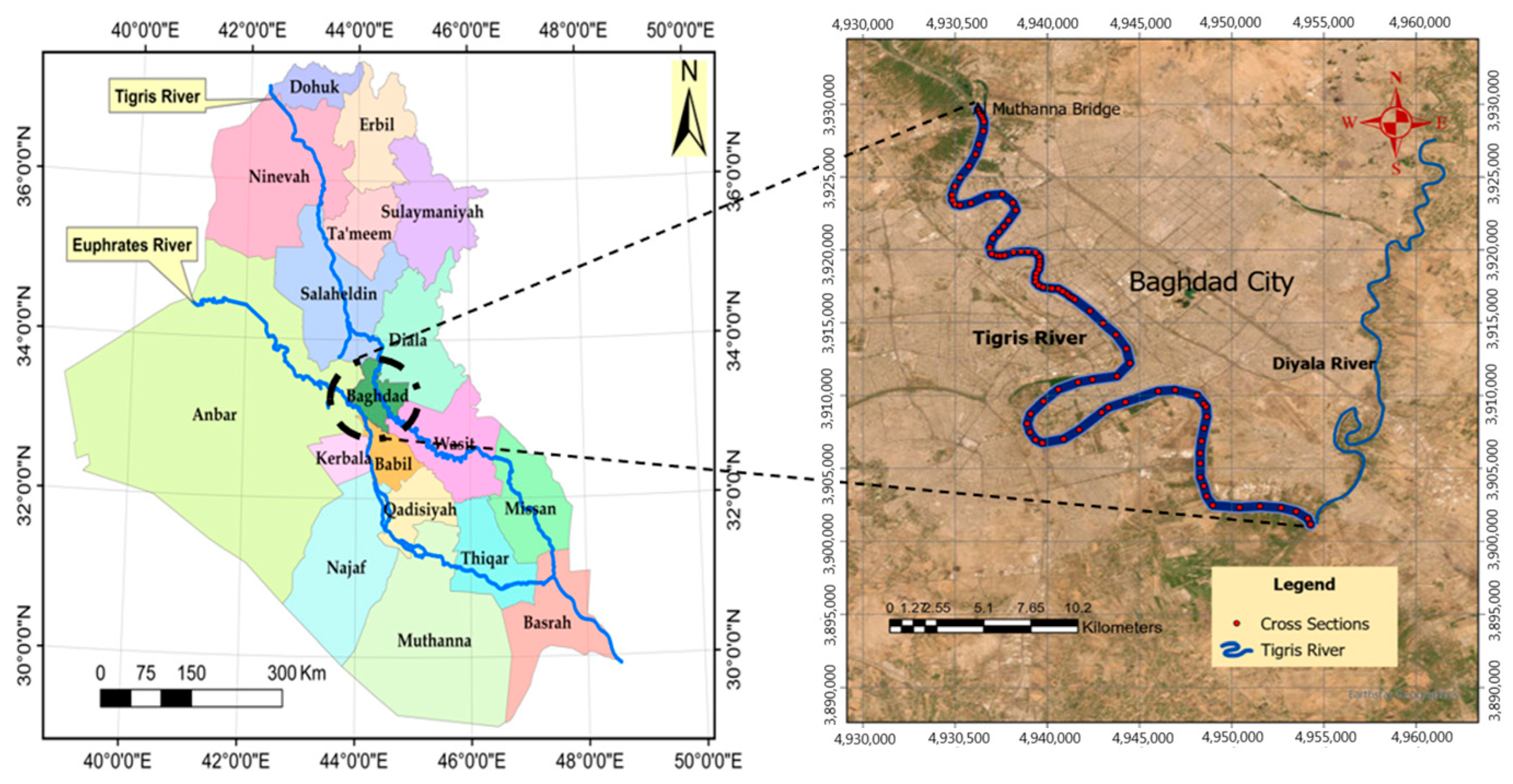
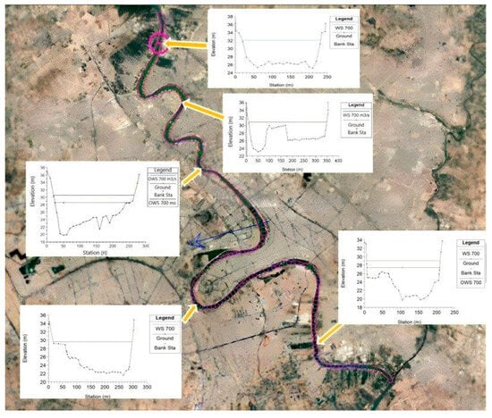
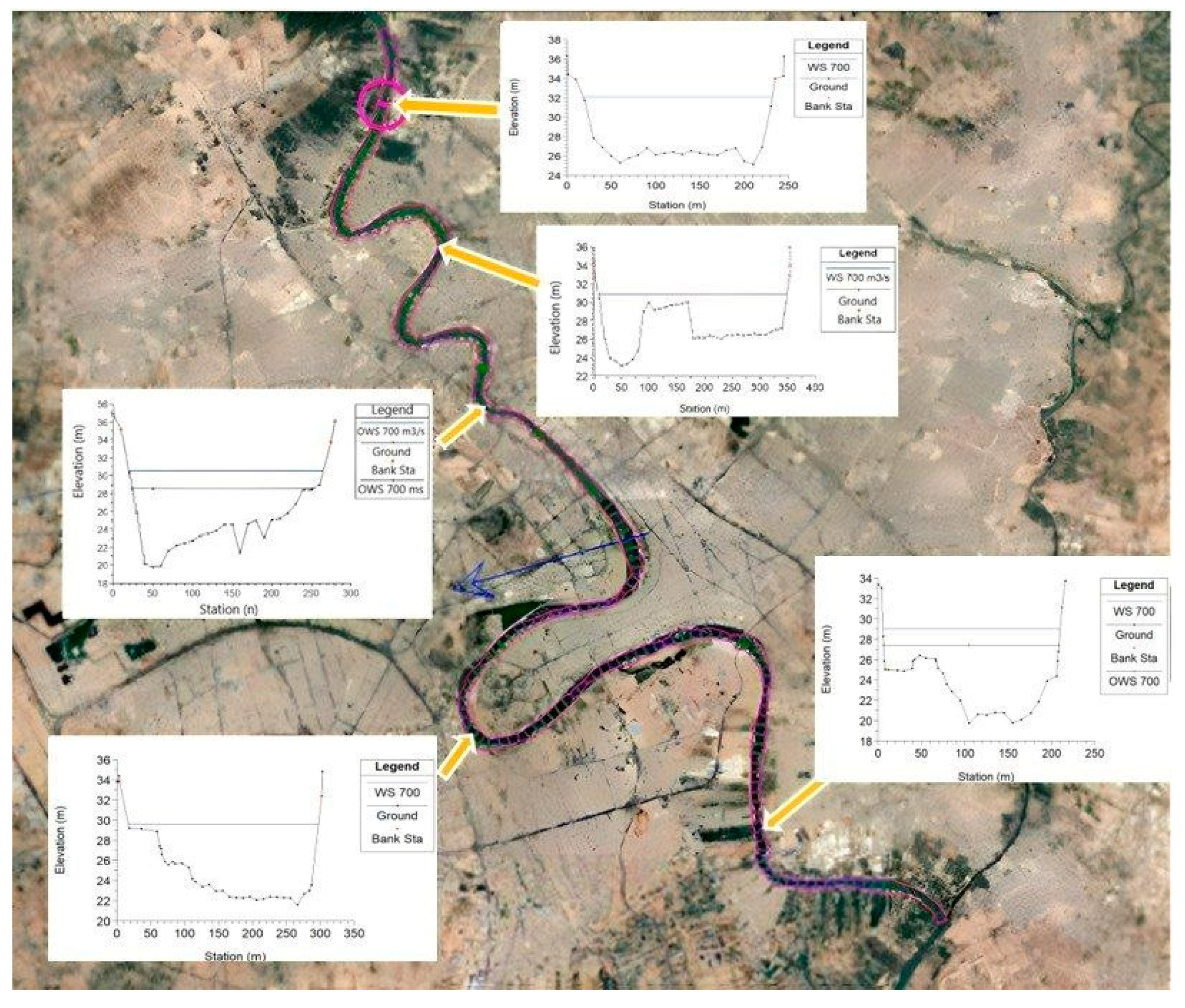
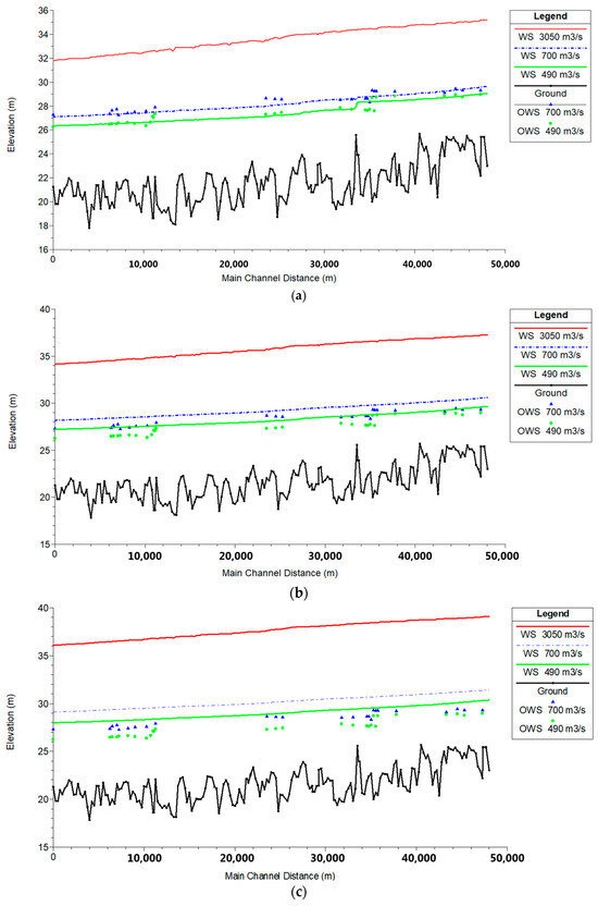
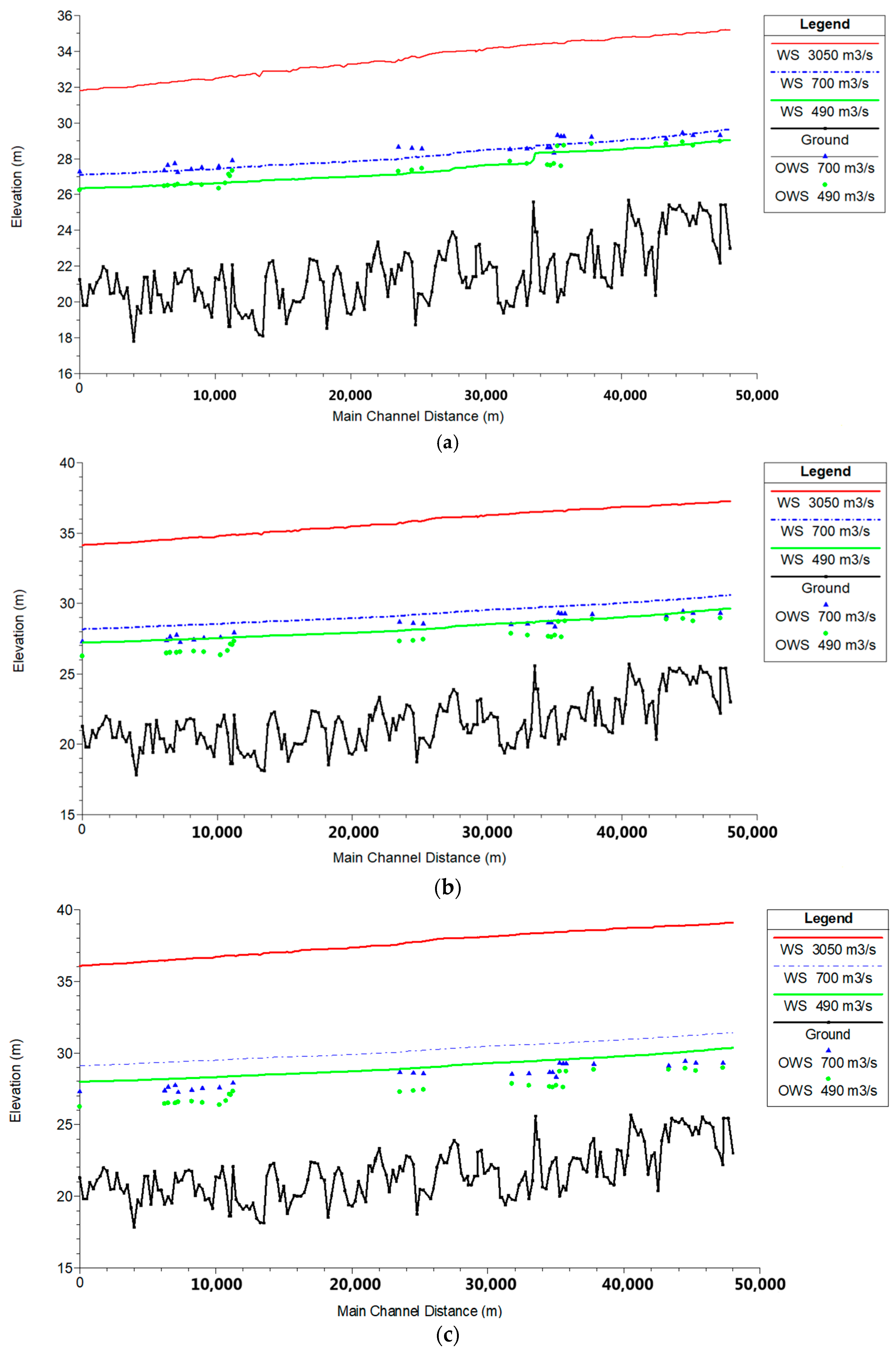
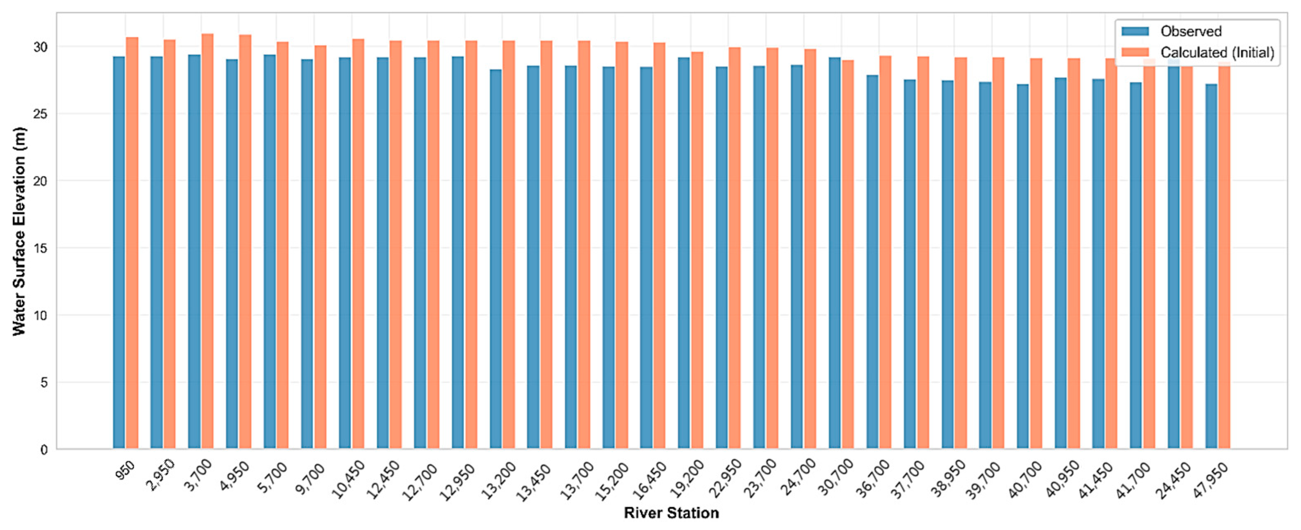
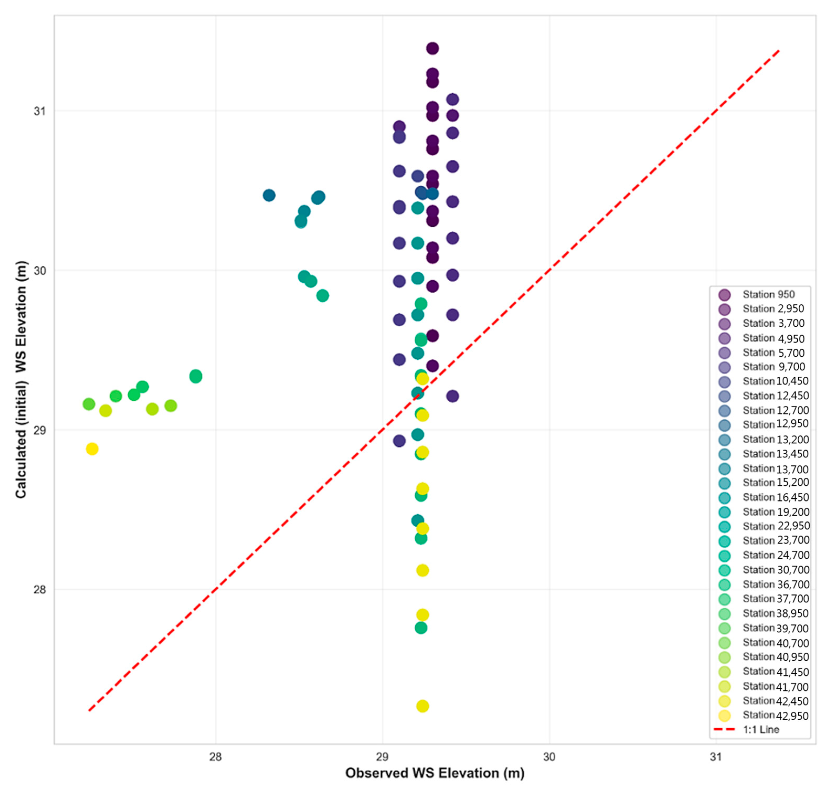
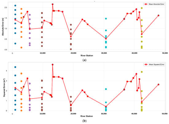
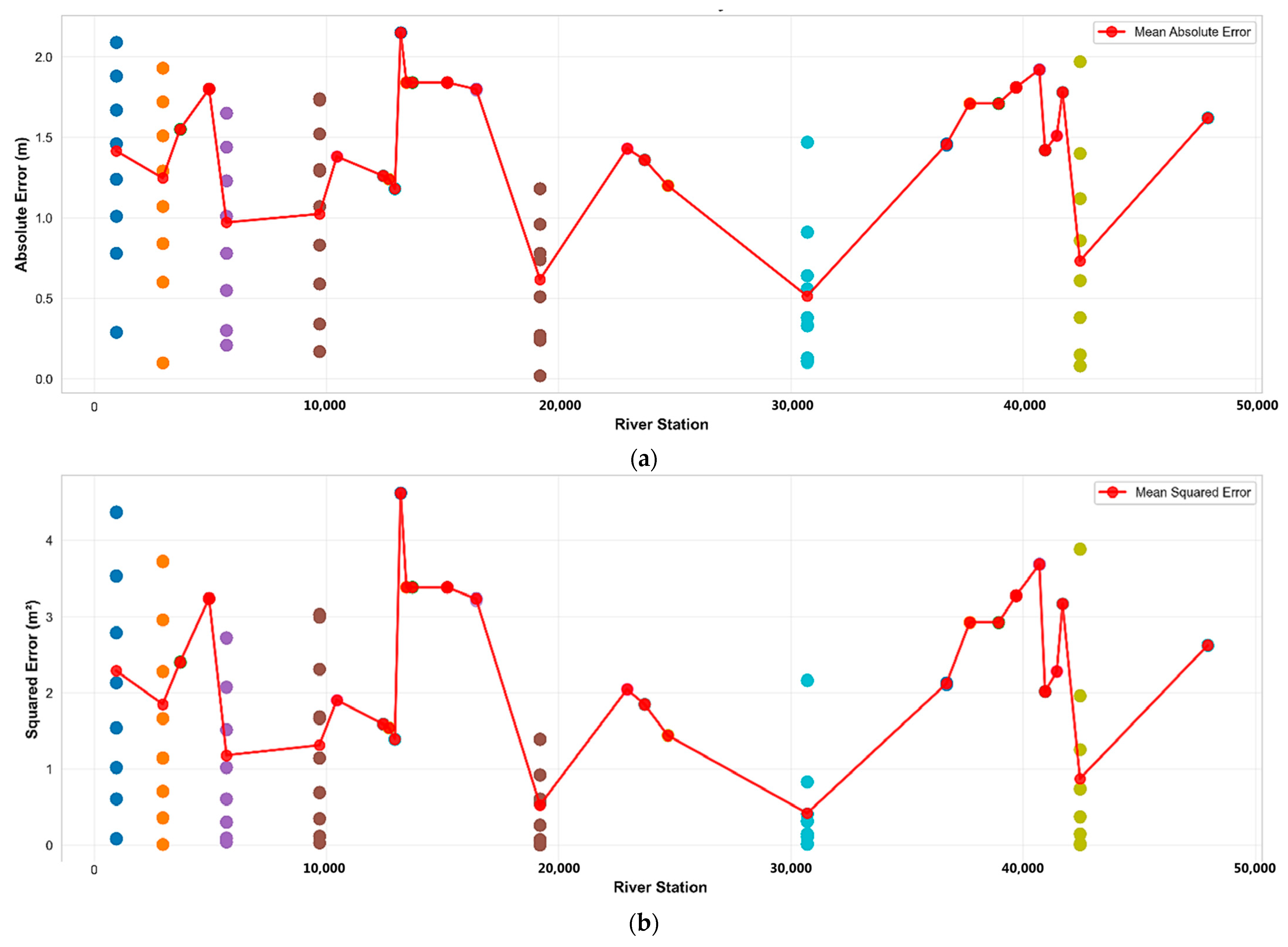
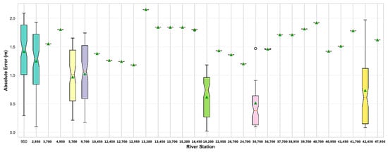
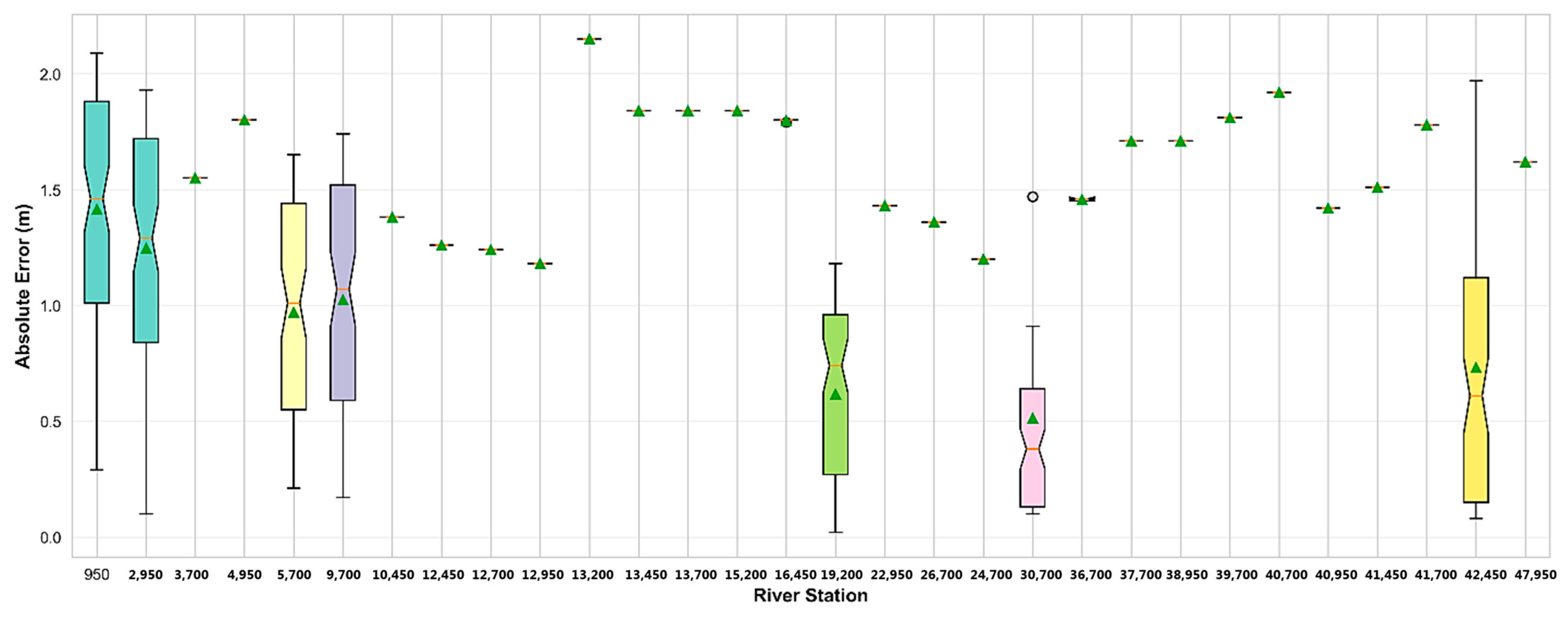
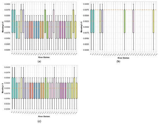
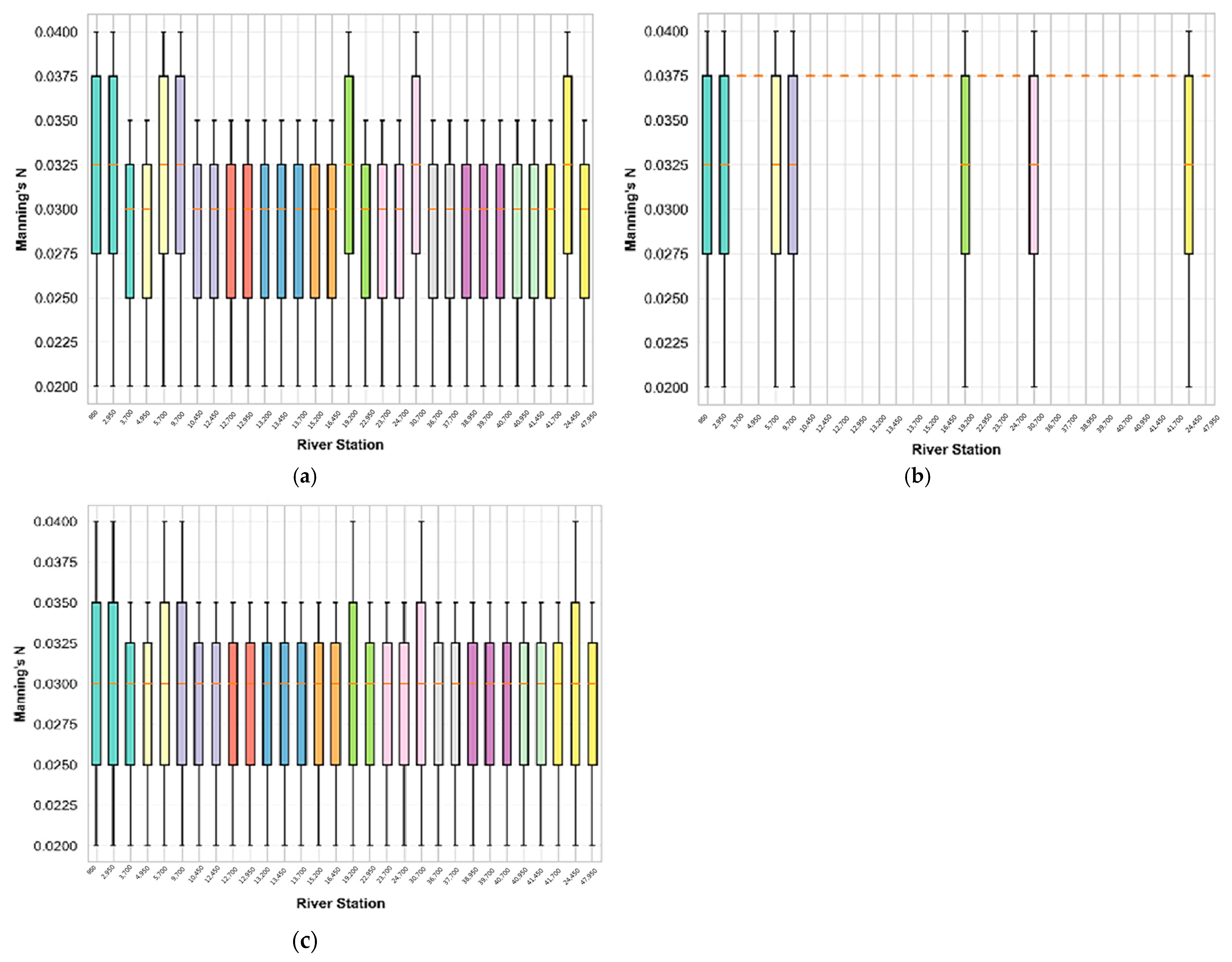
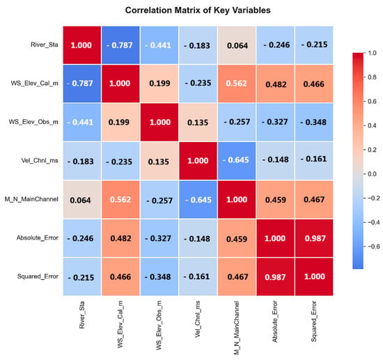
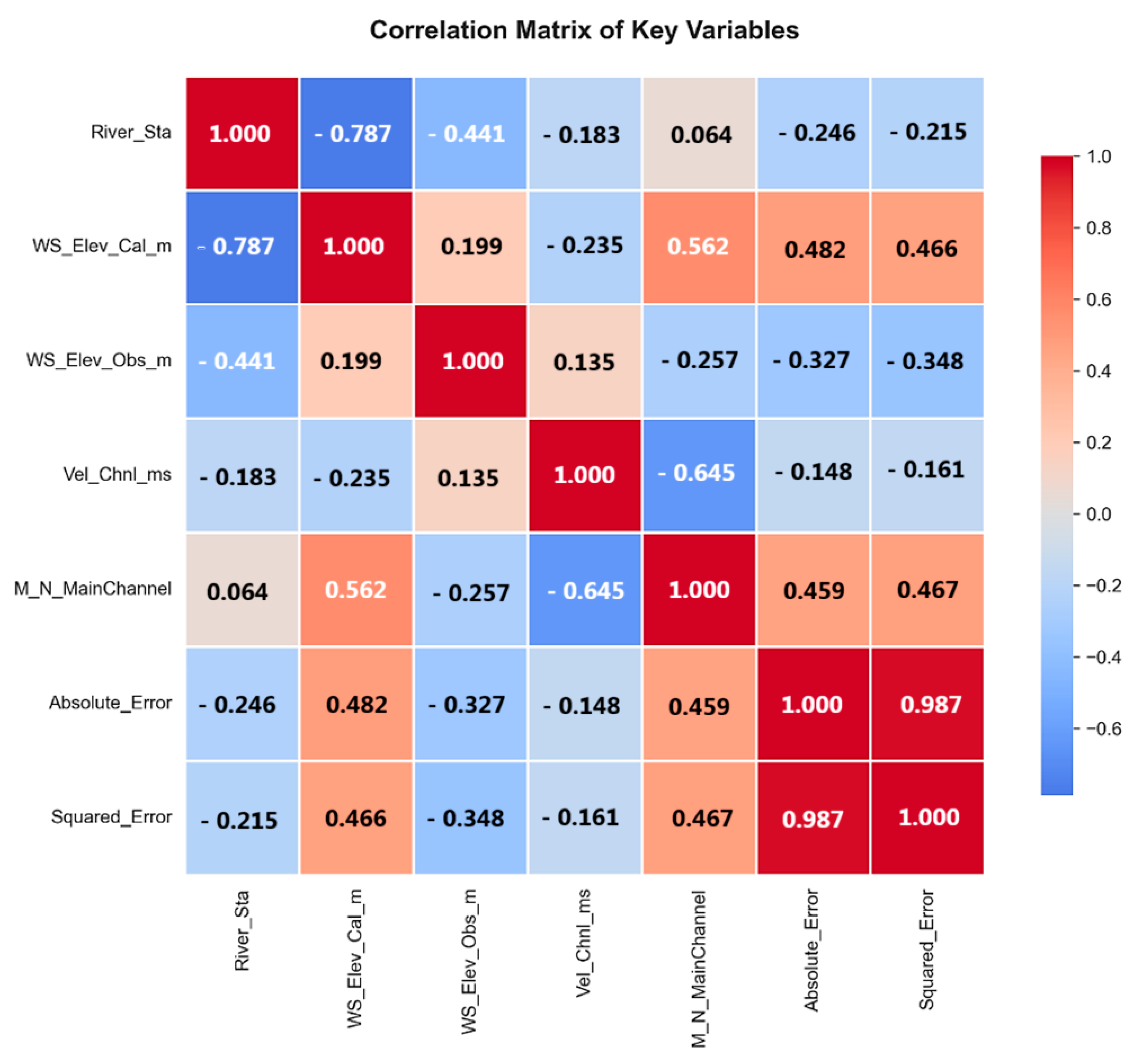
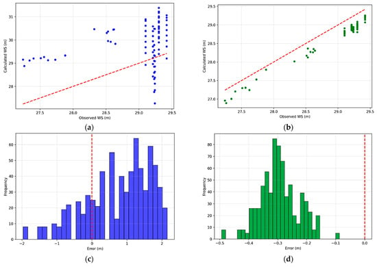
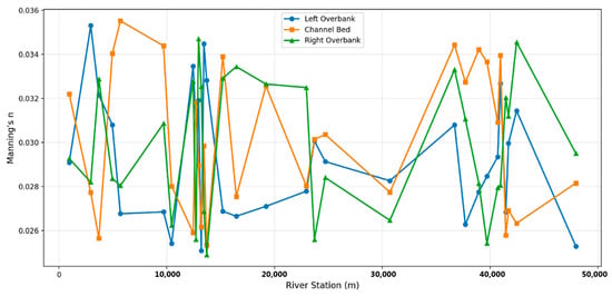
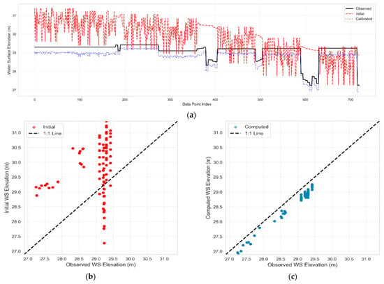
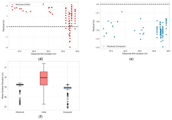
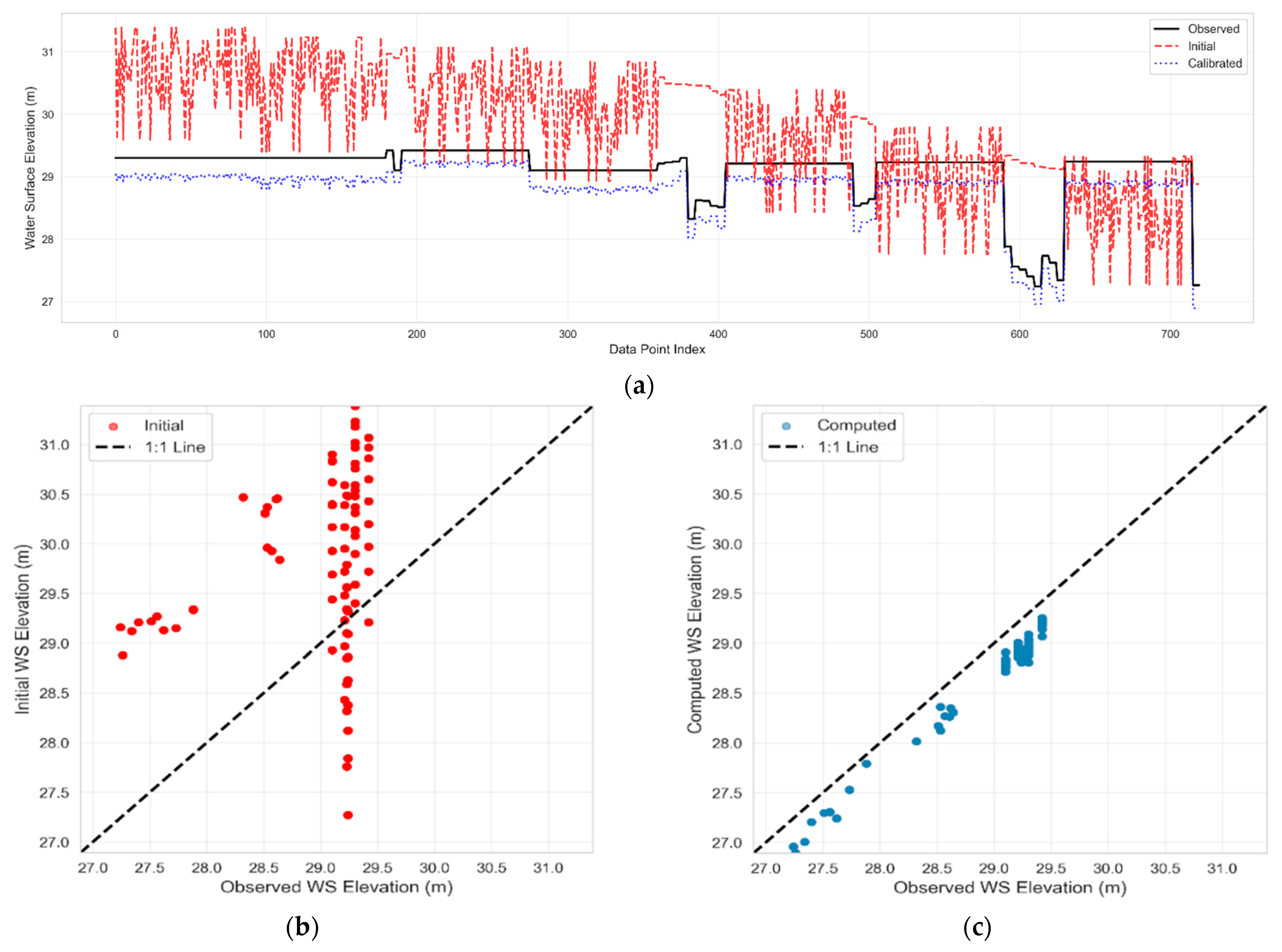
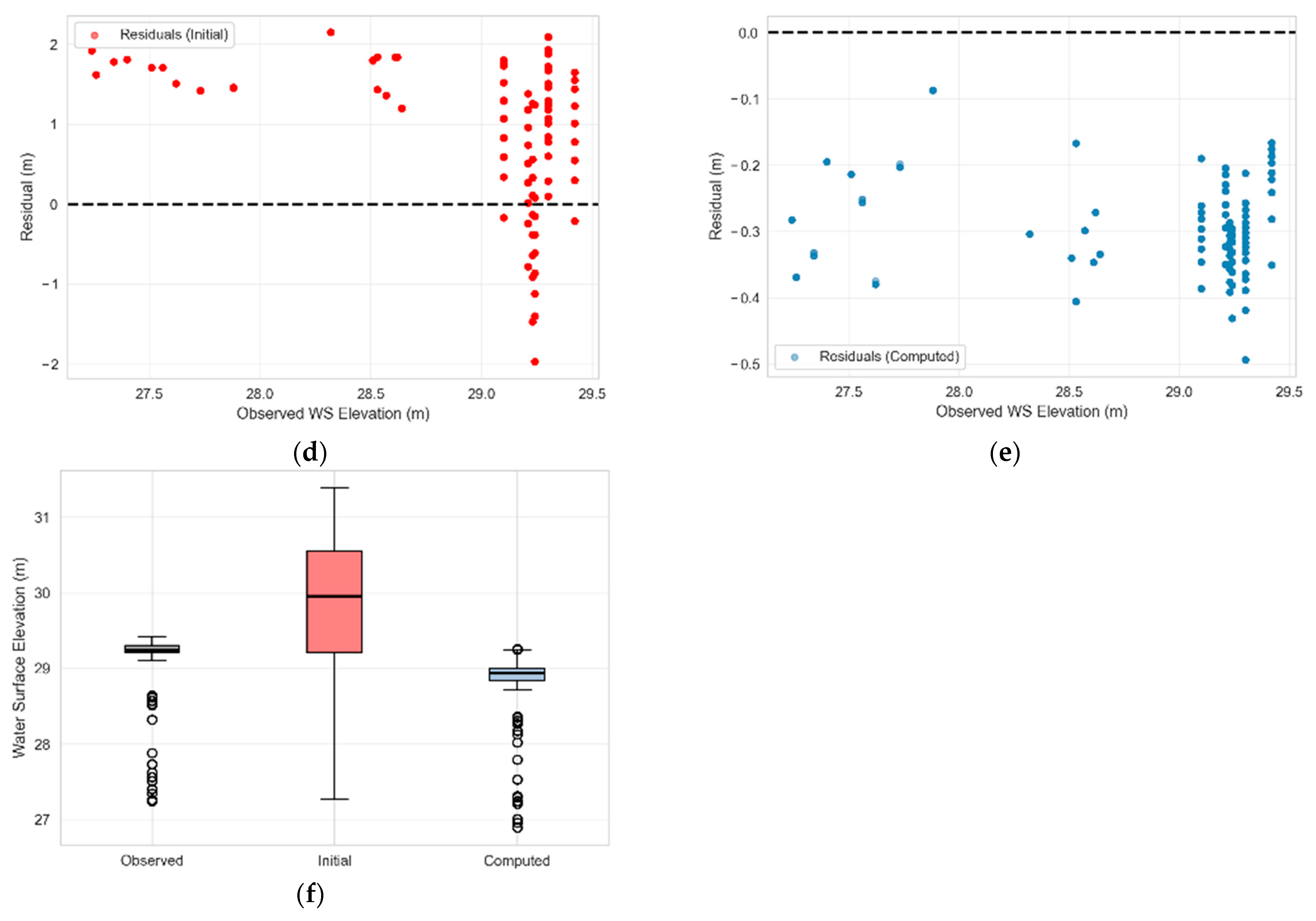
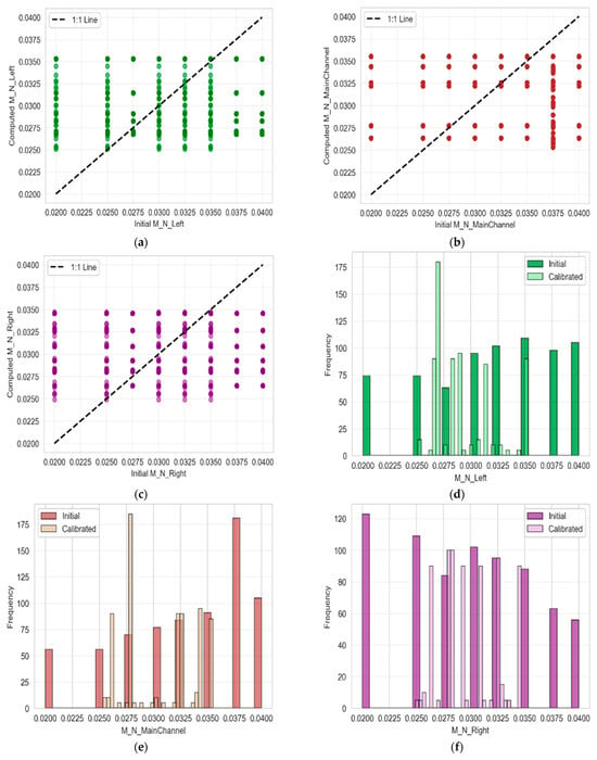
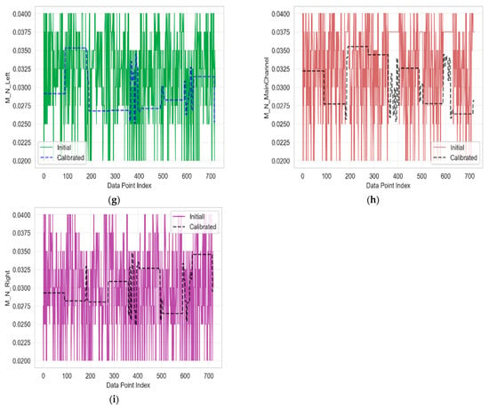
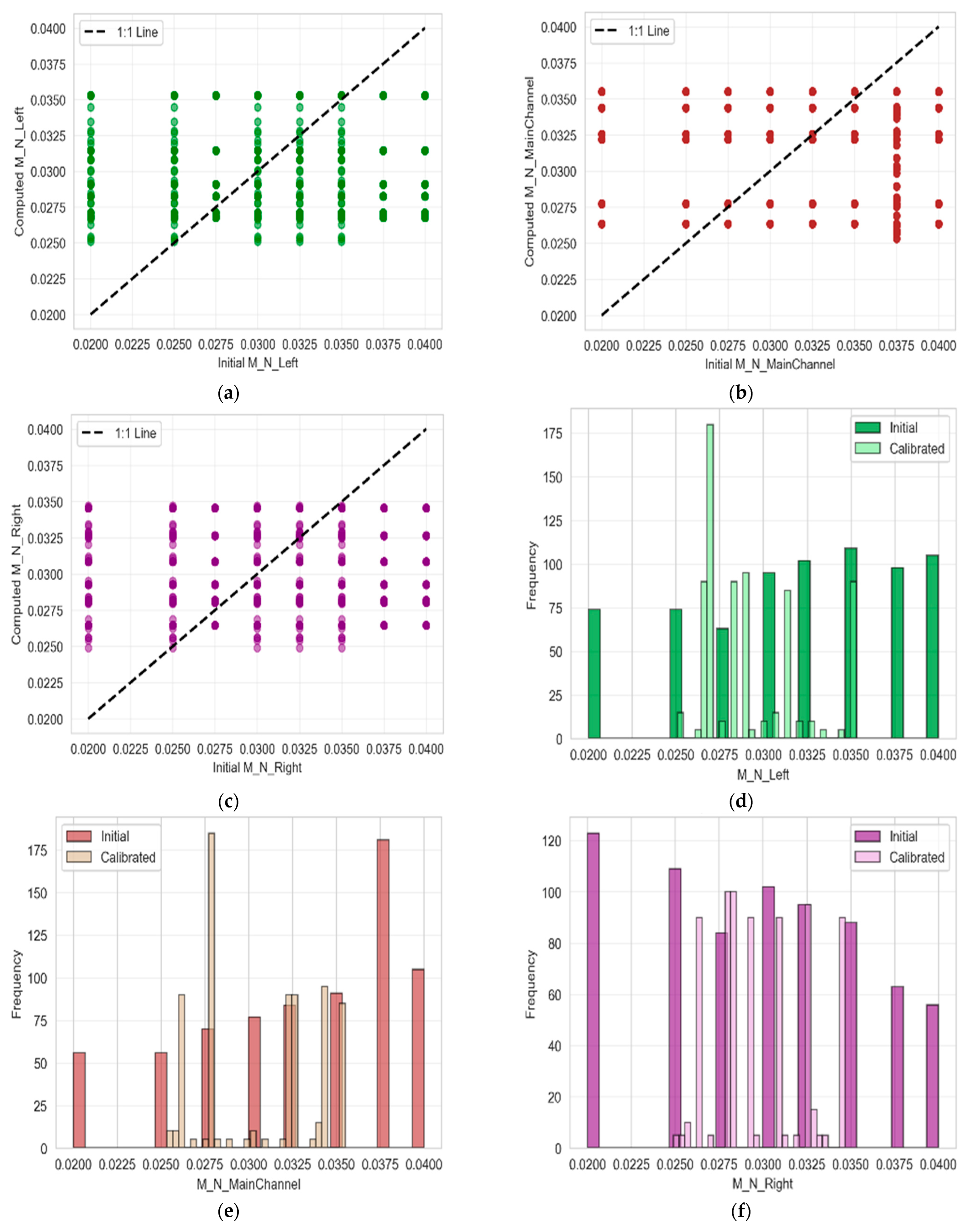
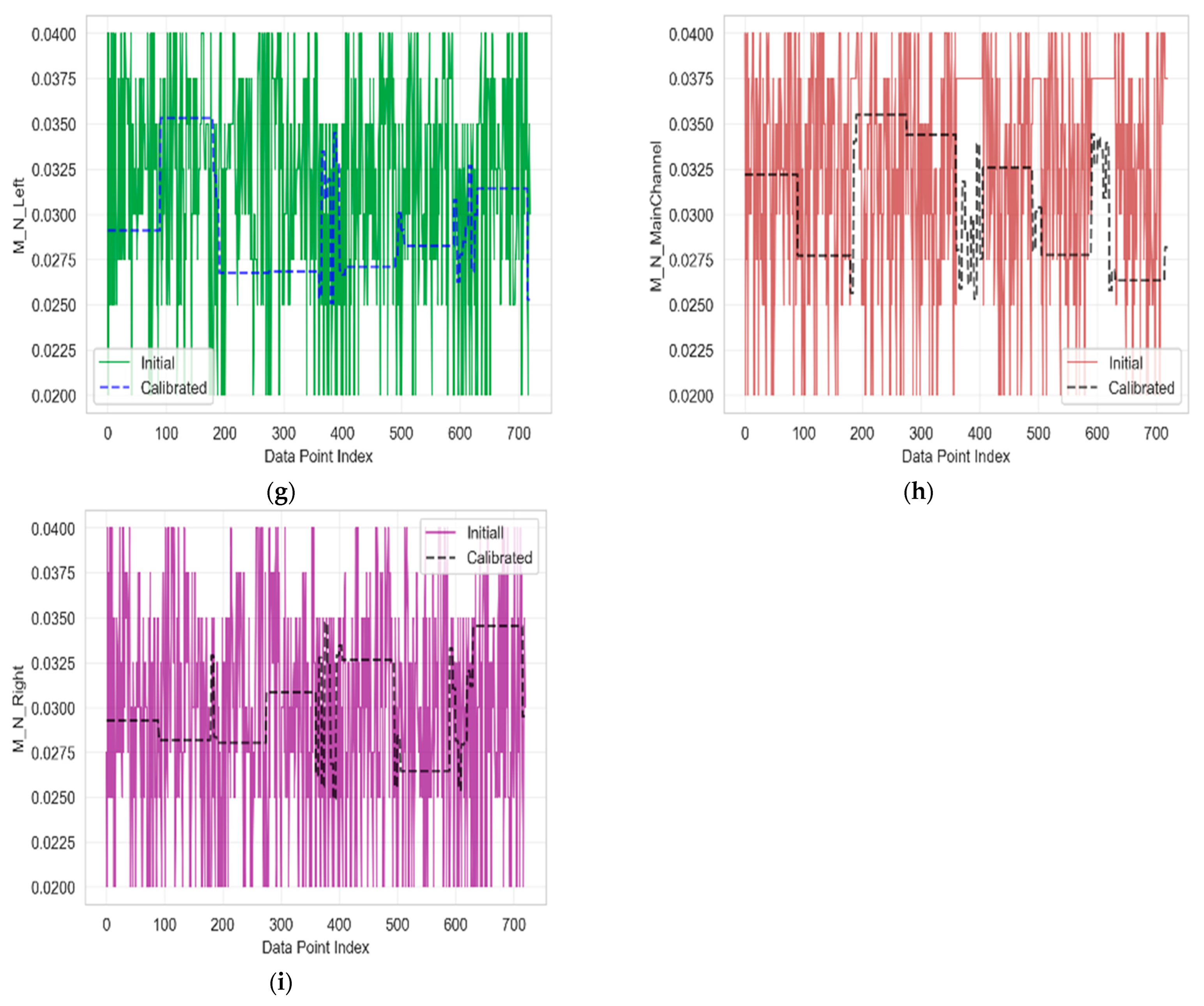
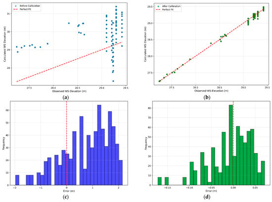
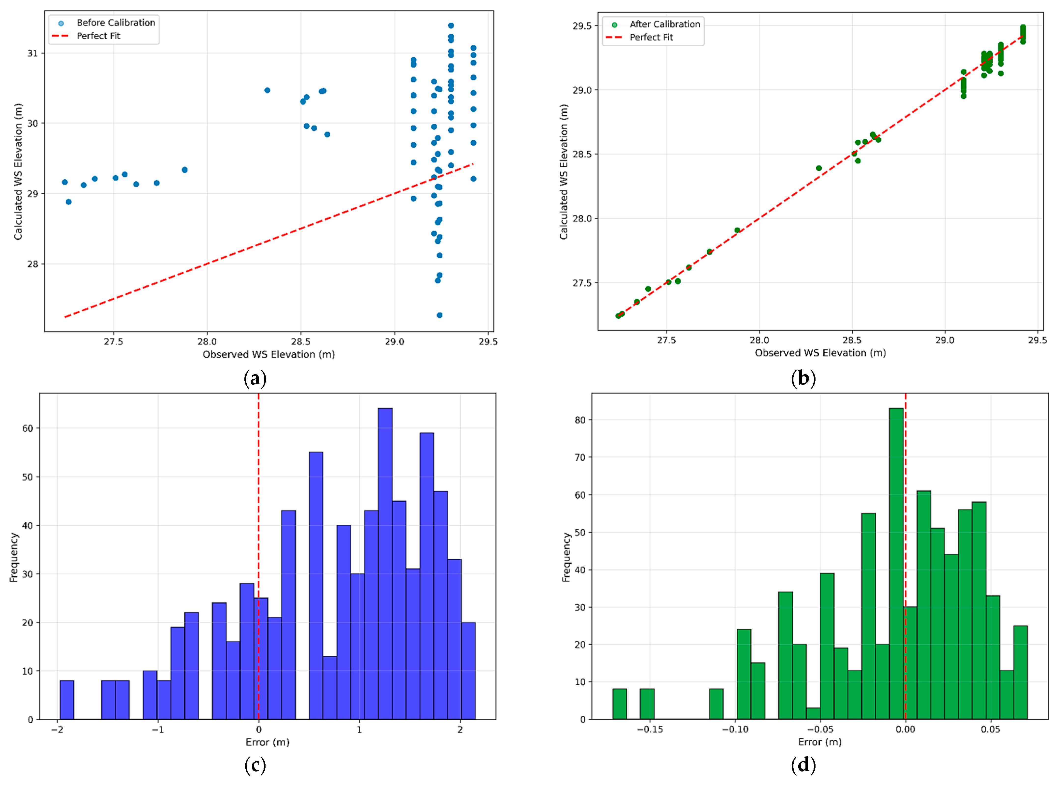
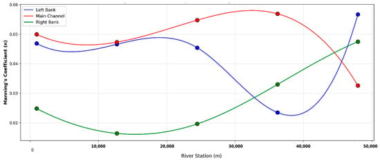
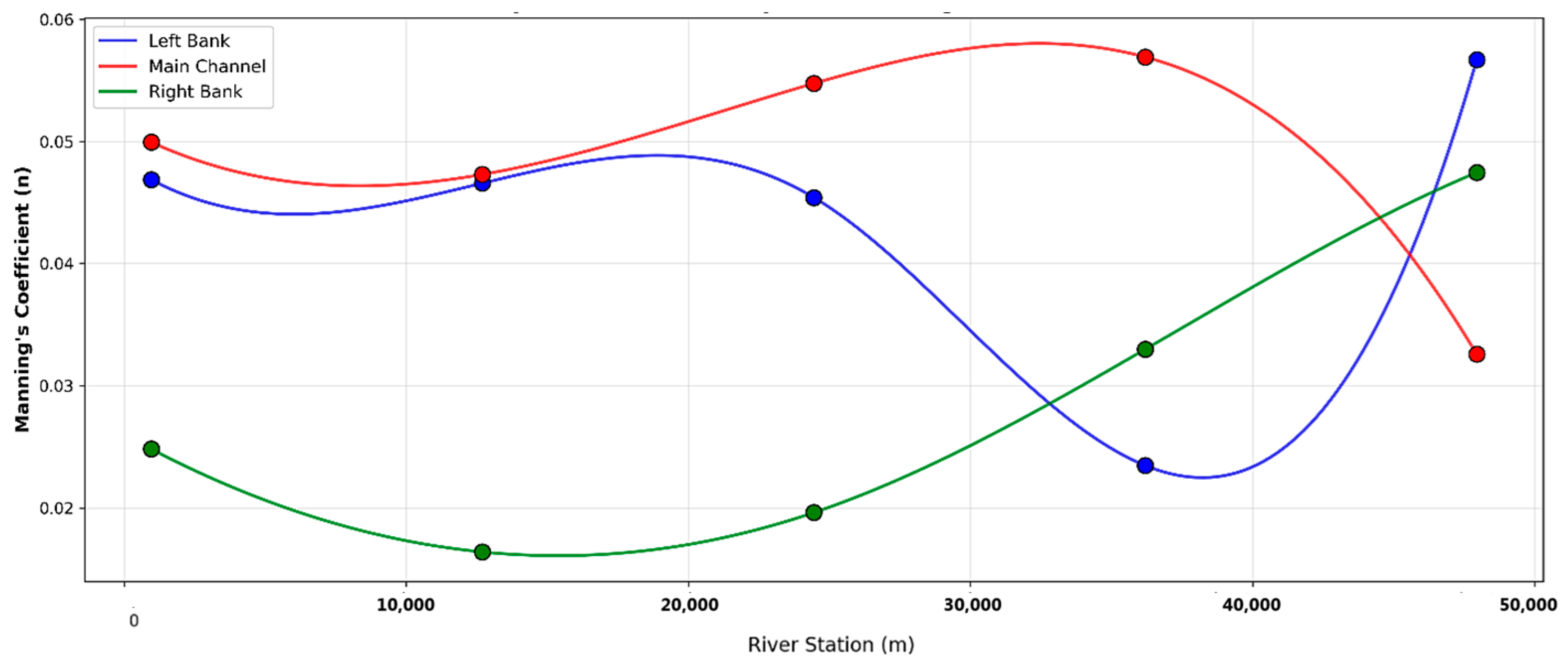
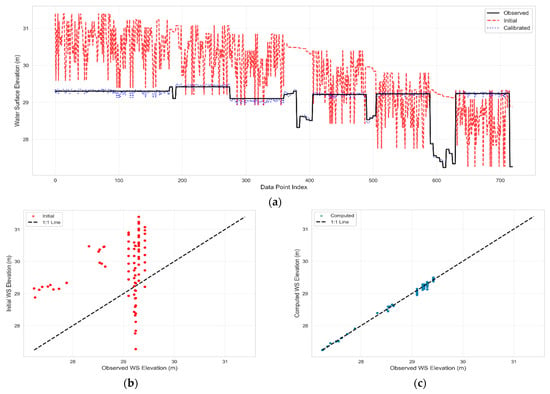
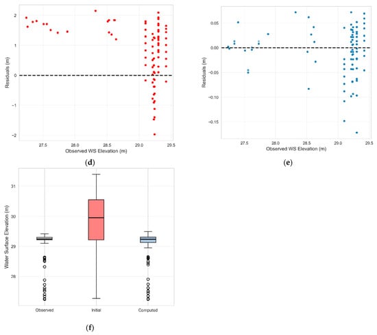
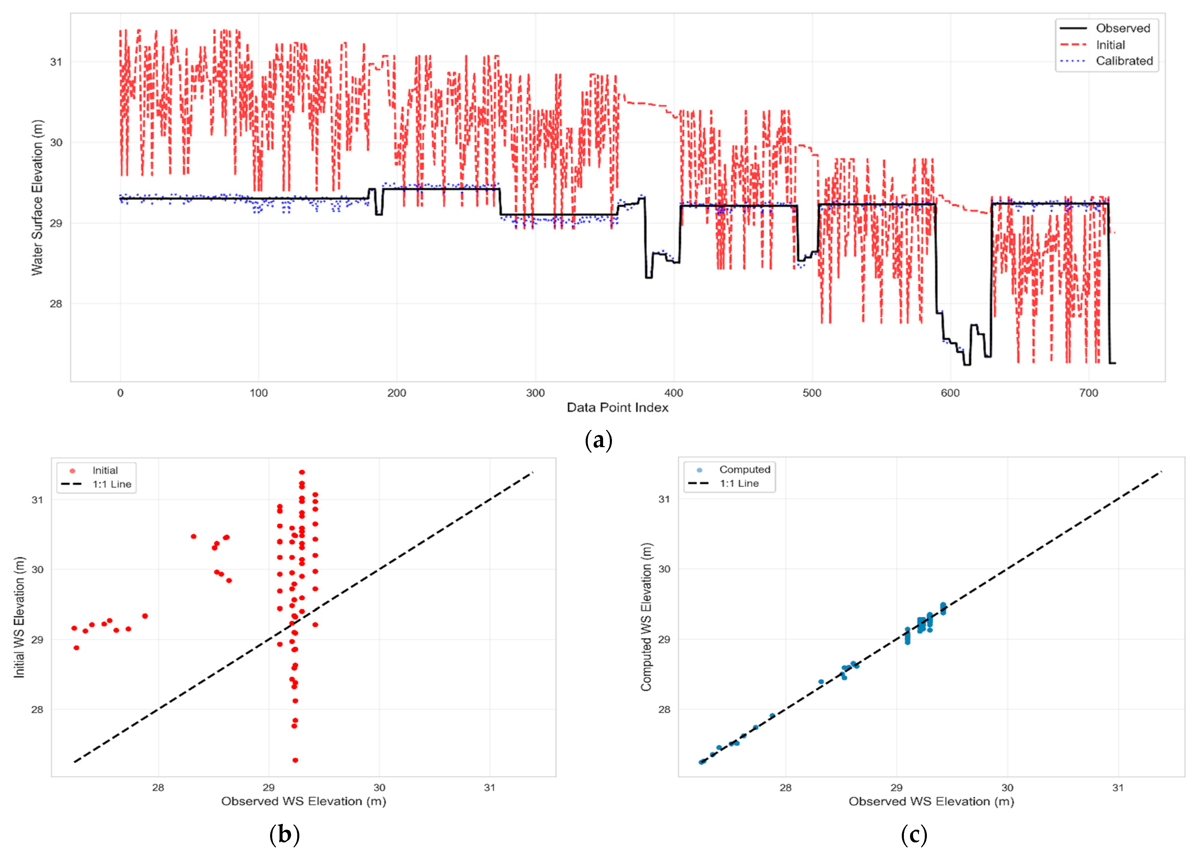
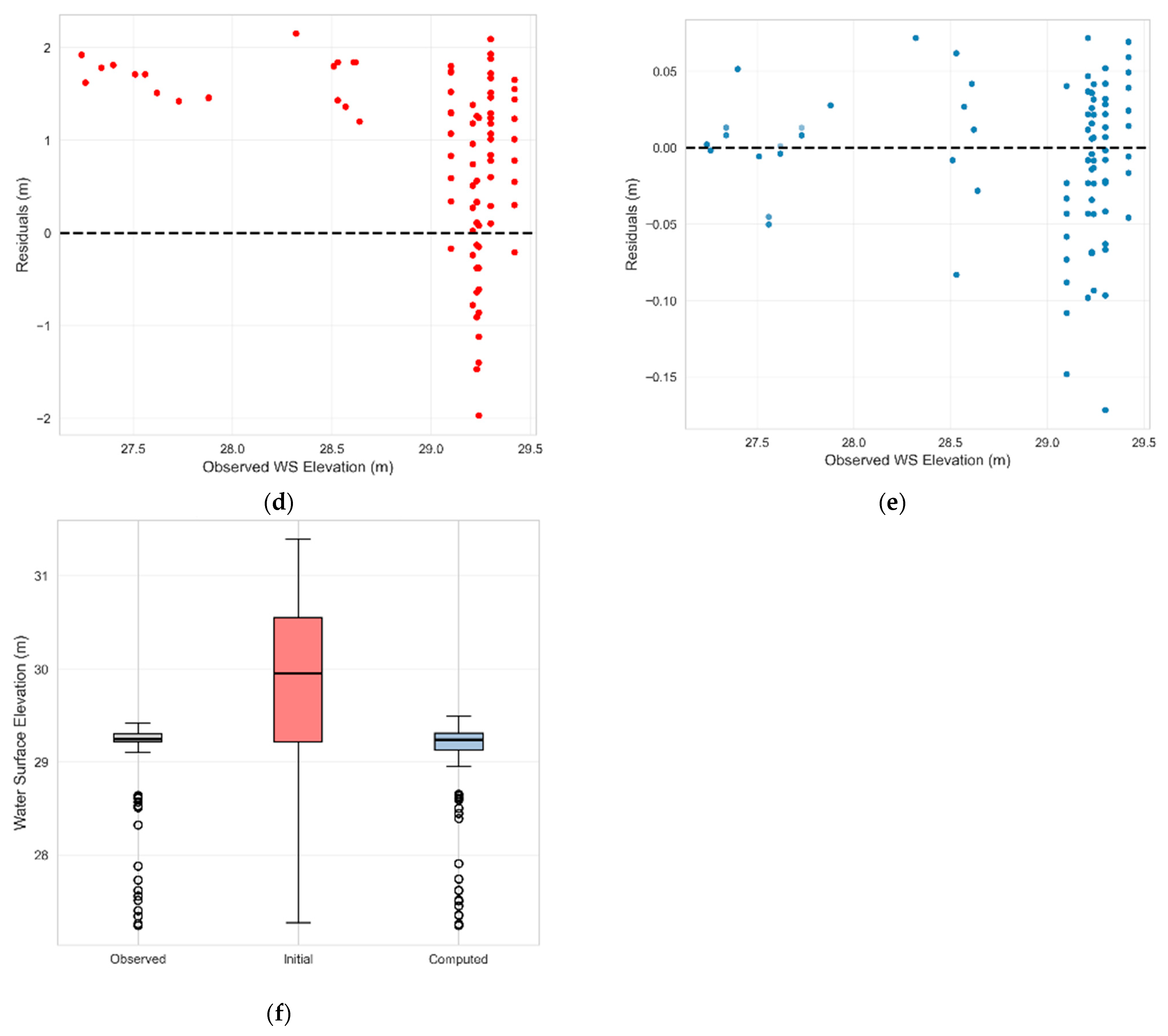
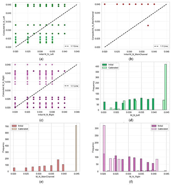
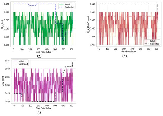
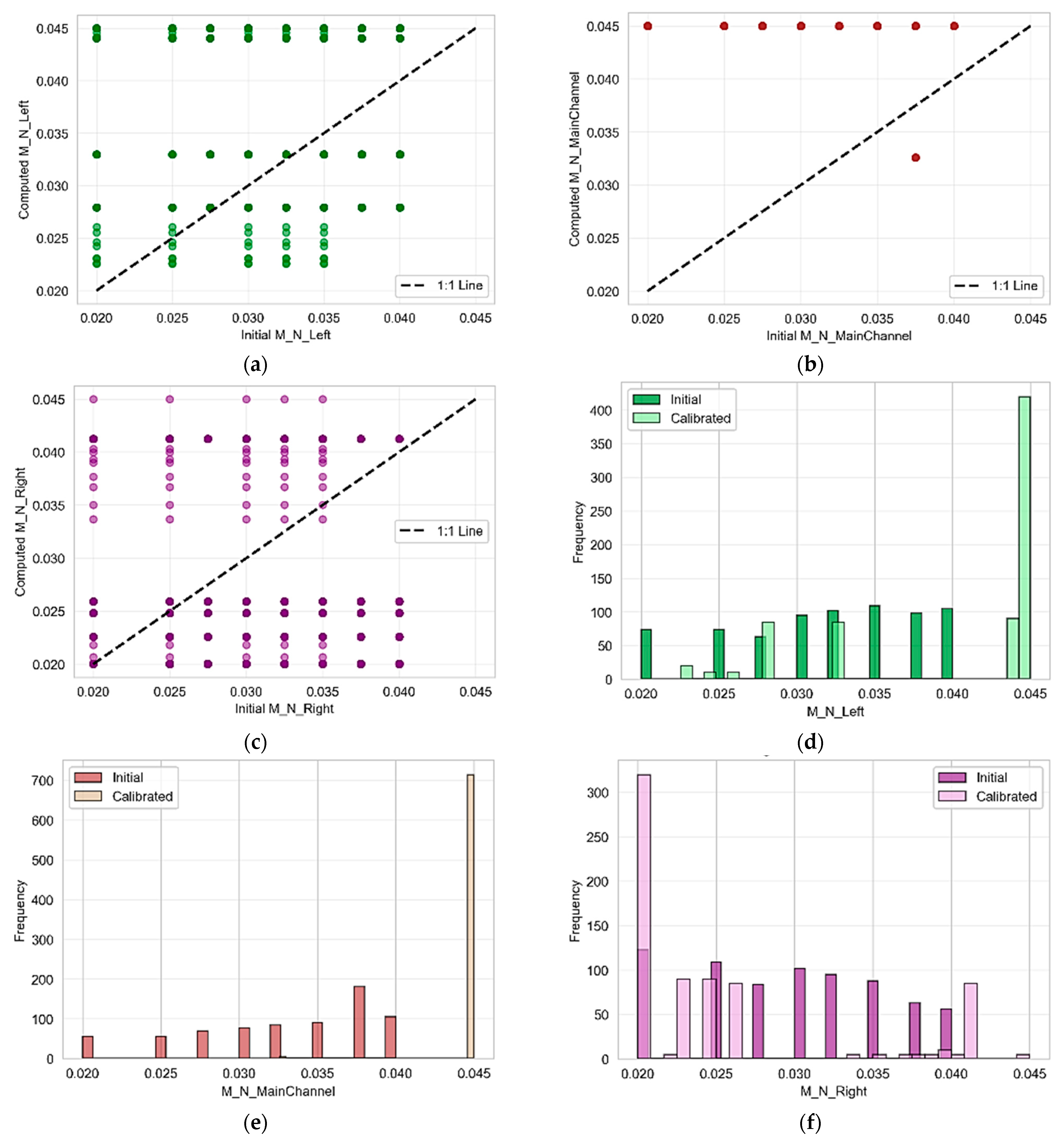
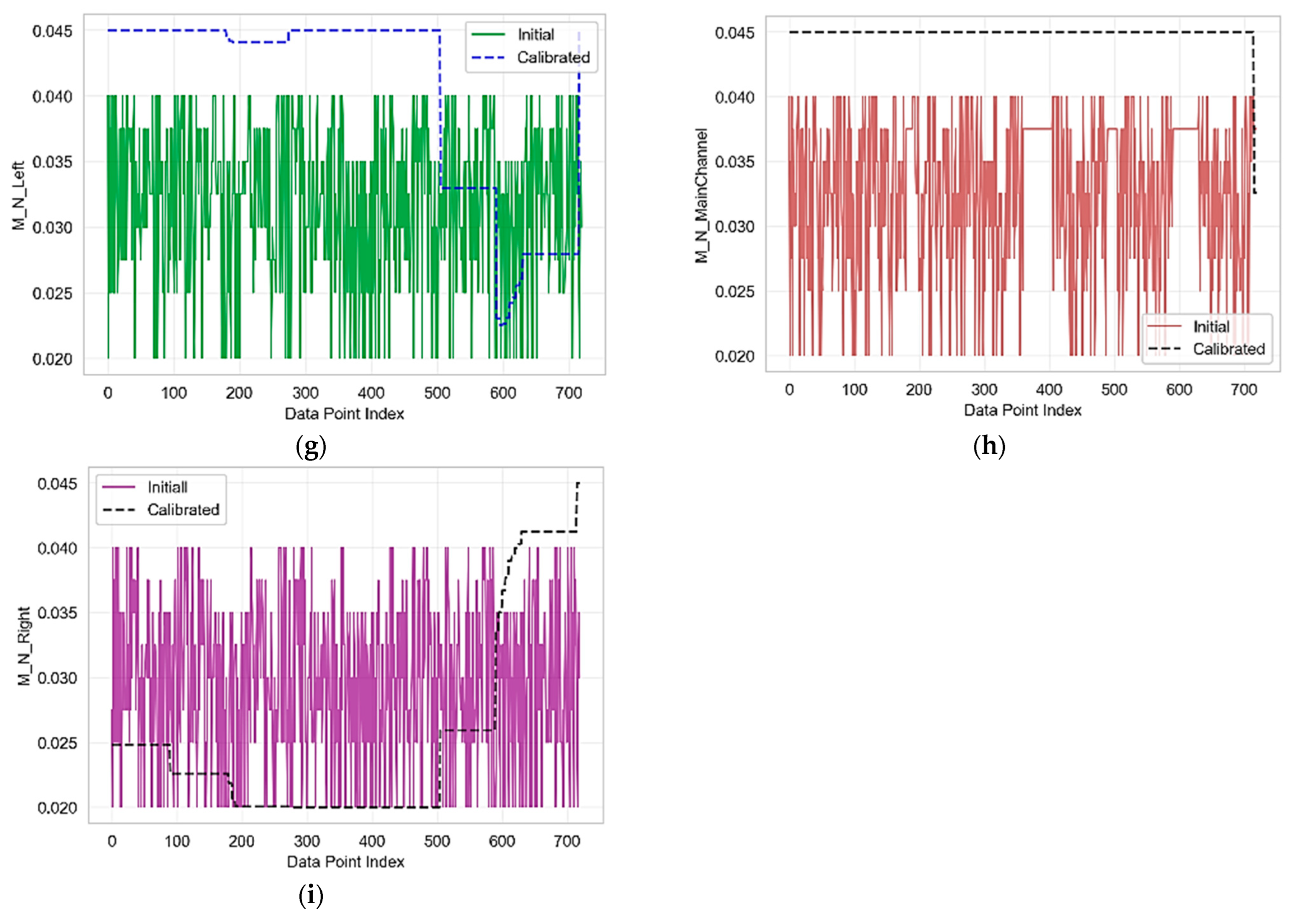
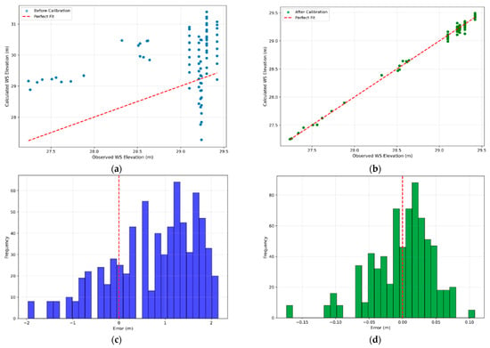
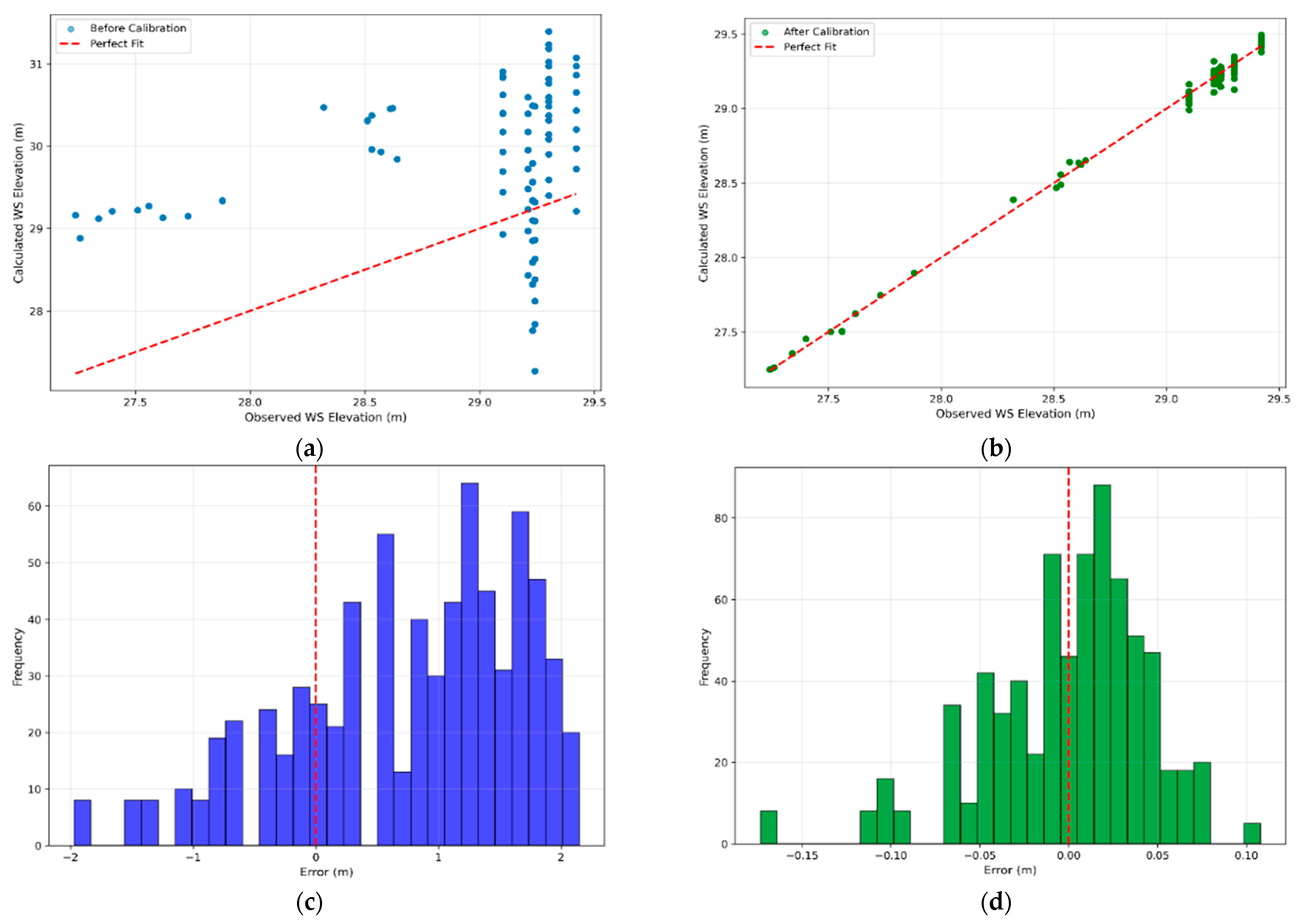
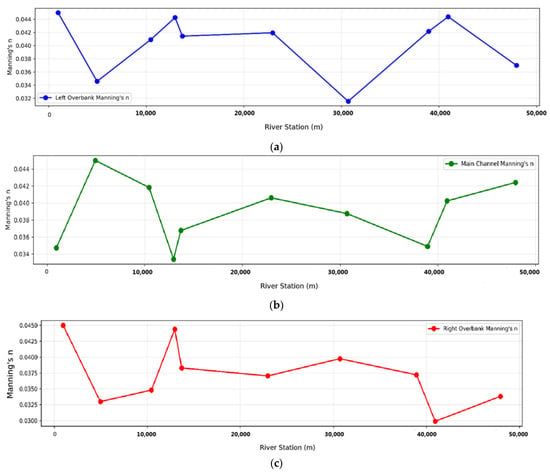
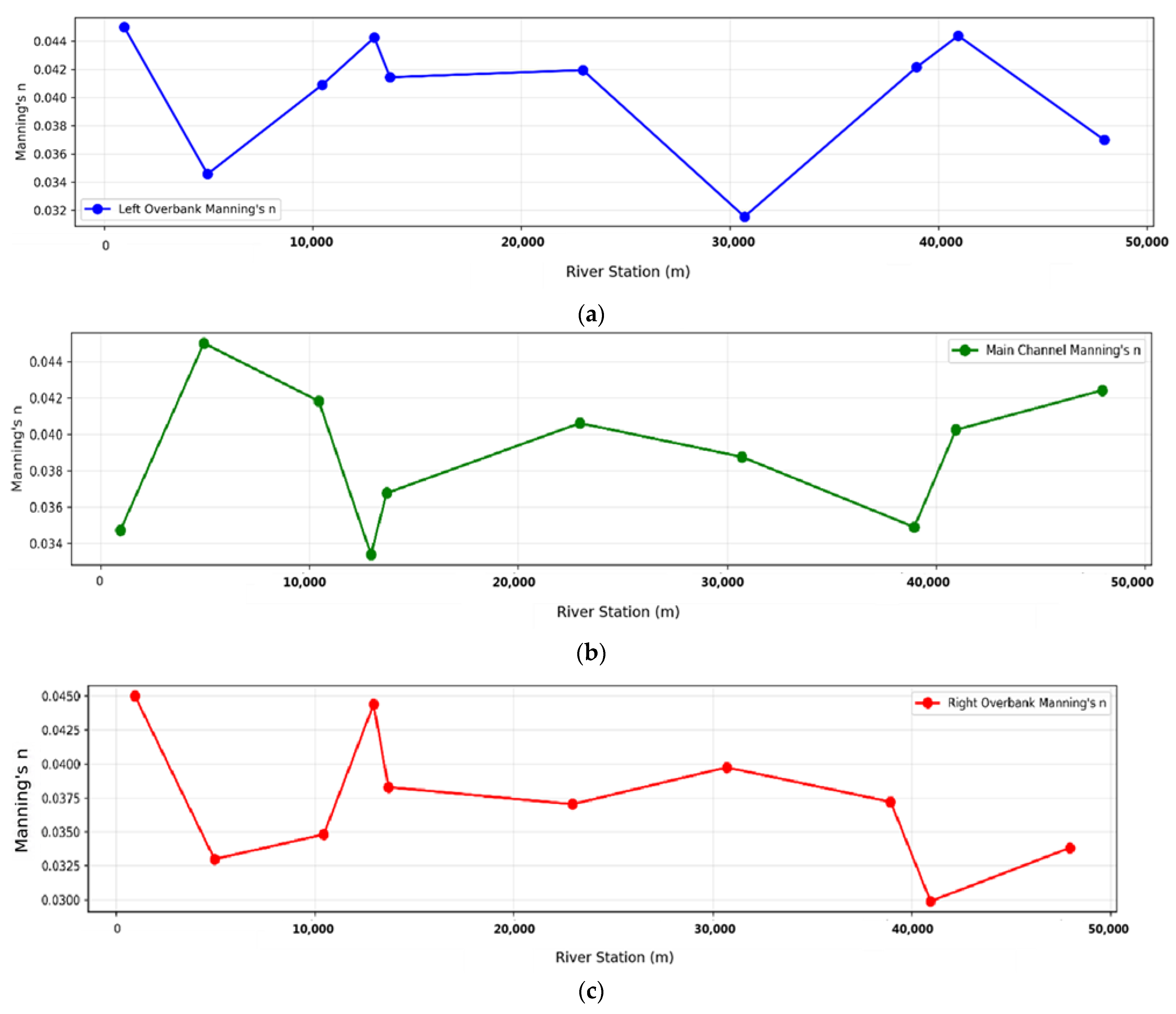
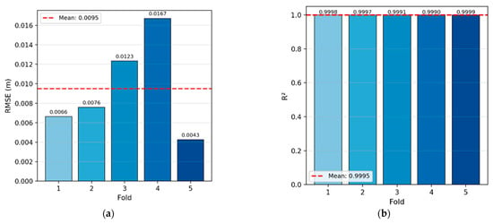
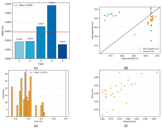
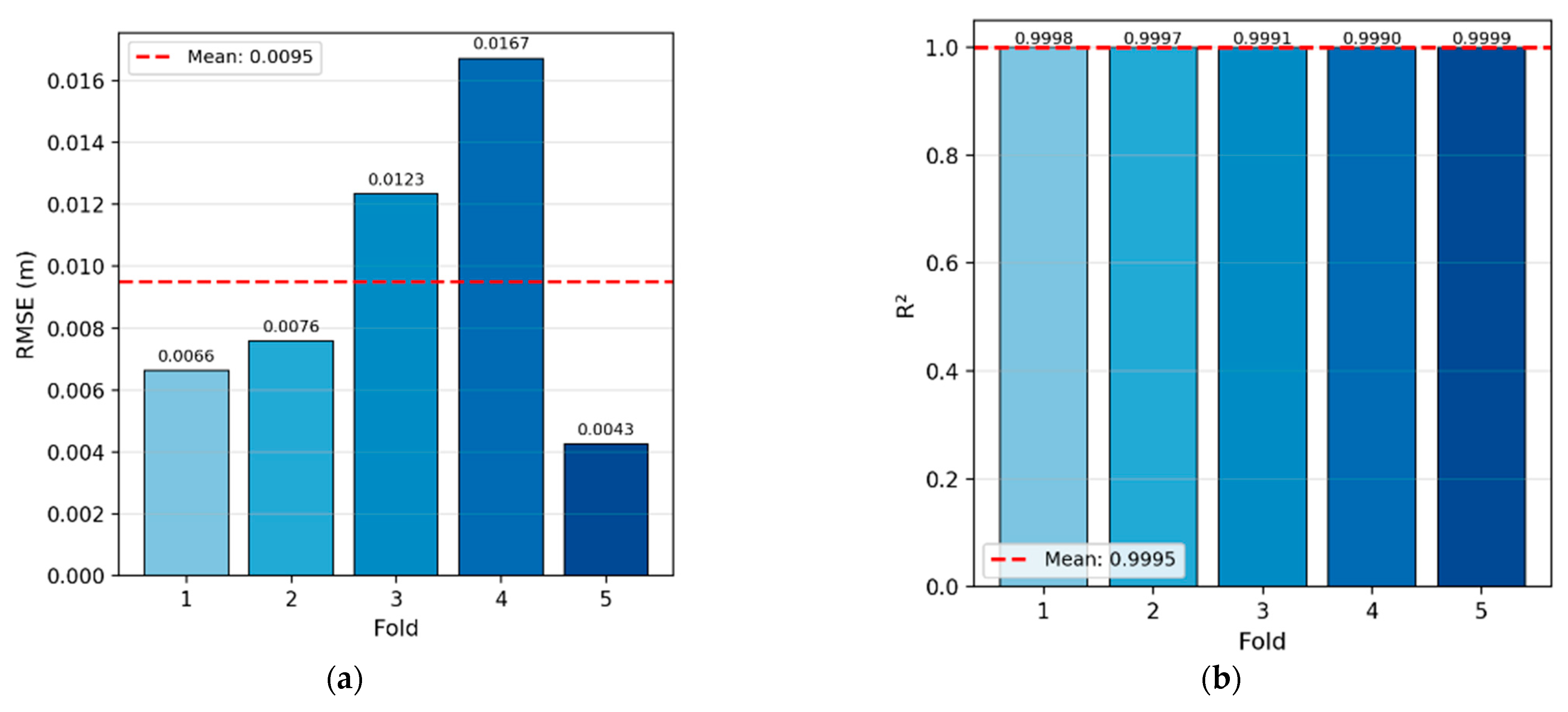
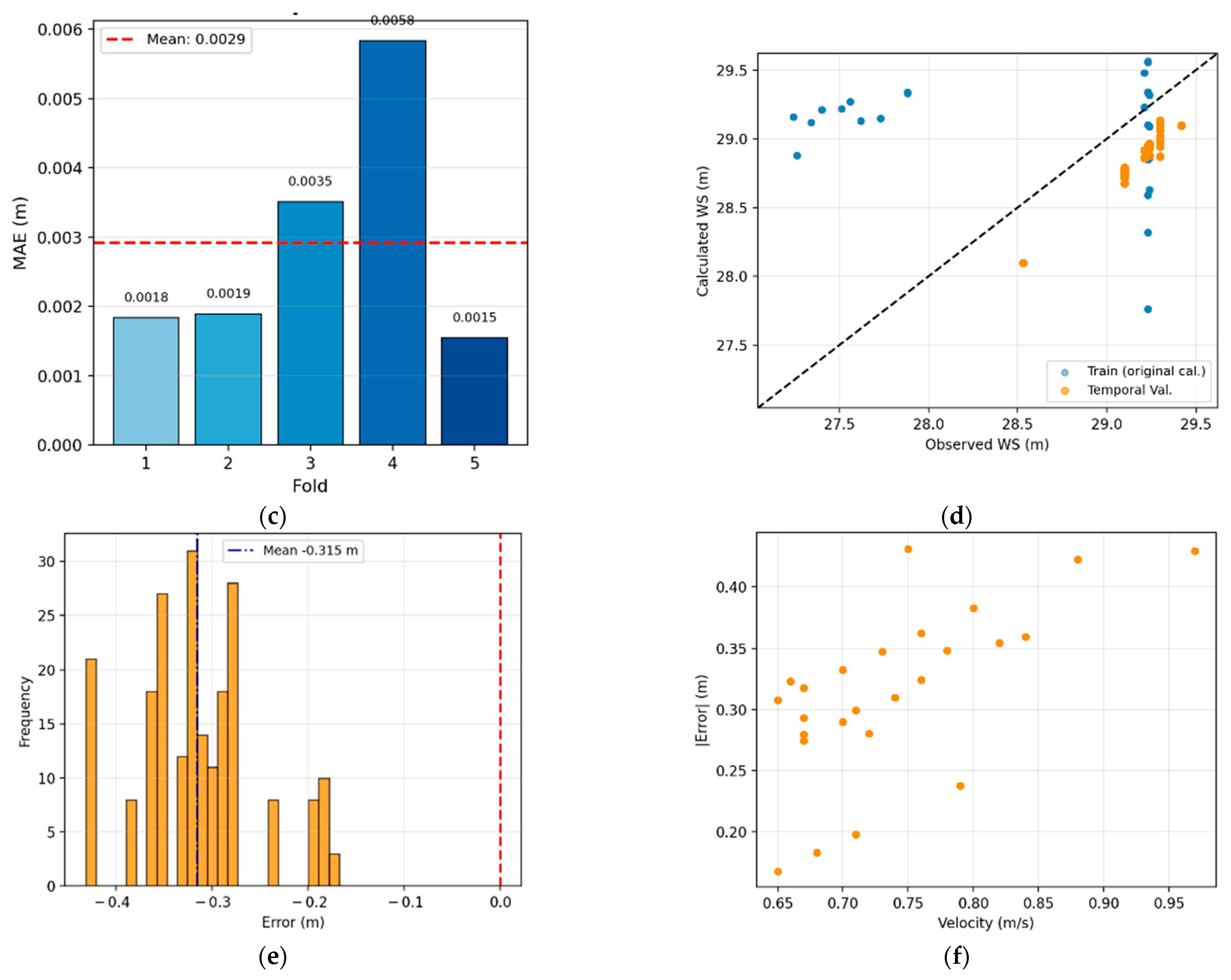
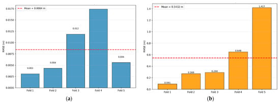
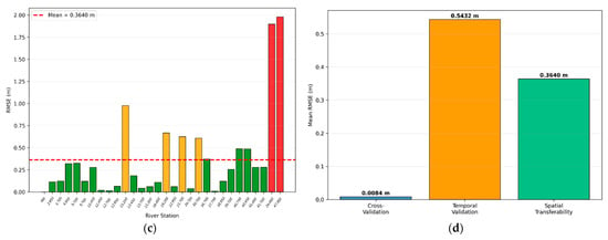
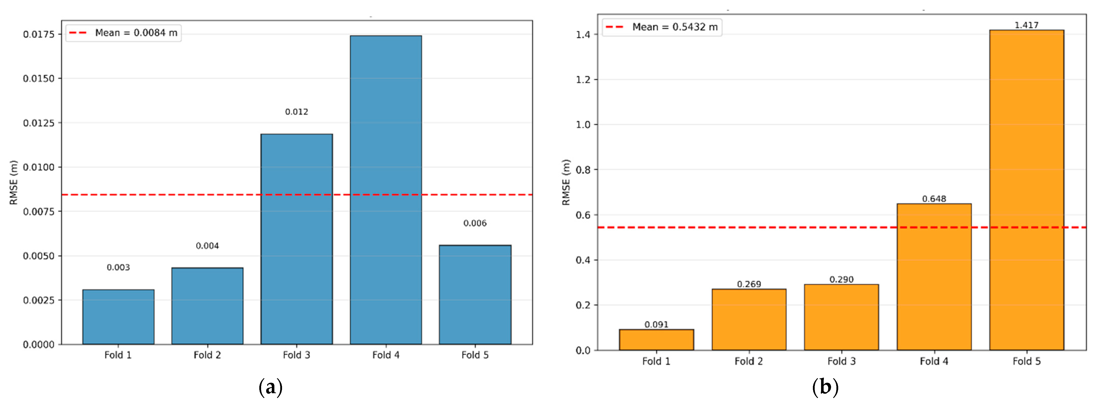
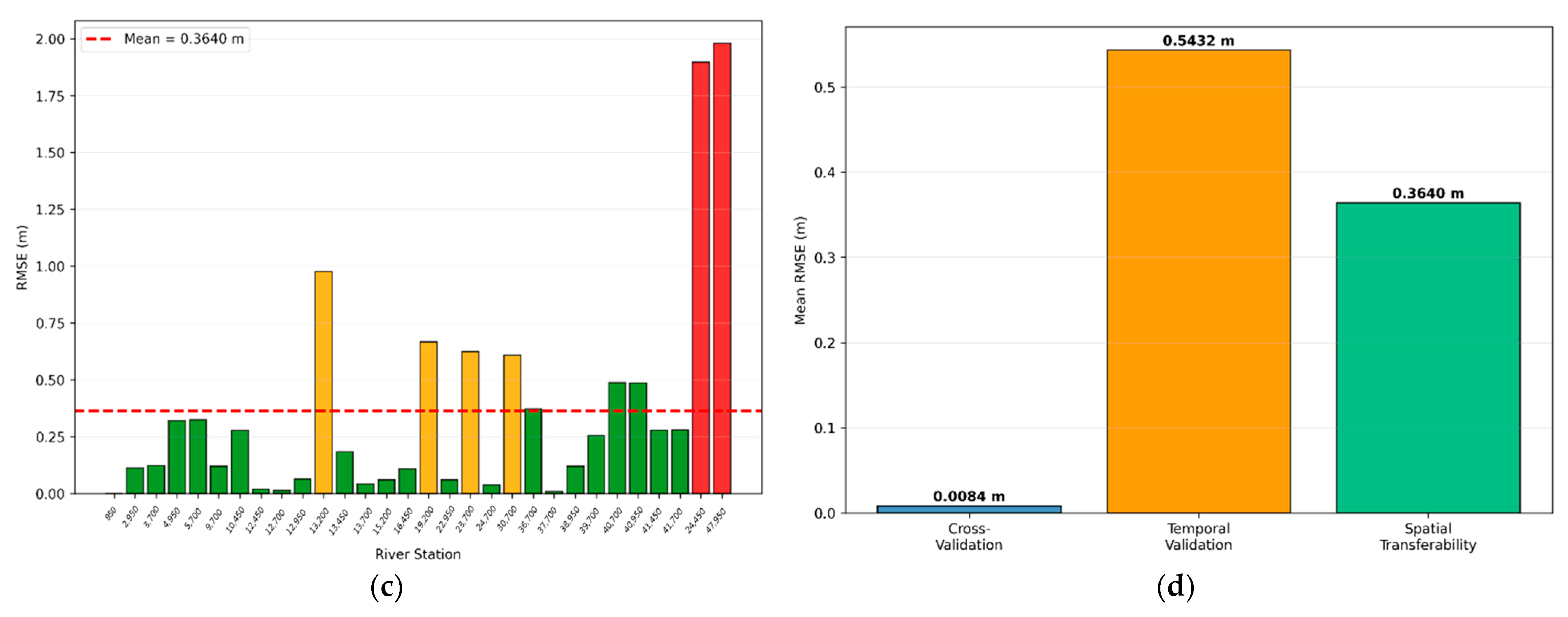
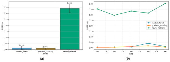
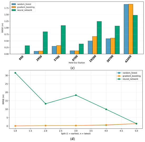
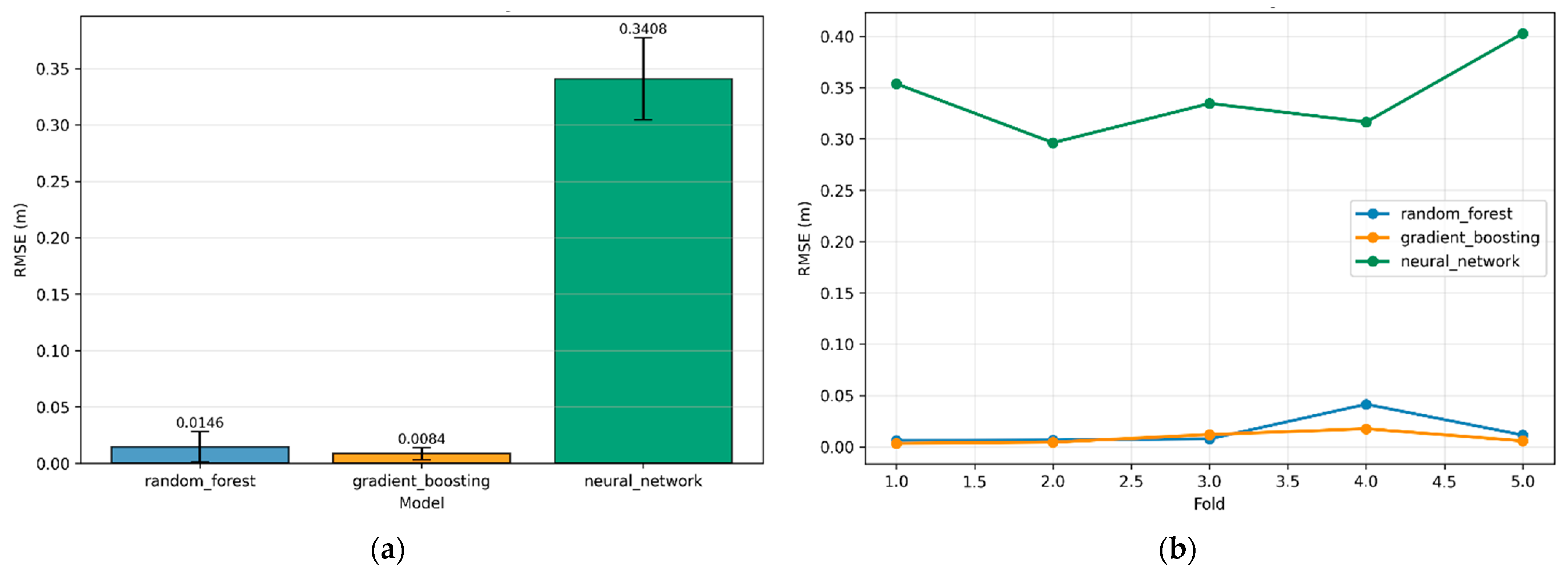
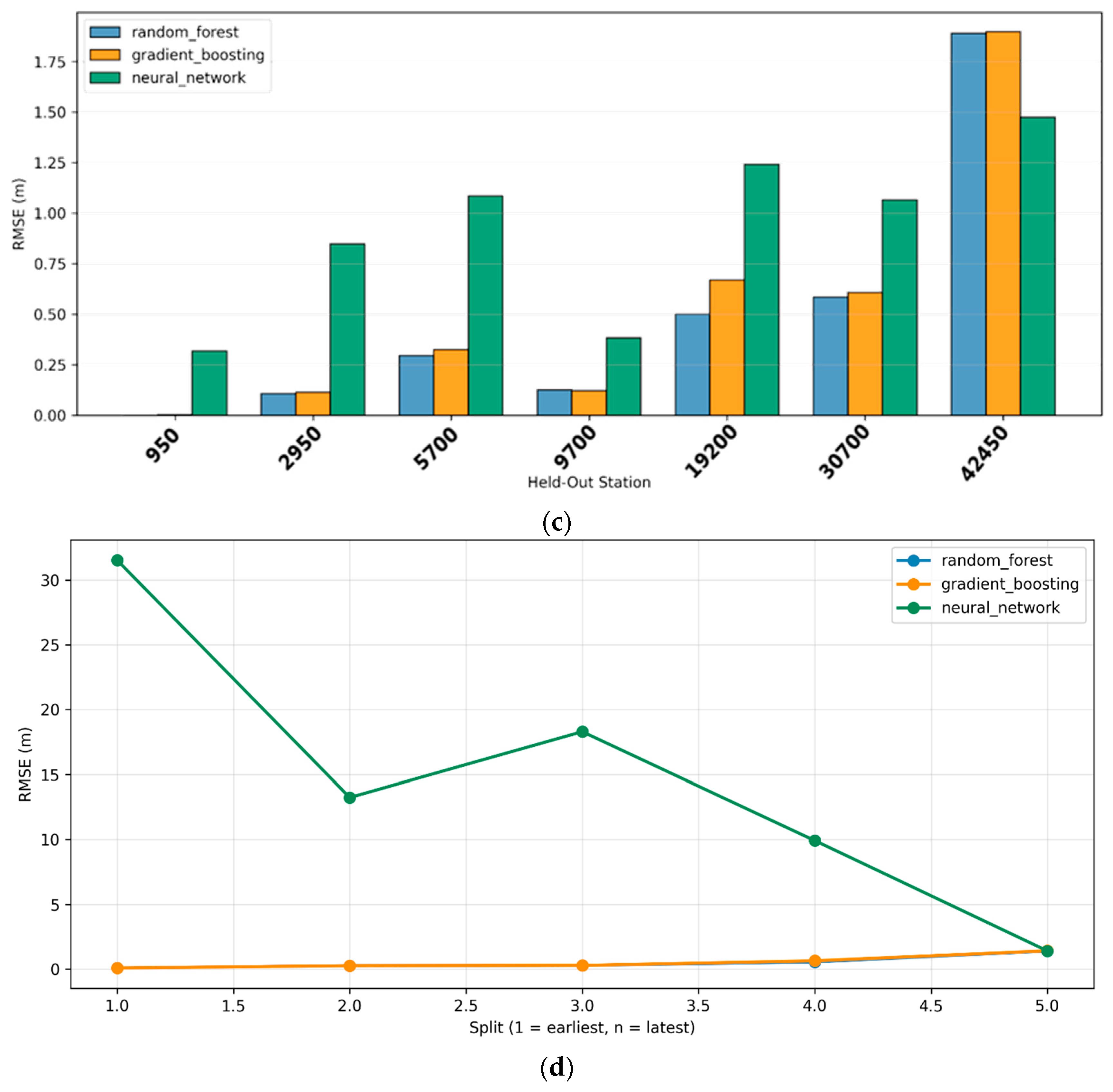

Disclaimer/Publisher’s Note: The statements, opinions and data contained in all publications are solely those of the individual author(s) and contributor(s) and not of MDPI and/or the editor(s). MDPI and/or the editor(s) disclaim responsibility for any injury to people or property resulting from any ideas, methods, instructions or products referred to in the content. |
© 2026 by the authors. Licensee MDPI, Basel, Switzerland. This article is an open access article distributed under the terms and conditions of the Creative Commons Attribution (CC BY) license.