


Abstract
In many developing regions, the lack of on-site weather data impedes the estimation of rainfall-driven processes, such as soil erosion. Satellite-based precipitation products (SPPs) can support hydrological modelling in gauge-sparse regions by providing continuous rainfall estimates. Accurate rainfall estimation is crucial to soil erosion modelling, particularly in data-scarce regions such as the TRB. In this study, seven satellite-based precipitation products—CHIRPS, IMERG, TRMM, ERA5, GLDAS, and PERSIANN-CDR, along with the IMD gridded dataset—were evaluated for their ability to represent rainfall patterns and support R-factor estimation in the RUSLE framework. This is the first comprehensive evaluation of multiple SPPs for RUSLE-based soil erosion modelling in the Tungabhadra river basin (TRB), providing insights for ungauged watersheds in India. CHIRPS and IMERG displayed relatively smooth and continuous patterns, while PERSIANN-CDR and TRMM exhibited fragmented rainfall zones. ERA5 and GLDAS demonstrated consistent but moderate values across the basin. IMD data served as the reference product for comparison. The findings reveal that the choice of precipitation dataset directly affects the accuracy of erosion estimation. Therefore, multi-dataset evaluation is recommended for reliable assessment of soil loss and watershed planning in ungauged or partially gauged catchments.
1. Introduction
In developing countries, hydrological modelling for watershed management, land planning, and soil conservation strategies is often constrained by the lack of dense ground-based hydro-meteorological stations [1,2,3]. However, technological developments in satellite remote sensing have opened up options, which facilitates conducting large-scale environmental studies with reasonable accuracy [4,5,6]. Among the remote sensing data currently available, rainfall information is key for soil erosion studies, especially in semi-arid areas like the Tungabhadra river basin (TRB), which features large-scale agriculture and varied uneven terrain that lead to land degradation [7,8].
Soil erosion causes land degradation, loss of soil fertility, sedimentation in reservoirs, and a general decline in land productivity [9,10,11]. To that end, the Revised Universal Soil Loss Equation (RUSLE) has become widely used to estimate average annual soil loss based on various environmental factors [12,13]. Among its input variables, the rainfall erosivity factor (R) is key to understanding the role of rainfall intensity and kinetic energy in soil detachment and transport. However, there is a lack of reporting from rain gauge stations, and their distribution is uneven, which particularly affects large and remote watersheds [14].
To address this problem, various forms of satellite precipitation products (SPPs) have emerged, providing full spatial coverage, improved temporal frequency, and enhanced spatial accuracy [14]. The study that was conducted by Saravanan et al. [15] serves to assess soil erosion hazards in the Katteri watershed using the USLE and Geographic Information System (GIS) techniques. According to the authors in Saravanan et al. [16], precipitation damages the upper layers of soil structure through the impact of falling raindrops and the shear velocity of flowing water, with higher rainfall intensity accelerating soil erosion. Additionally, changes in land use and land cover influence soil erosion rates, whereas dense vegetation reduces erosion. According to Sathiyamurthi et al. [17], the soil type and topography of a study area remain relatively stable over time; therefore, changes in precipitation and vegetative cover are the key factors determining whether soil erosion rates increase or decrease. The present study focuses specifically on precipitation as the driving factor. In the Wunna watershed, Singh & Saravanan [18] used various precipitation datasets as inputs to ArcSWAT to simulate runoff and then compared the simulated results with observed runoff values from the Central Water Commission (CWC) to identify the dataset that yielded the highest R-squared value. Similarly, in a study by Kaliraj et al. [19], precipitation datasets for the years 2000, 2010, and 2023 were used to generate R-factor maps, and decadal variations in soil erosion rates were identified in the Mannarkad watershed in the Palakkad district, India. Building on these approaches, the present study inputs various precipitation datasets into the RUSLE-GIS model to identify the dataset that best aligns with Indian Meteorological Department (IMD) gridded rainfall data for creating an R-factor map of the TRB. These datasets have been widely used to model erosion processes, but their accuracy and reliability depend on several factors, including region, climatic zone, and physiographic features [20]. Thus, it is essential to assess the adequacy of these datasets for RUSLE in terms of accurately representing rainfall distribution and estimating R-factor values before proceeding [21].
This study evaluates the effectiveness of multiple satellite precipitation datasets, including CHIRPS, TRMM, IMERG, PERSIANN-CDR, ERA5, and GLDAS, along with IMD gridded data, for deriving the R-factor across the TRB. Using Google Earth Engine (GEE), spatial patterns of the R-factor from each dataset were compared to assess their suitability for soil erosion modelling [22,23,24]. The findings support improved understanding and application of satellite data for erosion studies in ungauged or poorly gauged watersheds [25,26].
Using GEE, the spatial rainfall pattern/variation/distribution of each SPP dataset has been arrived at [27]. The outcome supports improved understanding and application of satellite data for erosion studies in ungauged or poorly gauged basins.
2. Study Area and Data Used
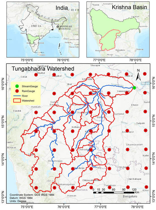
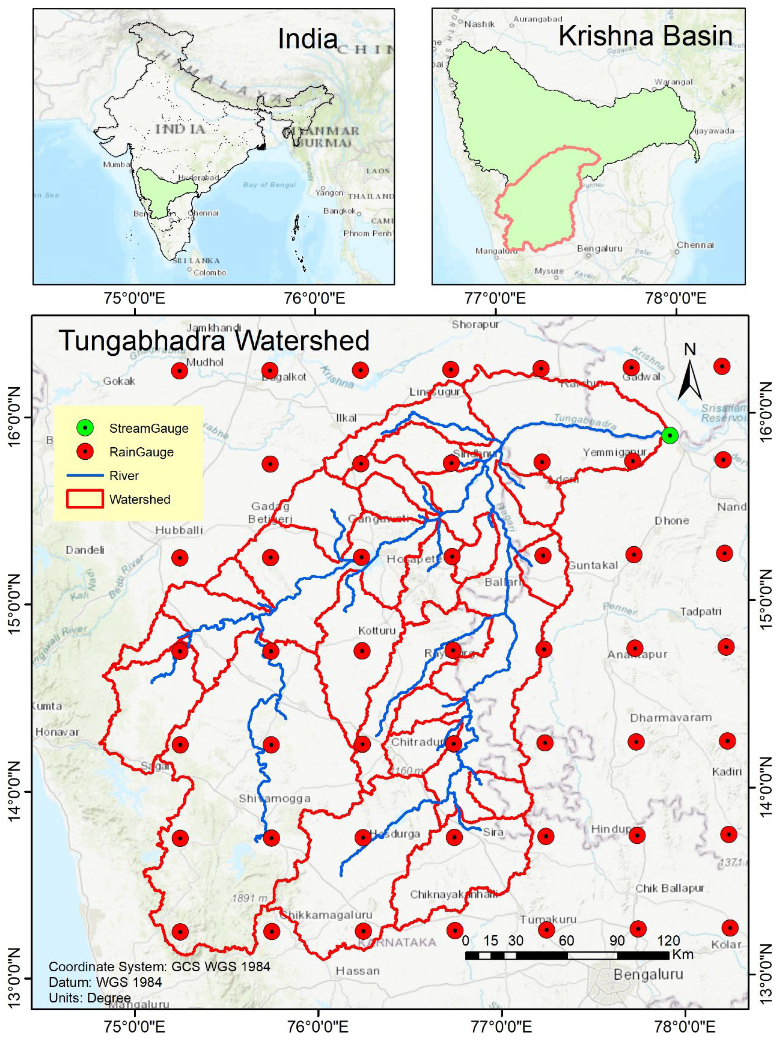
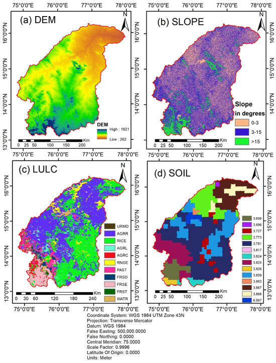
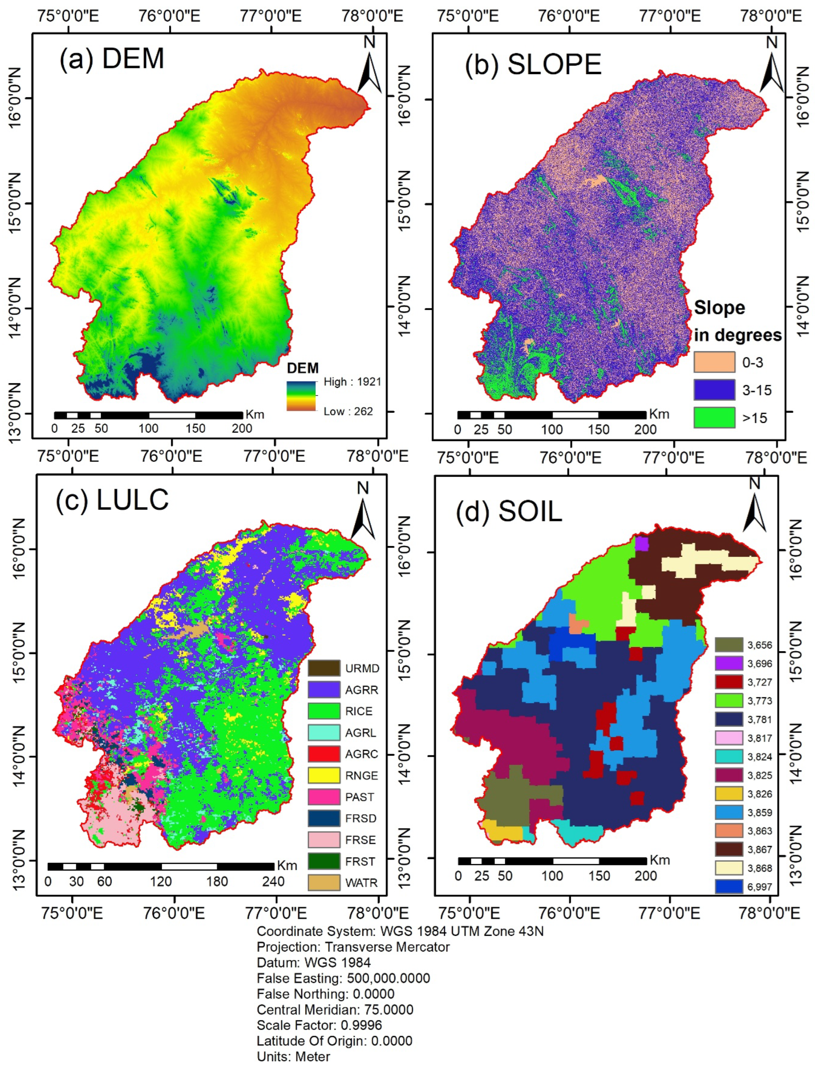
As shown in Figure 1, the TRB, a sub-basin of the Krishna River system, is located in the southern part of India, covering regions of Karnataka, Andhra Pradesh, and Telangana. It originates in the Western Ghats of Karnataka and flows eastward before merging with the Krishna River. The basin is situated between approximately 13°28′ N to 15°36′ N latitudes and 75°07′ E to 77°42′ E longitudes. The terrain is characterised by rugged hills in the west and gradually sloping plains in the east. The basin’s elevation ranges from about 300 m to over 1921 m as taken from the Digital Elevation Model (DEM) shown in Figure 2.
Figure 1.
A map of the TRB showing selected 0.25-degree IMD (CRS: WGS 84-UTM 43N).
Figure 2.
(a) DEM, (b) slope, (c) LULC and (d) soil distribution of Tungabhadra river basin.
2.1. Climate and Hydrogeology of the Region
The TRB experiences a semi-arid to dry sub-humid climate, with monsoonal rainfall patterns. The significant proportion of the rainfall occurs in the period of the south-west monsoon season, while during the remaining period of the year, the region remains relatively dry. Owing to the fact that uneven rainfall distribution is a characteristic feature here compounded by a high dependence on agriculture for livelihood, and intense land use, the basin is facing challenges and continues to remain vulnerable to soil erosion and land degradation.
The basin provides resources to carry on agricultural activities and is equipped with critical water infrastructure, which includes the Tungabhadra reservoir, canals, and command areas. However, reservoir sedimentation due to upstream erosion has become a significant concern for reservoir life and irrigation efficiency.
From a geological viewpoint, the basin is supported upon the crystalline foundation of the Peninsular Gneissic Complex (PGC), which is primarily composed of granite gneisses and granites significantly occupying the western and southern basin sectors [28]. Geomorphologically, the region’s landforms are, by and large, a product of denudational–structural processes and fluvial erosion. The alluvial soil cover within the TRB varies in thickness between 10 and 26 m. The river contributes heavy sediment loads to the Krishna system, which has created the fertile Raichur Doab (lying between the Tungabhadra and Krishna rivers), a region noted for its prominent alluvial plains.
The study area experiences a consistently hot tropical climate, averaging 33 °C annually. As depicted in Table 1, agricultural landscapes cover more than four-fifths of the watershed, featuring a mix of stepped cultivation in hilly regions and irrigated farming in the plains. Farming practices vary from mixed cropping on terraced hills to irrigated plains agriculture, supporting the production of major crops such as sugarcane, groundnut, and paddy.
Table 1.
LULC statistics of the study area.
2.2. Source of Data
The datasets as shown and used for the study were selected based on spatial coverage, resolution, and relevance for RUSLE factor estimation. All the datasets shown in Table 2 were processed using GEE and ArcGIS 10.4.
Table 2.
The datasets used in the study and their sources.
2.3. Preparation of LULC Map
LULC plays a significant role in the RUSLE model by influencing both the cover management factor (C) and the support practice factor (P). In this study, the LULC map as shown in Figure 2 was prepared using Sentinel-2 (10 m) datasets. The images were processed on the GEE platform, and supervised classification was performed to distinguish major land use categories, including cropland, forest, built-up land, water bodies, and barren land.
C-factor was determined with the usage of the NDVI (Normalised Difference Vegetative Index). LULC classes were reclassified based on erosion potential to estimate the P factor. The derived LULC maps were subsequently used for soil erosion modelling. The datasets for the study were selected based on spatial coverage, resolution, and relevance to RUSLE factor estimation.
3. Methodology
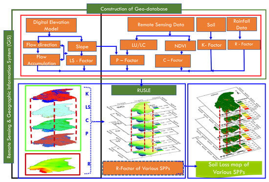
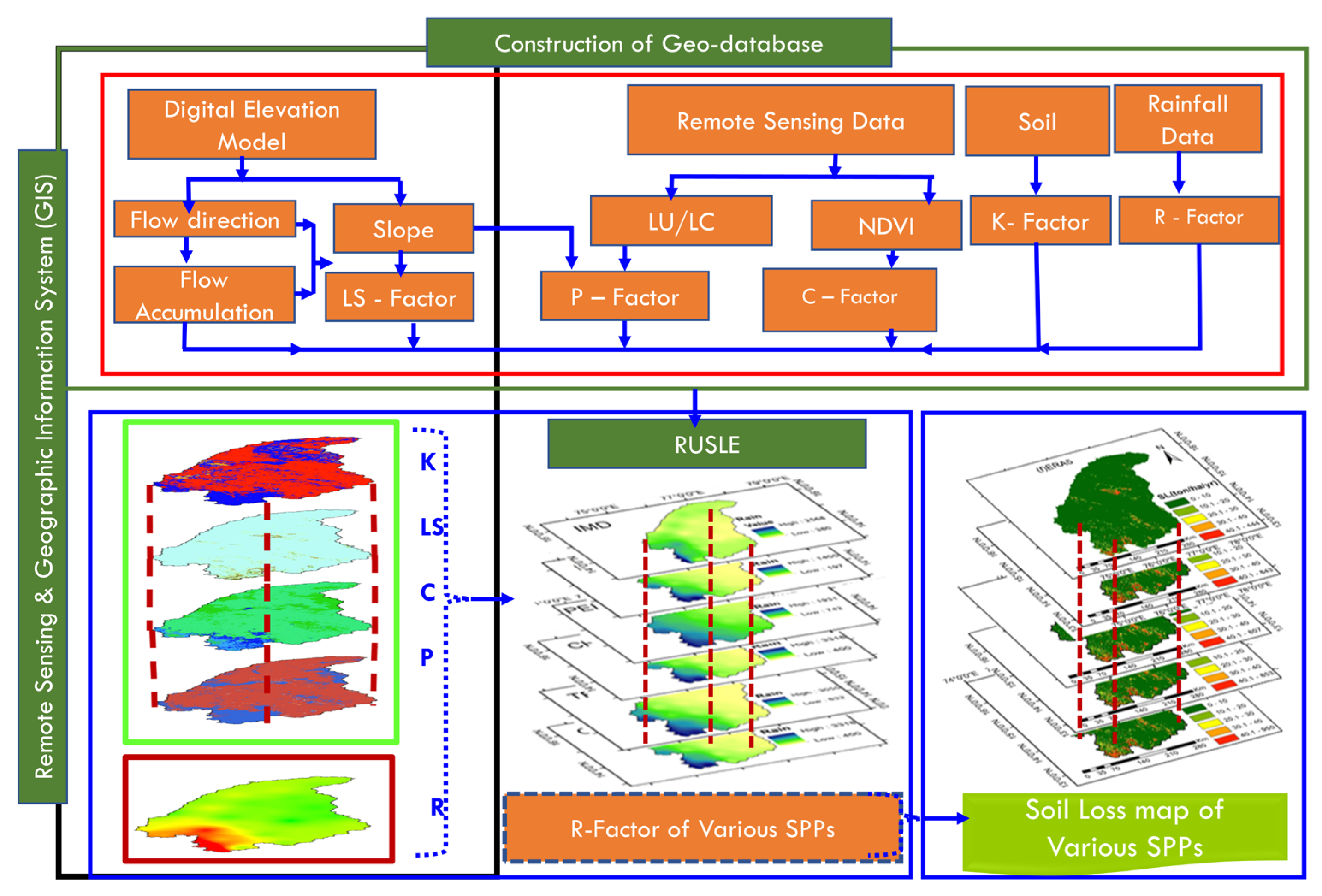
This study incorporated the RUSLE model, supported on a GEE platform and a remote sensing (RS) GIS environment, to provide an estimation of soil loss plus the spatial variation in annual soil loss across the TRB. The RUSLE model computes soil erosion as a quantity dependent upon five important parameters like rainfall erosivity (R), soil erodibility (K), slope length–slope steepness (LS), vegetative cover factor (C), and management/conservation practice (P). These essential factors/products are derived from the combination of satellite datasets, reanalysis precipitation products, and advanced spatial analysis techniques. The entire methodological workflow is depicted in Figure 3.
Figure 3.
Methodology flow chart.
3.1. Satellite-Based and Reanalysis Precipitation Products
In this study, seven satellite-based and reanalysis rainfall datasets shown in Table 3 were utilised to analyse rainfall temporally and find the R-factor for the TRB. The selected datasets include CHIRPS, TRMM, IMERG, GLDAS, ERA5, PERSIANN-CDR, and IMD. These datasets are different in spatial resolution, methodologies for data retrieval, and varying data sources; however, they were selected for their availability across all regions of the globe, consistency, and user-end support on cloud computing platforms like GEE.
Table 3.
Description of the various SPPs and their sources utilised in this study.
CHIRPS combines satellite imagery with ground station observations to deliver precipitation estimates at 0.05° spatial resolution, making it suitable for drought monitoring and soil erosion modelling. TRMM provides 0.25° resolution rainfall estimates derived from microwave and infrared sensors on the TRMM satellite and has been widely used in tropical rainfall research. IMERG, developed under the Global Precipitation Measurement (GPM) mission, improves upon TRMM by offering 0.1° resolution precipitation data corrected using GPCC observations, thereby enhancing performance in detecting light rainfall.
GLDAS offers global precipitation data by integrating satellite and in situ observations through land surface modelling at 0.25° resolution, making it useful for large-scale hydrological studies. ERA5, a global reanalysis product by ECMWF, provides precipitation estimates through advanced data assimilation and modelling systems, suitable for high-resolution rainfall assessment. PERSIANN-CDR uses artificial neural networks applied to satellite infrared data to estimate precipitation, with bias correction using GPCC, and is of 0.25° spatial resolution, offering long-term consistency. Finally, the IMD gridded rainfall dataset provides high-resolution daily precipitation across India based on extensive rain gauge networks and this serves as a reference for validation.
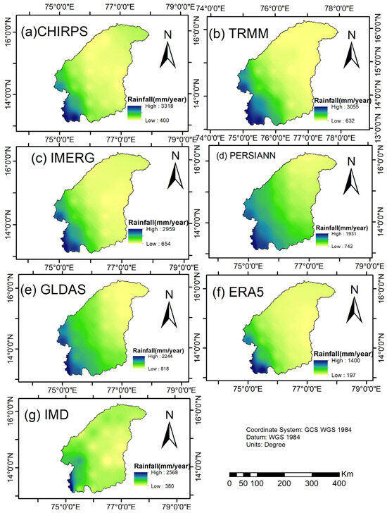
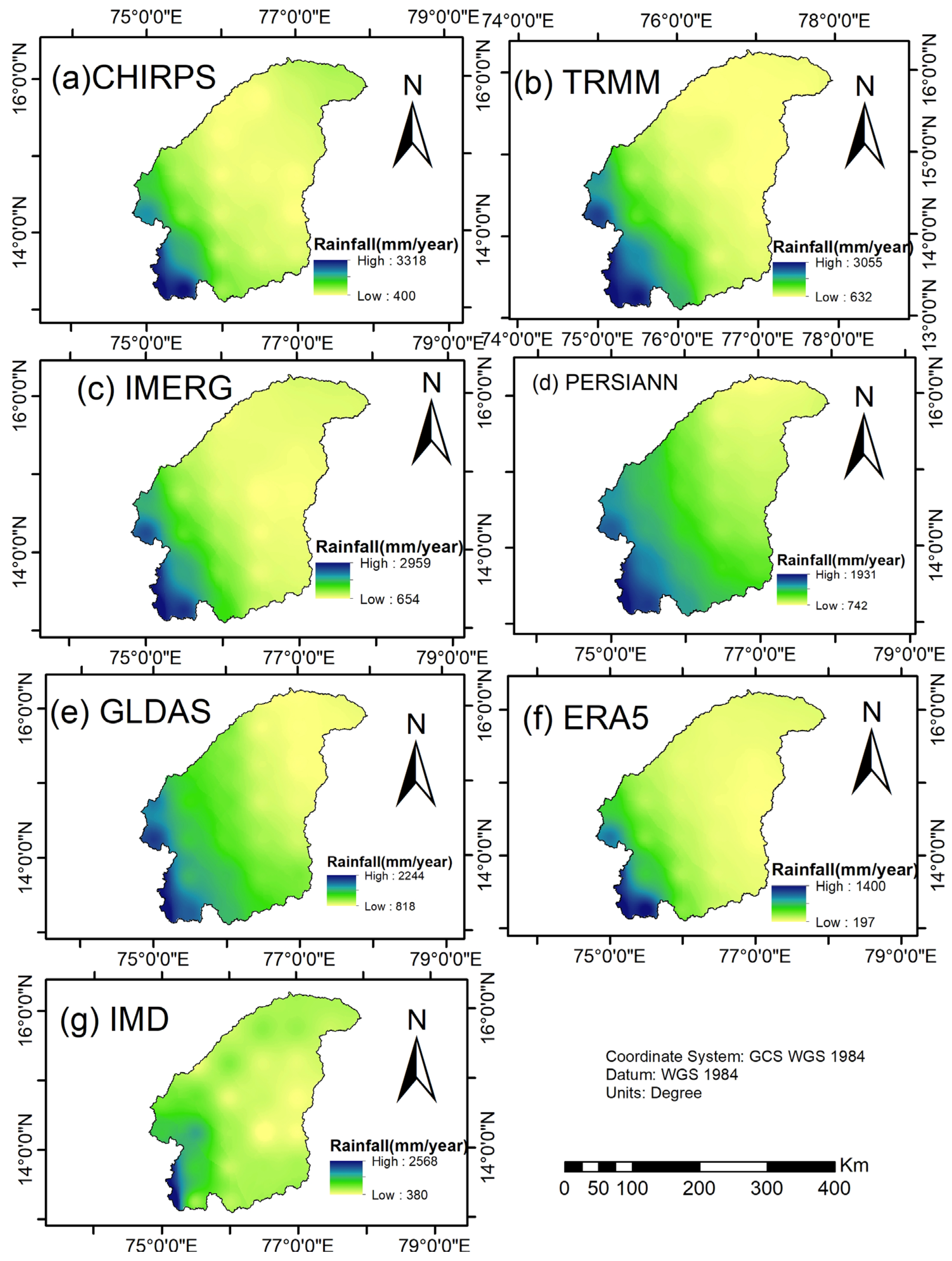
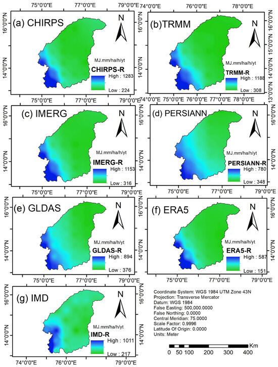
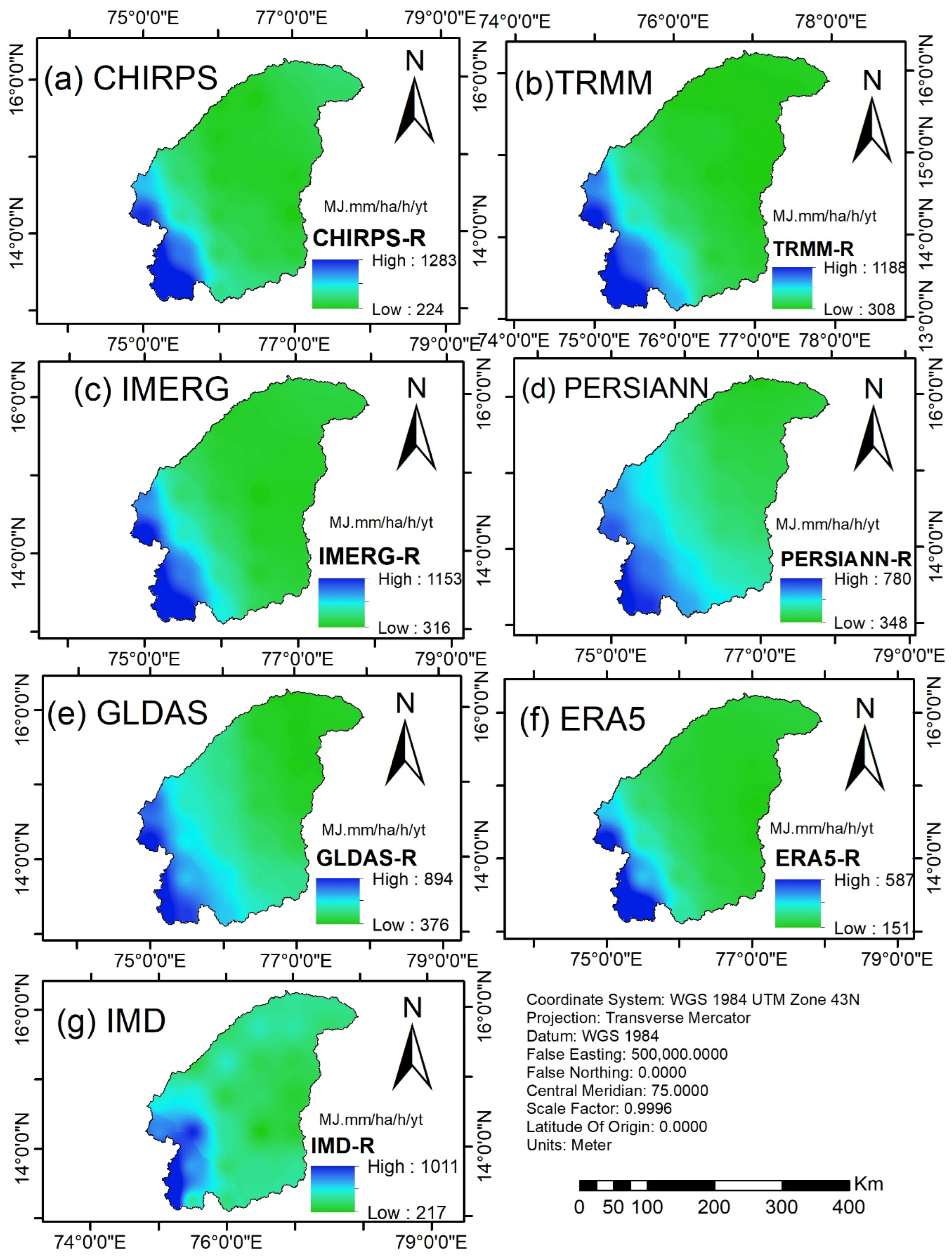
The consideration of these diverse rainfall datasets enabled an overall estimation of the R-factor, ensuring a spatially robust and temporally consistent assessment of rainfall-induced erosion potential across the TRB. Figure 4 shows the spatial variation in average annual rainfall as observed through various sources of datasets over the TRB.
Figure 4.
Spatial distribution of average annual rainfall (mm/year) of (a) CHIRPS (b) TRRM, (c) IMERG, (d) PERSIANN, (e) GLDAS (f) ERA5, (g) IMD map of TRB.
3.2. Integrating the RUSLE Model with GEE Plus RS and GIS
The RUSLE model was implemented in GEE for the estimation of annual soil erosion throughout the TRB.
GEE offers access to diverse satellite datasets and powerful cloud computing, allowing for the integration and processing of large-scale spatial data to calculate RUSLE factors (R, K, LS, C, and P).
The RUSLE model computes annual soil loss (A) using five key factors: R-factor, K-factor, LS-factor, C-factor, and P-factor. In this study, each factor was derived from remote sensing datasets processed in GEE. Soil loss (in ton/ha/yr) is estimated using Equation (1) below.
A = R × K × LS × C × P
In Equation (1), the average annual soil loss per unit area, expressed as ton/hectare/year, is denoted as A. The R-factor, measured in MJ-mm-ha−1-h−1 year−1, is represented by R. The K-factor, given in t-ha−1 MJ−1-mm−1, is indicated by K. LS stands for the slope length and steepness factor. The C-factor is defined as C, while the P-factor is represented by P. LS, C and P are dimensionless. The five factors influencing map creation are detailed below.
The RUSLE-SDR model as per Williams and Berndt [29] computes sediment yield in ton/ha/yr (SY-Equation (2)) at the Bawapuram stream gauge station using two key factors (annual soil loss and sediment delivery ratio (SDR-Equation (3)) using the equations below:
where SLP is the slope in percentage derived from the DEM satellite product.
3.2.1. R-Factor
The R-factor, representing the erosive power of rainfall, was computed using precipitation datasets processed within the GEE platform. For this study, the IMD rainfall datasets were selected due to their high accuracy [30]. Annual precipitation (P, in mm) was calculated and converted into the R-factor using the empirical relationship in Equation (4).
R = 0.363 × P + 79
Equation (2), validated for monsoon-dominated regions in India [30], provides a reliable estimate of rainfall erosivity. Other satellite-based precipitation datasets (CHIRPS, IMERG, TRMM, ERA5, and GLDAS) were used for comparative analysis to assess spatial variability in R-factor estimates.
3.2.2. K-Factor
The K-factor is an important part of the RUSLE model because it shows how easily soil particles can be moved by rain and surface runoff. It mostly depends on the soil’s texture, organic matter content, structure, and permeability. Changes in these properties have a significant influence on soil erosion rates.
For this study, we used high-resolution, globally available soil texture data instead of detailed field-based soil surveys because the TRB covers a large area and has a lot of different types of terrain. The OpenLandMap-Soil Texture USDA-TT (v02) dataset prepared by [31] was used through the GEE platform. This dataset provides reliable information regarding soil texture classes on a global scale that is generated from harmonised soil databases.
To arrive at the K-factor, each unique type of soil texture was allotted a unique erodibility value based on published literature and look-up tables. With the help of conditional expressions coded in the GEE environment, soil textures like sandy, sandy loam, loamy sand and silty clay were quantified into K-factor values. For instance, soils having more silt content are likely to be the most erodible of all soils. They can be easily detached, tend to crust and lead to high rates of runoff. Values of K for these soils are likely to be more than 0.4. The K-factor map shows how different areas of soil are more/less vulnerable to erosion and helps in making later estimates of soil loss [32].
3.2.3. LS-Factor
The LS-factor represents the significance of the topography in the RUSLE model. Slope steepness (S) indicates the steepness of the terrain, which plays a role in how rapidly surface runoff velocity increases, thus increasing the erosive effect of the water. If the steepness increases, water will runoff faster, putting a new shear stress on the soil particles, making them move and detach from each other. Slope length (L) is the distance from the beginning of overland flow to the point where it enters or deposits in a channel. It reveals the region upslope that collects runoff. Longer slopes allow for more water and momentum to flow through, accelerating erosion. The LS factor considers all these factors to demonstrate how the terrain contributes to erosion. This alters the amount of soil that can be lost beyond what the R and K factors would imply. The LS-factor in RUSLE is dimensionless and leads to different estimates of erosion. Higher values mean that the area would erode more quickly, particularly in hilly or mountainous areas.
Geospatial tools, such as GEE/ArcGIS, analyse DEMs to create the LS-factor, enabling watershed-scale analyses to consider more complex flows versus assuming uniform slopes (as defined by the original USLE). The LS-factor was calculated using the flow accumulation strategy in this study. This approach models the convergence of overland flow and is appropriate for large basins characterised by mixed forms of terrain. The LS-factor was calculated using Equation (5):
Flow accumulation is expressed as the amount of upslope cells causing runoff at a given point (using the DEM). Cell size corresponds to the spatial resolution of the DEM (here 30 m (ASTER data)). The standard unit plot length is 22.13 m, and m is an exponent that varies with slope steepness (typically 0.4–0.5 for moderate slopes; e.g., adjusted by rill-to-inter-rill erosion ratios). In soil erosion models, such as RUSLE, LS-factor is an important factor as it directly impacts how much energy and sediment can be washed out of the land. Thus, in areas characterised by high LS, light rain can cause considerable erosion, as concentrated flow erodes channels (rills and gullies) and topsoil, causing nutrient loss, low agricultural productivity, and downstream sedimentation. By contrast, low LS values in flat areas favour deposition rather than erosion.
Studies have shown that LS calculation mistakes, likely resulting from the resolution of the DEM or from flow algorithms, can result in 20–50% errors around total soil loss estimates; thus, high resolution data with validated methods are critical. Because the severity of rainfall is growing as a result of climate change, resulting in an increase in runoff on steep slopes, accurate LS mapping is important for prioritising conservation measures.
In the TRB, the LS-factor map was created using the 30 m ASTER Global DEM processed in GEE, which provided values from 0 (flat plains where there is little flow accumulation) to 60.7 (highland areas where the slope is steep and long). This is in line with typical values in semi-arid Indian watersheds, where LS values can exceed 50 in rugged terrains from lengthy flow paths and gradients ranging from 30 to 40 percent. The highest LS values (20–60) were found in the hilly western areas, e.g., close to the origins of the Tunga and Bhadra rivers (Western Ghats) and in the eastern highland area (Sandur hills). These are elevations over 1000 m, with granite outcrops and ravines. These landscape features facilitate flow convergence and rapid surface runoff.
3.2.4. Cover Management Factor (C-Factor)
C-factor indicates how extensive vegetation coverage, crop residues, and land management practices influence water-borne soil erosion. It is an essential component of the RUSLE model and allows one to see how beneficial ground cover can be to counter the adverse effects of erosive rainfall and surface runoff. Vegetation-rich areas function well in reducing the detachment and erosion of soil particles while areas with reduced or no vegetation are more prone to erosion [33]. This study obtained the C-factor using the NDVI obtained from 10 m resolution Sentinel-2 satellite imagery. The NDVI is a customary measure for healthy and dense vegetation and has known applications in erosion modelling for vegetation cover assessment as per [33]. The NDVI was calculated with Equation (6), using reflectance at the near-infrared (Band 8) and red (Band 4) spectral bands of Sentinel-2.
To convert the NDVI into the C-factor, the method suggested by [33] was followed, which applies an exponential transformation as shown in Equation (7).
The empirical constant α is fixed as 2, which allows a smooth representation of vegetation density. Higher NDVI (vegetation) values correspond to lower C-values while lower NDVI (bare soil) will correspond to higher C-values. The C-factor map was produced where values ranged between 0 and 1, indicating a continuous spread of vegetation cover throughout the study area. This approach offers a more rigorous and realistic estimation of C-values compared to relying only on static categories and has also been performed successfully in earlier soil erosion research [34,35,36].
3.2.5. P-Factor
The P-factor represents the effect of activities on soil conservation and land management techniques like contouring, strip cropping, and terracing in controlling water erosion rates. Because we have no ground-based conservation data for the entire TRB, we chose to use a combined slope–LULC approach to estimate the spatial variability of P-factor values. This approach involved extraction of LULC data from the Sentinel-2 (10 m) dataset and calculating the slope percentages from ASTER 30 m GDEM as per terrain slope function. These slopes were converted into percentages and labelled according to thresholds for agricultural areas, in agreement with [37] and recent GIS erosion studies.
3.3. Model Validation
In this study, the accurate assessment of soil loss due to erosion is performed by adopting a validation approach by Masroor et al. [38]. The sediment yield obtained from the RUSLE-SDR technique with R-factor computed with TRMM data was validated with the sediment data obtained from the Krishna Godavari basin organisation (CWC) from the years between 2006 and 2011. The observed sediment yield at the outlet Bawapuram was 0.7 ton/ha/yr and that obtained in this study through the RUSLE-SDR method using TRMM data was 0.84 ton/ha/yr. The soil erosion map post-2012 was validated with a fractional area water erosion map produced by the National Remote Sensing Centre (NRSC), Indian Space Research Organisation (ISRO), Government of India. Soil erosion values were extracted from the estimated soil erosion map and NRSC fractional soil erosion map [39]. A correlation was established between the estimated soil erosion map and NRSC fractional soil erosion map. Without direct ground-level soil loss measurements throughout the Tungabhadra sub-basin, the aforesaid indirect validation techniques were incorporated. Streamflow data collected from the observed gauging stations and the literature were used through hydrological consistency checks as a proxy to utilise the model outputs for soil erosion. From the precipitation datasets we tested, it was also observed that the IMERG rainfall-based RUSLE model closely matched hydrological variables recorded there and had appropriate spatial coverage of soil loss. The IMERG-based model predicted relatively high soil erosion in these areas, which spatially coincided with regions exhibiting elevated sediment yield and surface runoff. This correspondence suggests that the model is responsive to rainfall-driven hydrological processes and spatial variability; however, the observed agreement should be interpreted as indicative rather than conclusive evidence of model performance. The reproducibility of average soil loss estimates from other datasets (e.g., CHIRPS, TRMM and PERSIANN-CDR) produced consistent results for high erosion areas, and, therefore, our confidence regarding the RUSLE findings based on these rainfall inputs increased. Not directly measuring sediment yield or soil erosion to calibrate the model but spatial erosion trends was in line with some critical landscape parameters—topography, vegetation cover and slope gradients—proving that in such an ungauged catchment as Tungabhadra, the RUSLE model would be relevant and applicable. Overall, the grid points produced were 84 in the study area with a spatial resolution of 0.25° × 0.25°. Soil loss was determined for each grid point from the RUSLE-based soil loss maps produced by different satellite precipitation products (SPPs) like CHIRPS, IMERG, TRMM, ERA5, PERSIANN and GLDAS.
The data extracted are then regarded as alternative estimates (Oi) and the reference values for soil loss of IMD precipitation (Gi) are incorporated as a reference value. Then, the paired datasets at grid locations were used for a comparative statistical performance analysis and ROC-AUC analysis in order to find out the robustness, reliability and discriminative power of SPP-based soil loss estimates against IMD-based soil loss estimates. Differences between IMD-based soil loss estimates (Gi) and other gridded precipitation datasets (Oi) were then compared based on standard error indices such as RMSE (RMSE-Equation (8)), MAE (MAE-Equation (9)), MBE (MBE-Equation (10)), and relative bias (RB-Equation (11)). These metrics include error size, average deviation, systematic bias, and percentage bias, respectively.
The RMSE highlights larger errors and is expressed as:
The MAE represents the average absolute deviation between soil loss computed with gauged observations (Gi) and other SPPs (Oi):
The MBE indicates the direction and magnitude of systematic bias:
Relative bias (RB) expresses the bias as a percentage of IMD gauged soil loss values:
3.4. Receiver Operating Characteristic (ROC) Curve and Area Under the Curve (AUC) Analysis
As per Davis & Goadrich [40], ROC analysis (Table 4 shows confusion matrix) was used to assess how well soil loss estimates from different precipitation datasets distinguish between various erosion levels compared to the IMD reference. The ROC curve depicts the true positive rate (TPR) along the y-axis versus the false positive rate (FPR) along the x-axis, over different soil loss thresholds. The AUC offers a threshold-independent performance measure, ranging from 0.5 (random guessing) to 1.0 (perfect discrimination). Greater AUC values is an indicator of stronger agreement with the reference dataset and better ability of the precipitation data to capture soil loss variability.
Table 4.
Confusion matrix.
AUC is the total area under the ROC curve, where the x-axis is the false positive rate (FPR) and the y-axis is the true positive rate (TPR) as computed from Equation (12) and Equation (13) respectively.
Using the trapezoidal rule for discrete points (xk, yk) on the ROC curve, the AUC is calculated by Equation (14) below.
An MS-Excel document is used for calculating the true positive rate/false positive rate. After input of this excel file, an R program also gives the AUC. This R program is available on request. The sum runs over all threshold points k from 1 to n.
4. Results
4.1. A Study on Geographical Changes in the Components of the RUSLE Model
If considering the spatial variation in RUSLE parameters, it is necessary to look for the behaviour of R, K, LS, C, and P, the parameters, which differ in different locations. This process helps to identify patterns and trends in soil erosion risk within the study area. Usually, remote sensing data along with GIS tools are relied upon to visually analyse these variations, which supports effective soil conservation practices.
4.1.1. R-Factor Map
Figure 5 shows R-factor maps for the TRB, generated by spatially interpolating using the inverse distance weighted method (IDW) to estimate erosivity values at all grid locations within the study area. The R-factor values range from 151 to 1283 MJ-mm/ha/h/yr.
Figure 5.
Spatial distribution R-Factor (in MJ.mm/ha/h/y) map of (a) CHIRPS (b) TRRM (c) IMERG (d) PERSIANN (e) GLDAS (f) ERA5 (g) IMD of TRB.
4.1.2. K-Factor Map
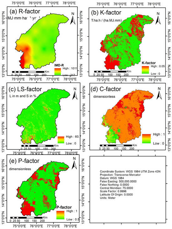
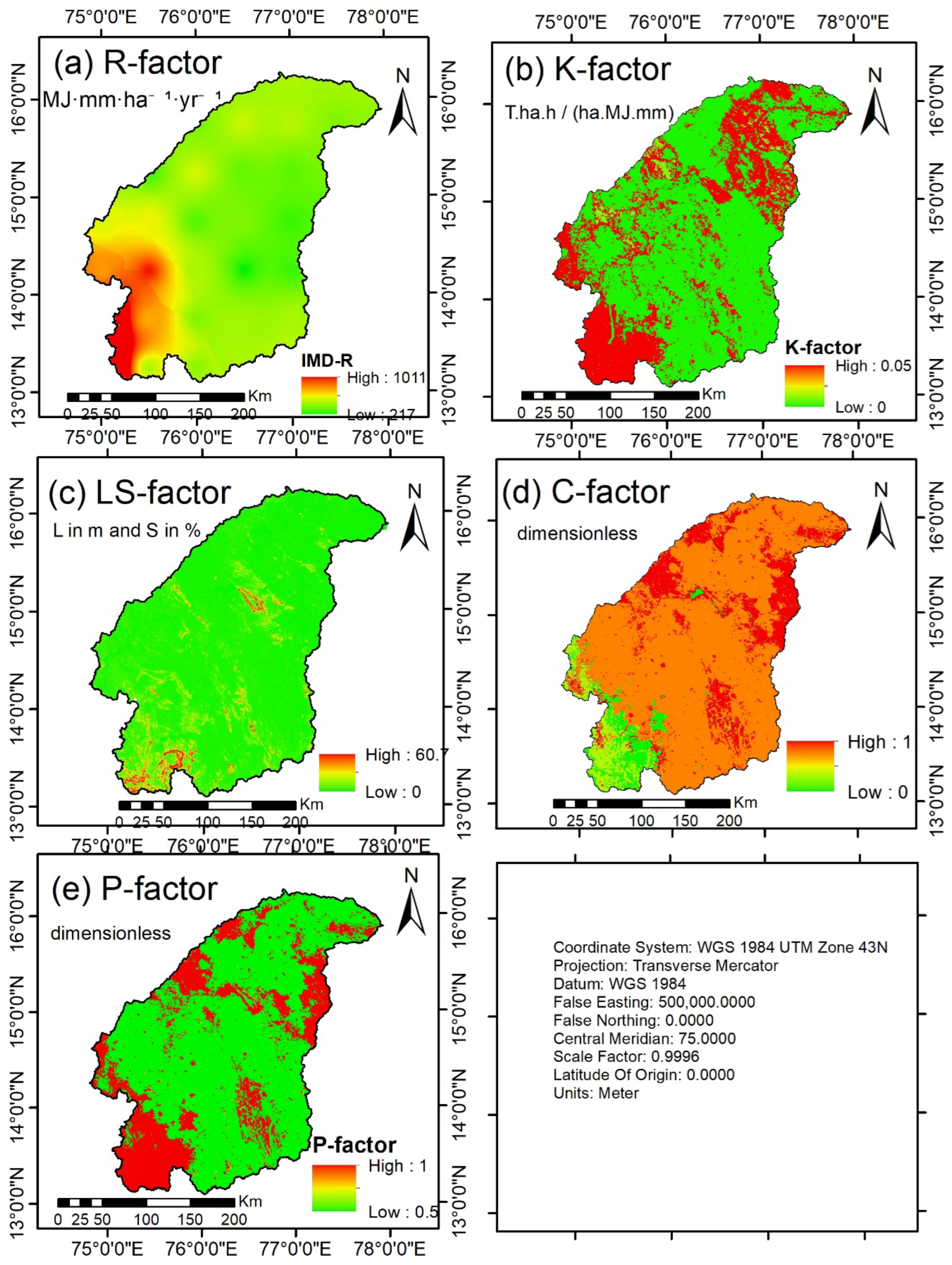
In the RUSLE model, K-factor is determined through characteristics like soil texture [40] As illustrated in Figure 6b, a map derived from the SOILGRIDS250m dataset shows K-factor values across the TRB ranging from 0.0264 to 0.05 t/ha/h/ha/MJ/mm. These areas of heightened erodibility are more prone to intense soil erosion.
Figure 6.
(a–e): Various RUSLE factor maps of the TRB (a) R-factor(IMD) (b) K-factor (c) LS factor (d) C-factor (e) P-Factor.
4.1.3. LS-Factor Map
Slope steepness (S) indicates the rate at which or how sharply the surfaces of the slopes rise/fall, while slope length (L) describes the flow length. Thus “L” and “S” are the most essential properties of the soil erosion model, and combined LS represents the topographical component of the map.
The generated LS-factor map shows values that fall in the range of 0 to 60.6784. Maximum LS-factor values appear in hilly and high-elevation zones, while the lowest are mainly in flat areas (the eastern side of the TRB) with gentle slopes. The sharply rising/falling slopes can be found in the western as well as eastern highland regions of the sub-basin, making them increasingly prone to soil erosion. The spatial variation is illustrated in Figure 6c.
4.1.4. C-Factor Map
The NDVI-derived C-factor map (Figure 6d) demonstrates pronounced spatial variability in vegetation-mediated erosion control. Forested zones with high NDVI values yield minimal C-factor values particularly in certain south-western areas of the TRB, reflecting effective surface protection. Agricultural landscapes exhibit moderate C-factor values driven by heterogeneous crop cover conditions. Bare land exhibits the highest C-factor values, indicating elevated erosion susceptibility, while water bodies such as the Tungabhadra reservoir display negligible values as they are not exposed to soil erosion processes.
4.1.5. P-Factor Map
With reference to Table 4 and the P-factor (shown in Figure 6e), a representation of the impact of support practices on soil erosion is mapped with values from 0 to 1. The assignment considers slope, land use type, and cultivation methods—particularly irrigation and conservation measures—as referenced in Table 5. Higher P-values indicate areas with fewer conservation interventions, where soil is more readily transported downhill and deposited in lower regions.
Table 5.
Values of P-factor for various LULC categories obtained from the published literature by [41].
4.2. Compression Assessment of Annual Soil Erosion Using RUSLE for Various SSP
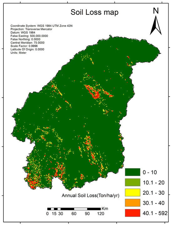
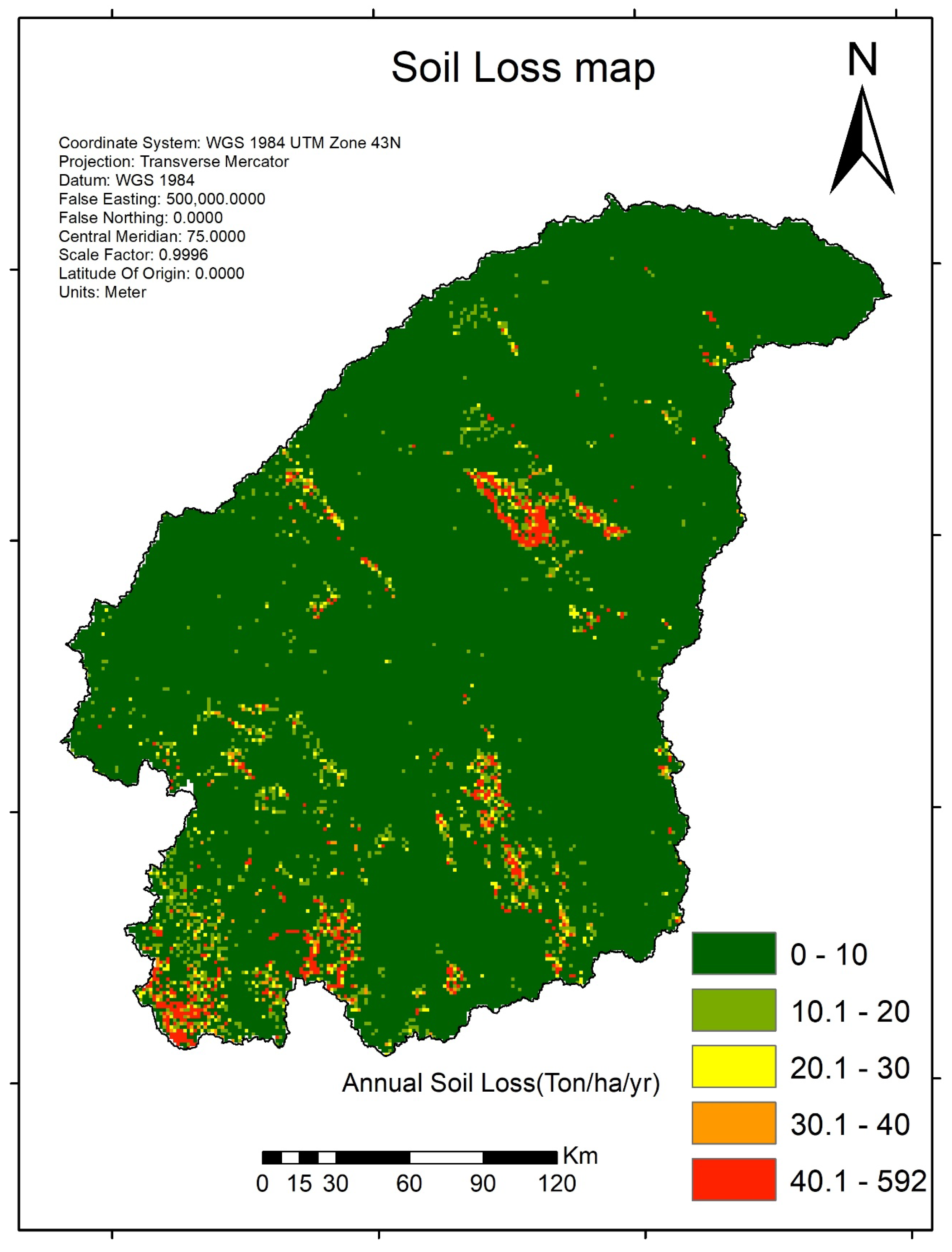
Analysis of the TRB revealed a significant expansion of areas classified under “Very low” soil erosion during the study period. Notably, 5% of the basin’s area has been identified as being at very high risk, and is estimated to be the primary source of soil loss, accounting for most of the basin’s total erosion. The annual soil erosion using IMD data is shown in Figure 7.
Figure 7.
An annual soil loss map (IMD)of the TRB.
To pinpoint high-risk zones in the TRB, specific sub-basins were designated as soil erosion risk areas. These zones experienced soil loss increases of over 20 t/ha/yr. This study finds that seven out of 23 sub-basins showed an annual soil erosion of 20 ton/ha/year or higher. In these sub-watersheds, zones with potential soil loss surpassing 60 ton/ha/year were mainly located in the south-western and central regions of the basin.
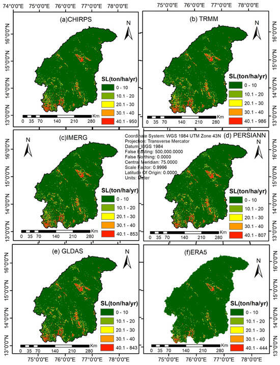
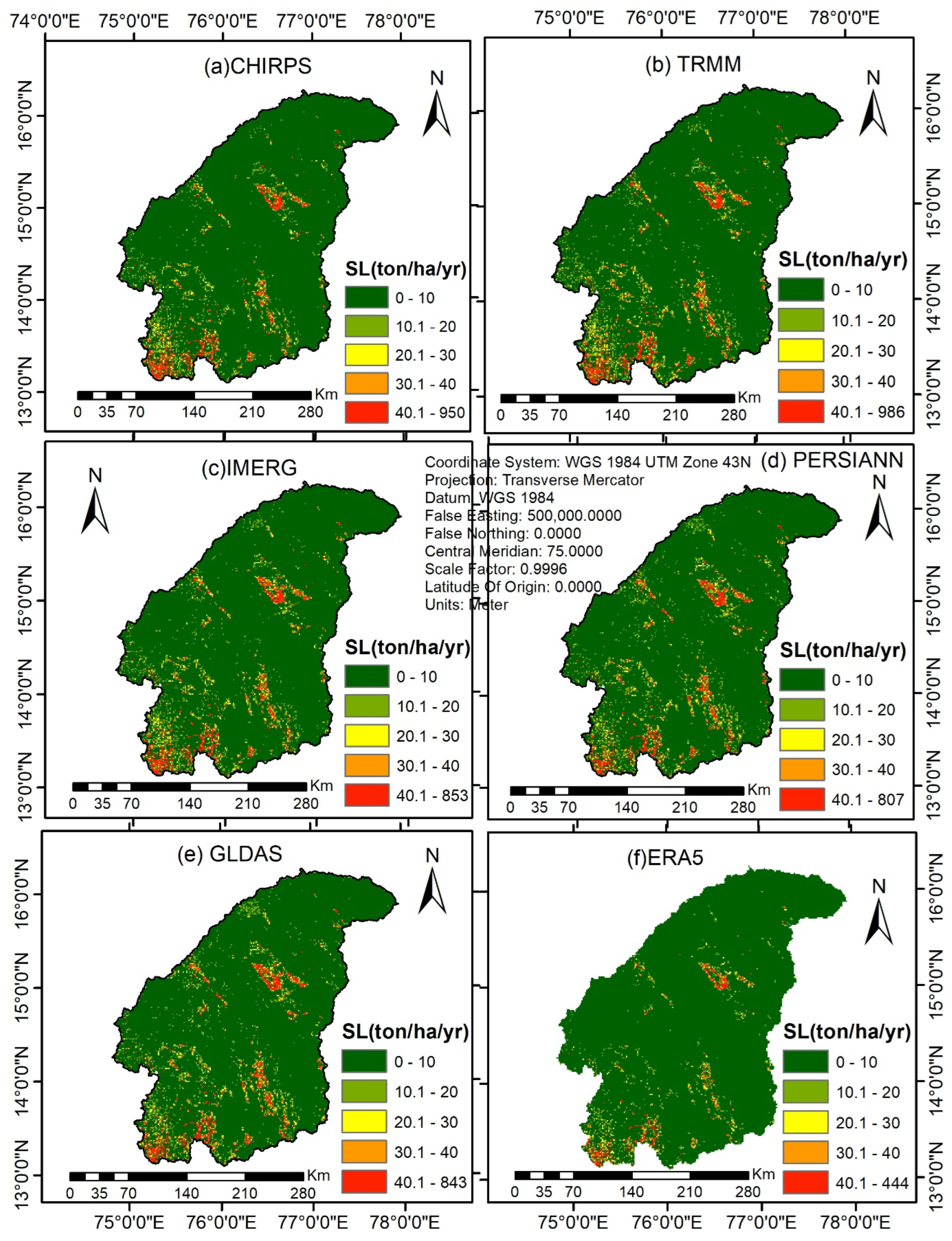
The spatial distribution of annual soil erosion was calculated by overlaying the five factors of the RUSLE model as shown in Figure 8. According to the analysis, the R-factor in the basin ranges from 217 to 1011 MJ mm ha−1 h−1 yr−1.
Figure 8.
The spatial distribution of annual soil erosion (SL)of various SPPS like (a) CHIRPS (b) TRMM (c) IMERG (d) PERSIANN (e) GLDAS (f) ERA5 in the TRB.
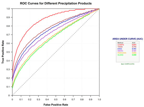
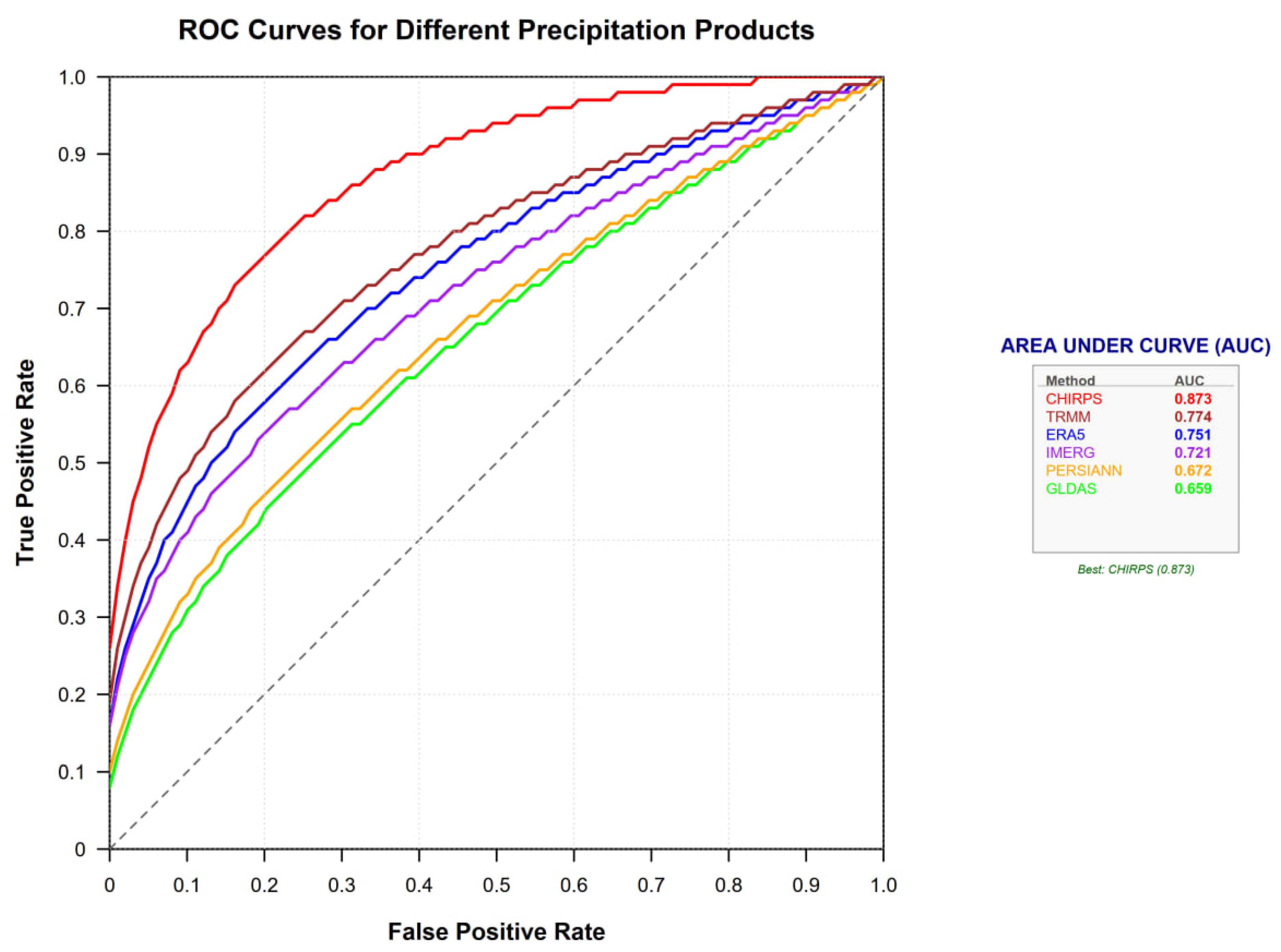
The efficacy of various gridded precipitation datasets in estimating soil erosion via the RUSLE model was assessed through ROC-AUC analysis and standard statistical metrics, using IMD-derived soil loss (S1) as the benchmark. The ROC curves (Figure 9) depict the correlation between the true positive rate (TPR) and the false positive rate (FPR) for soil loss forecasts obtained from the CHIRPS, IMERG, TRMM, ERA5, PERSIANN, and GLDAS datasets.
Figure 9.
ROC curves of varied rainfall datasets.
The ROC analysis indicates significant disparities among the datasets. CHIRPS (S2) achieves the highest AUC value (0.8725), revealing an impressive discriminatory ability and close conformity to the soil loss determined through IMD. Next comes IMERG (S3) (AUC of 0.8599), indicating a strong predictive ability. TRMM (S4) shows moderate performance (AUC = 0.7744), while ERA5 (S5) and PERSIANN (S6) have comparatively lower accuracy with AUC = 0.7206 and 0.7090, respectively. GLDAS (S7) has the lowest AUC (0.6722) which indicates low correlation of the results with the reference dataset. Overall, the ROC results suggest a performance hierarchy of CHIRPS > IMERG > TRMM > ERA5 > PERSIANN > GLDAS.
Table 5 statistical metrics corroborate these ROC findings. The lowest RMSE at CHIRPS (4.598) and MAE (1.05) show little or no variation from the IMD estimates. The error magnitudes increase progressively for IMERG and TRMM, while those with much higher RMSE values (greater than 12) can be seen in PERSIANN and GLDAS. Bias analysis reveals that ERA5 underestimates it significantly (RB = −35.3%) while PERSIANN and GLDAS overestimate it remarkably (greater than 49%). Furthermore, mean annual soil loss rates between datasets differ, highlighting the importance of differences in the precipitation inputs for RUSLE outputs.
5. Discussion
5.1. Effect of R-Factor on Soil Loss
The TRB is an important agricultural region in southern India. The last few decades have seen marked changes in rainfall and LULC patterns owing to climatic variability and greater anthropogenic activities. These changes have affected both the spatial diversity and strength of the R-factor, an essential factor influencing erosion of soil, derived mainly from the RUSLE model. To investigate how these changes would affect the rate of erosion of the soil, the current research tried looking at fluctuations of the R-factor to understand the long-term environmental trend in the basin. Selected years coincide with the available years for satellite-based precipitation data, particularly from PERSIANN-CDR and IMD, and correlate with reported increases in monsoon rainfall intensity [42].
The R-factor quantifies the erosive power of rainfall and was computed using the empirical formula in Equation (4) [43,44]. To analyse its spatial variation across 23 sub-basins, the Thiessen polygon method was applied. This geostatistical technique weights rainfall data from weather grid points based on their distance to sub-basin centres, providing an accurate representation of rainfall erosivity across the basin’s diverse terrain. Based on data from PERSIANN-CDR and IMD, R-factor has values that range between 217 and 1011 MJ mm ha−1 h−1 yr−1, reflecting the basin’s exposure to intense monsoon rainfall. These findings align with the literature reports for Indian basins, which report similar ranges for monsoon-dominated regions [29]. The data from IMERG and CHIRPS yielded reliable R-factor values (200–1200 MJ mm ha−1 h−1 yr−1). Conversely, TRMM and PERSIANN-CDR tended to overestimate erosivity in some sub-basins, which could lead to an overestimation of soil loss by 15–20% [45,46].
Overall, the combined ROC-AUC and statistical evaluation demonstrates that CHIRPS and IMERG precipitation datasets provide more reliable soil loss estimates, whereas GLDAS and PERSIANN introduce greater uncertainty in erosion modelling. Table 6 provides a comparative statistical summary of soil erosion estimates using RMSE, MBE, and MAE. Statistical comparisons between soil erosion estimates derived from IMD rain gauges (S1) and six gridded precipitation products—CHIRPS (S2), IMERG (S3), TRMM (S4), ERA5 (S5), PERSIANN (S6), and GLDAS (S7)—are performed using IMD rain gauge-based estimates (S1) as the primary reference for comparison. After removing a negligible number of outliers, statistical evaluation indicates that the CHIRPS dataset (S2) agrees most closely with the IMD gauge benchmark (S1), as evidenced by the lowest RMSE (4.60) and MAE (1.05). This highlights the role of data resolution. In contrast, GLDAS (S7) shows the largest deviations (RMSE = 13.86). Bias analysis reveals that most gridded products tend to overestimate, while ERA5 (S4) exhibits a marked underestimation (MBE = −2.43, RB = −35.3%)—a result consistent with the existing literature [47]. These patterns are reflected in the average erosion values in Table 5. Overall, despite an underestimation range of 24–38%, all evaluated products (S2–S7) demonstrate acceptable correlation with the ground-based scenario (S1). Table 6 indicates the values of statistical metrics to compare other precipitation datasets with IMD rain gauge data. These metrics correlate to the datasets used in [43].
Table 6.
Summary of statistical metrics.
The key findings of the study as per Table 6 are:
- IMD (S1) serves as the reference dataset as per Saicharan & Rangaswamy [48] and Bhattacharyya et al. [49]: The mean soil loss estimated using IMD rainfall data was 6.86 t ha−1 yr−1. All statistical metrics for the other datasets are evaluated relative to this benchmark.
- CHIRPS shows the closest agreement with IMD as per Gupta et al. [50]: CHIRPS produced a mean soil loss of 7.31 t ha−1 yr−1, only 0.45 t ha−1 yr−1 higher than IMD. It exhibited the lowest RMSE (4.598 t ha−1 yr−1) and lowest MAE (1.05 t ha−1 yr−1) among all alternative datasets. The relatively low bias (RB = 10.126%) indicates that CHIRPS provides the most comparable soil erosion estimates to the IMD-based model.
- IMERG and TRMM moderately overestimate soil loss as per Emerson [51]. IMERG and TRMM estimated mean soil losses of 7.64 and 7.73 t ha−1 yr−1, respectively. Their positive MBE and RB values indicate systematic overestimation relative to IMD. The RMSE values of 7.776 (IMERG) and 7.909 t ha−1 yr−1 (TRMM) suggest moderate deviations from the reference scenario.
- ERA5 is the only dataset that underestimates soil loss as per Sakhraoui et al. [48]. ERA5 estimated a mean soil loss of 6.30 t ha−1 yr−1, which is lower than the IMD estimate. The negative MBE (−2.429 t ha−1 yr−1) and RB (−35.30%) indicate a consistent underestimation tendency. This suggests that ERA5 may not adequately capture rainfall intensities associated with erosion processes in the basin.
- PERSIANN and GLDAS show the largest deviations. PERSIANN and GLDAS generated the highest mean soil loss estimates (7.79 and 7.86 t ha−1 yr−1, respectively). They exhibited the largest RMSE values (12.433 and 13.857 t ha−1 yr−1) and the highest relative biases (49.47% and 55.71%). These results indicate substantial divergence from the IMD-based estimates and a tendency to considerably overestimate erosion rates.
- Ranking of datasets based on agreement with IMD: Based on RMSE and MAE values, the datasets can be ranked as CHIRPS > IMERG ≈ TRMM > ERA5 > PERSIANN > GLDAS, where CHIRPS shows the strongest agreement, with IMD and GLDAS the weakest.
Since CHIRPS is ranked next to IMD, it can be used for hydrological studies in command areas like in [52].
The overall interpretation of Table 6 is that the statistical comparison indicates that soil erosion estimates are highly sensitive to the choice of precipitation dataset. Among the evaluated products, CHIRPS demonstrated the closest correspondence with the IMD-based reference scenario, whereas PERSIANN and GLDAS exhibited substantial positive biases and larger prediction errors. IMERG and TRMM produced intermediate results with moderate overestimation, while ERA5 consistently underestimated soil loss. These findings suggest that CHIRPS may provide a more suitable alternative rainfall input for RUSLE-based soil erosion assessments in the study area, although the observed agreement should be interpreted as indicative rather than definitive evidence of superior performance.
5.2. Soil Loss Severity Analysis
Soil loss severity classes—very low: <10 t ha−1 yr−1; low: 10–20 t ha−1 yr−1; moderate: 20–30 t ha−1 yr−1; high: 30–40 t ha−1 yr−1; and very high: >40 t ha−1 yr−1—were mapped for the study period based on RUSLE model outputs. The percentage of area covered by each severity class was calculated for each sub-basin, and changes over time were assessed. The results showed a considerable increase in the “severe” soil loss class, especially in seven of the 23 sub-basins identified as erosion hotspots. These hotspots, mainly in the north-western and central regions, experienced soil loss rates exceeding 60 t ha−1 yr−1, due to high R-factor values, steep slopes, and LULC changes. The spatial distribution of soil loss severity was illustrated in Figure 7, emphasising areas critical to watershed management [43].
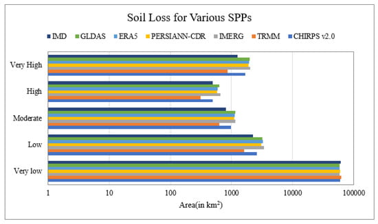
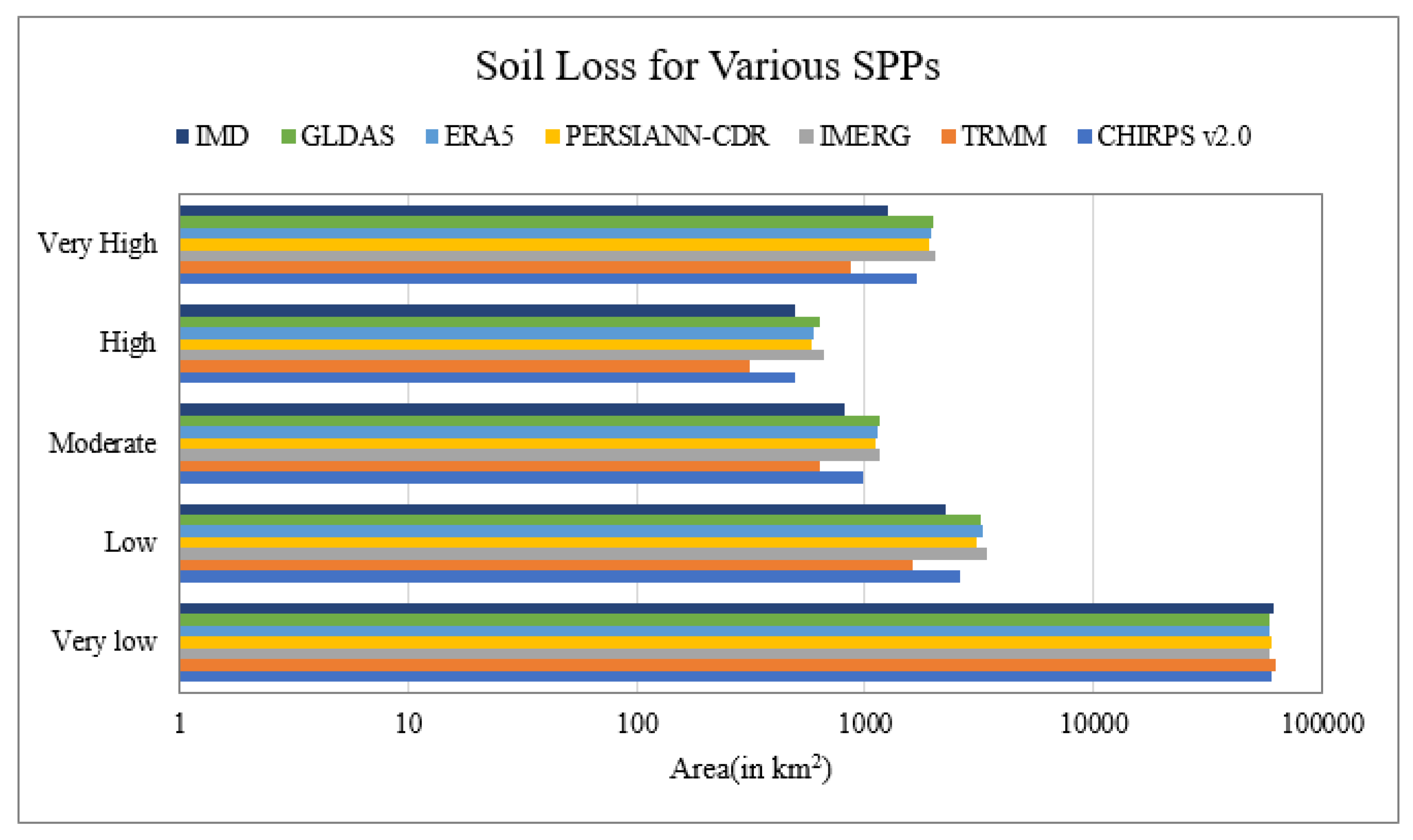
The IMD gridded dataset, serving as a reference, provides a benchmark for the validation of Soil Loss Prevention Products (SPPs). Soil losses derived from R-factor maps created using various SPPs are compared with those obtained from the R-factor map generated based on IMD data, as illustrated in Figure 10 and Table 7 below. Nonetheless, its limited spatial coverage highlights the significance of satellite-based products such as IMERG and CHIRPS, particularly for ungauged catchments. To validate the outputs of the RUSLE model, it is advisable to utilise ground-based soil loss measurements to comprehend the evolving relationship between climate-induced rainfall erosivity and soil erosion over time.
Figure 10.
The area of soil erosion distribution for the seven SSPs in the TRB.
Table 7.
Areal coverage (in km2) under various soil risk categories for various SPPs.
5.3. Implications for Watershed Management
Sub-basins that exhibit substantial increases in R-factor and expansion of cropland are prioritised for the implementation of erosion control strategies, such as contour ploughing, terracing, and reforestation. Areas identified as erosion hotspots, particularly in the north-western and central regions, require focused interventions to mitigate sediment yield, which can have adverse effects on reservoir capacity and water quality as per [32]. These findings underscore the importance of utilising satellite data and spatial analysis in watershed management to address the synergistic impacts of climate change and changes in land use on soil erosion.
The R-factor map, developed using ArcGIS, provided a summary of the average R-factor values for each sub-basin and SPP, revealing a range between 300 and 1200 MJ mm ha−1 h−1 yr−1, which corresponds with the typical values observed in Indian monsoon-driven basins [29]. IMERG and CHIRPS produced the most reliable estimates, closely aligning with data from the India Meteorological Department, whereas TRMM and PERSIANN-CDR occasionally resulted in overestimations of erosivity due to irregular spatial patterns [42].
6. Limitations of the Study
While the RUSLE model integrated with GIS is widely accepted for estimating long-term average annual soil loss values in ton/ha/year at hillslope scale, its application at regional scale with readily available inputs like interpolated rainfall from coarse resolution GEE datasets for calculating R factor, soil grids at 250 m resolution transformed to 30 m K factor datasets by the IDW technique of spatial interpolation, 30 m ASTER GDEM for calculating LS factor, and Sentinel 2A-derived NDVI product for calculating C-factor have introduced several sources of uncertainty in the RUSLE model when applied to the Tungabhadra river basin which is the current area of interest. Also, the uncertainty is compounded by spatial smoothing of LS factor due to medium DEM resolution of 30 m; mixed-pixel effects in C factor from 30 m land cover product obtained from Sentinel 2A satellite imagery; interpolation errors in R and K factors between observation points, thus reducing the weather extremes that largely govern erosive power of rainfall when high, and marginalising local clay patches respectively; and the model’s underlying assumption that erosion is more dependent upon sediment transport rather than sediment detachment. To conclude, the results shall be interpreted as finding relative erosion risk rather than absolute soil loss values. A sensitivity analysis (not performed here for factors other than R factor) would be required to attribute uncertainty to individual factors and this is the limitation of this study. Generally in many studies, P factor is 1 everywhere in the study area when conservation practices are nil, like in [53,54]. However, in this study an attempt has been made to calculate P factor scientifically as per the referenced table mentioned in Table 5.
7. Conclusions
This study illustrates the effectiveness of high-resolution satellite precipitation products (SPPs) and land use/land cover (LULC) data in mapping soil erosion within the TRB. The analysis substantiates that rainfall erosivity (R-factor), influenced by climatic patterns, is a principal factor contributing to soil loss. The significant findings are as follows: (1) Annual rainfall erosivity exhibited considerable variation among data sources, with CHIRPS recording the highest maximum (1283 MJ mm/ha/h/year) and ERA5-Land the lowest (151 MJ mm/ha/h/year). (2) All assessed SPPs underestimated soil erosion when compared to IMD gauge data, with biases ranging from −3.24% (CHIRPS) to −9.3% (IMERG). (3) CHIRPS and TRMM data yielded the most reliable and precise erosion estimates, thus presenting a feasible solution for areas with limited data. (4) The mean annual soil erosion was estimated to be between 6.29 and 7.86 tons per hectare per year across various scenarios. (5) A substantial portion of the basin (90–95%) experiences low to moderate levels of erosion severity. (6) These erosion patterns, particularly in susceptible soils and steep terrains, pose a threat to agricultural productivity and water resource infrastructure due to sedimentation. (7) Elevated RMSE values for GLDAS and PERSIANN-CDR suggest that these datasets necessitate further calibration. Sediment yield was also calculated as per William and Brendt [29] and found to be 0.84 ton/ha/yr. Collectively, these findings lay a critical groundwork for implementing conservation strategies, such as reforestation and sustainable agricultural practices, aimed at mitigating land degradation and preserving basin ecosystems.
8. Future Research Directions
Future research should include ground-based measurements of soil loss to verify RUSLE outputs, since relying solely on streamflow-based validation has drawbacks, such as indirect correlation with sediment yield. Projections of climate change indicating increased rainfall intensity in the TRB could worsen erosivity and soil loss (Van der Knijf [33]). Utilising advanced modelling techniques like machine learning and SWAT models to evaluate future climate and LULC scenarios can support the development of adaptive mitigation strategies. Furthermore, assessing the socioeconomic impacts of erosion, such as losses in agricultural productivity, can inform policies for sustainable land management.
Author Contributions
S.S.: Supervision, methodology, conceptualisation, project administration; R.S.: methodology, conceptualisation, formal analysis, writing—original draft. All authors have read and agreed to the published version of the manuscript.
Funding
This research received no external funding.
Data Availability Statement
The data presented in this study are available on request.
Conflicts of Interest
The authors declare no conflicts of interest.
References
- Joe, P.; Baklanov, A.; Grimmond, S.; Bouchet, V.; Molina, L.T.; Schluenzen, K.H.; Mills, G.; Tan, J.; Golding, B.; Masson, V.; et al. Guidance on integrated urban hydro-meteorological, climate and environmental services: Challenges and the way forward. In Urban Climate Science for Planning Healthy Cities; Springer International Publishing: Cham, Switzerland, 2022; pp. 311–338. [Google Scholar] [CrossRef]
- Bedada, B.A. Comparative rainfall-runoff hydrological modeling over central Ethiopia using ground observation and global satellite precipitation products: Remote sensing support for water resource management. Discov. Appl. Sci. 2025, 7, 826. [Google Scholar] [CrossRef] [Scilit]
- Hader, P.R.P.; Horta, I.T.L.G.; da Silva do Valle, V.A.; Irigaray, C. Hydro-Meteorological Landslide Inventory for Sustainable Urban Management in a Coastal Region of Brazil. Sustainability 2025, 17, 7487. [Google Scholar] [CrossRef] [Scilit]
- Lu, Y.; Wang, L. The current status, potential and challenges of remote sensing for large-scale mangrove studies. Int. J. Remote Sens. 2022, 43, 6824–6855. [Google Scholar] [CrossRef] [Scilit]
- Chen, J.; Chen, S.; Fu, R.; Li, D.; Jiang, H.; Wang, C.; Peng, Y.; Jia, K.; Hicks, B.J. Remote sensing big data for water environment monitoring: Current status, challenges, and future prospects. Earth’s Future 2022, 10, e2021EF002289. [Google Scholar] [CrossRef] [Scilit]
- Sigopi, M.; Shoko, C.; Dube, T. Advancements in remote sensing technologies for accurate monitoring and management of surface water resources in Africa: An overview, limitations, and future directions. Geocarto Int. 2024, 39, 2347935. [Google Scholar] [CrossRef] [Scilit]
- Abdelsamie, E.A.; Abdellatif, M.A.; Hassan, F.O.; El Baroudy, A.A.; Mohamed, E.S.; Kucher, D.E.; Shokr, M.S. Integration of RUSLE model, remote sensing and GIS techniques for assessing soil erosion hazards in arid zones. Agriculture 2022, 13, 35. [Google Scholar] [CrossRef] [Scilit]
- Ejaz, N.; Elhag, M.; Bahrawi, J.; Zhang, L.; Gabriel, H.F.; Rahman, K.U. Soil erosion modelling and accumulation using RUSLE and remote sensing techniques: Case study Wadi Baysh, Kingdom of Saudi Arabia. Sustainability 2023, 15, 3218. [Google Scholar] [CrossRef] [Scilit]
- Rashmi, I.; Karthika, K.S.; Roy, T.; Shinoji, K.C.; Kumawat, A.; Kala, S.; Pal, R. Soil Erosion and sediments: A source of contamination and impact on agriculture productivity. In Agrochemicals in Soil and Environment: Impacts and Remediation; Springer: Singapore, 2022; pp. 313–345. [Google Scholar] [CrossRef] [Scilit]
- Weeraratna, S. Factors causing land degradation. In Understanding Land Degradation: An Overview; Springer International Publishing: Cham, Switzerland, 2022; pp. 5–22. [Google Scholar] [CrossRef] [Scilit]
- Ekka, P.; Patra, S.; Upreti, M.; Kumar, G.; Kumar, A.; Saikia, P. Land degradation and its impacts on biodiversity and ecosystem services. In Land and Environmental Management Through Forestry; Wiley: Hoboken, NJ, USA, 2023; pp. 77–101. [Google Scholar] [CrossRef] [Scilit]
- Luvai, A.; Obiero, J.; Omuto, C. Soil loss assessment using the revised universal soil loss equation (RUSLE) model. Appl. Environ. Soil Sci. 2022, 2022, 2122554. [Google Scholar] [CrossRef] [Scilit]
- Naqvi, S.A.A.; Tariq, A.; Shahzad, M.; Khalid, S.; Tariq, Z.; Salma, U.; Haseeb, M.; Soufan, W. Predicting soil erosion risk using the revised universal soil loss equation (RUSLE) model and geo-spatial methods. Hydrol. Process. 2024, 38, e15248. [Google Scholar] [CrossRef] [Scilit]
- Tran, T.N.D.; Nguyen, B.Q.; Zhang, R.; Aryal, A.; Grodzka-Łukaszewska, M.; Sinicyn, G.; Lakshmi, V. Quantification of gridded precipitation products for the streamflow simulation on the Mekong River basin using rainfall assessment framework: A case study for the Srepok River subbasin, Central Highland Vietnam. Remote Sens. 2023, 15, 1030. [Google Scholar] [CrossRef] [Scilit]
- Saravanan, S.; Sathiyamurthi, S.; Elayaraja, D. Soil erosion mapping of Katteri watershed using universal soil loss equation and geographic information system. J. Indian Soc. Soil Sci. 2010, 58, 418–421. [Google Scholar]
- Saravanan, S.; Jennifer, J.J.; Singh, L.; Thiyagarajan, S.; Sankaralingam, S. Impact of land-use change on soil erosion in the Coonoor Watershed, Nilgiris Mountain Range, Tamil Nadu, India. Arab. J. Geosci. 2021, 14, 407. [Google Scholar] [CrossRef] [Scilit]
- Sathiyamurthi, S.; Ramya, M.; Saravanan, S.; Subramani, T. Estimation of soil erosion for a semi-urban watershed in Tamil Nadu, India using RUSLE and geospatial techniques. Urban Clim. 2023, 48, 101424. [Google Scholar] [CrossRef] [Scilit]
- Singh, L.; Saravanan, S. Evaluation of various spatial rainfall datasets for streamflow simulation using SWAT model of Wunna basin, India. Int. J. River Basin Manag. 2022, 20, 389–398. [Google Scholar] [CrossRef] [Scilit]
- Kaliraj, S.; Abishek, S.R.; Preethy, P.S.; Manokaran, S.; Srinivas, R.; Saravanan, S. Unveiling decadal variability of soil erosion and sediment yield using GIS-based RUSLE and SDR techniques–a case study of mountain watershed of the Western Ghats, India. Environ. Earth Sci. 2026, 85, 38. [Google Scholar] [CrossRef] [Scilit]
- Andualem, T.G.; Hewa, G.A.; Myers, B.R.; Peters, S.; Boland, J. Erosion and sediment transport modeling: A systematic review. Land 2023, 12, 1396. [Google Scholar] [CrossRef] [Scilit]
- Brychta, J.; Podhrázská, J.; Šťastná, M. Review of methods of spatio-temporal evaluation of rainfall erosivity and their correct application. Catena 2022, 217, 106454. [Google Scholar] [CrossRef] [Scilit]
- Kumar, R.; Deshmukh, B.; Kumar, A. Using GEE and GIS for basin scale soil erosion risk assessment: A case study of Chambal River basin, central India. J. Earth Syst. Sci. 2022, 131, 228. [Google Scholar] [CrossRef] [Scilit]
- Jodhani, K.H.; Patel, D.; Madhavan, N.; Singh, S.K. Soil erosion assessment by RUSLE, GEE, and geospatial techniques over Rel river watershed, Gujarat, India. Water Conserv. Sci. Eng. 2023, 8, 49. [Google Scholar] [CrossRef] [Scilit]
- Fahd, S.; Waqas, M.; Zafar, Z.; Soufan, W.; Almutairi, K.F.; Tariq, A. Integration of RUSLE model with remotely sensed data over GEE to evaluate soil erosion in Central Indus Basin. Earth Surf. Process. Landf. 2025, 50, e70019. [Google Scholar] [CrossRef] [Scilit]
- Idowu, D.; Peter, B.G.; Boakye, J.; Cohen, S.; Carter, E. Evaluating Earth observation products for Catchment-Scale operational flood monitoring and risk management in a sparsely gauged to ungauged river basin in Nigeria. Int. J. Appl. Earth Obs. Geoinf. 2025, 138, 104445. [Google Scholar] [CrossRef] [Scilit]
- de Brito, C.S.; da Silva, R.M.; Santos, C.A.G.; Brasil Neto, R.M.; Coelho, V.H.R. Long-term basin-scale comparison of two high-resolution satellite-based remote sensing datasets for assessing rainfall and erosivity in a basin in the Brazilian semiarid region. Theor. Appl. Climatol. 2022, 147, 1049–1064. [Google Scholar] [CrossRef] [Scilit]
- Singh, L.; Saravanan, S. Adaptation of satellite-based precipitation product to study runoff and sediment of Indian River watersheds. Arab. J. Geosci. 2022, 15, 326. [Google Scholar] [CrossRef] [Scilit]
- Appanna, B. An Analysis of Land Resources Planning and Development in Tungabhadra River Basin of Kurnool district, Andhra Pradesh by using Geospatial Technologies. IOSR J. Eng. 2022, 12, 30–34. [Google Scholar]
- Williams, J.R.; Berndt, H.D. Sediment yield prediction based on watershed hydrology. Trans. ASAE 1977, 20, 1100–1104. [Google Scholar] [CrossRef] [Scilit]
- Kolli, R.; Pandey, A.C.; Minakshi, T.; Tiwari, B. Assessment of rainfall erosivity for soil erosion modeling using satellite precipitation products in India. Sci. Total Environ. 2021, 768, 144525. [Google Scholar]
- Hengl, T.; Mendes de Jesus, J.; Heuvelink, G.B.; Ruiperez Gonzalez, M.; Kilibarda, M.; Blagotić, A.; Shangguan, W.; Wright, M.N.; Bauer-Marschallinger, B.; Guevara, M.A.; et al. SoilGrids250m: Global gridded soil information based on machine learning. PLoS ONE 2017, 12, e0169748. [Google Scholar] [CrossRef] [Scilit]
- Renard, K.G.; Ferreira, V.A. RUSLE model description and database sensitivity. J. Environ. Qual. 1993, 22, 458–466. [Google Scholar] [CrossRef] [Scilit]
- Van der Knijf, J.M.; Jones, R.J.A.; Montanarella, L. Soil Erosion Risk Assessment in Europe; EUR 19044 EN; Office for Official Publications of the European Communities: Luxembourg, 2000; p. 34. [Google Scholar]
- Pandey, A.; Mathur, A.; Mishra, S.K.; Mal, B.C. Soil erosion modeling of a Himalayan watershed using RS and GIS. Environ. Earth Sci. 2009, 59, 399–410. [Google Scholar] [CrossRef] [Scilit]
- Panagos, P.; Borrelli, P.; Meusburger, K.; Alewell, C.; Lugato, E.; Montanarella, L. Estimating the soil erosion cover-management factor at the European scale. Land Use Policy 2015, 48, 38–50. [Google Scholar] [CrossRef] [Scilit]
- Koirala, P.; Thakuri, S.; Joshi, S.; Chauhan, R. Estimation of soil erosion in Nepal using a RUSLE modeling and geospatial tool. Geosciences 2019, 9, 147. [Google Scholar] [CrossRef] [Scilit]
- Wischmeier, W.H.; Smith, D.D. Predicting Rainfall Erosion Losses: A Guide to Conservation Planning; Handbook No. 537; US Department of Agriculture, Science and Education Administration: Washington, DC, USA, 1978. [Google Scholar]
- Masroor, M.; Sajjad, H.; Rehman, S.; Singh, R.; Rahaman, M.H.; Sahana, M.; Avtar, R. Analysing the relationship between drought and soil erosion using vegetation health index and RUSLE models in Godavari middle sub-basin, India. Geosci. Front. 2022, 13, 101312. [Google Scholar] [CrossRef] [Scilit]
- NRSC. Indian Land Degradation Data set 2005-6. NICES/DS(L)/LD/2006/Jan2016. Available online: https://bhuvan-app3.nrsc.gov.in/data/download/index.php (accessed on 8 May 2026).
- Davis, J.; Goadrich, M. The relationship between Precision-Recall and ROC curves. In Proceedings of the 23rd International Conference on Machine Learning, Seoul, Republic of Korea, 6–11 June 2026; pp. 233–240. [Google Scholar] [CrossRef] [Scilit]
- Farhan, Y.; Nawaiseh, S. Spatial assessment of soil erosion risk using RUSLE and GIS techniques. Environ. Earth Sci. 2015, 74, 4649–4669. [Google Scholar] [CrossRef] [Scilit]
- Setti, M.V.; Van Westen, C.J.; Eriksson, L.M. Soil erosion risk prediction using a RUSLE and GIS-based approach in the Cauvery Basin, India. Environ. Earth Sci. 2018, 77, 524. [Google Scholar]
- Yaswanth, K.; Kona, M.; Andra, S.K.; Rathinasamy, M. Understanding the impact of changes in land-use land-cover and rainfall patterns on soil erosion rates using the RUSLE model and GIS techniques: A study on the Nagavali River basin. J. Water Clim. Change 2022, 13, 2648–2670. [Google Scholar] [CrossRef] [Scilit]
- Ekka, A.C.; Mishra, P.K.; Panda, S.N.; Kalbar, P.P.; Jha, M.K. Reservoir storage and utilization in the Cauvery River Basin, India: Current status and future challenges. Water Resour. Manag. 2022, 36, 2391–2410. [Google Scholar]
- Fenta, A.A.; Yasuda, H.; Haregeweyn, N.; Belay, A.S.; Hadush, Z.; Gebremedhin, M.A.; Mekonnen, G. Validation of CHIRPS satellite rainfall estimates over Lake Tana Basin, Ethiopia. Atmos. Res. 2018, 221, 213–225. [Google Scholar] [CrossRef] [Scilit]
- Polong, F.; Deng, K.; Pham, Q.B.; Linh, N.T.T.; Abba, S.I.; Ahmed, A.N.; El-Shafie, A. Separation and attribution of impacts of changes in land use and climate on hydrological processes. Theor. Appl. Climatol. 2023, 151, 1337–1353. [Google Scholar] [CrossRef] [Scilit]
- Sakhraoui, F.; Abu Arra, A.; Şişman, E. Assessing reanalysis ERA-5 LAND precipitation data for soil erosion modeling: Performance, challenges, and insights. Earth Sci. Inform. 2025, 18, 450. [Google Scholar] [CrossRef] [Scilit]
- Saicharan, V.; Rangaswamy, S.H. A comparison and ranking study of monthly average rainfall datasets with IMD gridded data in India. Sustainability 2023, 15, 5758. [Google Scholar] [CrossRef] [Scilit]
- Bhattacharyya, S.; Sreekesh, S.; King, A. Characteristics of extreme rainfall in different gridded datasets over India during 1983–2015. Atmos. Res. 2022, 267, 105930. [Google Scholar] [CrossRef] [Scilit]
- Gupta, V.; Jain, M.K.; Singh, P.K.; Singh, V. An assessment of global satellite-based precipitation datasets in capturing precipitation extremes: A comparison with observed precipitation dataset in India. Int. J. Climatol. 2020, 40, 3667–3688. [Google Scholar] [CrossRef] [Scilit]
- Emberson, R.A. Dynamic rainfall erosivity estimates derived from IMERG data. Hydrol. Earth Syst. Sci. 2023, 27, 3547–3563. [Google Scholar] [CrossRef] [Scilit]
- Sankriti, R.; Subbarayan, S. Irrigation water balance spatio temporal modelling using GEE and GIS in NSLBC command area South India. Discov. Sustain. 2026, 7, 769. [Google Scholar] [CrossRef] [Scilit]
- Demirci, A.; Karaburun, A. Estimation of soil erosion using RUSLE in a GIS framework: A case study in the Buyukcekmece Lake watershed, northwest Turkey. Environ. Earth Sci. 2012, 66, 903–913. [Google Scholar] [CrossRef] [Scilit]
- Chen, T.; Niu, R.Q.; Li, P.X.; Zhang, L.P.; Du, B. Regional soil erosion risk mapping using RUSLE, GIS, and remote sensing: A case study in Miyun Watershed, North China. Environ. Earth Sci. 2011, 63, 533–541. [Google Scholar] [CrossRef] [Scilit]

Disclaimer/Publisher’s Note: The statements, opinions and data contained in all publications are solely those of the individual author(s) and contributor(s) and not of MDPI and/or the editor(s). MDPI and/or the editor(s) disclaim responsibility for any injury to people or property resulting from any ideas, methods, instructions or products referred to in the content. |
© 2026 by the authors. Licensee MDPI, Basel, Switzerland. This article is an open access article distributed under the terms and conditions of the Creative Commons Attribution (CC BY) license.