


Abstract
Reference evapotranspiration (ET0) is a standardized climatic index of atmospheric evaporative demand defined and calculated within the FAO-56 Penman–Monteith (PM) framework. When the required quality-controlled meteorological inputs are available, the standardized FAO-56 PM formulation remains the appropriate method for calculating ET0. This study does not seek to replace that formulation. Instead, it presents a preliminary, site-specific comparative investigation of how six machine learning architectures emulate an existing FAO-56 PM-derived ET0 target. Linear Regression (LR), Random Forest (RF), Extreme Gradient Boosting (XGBoost), Support Vector Regression (SVR), Multilayer Perceptron (MLP), and Long Short-Term Memory (LSTM) were evaluated using 1827 daily records from ERA5-Land/Open-Meteo for Western Macedonia, Greece. The evaluation combined chronological data partitioning, time-series-aware cross-validation, hydrological performance metrics, Diebold–Mariano comparisons, and SHAP-based interpretation. Radiation- and temperature-related variables were the strongest statistical predictors. SVR achieved the lowest test-set RMSE (0.0862 mm day−1; R2 = 0.9967; PBIAS = 0.96%), although its predictive accuracy was not statistically distinguishable from XGBoost (DM = −1.8884, p = 0.0600). LSTM achieved substantially lower accuracy (R2 = 0.7636) under the present experimental configuration. These findings characterize the comparative statistical performance of the emulators within the sampled domain; they do not demonstrate physical equivalence, superior operational performance, or transferability beyond it. The Digital Twin perspective is conceptual: no operational Digital Twin or integrated hydrological system was developed or validated. The study provides preliminary methodological evidence for subsequent investigations into the roles and limitations of data-driven components in hydrological modelling, particularly meteorological data reconstruction and quality control in support of standardized FAO-56 PM calculations.
1. Introduction
Reference evapotranspiration (ET0) is one of the key variables governing the hydrological cycle and plays a central role in irrigation scheduling, crop water requirement estimation, drought monitoring, and water resources management. Accurate quantification of ET0 is essential for maintaining agricultural sustainability and improving water-use efficiency under increasing climate variability and water scarcity.
More specifically, ET0, is defined for a standardized, hypothetical, well-watered grass reference surface, and the FAO-56 Penman–Monteith (PM) equation provides the standardized mathematical formulation used to calculate this defined reference quantity [1]. Accordingly, the equation is not treated as an interchangeable empirical estimation model but as the established calculation framework for standardized ET0. The formulation combines the meteorological drivers of atmospheric evaporative demand, including radiation, air temperature, humidity, and wind speed, under standardized reference conditions. Its role should therefore not be interpreted as that of an interchangeable empirical predictor: when the required quality-controlled meteorological information is available, FAO-56 PM remains the appropriate basis for calculating standardized ET0. Pereira et al. [2] revisited the FAO-56 framework and discussed its continued relevance across climates.
Although machine learning has been increasingly investigated for ET0 estimation, its role requires careful distinction from that of the standardized FAO-56 Penman–Monteith formulation. Previous studies have shown that data-driven models can reproduce FAO-56 PM-derived ET0 with high statistical accuracy, including under reduced-input conditions [3,4]. However, such predictive agreement does not by itself justify replacing the standardized physical calculation. As emphasized by Kukal et al. [5], reference evapotranspiration is a deliberately defined climatic index rather than a directly observable flux, and its standardization depends on preserving a consistent physical relationship among radiation, temperature, humidity, and wind speed. Accordingly, machine learning is more appropriately viewed as a supporting or analytical tool than as a substitute for the FAO-56 PM equation when the required quality-controlled meteorological inputs are available.
Recent advances in artificial intelligence have also stimulated interest in combining physical knowledge with data-driven modelling. Such approaches range from strongly physics-informed architectures, in which governing equations are embedded directly into model training, to more limited forms of physical grounding in which machine learning models reproduce outputs generated by an established physical formulation. The present study belongs to the latter category. The evaluated models are standard, unconstrained regressors and do not incorporate the FAO-56 PM equation into their loss functions or architectures. The physical basis of these models is provided by the FAO-56 PM-derived ET0 used as the prediction target. Accordingly, the term physics-based target emulation is adopted here rather than physics-informed or physics-constrained modelling, as defined in the stricter sense by Raissi et al. [6] and Karniadakis et al. [7]. Importantly, target emulation in the present study is treated as a controlled model-comparison exercise and not as a proposed replacement for the standardized FAO-56 PM calculation.
At the same time, the emergence of Digital Twin technology has transformed the way complex physical systems are monitored, simulated, and managed. Digital twins are generally defined as dynamic virtual representations that continuously interact with their physical counterparts through data exchange, simulation, and predictive analytics [8,9]. Their ability to integrate sensing technologies, machine learning, and numerical models provides unprecedented opportunities for real-time forecasting and decision support.
The application of Digital Twin technology has recently expanded from manufacturing systems to environmental and water-related domains, with recent reviews identifying the integration of data-driven and physically based components as a major research direction for future water systems. Ghorbani Bam et al. [10] reviewed this trend across the water sector. Yang et al. [11] extended it to full river basins for flood and drought management. Nsoh et al. [12] reached a similar conclusion for smart irrigation, where machine learning and IoT sensing are already merging into real-time decision tools.
Within hydrological and water-management workflows, standardized ET0 is an indicator of atmospheric evaporative demand and may inform downstream modelling of water use and water balance. It is not interchangeable with actual evapotranspiration or open-water reservoir evaporation. Digital Twin systems may eventually combine standardized physical calculations, meteorological data services, and separately validated data-driven components; however, the function of each component must be explicitly defined. The present investigation is restricted to an initial comparison of ET0 target-emulation models. It does not implement a Digital Twin, test real-time computational advantages, or propose the substitution of FAO-56 PM in operational applications.
The primary objective of this study is to compare how six established machine learning architectures statistically reproduce a predefined FAO-56 PM-derived ET0 target under site-specific meteorological conditions, and to characterize their relative accuracy, statistical differences, and model-attribution patterns. This is a controlled target-emulation study, not an attempt to redefine reference evapotranspiration or introduce an alternative standardized calculation. The machine learning architectures are unconstrained regressors: they do not embed the FAO-56 PM equation or impose its physical relationships during training. Consequently, accuracy against the calculated target is interpreted as statistical agreement, not physical equivalence. The comparison is considered a preliminary methodological assessment potentially relevant to future hydrological modelling research, including conceptual Digital Twin architectures, without asserting operational readiness.
The evaluated models—Linear Regression (LR), Random Forest (RF), Extreme Gradient Boosting (XGBoost), Support Vector Regression (SVR), Multilayer Perceptron (MLP), and Long Short-Term Memory (LSTM)—represent distinct linear, tree-based, kernel-based, feed-forward, and sequential learning approaches. Comparing them against a common calculated target allows differences in within-domain statistical performance to be documented rather than inferred from a single model. Chronological evaluation, multiple error measures, Diebold–Mariano testing, and SHAP-based interpretation are used to characterize the comparison. These analyses are not presented as a test of whether machine learning should replace FAO-56 PM; rather, they identify what this site-specific emulation experiment can and cannot establish.
Accordingly, the main contributions of this study are summarized as follows:
- A transparent, site-specific comparison of six different machine learning architectures against the same externally supplied FAO-56 PM-derived ET0 target, documenting their numerical performance under chronological evaluation.
- An assessment of whether numerical differences among selected models correspond to statistically supported differences in predictive loss, using Diebold–Mariano testing with Holm–Bonferroni adjustment, alongside model-interpretation analyses.
- An explicit distinction between statistical target emulation and standardized physical ET0 calculation, including a discussion of the limitations and possible future research relevance of such comparative evidence for integrated hydrological and conceptual Digital Twin workflows; no operational Digital Twin component is claimed or validated.
1.1. Literature Background and Related Studies
Studies on reference evapotranspiration (ET0) prediction generally fall into four groups: physically based methods, machine learning methods, physics-guided hybrid approaches, and Digital Twin applications in water resources. Each group is reviewed below, followed by the research gap that motivates the present study. Within each group, priority was given to studies published over the last five to eight years, since recent work best reflects current data availability, computational tools, and modelling practice relevant to a physics-based target emulation framework, set within a conceptual Digital Twin perspective, such as the one proposed here.
1.1.1. Conventional Empirical and Physically Based Methods
Early ET0 estimation relied on empirical equations based on temperature, radiation, or a combination of variables. Each equation traded data requirements against accuracy. The FAO-56 PM method combined the major physical drivers of evapotranspiration into a single energy-balance framework [1]. It has since become the international reference standard because it provides a consistent and physically defined climatic index across locations when the required quality-controlled meteorological inputs are available. The principal practical limitation of the FAO-56 PM method is therefore not the computational burden of the equation itself, but the availability and quality of the required meteorological variables, including radiation, air temperature, humidity, and wind speed. In data-limited settings, this requirement has motivated research on reduced-input estimation, reconstruction of missing meteorological variables, and other data-support approaches. Such applications should be distinguished from replacing the standardized FAO-56 PM formulation when its required inputs are available.
1.1.2. Machine Learning-Based ET0 Estimation Studies
Machine learning has been widely investigated as a means of reproducing or approximating FAO-56 PM-derived ET0, particularly under reduced-input or data-limited conditions. Granata [3] compared M5P regression trees, bagging, random forest, and support vector regression for evapotranspiration estimation in a humid subtropical climate. Tree-based models handled the nonlinear structure of the problem well. Fan et al. [4] evaluated support vector machines, extreme learning machines, and four tree-based ensembles across several climate zones in China, using only limited meteorological inputs. Ensemble methods consistently outperformed simpler regressors under data-scarce conditions. Wu and Fan [13] broadened this comparison further. They tested neuron-based, kernel-based, tree-based, and curve-based models side by side, and confirmed that no single model family dominates across all climates.
More recent work, prioritized here for its closer match to current data volumes and forecasting horizons, has turned to deep learning for short-term ET0 forecasting. Zhang et al. [14] compared LSTM, GRU, and their bidirectional variants for forecasting daily ET0 one to seven days ahead across different Chinese climate zones. LSTM performed well at short lead times but needed larger training sets to remain stable as the lead time grew. This sensitivity to sequence length and data volume is a recurring theme in the ET0 literature. It becomes especially relevant when, as in the present study, only a few years of daily data are available. More recent benchmarks confirm that ensemble and boosting methods remain highly competitive on this task under a variety of climates: Farag [15] obtained RMSE = 0.52 mm day−1 with Random Forest using static, non-sequential inputs across three Egyptian sites; Acharki et al. [16] reported that hybrid gradient-boosting ensembles achieved RMSE as low as 0.015–0.097 mm day−1 in sub-humid and semi-arid Moroccan climates; and Eltarabily et al. [17] found CatBoost the most accurate of five ML models tested against FAO-56 PM at two contrasting California sites (R2 up to 0.995). These recent results reinforce the pattern already visible in the earlier literature: tree- and kernel-based methods tend to match or exceed deep sequence models on daily ET0 estimation tasks, particularly when the training record is comparatively short.
Across this body of work, three patterns stand out. First, tree-based ensembles and kernel methods tend to perform competitively with far less tuning effort than deep sequence models. Second, deep learning models such as LSTM show clear strength when abundant sequential data are available, but their advantage narrows, and can even reverse, when training data are limited. Third, almost all of these studies compare models using point error metrics alone, without testing whether the differences in accuracy are statistically significant.
More recently, Kukal et al. [5] questioned the conceptual basis of using AI/ML to estimate standardized FAO and ASCE reference evapotranspiration. They emphasized that reference ET is not an observable natural flux to be learned from data, but a deliberately standardized physical calculation designed to provide a consistent climatic index of atmospheric evaporative demand. From this perspective, high statistical agreement between ML outputs and standardized ET0 does not necessarily justify substitution of the reference equation, because locally learned covariance structures may reduce transferability, obscure error attribution, and weaken the intended physical standardization. Kukal et al. [5] therefore argued that AI/ML is more appropriately used to support standardized ET0 calculation through meteorological-data quality control, gap filling, reconstruction of missing weather variables, reference-condition screening, or estimation of actual evapotranspiration where the modelling problem itself is not defined by a fixed standard equation. The present study adopts this distinction explicitly: the evaluated ML models are treated as site-specific target emulators for methodological comparison, not as replacements for the FAO-56 PM standard.
1.1.3. Physics-Guided and Hybrid AI Approaches
A parallel line of research asks a different question. Rather than letting a model learn ET0 from data alone, can physical knowledge be built into the learning process itself? Karpatne et al. [18] framed this idea as theory-guided data science. They argued that embedding domain knowledge into data-driven models improves both their accuracy and their scientific interpretability. Raissi, Perdikaris, and Karniadakis [6] gave this idea a concrete mathematical form with physics-informed neural networks. These networks constrain a model’s training to remain consistent with the governing differential equations of the underlying physical system. Karniadakis et al. [6] later reviewed the wider field of physics-informed machine learning and showed how these ideas have spread from fluid mechanics into hydrology and other environmental sciences.
Within this framing, the present study treats FAO-56 PM-derived ET0, rather than raw meteorological observations, as the physically grounded target that the machine learning models are trained to reproduce. This is best described as physics-based target emulation: each model remains a standard, unconstrained regressor, and no governing equation, loss-function penalty, or architectural constraint from the PM formulation is embedded within it. What anchors the resulting system to established hydrological theory is solely the choice of a physically derived training target, not any physics-informed mechanism internal to the models themselves.
1.1.4. Digital Twin Applications in Hydrology and Water Resources
Digital twins extend physical models into continuously updated virtual replicas of real systems. Fuller et al. [8] and Sharma et al. [9] trace the concept from manufacturing into a broader engineering context. They define a Digital Twin as a live, two-way link between a physical asset and its digital counterpart. Water-sector applications have followed this lead, and the two most recent reviews below were selected specifically because they capture how fast this application area is moving. Ghorbani Bam et al. [10] reviewed Digital Twin applications across the water sector and found that most implementations still focus on distribution networks and treatment plants, with hydrological process modelling remaining an emerging area. Yang et al. [11] proposed a digital twinning framework for river basins aimed at full-scale, equitable water management and disaster mitigation. Their work shows how Digital Twins can operate at a watershed scale, not only at the level of individual assets.
Ahsen et al. [19] conducted a systematic review of Digital Twins in agricultural water management and identified irrigation scheduling and soil-moisture monitoring among the common application areas. Recent field-scale studies by Millán et al. [20,21] further demonstrate that operational agricultural Digital Twins can integrate soil-moisture sensing, meteorological information, and process-based simulation to support irrigation management. These studies illustrate the broader potential for combining standardized physical calculations, sensor data, and data-driven components within integrated water-management architectures. However, they do not imply that an ML emulator should replace the standardized FAO-56 PM calculation. In the present study, the Digital Twin connection is therefore limited to a conceptual consideration of how a site-specific target-emulation model might interact with future data-processing and hydrological-modelling workflows. At broader scales, Zhao et al. [22], Yang et al. [23] and Gacu et al. [24] similarly show that AI-enabled Digital Twin applications in water management remain an evolving research area in which the roles of physical models, data-driven methods, and sensor systems must be clearly distinguished.
1.2. Research Gap
Although machine learning models have frequently been evaluated against FAO-56 PM-derived ET0, the interpretation of these comparisons requires additional methodological care. In particular, the following questions motivate the present site-specific investigation:
- How should the numerical agreement of machine learning predictions with a standardized, calculated ET0 target be interpreted without implying physical equivalence or recommending substitution for FAO-56 PM?
- To what extent do the numerical performance differences among distinct model families remain supported when predictive-loss comparisons are subjected to formal statistical testing?
- What do feature-attribution patterns and the observed limitations reveal about the within-domain behaviour of ET0 emulators, and which questions remain unresolved before considering any future hydrological-system integration?
To address these questions, this study conducts a controlled comparisonof six machine learning models trained to reproduce the same FAO-56 PM-derived ET0 target at a single hydrometeorological site. The study combines chronological validation, several performance measures, statistical comparison of predictive errors, and SHAP-based interpretation. The hydrological relevance lies in clarifying the interpretation and limits of emulating a standardized atmospheric-demand index, rather than in proposing a substitute calculation. The selected meteorological predictors are not identical to the complete physical information used in the standardized formulation; however, no experiment in meteorological-variable reconstruction or input-ablation analysis is claimed. Consistent with Kukal et al. [5], future work should prioritize reconstructing missing or unreliable weather information and then applying the FAO-56 PM calculation. The connection with Digital Twin research is restricted to a conceptual future-use perspective.
2. Materials and Methods
2.1. Study Area and Dataset
The study area is located in Western Macedonia, northern Greece, in the vicinity of the Ilarion hydropower reservoir on the Aliakmonas River. Ilarion is the upstream reservoir of the Aliakmonas hydropower cascade and is situated within a mountainous region characterized by a moderate continental climate. The meteorological data extraction point used in this study is located at approximately 40.11° N latitude and 21.81° E longitude, at an elevation of 459 m above sea level.
Daily meteorological data covering the period from 19 June 2021 to 19 June 2026 were used in this study, corresponding to a total of 1827 consecutive daily records. The data were obtained from the ERA5-Land reanalysis dataset through the Open-Meteo Historical Weather API. The dataset contained no missing values over the study period; therefore, no interpolation or imputation procedures were required prior to model development. The complete dataset was subsequently arranged chronologically to preserve its temporal structure during model training, validation, and testing.
The predictor set used in the machine learning analyses consisted of 11 daily meteorological variables: shortwave radiation sum (SWR), mean air temperature (Tmean), maximum air temperature (Tmax), minimum air temperature (Tmin), sunshine duration, maximum wind speed at 10 m (WSmax), maximum wind gust at 10 m (WGmax), total precipitation (Precip), rain sum (Rain), snowfall sum (Snow), and daylight duration. These variables correspond directly to the predictors used in the model-development workflow. Their definitions, original Open-Meteo variable names, units, and abbreviations used throughout the manuscript are summarized in Table 1.
Table 1.
Meteorological predictor variables used in the machine learning models.
Daily reference evapotranspiration (ET0) was used as the prediction target. Specifically, the target was the Open-Meteo et0_fao_evapotranspiration field, a calculated variable based on the FAO-56 Penman–Monteith formulation for the standardized well-watered grass reference surface. These target values are not independent field measurements, nor were they recalculated from the 11 machine learning predictors in this study. The predictors represent a selected meteorological information set rather than the complete set of physical quantities used in the FAO-56 PM calculation. For example, atmospheric humidity or actual vapour pressure was not included explicitly, and the 10 m maximum wind and gust variables are not identical to the standardized 2 m wind-speed input. This distinction is reported to define the emulation experiment, not to claim that missing meteorological variables were reconstructed or that a reduced-input strategy was experimentally validated. Section 2.2 explains the physical formulation underlying the provided target.
2.2. FAO-56 Penman–Monteith Reference Evapotranspiration
Daily reference evapotranspiration (ET0) was represented according to the FAO-56 PM framework, which is internationally accepted as the standard method for estimating reference evapotranspiration from a hypothetical, well-watered grass reference surface [1]. The FAO-56 PM equation is expressed as
where ET0 is reference evapotranspiration (mm day−1), Rn is net radiation at the reference surface (MJ m−2 day−1), G is soil heat flux density (MJ m−2 day−1), T is mean daily air temperature at 2 m height (°C), u2 is wind speed standardized to 2 m height (m s−1), es is saturation vapour pressure (kPa), ea is actual vapour pressure (kPa), (es − ea) is vapour pressure deficit (kPa), Δ is the slope of the saturation vapour-pressure curve (kPa °C−1), and γ is the psychrometric constant (kPa °C−1) [1].
Within the standard FAO-56 procedure, Rn represents the balance between incoming and outgoing radiation and is calculated as Rn = Rns − Rnl, where Rns is net shortwave radiation and Rnl is net longwave radiation. Net shortwave radiation is derived from incoming solar radiation after accounting for the albedo of the reference grass surface, whereas net longwave radiation is estimated from air temperature, atmospheric vapour pressure, and cloudiness-related radiation conditions [1]. For daily calculations, soil heat flux (G) is generally small relative to net radiation and is therefore conventionally approximated as zero in the FAO-56 daily formulation.
The vapour pressure deficit represents the atmospheric drying demand. Saturation vapour pressure (es) is derived from air temperature, whereas actual vapour pressure (ea) is determined from atmospheric humidity information. The slope of the saturation vapour-pressure curve (Δ) is likewise calculated as a function of air temperature. The psychrometric constant (γ) is derived from atmospheric pressure, which is related to site elevation.
Wind speed in the FAO-56 PM formulation is standardized to a height of 2 m. When wind speed is available at another measurement height z, the following logarithmic adjustment is applied: u2 = uz[4.87/ln(67.8z − 5.42)], where uz is wind speed measured at height z, and u2 is the corresponding wind speed standardized to 2 m height [1].
In the present study, the intermediate quantities required by FAO-56 PM were not independently reconstructed from the selected machine learning predictors. The daily ET0 target was taken directly from the Open-Meteo et0_fao_evapotranspiration field. Accordingly, net radiation, soil heat flux, vapour-pressure deficit, standardized 2 m wind speed, the slope of the saturation vapour-pressure curve, and the psychrometric constant were not separately derived within the present experiment. The equations above describe the established physical basis of the supplied target; they should not be interpreted as equations embedded in the machine learning architectures or independently implemented in this analysis.
Accordingly, the machine learning models developed in this study were trained to reproduce the daily FAO-56 PM-derived ET0 series rather than directly observed evapotranspiration measurements. This distinction is important because the purpose of the modelling framework is to emulate a physically based reference target while retaining standard, unconstrained machine learning architectures.
2.3. Correlation Analysis
Pearson correlation analysis was performed to evaluate the relationships between predictor variables and ET0. The Pearson correlation coefficient is defined as
where r denotes the correlation coefficient, and x and y represent two variables.
2.4. Machine Learning Models
Six machine learning architectures were evaluated as statistical emulators of the externally supplied FAO-56 PM-derived ET0 target, without proposing their use as substitutes for the standardized calculation.
2.4.1. Linear Regression (LR)
LR establishes a linear relationship between independent variables and the target variable:
where y = predicted ET0, β0 = intercept, βi = regression coefficients, xi = predictor variables and ε = residual error.
2.4.2. Random Forest (RF)
RF combines multiple decision trees through bootstrap aggregation, and the final prediction is obtained by averaging individual tree outputs:
where N is the number of trees, Ti(x) denotes the prediction of the i-th tree.
2.4.3. Extreme Gradient Boosting (XGBoost)
The prediction of XGBoost can be expressed as
where K is the number of trees and fk represents the prediction function of the k-th tree.
2.4.4. Support Vector Regression (SVR)
SVR minimizes structural risk using the following optimization problem:
subject to
where C is the regularization parameter, ε is the epsilon-insensitivity parameter and ξi and are the slack variables.
2.4.5. Multilayer Perceptron (MLP)
The output of a neuron in the MLP network is calculated as
where wi = connection weights, b = bias and f(⋅) = activation function.
2.4.6. Long Short-Term Memory (LSTM)
The LSTM architecture is described by the following equations, which govern the information flow through the memory cell:
Forget gate: ft = σ(Wf[ht−1, xt] + bf)
Input gate: it = σ(Wi[ht−1, xt] + bi)
Cell state update: ot = σ(Wo[ht−1, xt] + bo)
Output gate: ot = σ(Wo[ht−1, xt] + bo)
Hidden state: ht = ottanh(Ct)
2.5. Data Preprocessing and Model Training
The complete dataset was arranged chronologically and divided into training (70%), validation (15%), and testing (15%) subsets in order to preserve the temporal structure of the ET0 series. For LR, RF, XGBoost, SVR, and MLP, model fitting and hyperparameter selection were conducted within the training subset using time-series-aware cross-validation. The subsequent chronological validation subset provided an additional out-of-sample evaluation, while the independent test subset was reserved exclusively for final performance assessment. The LSTM model was handled separately, with its manual hyperparameter search using the chronological training and validation subsets as described below.
To ensure time-series-aware model assessment, cross-validation was performed using a five-split expanding-window strategy based on TimeSeriesSplit. In this procedure, each validation fold chronologically followed the corresponding training fold, thereby preventing information leakage from future observations into model calibration. LR was evaluated under the same temporal splitting scheme without hyperparameter tuning. For RF, XGBoost, SVR and MLP, hyperparameters were optimized using GridSearchCV with the same five-split time-series cross-validation procedure and root mean square error (RMSE) as the optimization criterion.
For models requiring feature scaling, namely SVR and MLP, preprocessing was incorporated into the cross-validation pipeline. Within each time-series cross-validation split, scaling parameters were estimated exclusively from the training portion of that split and were subsequently applied to its chronologically later validation portion. After hyperparameter selection, the final preprocessing transformation was fitted using the complete training subset and then applied to the independent validation and test subsets. This procedure prevented information from later observations from entering either preprocessing or model calibration.
The LSTM model was handled separately because of its sequential architecture. A 14-day lookback window was used to construct input sequences, hyperparameters were selected through a manual grid search using the chronological training and validation subsets, and model robustness was further assessed by five-split walk-forward cross-validation on the training sequences.
Model implementation was performed using the Python programming language, v.3.13.16, within the Google Colaboratory environment utilizing Scikit-Learn1.6.1, XGBoost 3.4.1, TensorFlow 2.21.0, NumPy 2.1.3, Pandas 2.2.3, Matplotlib 3.10.0, and Seaborn 0.13.2 libraries.
2.6. Performance Metrics
The predictive performance of the machine learning models was assessed using five statistical metrics evaluating prediction accuracy and agreement with reference values, as presented below.
Root Mean Square Error (RMSE)
Mean Absolute Error (MAE)
Coefficient of Determination (R2)
Nash–Sutcliffe Efficiency (NSE)
Percentage Bias (PBIAS)
2.7. Diebold–Mariano Test
The Diebold–Mariano statistic was used to compare forecast accuracies between competing models:
where is the mean loss differential, is the estimated variance and N is the number of observations.
Pairwise forecast-accuracy comparisons were conducted using the SVR model, which achieved the lowest test-set RMSE, as the benchmark. The loss differential was defined using squared prediction errors, such that negative DM statistics indicate lower squared-error loss for SVR relative to the compared model. Because the evaluation was based on a finite test sample, the Harvey–Leybourne–Newbold small-sample correction was applied to the Diebold–Mariano statistic. All tests were two-tailed, and statistical significance was assessed at α = 0.05. Because SVR was compared with five competing models, the resulting p-values were additionally adjusted using the Holm–Bonferroni step-down procedure to control the family-wise error rate.
2.8. Digital Twin-Oriented Water Balance Framework
Section 2.8 presents only a conceptual hydrological context for the emulation experiment. Standardized reference ET0 is a measure of atmospheric evaporative demand that may serve as information for downstream evapotranspiration procedures; it is not itself actual evapotranspiration (ETa) or open-water reservoir evaporation. The following water-balance relationships illustrate the distinct quantities that would need to be represented in a future integrated hydrological system. Neither these water-balance equations nor an operational Digital Twin architecture was implemented or validated here, and no use of machine learning as a substitute for standardized FAO-56 PM calculation is proposed.
At the catchment scale, a simplified water balance may be expressed conceptually as
where ΔSc represents the change in catchment water storage, P is precipitation, ETa is actual evapotranspiration, Qout is surface and subsurface runoff leaving the catchment, and G represents net groundwater or other unaccounted subsurface losses or exchanges. In such a framework, ET0 does not directly replace ETa. Rather, FAO-56 PM-derived ET0 represents atmospheric evaporative demand and may serve as an input to subsequent procedures that estimate actual evapotranspiration as a function of vegetation, soil-water availability, land-surface characteristics, and other hydrological controls.
For a reservoir-oriented application, the storage balance is more appropriately represented as
where ΔSr is the change in reservoir storage, Qin is reservoir inflow, Pr is precipitation directly onto the reservoir surface, Qout represents controlled releases and other reservoir outflows, Er is open-water reservoir evaporation and L represents additional losses such as seepage where relevant.
Accordingly, the ET0 emulator developed in this study is not intended to replace ETa, open-water reservoir evaporation, or the standardized FAO-56 PM calculation itself. Instead, it is considered here as a site-specific data-driven target-emulation component whose possible interaction with rainfall–runoff, actual evapotranspiration, open-water evaporation, routing, and reservoir-operation modules can be examined in future research. No integrated water-balance, reservoir-routing, or operational Digital Twin system is implemented or validated in the present study.
2.9. SHAP-Based Model Interpretation
To improve the interpretability of the best-performing surrogate model, SHapley Additive exPlanations (SHAP) were applied to the final SVR model. SHAP is a model-agnostic feature-attribution framework based on cooperative game theory that quantifies the contribution of each predictor to individual model outputs [25]. Because the SVR model employed a nonlinear radial basis function kernel, Kernel SHAP was used to estimate feature contributions. A representative subset of 50 observations from the training set was used as the background distribution, while SHAP values were calculated for all 275 observations in the independent test set. Global feature importance was quantified as the mean absolute SHAP value for each predictor. In addition, a SHAP summary plot was generated to evaluate both the magnitude and direction of individual feature effects on predicted ET0.
3. Results
3.1. Temporal Characteristics of Reference Evapotranspiration
The temporal evolution of the daily FAO-56 PM-derived reference ET0 series retrieved from Open-Meteo over the five-year study period (19 June 2021–19 June 2026, n = 1827 days) is presented in Figure 1. The ET0 series exhibited a pronounced and highly regular annual seasonality, with values ranging from a minimum of 0.27 mm day−1 during winter to a maximum of 7.98 mm day−1 during summer, and an overall mean of 3.10 ± 1.89 mm day−1. Peak ET0 values consistently occurred between June and August, driven by maximum solar radiation and air temperature, whereas minimum values were observed during December and January. The vertical boundaries in Figure 1 mark the chronological train/validation/test partitioning (70%/15%/15%), confirming that each subset spans complete seasonal cycles and that the test period (18 September 2025–19 June 2026) captures a full autumn-to-summer transition.
Figure 1.
Temporal evolution of the FAO-56 PM-derived daily reference ET0 series obtained from Open-Meteo over the study period (2021–2026), with chronological train/validation/test partition boundaries.
The continuity and completeness of the ET0 series (no missing values across all 1827 days) and its stable inter-annual behaviour, with annual cumulative ET0 ranging from approximately 1098 to 1163 mm, provide a robust and consistent basis for machine learning model development and comparative evaluation.
To further characterize seasonal variability, the monthly distribution of ET0 is presented as box plots in Figure 2. A clear annual cycle is evident, with median ET0 increasing progressively from winter (December median ≈ 0.90 mm day−1) to a summer maximum (July median ≈ 6.05 mm day−1) before declining through autumn. The widest interquartile ranges occurred during spring and autumn transition months (April, September–October), reflecting greater day-to-day meteorological variability, whereas summer and winter months exhibited comparatively compact distributions. A small number of high-value outliers in June–August correspond to exceptionally clear-sky, high-radiation days.
Figure 2.
Monthly distribution of daily ET0 values during the study period (box plots; red line denotes the median).
3.2. Correlation Analysis of Meteorological Variables
The Pearson correlation coefficients between the meteorological predictors and ET0 are presented in Figure 3. Substantial differences in the strength of association were observed across variables. Shortwave radiation (SWR) exhibited by far the strongest statistical association with the FAO-56 PM-derived ET0 target (|r| = 0.958), a pattern consistent with the prominent role of radiation in the energy-balance structure of the FAO-56 PM formulation.
Figure 3.
Pearson correlation coefficients (|r|) between meteorological predictors and reference evapotranspiration ET0, ranked by magnitude.
Temperature-related variables also showed strong positive correlations with ET0: maximum air temperature (Tmax, |r| = 0.912), mean air temperature (Tmean, |r| = 0.897), and minimum air temperature (Tmin, |r| = 0.838). Radiation-duration proxies were similarly influential, with daylight duration (|r| = 0.894) and sunshine duration (|r| = 0.818) both exceeding 0.80. This cluster of high correlations among radiation- and temperature-related variables indicates that the FAO-56 PM-derived reference ET0 at the study site is strongly associated with energy-related meteorological conditions, particularly incoming solar radiation and air temperature.
In contrast, variables related to wind and precipitation exhibited comparatively weak correlations with ET0: maximum wind speed (WSmax, |r| = 0.292), maximum wind gust (WGmax, |r| = 0.285), total precipitation (|r| = 0.259), rain sum (|r| = 0.244), and snowfall (|r| = 0.145). The comparatively weak associations of precipitation-related variables with ET0 are consistent with the fact that reference evapotranspiration represents atmospheric evaporative demand over a hypothetical well-watered reference surface rather than actual water-limited evapotranspiration. Although these variables contribute limited linear information, they were retained as model inputs to allow non-linear algorithms to exploit any higher-order interactions.
Overall, the correlation structure shows that radiation- and temperature-related variables are most strongly associated with the FAO-56 PM-derived ET0 target and provides a useful statistical basis for interpreting the subsequent machine learning results.
3.3. Comparative Performance of Machine Learning Models
The predictive performance of the six models, LR, RF, XGBoost, SVR, MLP, and LSTM, was evaluated on the independent test set (n = 275 days) using five complementary criteria: RMSE, MAE, R2, NSE and PBIAS. The optimal hyperparameters and the corresponding cross-validation results are reported in Table 2, and the complete test-set metrics are summarized in Table 3. SVR achieved the strongest overall numerical performance, while MLP and XGBoost produced closely comparable test-set results; minor differences in their relative ordering were observed across individual performance metrics.
Table 2.
Optimal hyperparameters and time-series cross-validation results for the six models. For LR, RF, XGBoost, SVR, and MLP, CV denotes five-split expanding-window time-series cross-validation; LSTM was evaluated using five-split walk-forward cross-validation.
Table 3.
Test-set performance metrics of the six machine learning models (best values in bold).
The time-series-aware cross-validation results (Table 2) showed that SVR achieved the lowest mean CV RMSE (0.1203 ± 0.0372 mm day−1), closely followed by MLP (0.1255 ± 0.0368 mm day−1). XGBoost yielded a mean CV RMSE of 0.1630 ± 0.0633 mm day−1, followed by RF (0.2066 ± 0.1090 mm day−1) and LR (0.2846 ± 0.0795 mm day−1). The LSTM walk-forward CV RMSE remained substantially higher (0.7722 ± 0.2794 mm day−1), with fold-specific values ranging from 0.4581 to 1.1975 mm day−1. These results indicate that the leading conventional machine learning models maintained strong predictive performance under a temporally ordered, expanding-window cross-validation scheme.
On the independent test set (Table 3), SVR achieved the strongest overall numerical performance, with the lowest RMSE (0.0862 mm day−1) and MAE (0.0598 mm day−1) and the highest R2 and NSE (both 0.9967). MLP and XGBoost followed very closely. MLP achieved RMSE = 0.0979 mm day−1 and R2 = 0.9957, whereas XGBoost achieved RMSE = 0.0994 mm day−1, MAE = 0.0691 mm day−1, R2 = 0.9956, and the PBIAS closest to zero (0.79%). Random Forest also maintained high predictive accuracy (RMSE = 0.1282 mm day−1, R2 = 0.9926). Thus, although SVR provided the best overall numerical results, the differences among SVR, MLP, and XGBoost were comparatively small in absolute terms and were subsequently examined using formal statistical testing.
LR, serving as the statistical baseline, achieved a respectable R2 = 0.9736 (RMSE = 0.2421 mm day−1), demonstrating that a substantial fraction of ET0 variance is linearly explained by radiation and temperature; nevertheless, its RMSE was approximately 2.8 times larger than that of SVR, quantifying the meaningful gain delivered by non-linear kernel and ensemble methods. In contrast, LSTM produced the lowest accuracy among all models (RMSE = 0.7251 mm day−1, MAE = 0.4834 mm day−1, R2 = 0.7636, NSE = 0.7636, and PBIAS = 9.64%). Under the conditions of this study, the LSTM model was less effective in reproducing the FAO-56 PM-derived ET0 series, a result examined further in the Discussion.
The graphical comparison of model performance is presented in Figure 4, showing the four error and goodness-of-fit metrics (RMSE, MAE, R2, NSE) as grouped bar charts, and in Figure 5 as a radar chart of overall performance. Lower values indicate better performance fro RMSE and MAE, and higher values indicate better performance for R2 and NSE. Both representations show that SVR achieved the strongest overall numerical performance, while MLP and XGBoost formed a closely performing second group, followed by RF. LR showed moderate performance, whereas LSTM remained markedly less accurate.
Figure 4.
Comparative test-set performance of the six machine learning models based on RMSE, MAE, R2 and NSE. SVR achieved the lowest test-set RMSE and the strongest overall numerical performance (is highlighted in each panel).
Figure 5.
Radar chart of overall model performance across normalized metrics (R2, NSE, 1−RMSE_n, 1−MAE_n); larger enclosed areas indicate better overall performance.
Overall, the analysis demonstrates that the conventional non-linear machine learning models reproduced FAO-56 PM-derived ET0 with very high accuracy. SVR provided the lowest overall prediction error, although the statistical significance of its numerical advantage over the other high-performing models was evaluated separately using the Diebold–Mariano test.
3.4. Predicted Versus FAO-56 PM-Derived Reference ET0
The relationships between the FAO-56 PM-derived reference ET0 values and model predictions are shown as a combined time-series overlay in Figure 6. During the test period, the predictions of SVR, MLP, XGBoost, and RF closely followed the reference ET0 series, reproducing both the seasonal trend and short-term daily fluctuations across the full range of values.
Figure 6.
Temporal comparison between FAO-56 PM-derived reference ET0 and predictions from all six models over the test period.
LR captured the overall seasonal behaviour but exhibited visible deviations, particularly a tendency to under-predict at higher ET0 values during the late-spring and early-summer periods. The LSTM predictions displayed a characteristic smoothing behaviour, following the broad seasonal envelope while damping a substantial portion of the short-term day-to-day variability.
These visual patterns are consistent with the quantitative results in Table 3. SVR showed the closest overall agreement with the FAO-56 PM-derived reference ET0 series, while MLP and XGBoost also reproduced the target values with very high accuracy.
To evaluate temporal consistency, the FAO-56 PM-derived reference ET0 series and the predictions from all six models were compared over the complete test period in Figure 6. SVR, MLP, XGBoost, and RF successfully reproduced both the long-term seasonal cycle and short-term fluctuations, with their prediction curves closely overlapping the reference series even during periods of rapid change. LR reproduced the general seasonal pattern but showed larger deviations during high-ET0 episodes, whereas LSTM exhibited the largest discrepancies and underrepresented short-term variability. Overall, the graphical results support the strong predictive capability of the conventional non-linear machine learning approaches for emulating FAO-56 PM-derived reference ET0.
3.5. Model-Specific Diagnostic Analysis
Beyond the aggregate comparison, the individual behaviour of each model was examined using detailed diagnostic panels comprising the test-set time series, the reference-versus-predicted scatter with the 1:1 line, the residual distribution, and either the cross-validation RMSE (for LR, RF, XGBoost, SVR, and MLP) or the walk-forward CV and training-loss curves (for LSTM); tree-based models additionally include a feature-importance sub-plot. These panels are presented in Figure 7, Figure 8, Figure 9, Figure 10, Figure 11 and Figure 12 for LR, RF, XGBoost, SVR, MLP, and LSTM, respectively, enabling model-specific evaluation of temporal predictions, residual behaviour, and cross-validation performance.
Figure 7.
Detailed performance analysis of the LR model: (a) test-set time series, (b) reference-versus-predicted scatter with 1:1 line, (c) residual analysis, and (d) five-split time-series cross-validation RMSE.
Figure 8.
Detailed performance analysis of the Random Forest model: (a) test-set time series, (b) reference-versus-predicted scatter with 1:1 line, (c) residual analysis, (d) feature importance (Gini), and (e) five-split time-series cross-validation RMSE.
Figure 9.
Detailed performance analysis of the XGBoost model: (a) test-set time series, (b) reference-versus-predicted scatter with 1:1 line, (c) residual analysis, (d) feature importance (gain), and (e) five-split time-series cross-validation RMSE.
Figure 10.
Detailed performance analysis of the SVR model: (a) test-set time series, (b) reference-versus-predicted scatter with 1:1 line, (c) residual analysis, and (d) five-split time-series cross-validation RMSE.
Figure 11.
Detailed performance analysis of the MLP model: (a) test-set time series, (b) reference-versus-predicted scatter with 1:1 line, (c) residual analysis, (d) training loss curve, and (e) five-split time-series cross-validation RMSE.
Figure 12.
Detailed performance analysis of the LSTM model: (a) test-set time series, (b) reference-versus-predicted scatter with 1:1 line, (c) residual analysis, (d) training/validation loss curves, and (e) walk-forward cross-validation RMSE.
3.5.1. Linear Regression
The diagnostics for the LR baseline are shown in Figure 7. The test-set time series (Figure 7a) indicates that the model captured the overall seasonal cycle but tended to under-predict high summer ET0 values. The reference-versus-predicted scatter (Figure 7b) shows greater dispersion around the 1:1 line (R2 = 0.9736, RMSE = 0.2421 mm day−1) than the non-linear models, and the residual plot (Figure 7c) reveals a mild structure with predominantly negative residuals at high predicted values, reflecting the model’s limited ability to reproduce the non-linear ET0 response at high radiation levels. The five-split time-series cross-validation (Figure 7d) yielded a mean RMSE of 0.2846 ± 0.0795 mm day−1. The higher error in the earliest temporal fold indicates some sensitivity to the temporal composition of the training data, while the substantially lower errors in the subsequent folds suggest improved stability as the expanding training window increased.
3.5.2. Random Forest
The RF diagnostics are presented in Figure 8. The predicted series (Figure 8a) closely followed the reference ET0 values, and the scatter plot (Figure 8b) shows good agreement (R2 = 0.9926, RMSE = 0.1282 mm day−1), with slightly increased dispersion at higher ET0 values. The residual analysis (Figure 8c) indicates approximately unbiased errors, while the feature-importance analysis (Figure 8d) identifies shortwave radiation as the dominant predictor, followed by mean temperature. The five-split time-series cross-validation (Figure 8e) yielded a mean RMSE of 0.2066 ± 0.1090 mm day−1. The training R2 (0.9990) remained higher than the test R2 (0.9926), indicating some degree of model flexibility, although independent test performance remained high.
3.5.3. Extreme Gradient Boosting
The XGBoost diagnostics are shown in Figure 9. The predicted ET0 series (Figure 9a) tracked the reference values closely across the entire test period, and the scatter plot (Figure 9b) confirms very strong agreement (R2 = 0.9956, RMSE = 0.0994 mm day−1). The residual distribution (Figure 9c) remained approximately zero-centred. The gain-based feature-importance analysis (Figure 9d) identified SWR as the dominant predictor, followed by sunshine duration and temperature-related variables. The five-split time-series cross-validation (Figure 9e) yielded a mean RMSE of 0.1630 ± 0.0633 mm day−1. Despite the very high training R2 (0.9995), the independent test performance remained strong, indicating good generalization under the chronological evaluation framework.
3.5.4. Support Vector Regression
The detailed diagnostics for the SVR model are shown in Figure 10. The test-set time series (Figure 10a) confirms that predicted ET0 closely tracked the FAO-56 PM-derived reference ET0 values throughout the period, accurately reproducing both seasonal peaks and low-value winter periods.
The reference-versus-predicted scatter (Figure 10b) shows tight clustering along the 1:1 line (R2 = 0.9967, RMSE = 0.0862 mm day−1) with no visible systematic deviation across the full ET0 range. The residual analysis (Figure 10c) reveals zero-centred, approximately homoscedastic residuals confined to within roughly ±0.30 mm day−1, indicating stable, unbiased model behaviour.
The five-split time-series cross-validation results (Figure 10d) showed consistently low RMSE values across the sequential folds, ranging from 0.0782 to 0.1865 mm day−1, with a mean of 0.1203 ± 0.0372 mm day−1. The close agreement between the SVR training R2 (0.9970) and test R2 (0.9967) further indicates strong generalization under the temporally ordered validation framework.
Overall, SVR exhibited excellent agreement with the reference ET0 values and maintained highly stable performance across all evaluation stages.
3.5.5. Multilayer Perceptron
Figure 11 presents the detailed diagnostics for the MLP model. As with SVR, the predicted ET0 series closely followed the FAO-56 PM-derived reference ET0 values over the entire test period (Figure 11a), and the reference-versus-predicted scatter (Figure 11b) indicates strong agreement (R2 = 0.9957, RMSE = 0.0979 mm day−1), with only minor deviations at the highest ET0 values.
Residual analysis (Figure 11c) showed approximately symmetric, zero-centred errors within roughly ±0.4 mm day−1, indicating no systematic bias. The training loss curve (Figure 11d) converged smoothly within approximately 40 epochs and stabilized through 100 epochs, with no divergence indicative of overfitting; the close training R2 (0.9967) versus test R2 (0.9957) corroborates this stability.
The five-split time-series cross-validation results (Figure 11e) confirmed strong MLP performance, with fold-specific RMSE values ranging from 0.0769 to 0.1864 mm day−1 and a mean RMSE of 0.1255 ± 0.0368 mm day−1.
3.5.6. Long Short-Term Memory
The LSTM diagnostics are presented in Figure 12. In contrast to the other models, the predicted series (Figure 12a) primarily reproduced the broad seasonal pattern of ET0 while smoothing a considerable portion of the short-term day-to-day variability. This behaviour became particularly evident during periods of rapidly increasing ET0 in spring and early summer. The reference-versus-predicted scatter plot (Figure 12b) showed substantially greater dispersion around the 1:1 line than the other machine learning models, with a test-set R2 of 0.7636 and an RMSE of 0.7251 mm day−1. The model also yielded an MAE of 0.4834 mm day−1 and a PBIAS of 9.64%, indicating greater overall error and a more pronounced systematic bias than the other evaluated models.
The residual analysis (Figure 12c) further showed a considerably wider error distribution, with several large negative residuals occurring during higher-ET0 conditions. This pattern indicates that the LSTM tended to smooth or under-represent some of the larger short-term ET0 fluctuations. The training and validation loss curves (Figure 12d) followed broadly similar trajectories and stabilized during training, with no clear evidence of severe classical overfitting. Nevertheless, the comparatively weak test performance suggests that successful optimization of the training loss did not translate into an equally accurate representation of the daily ET0 response.
The walk-forward cross-validation results (Figure 12e) were also comparatively weak and variable, with a mean RMSE of 0.7722 ± 0.2794 mm day−1. Fold-specific RMSE values were 1.1975, 0.4581, 0.9937, 0.6624, and 0.5494 mm day−1, respectively, demonstrating sensitivity to the temporal composition of the sequential training and validation subsets. Overall, although the LSTM captured the dominant seasonal evolution of ET0, its lower test-set accuracy and greater cross-validation variability indicate that the recurrent architecture was less effective than the conventional machine learning models in reproducing the predominantly same-day, meteorologically driven FAO-56 PM-derived ET0 response.
3.6. Statistical Comparison of Forecasting Accuracy
Although conventional error metrics quantify numerical differences in predictive accuracy, they do not establish whether these differences are statistically significant. The Harvey–Leybourne–Newbold-corrected Diebold–Mariano (DM) test was therefore applied to the independent test-set errors, using SVR, the model with the lowest test RMSE, as the benchmark. Results are reported in Table 4 and visualized in Figure 13.
Table 4.
Diebold–Mariano test results using SVR as the benchmark model (two-tailed, α = 0.05).
Figure 13.
Diebold–Mariano test statistics (a) and corresponding p-values (b) using SVR as the benchmark model; the dashed line marks the α = 0.05 significance threshold.
The DM test revealed statistically significant differences between SVR and LR (DM = −11.1379, p < 0.001), RF (DM = −3.4072, p = 0.0008), MLP (DM = −3.1702, p = 0.0017), and LSTM (DM = −6.6409, p < 0.001). In contrast, the difference between SVR and XGBoost was not statistically significant (DM = −1.8884, p = 0.0600); therefore, the null hypothesis of equal predictive accuracy could not be rejected for this comparison.
Because SVR was compared with five competing models, the Holm–Bonferroni step-down procedure was applied to control the family-wise error rate. Using the same conservative treatment of p-values below 0.001 adopted in the analysis, the adjusted p-values remained below 0.05 for LR, RF, MLP, and LSTM, whereas the SVR–XGBoost comparison remained non-significant (adjusted p = 0.0600). Thus, the multiple-comparison correction did not change the inferential conclusion.
Figure 13 provides a graphical representation of the DM statistics and associated p-values. The results show that SVR achieved the best numerical test-set performance, but its predictive accuracy was statistically comparable to that of XGBoost at the 5% significance level. MLP also achieved very high point-metric accuracy, although its difference from SVR remained statistically significant.
3.7. SHAP-Based Interpretation of the SVR Model
SHAP analysis was performed to interpret the contribution of individual meteorological predictors to the final SVR model. The global importance ranking based on mean absolute SHAP values identified shortwave radiation (SWR) as the dominant predictor by a substantial margin (mean |SHAP| = 1.1042 mm day−1), followed by mean air temperature (Tmean, 0.4911 mm day−1). Maximum temperature (Tmax, 0.1418 mm day−1), minimum temperature (Tmin, 0.1127 mm day−1), and daylight duration (0.0902 mm day−1) formed a secondary group of influential predictors. In contrast, precipitation-related variables contributed very little to the SVR predictions, with mean |SHAP| values of 0.0144 for rain, 0.0120 for total precipitation, and only 0.0002 mm day−1 for snowfall. The global distribution and directional effects of the predictor contributions are illustrated in Figure 14. Positive SHAP values indicate contributions that increase predicted ET0, where negative values indicate contributions that decrease it. Point colour represents the original feature magnitude, ranging from low (blue) to high (red).
Figure 14.
SHAP summary plot for the final SVR model, showing the contribution of meteorological predictors to ET0 predictions, ranked by mean absolute SHAP value.
The SHAP summary plot further revealed a clear directional relationship for SWR: high shortwave radiation values consistently produced positive SHAP values and therefore increased predicted ET0, whereas low radiation values exerted strong negative contributions. A similar, although weaker, pattern was observed for mean air temperature, with higher Tmean values generally increasing predicted ET0 and lower values reducing it. These findings indicate that the SVR model primarily reproduces the FAO-56 PM-derived ET0 response through radiation and temperature-related information, consistent with the physical energy-balance basis of the target variable.
Some secondary temperature and duration variables showed more complex SHAP patterns, reflecting the strong intercorrelations among meteorological predictors and the nonlinear structure captured by the RBF-SVR model. Consequently, the direction of individual SHAP effects for highly correlated predictors should be interpreted cautiously, whereas the global dominance of SWR and Tmean is robust and consistent across the different interpretability analyses.
4. Discussion
4.1. Model Performance in Relation to the Physical Drivers of ET0
The comparative results show that the machine learning models were able to reproduce the statistical relationships contained in the FAO-56 PM-derived target with high accuracy. Shortwave radiation showed the strongest correlation with ET0 (Section 3.2), and the RF and XGBoost feature-importance analyses likewise identified SWR as the dominant predictor. This correspondence is consistent with the importance of radiation within the FAO-56 PM formulation. However, agreement between predictor importance and the meteorological drivers of FAO-56 PM should not be interpreted as evidence that the machine learning models reproduce the physical formulation itself. The evaluated models remain unconstrained statistical regressors that learn relationships from the site-specific training data.
The SHAP analysis of the final SVR model provides a complementary model-agnostic interpretation of how individual predictors contributed to the SVR predictions. SWR showed the highest global SHAP importance (mean |SHAP| = 1.1042 mm day−1), more than twice that of the second-ranked predictor, mean air temperature (0.4911 mm day−1). The SHAP summary distribution also showed that high SWR values consistently increased predicted ET0, whereas low SWR values reduced it. The agreement among Pearson correlation, tree-based feature-importance measures, and SHAP attribution indicates that the fitted models relied predominantly on meteorological variables that are also influential in the FAO-56 PM target. Nevertheless, this agreement reflects consistency in predictor attribution and should not be interpreted as preservation of the physical definition, standardization, or transferability properties of the FAO-56 PM equation.
A further distinction is necessary when interpreting these results in the context of standardized reference evapotranspiration. Kukal et al. [5] recently cautioned against treating AI/ML estimates of standardized FAO or ASCE reference ET as substitutes for the defining reference equations. Their argument is particularly relevant to the present study because ET0 is a standardized climatic index rather than an independently observed response variable. In this context, the very high R2 and low RMSE obtained by SVR, XGBoost and MLP demonstrate statistical fidelity to the FAO-56 PM-derived target within the present site and evaluation period, but they do not establish physical equivalence to the FAO-56 PM formulation. Nor do they demonstrate that the learned relationships would preserve standardized ET0 behaviour under different climates, predictor distributions, or meteorological data-quality conditions. Therefore, the present findings should be interpreted as evidence of successful target emulation, not as evidence that machine learning provides a preferable method for standardized ET0 computation.
This distinction also clarifies the more appropriate role of machine learning in reference-ET applications. When the complete set of quality-controlled meteorological variables required by FAO-56 PM is available, the standardized physical equation should remain the primary method for computing reference ET0. Machine learning may be more useful in supporting tasks such as meteorological data quality control, gap filling, reconstruction of unavailable or unreliable input variables, or other preprocessing operations required before standardized ET0 calculation. These applications were not evaluated in the present study and should therefore be considered directions for future research rather than demonstrated benefits of the models developed here.
From a comparative perspective, the time-series-aware reanalysis provides an important refinement to the interpretation of model performance. Although SVR retained the lowest test RMSE and the highest R2/NSE values, the Diebold–Mariano test did not identify a statistically significant difference between SVR and XGBoost (p = 0.0600).
Accordingly, XGBoost should be regarded as a statistically comparable high-performing alternative rather than as an unequivocally inferior model. By contrast, the differences between SVR and LR, RF, MLP, and LSTM remained statistically significant. This distinction illustrates the importance of combining point-performance metrics with formal forecast-comparison tests.
This reasoning also helps explain why LSTM was the weakest-performing model. The diagnostics in Section 3.5.6 suggest that the lower LSTM performance is more consistent with limited suitability of the recurrent architecture for this particular emulation task than with classical overfitting. The training and validation loss curves followed broadly similar trajectories and stabilized during training, whereas the model reproduced short-term ET0 variability considerably less accurately than the conventional machine learning approaches. The test-set results (R2 = 0.7636, RMSE = 0.7251 mm day−1, MAE = 0.4834 mm day−1, NSE = 0.7636, and PBIAS = 9.64%) further demonstrate the comparatively weaker performance of the recurrent model in reproducing the FAO-56 PM-derived ET0 response.
A plausible explanation lies in the temporal structure of the target variable. LSTM architectures are designed to exploit sequential information and temporal dependencies through recurrent hidden states. However, FAO-56 PM-derived ET0 is determined predominantly by the meteorological conditions prevailing on the same day, particularly radiation, temperature, humidity, and wind speed.
Although several meteorological predictors themselves exhibit temporal autocorrelation, the target formulation does not contain an explicit storage-state component requiring information to be propagated across successive days. Under these conditions, the temporal memory mechanisms of LSTM may provide relatively limited additional predictive information. This mismatch between the model’s inductive bias and the predominantly input-synchronous nature of the ET0 target provides a plausible explanation for the smoothing and damping of short-term fluctuations observed in the LSTM predictions.
The walk-forward cross-validation results provide additional evidence of the comparatively unstable performance of the recurrent model. LSTM produced a mean cross-validation RMSE of 0.7722 ± 0.2794 mm day−1, with fold-specific RMSE values ranging from 0.4581 to 1.1975 mm day−1. The substantial variation among sequential folds indicates sensitivity to the temporal composition of the training and validation subsets. Together with the weaker independent test performance, these findings suggest that the comparatively short five-year daily record may also have limited the ability of the recurrent architecture to learn stable and generalizable temporal representations.
This interpretation is consistent with the broader literature. LSTM and other recurrent architectures have demonstrated strong performance for hydrological variables with genuine day-to-day memory, such as river streamflow [26] and field-scale soil moisture [27], where antecedent-state information carries substantial predictive value. Kratzert et al. [28], for example, showed that LSTM can learn long-term hydrological dependencies related to processes such as snow accumulation and melt, while Arsenault et al. [29] demonstrated the value of recurrent architectures for streamflow prediction across multiple catchments. In contrast, FAO-56 PM reference evapotranspiration does not contain an analogous hydrological storage-state component.
The comparatively poor LSTM performance observed in the present study should therefore not be interpreted as a general limitation of recurrent neural networks, but rather as evidence that their principal strength in learning temporal dependencies may offer limited advantage for a target governed predominantly by contemporaneous meteorological forcing.
4.2. Potential Implications for Future Digital Twin-Based Water Balance and Reservoir Modelling
The relevance of the present experiment to future hydrological Digital Twin research is preliminary and conceptual. A Digital Twin requires an integrated and updated representation of a physical system; the present study does not provide such a system or establish the operational value of an ET0 emulator. Nevertheless, its controlled model comparison documents how different data-driven architectures behave when asked to reproduce a commonly used standardized atmospheric-demand target. This constitutes methodological information about candidate modelling approaches, rather than evidence that any emulator should replace FAO-56 PM. When complete quality-controlled inputs are available, standardized ET0 should continue to be calculated through FAO-56 PM. A more defensible direction for future machine learning work is the estimation, reconstruction, or quality control of missing and unreliable meteorological inputs, followed by calculation using the standardized formulation.
The correlation and feature-attribution results further characterize the models’ site-specific statistical behaviour. Radiation- and temperature-related predictors contribute prominently to the fitted predictions, but this does not establish that the trained models reproduce the physical mechanisms of FAO-56 PM. Nor does the observed accuracy demonstrate computational benefit, robustness under missing-data conditions, transferability across climates, or suitability for real-time Digital Twin operation. These questions require separate experiments. Accordingly, the main contribution of the present analysis is to delineate the performance and interpretative limits of comparative ET0 target emulation and to identify research questions that should precede any future system integration.
4.3. Limitations
Several limitations should be acknowledged. First, the analysis is based on a single site and a single climate regime (a Balkan highland location in Western Macedonia); model rankings and error magnitudes may differ under more arid, more humid, or lowland conditions where the relative influence of radiation, humidity, and wind on ET0 changes. Second, the five-year daily record, while continuous and complete, may be insufficient to fully exploit the capabilities of deep sequential models, which constrains what can be concluded about LSTM performance specifically and about recurrent architectures for ET0 estimation in general. Third, the meteorological predictors and the FAO-56 PM-derived ET0 target were obtained from the Open-Meteo ERA5-Land reanalysis dataset rather than from ground-based meteorological observations. Therefore, systematic biases or uncertainties in the underlying reanalysis product may propagate into both the predictor variables and the target series. Independent evaluations of ERA5-Land against ground observations have shown that performance may vary by meteorological variable and terrain characteristics, with larger uncertainties reported for variables such as precipitation and shortwave radiation and in topographically complex regions [28]. Because the same reanalysis product underlies both the meteorological predictors and the FAO-56 PM-derived target, the reported model performance and the absolute ET0 magnitudes should be interpreted within the uncertainty associated with the ERA5-Land data source.
Fourth, none of the emulators has been evaluated using independent out-of-basin or cross-climate data, and no operational Digital Twin, reservoir-routing, or integrated water-balance model was developed. Computational latency, operational reliability, and any benefit relative to direct FAO-56 PM calculation were not tested. Thus, the results cannot establish deployment suitability or a performance advantage in a future integrated hydrological system.
A central conceptual limitation is that the dependent variable is standardized, calculated reference ET0 rather than an independent measurement of a natural evapotranspiration flux. Agreement with the FAO-56 PM-derived target therefore measures within-domain statistical emulation accuracy, not physical validation or preservation of the standard’s defining relationships. In addition, the selected machine learning predictors differ from the complete physical information underlying the target; the present design does not isolate the effects of specific omitted variables or evaluate their reconstruction. These limitations preclude claims that the emulators should replace FAO-56 PM or that the study has demonstrated a missing-input solution.
Finally, although the correlation analysis in Section 3.2 indicated that precipitation and snowfall carry comparatively little linear explanatory power for ET0 at this site, these variables were nonetheless retained as model inputs, and a formal ablation study systematically removing them (or other low-correlation predictors) to quantify their marginal contribution to non-linear model performance was not performed. Such an analysis would clarify whether the weaker predictors are genuinely uninformative or instead contribute modest non-linear interaction effects that a simple correlation coefficient cannot detect, and it remains a priority for future work.
5. Conclusions
This study compared six machine learning models in a controlled, site-specific target-emulation experiment using FAO-56 Penman–Monteith-derived reference evapotranspiration as the predefined target. Under chronological partitioning and time-series-aware validation, SVR achieved the strongest overall numerical test-set performance (R2 = 0.9967, RMSE = 0.0862 mm day−1, PBIAS = 0.96%). However, Diebold–Mariano testing showed that the predictive accuracy of SVR was not statistically different from that of XGBoost (DM = −1.8884, p = 0.0600), whereas significant differences remained relative to LR, RF, MLP, and LSTM. Correlation, tree-based feature-importance, and SHAP analyses consistently showed that radiation- and temperature-related variables contributed most strongly to the site-specific emulation of the FAO-56 PM-derived target.
The findings should be read as a preliminary comparative evaluation of statistical target emulation, not as evidence that machine learning is physically equivalent to the standardized FAO-56 PM formulation or suitable for replacing it in practice. FAO-56 PM remains the appropriate calculation framework when the necessary quality-controlled meteorological inputs are available. The study did not test meteorological-variable reconstruction, an operational Digital Twin, integrated water-balance simulation, cross-climate transferability, or computation-time advantages. Future work should first examine the reconstruction and quality control of missing meteorological variables, retain standardized FAO-56 PM computation, and independently validate any proposed data-driven components before integration with actual evapotranspiration, runoff, routing, or reservoir-operation modules. The present study provides a comparative assessment of machine learning approaches for reference evapotranspiration estimation, highlighting their predictive capabilities and methodological differences. These findings offer a basis for future investigations into their potential integration into hydrological modelling applications, for which further validation would be required.
Author Contributions
Conceptualization, A.K. and S.B.; methodology, A.K.; software, A.K.; validation, A.K., E.I.T., and S.B.; formal analysis, A.K.; investigation, A.K.; resources, A.K., E.I.T., and B.P.; data curation, A.K., E.I.T., and B.P.; writing—original draft preparation, A.K.; writing—review and editing, E.I.T., S.B., and B.P.; visualization, A.K.; supervision, S.B., E.I.T., and B.P.; project administration, S.B. All authors have read and agreed to the published version of the manuscript.
Funding
This research received no external funding.
Data Availability Statement
The meteorological data underlying this study were obtained from the ERA5-Land reanalysis dataset through the publicly available Open-Meteo Historical Weather API (https://open-meteo.com/en/docs/historical-weather-api, accessed on 10 July 2026). The processed daily dataset, the FAO-56 PM-derived ET0 target series retrieved from Open-Meteo, and the analysis code are available from the corresponding author upon reasonable request.
Acknowledgments
This study was done within the framework of the project “Intelligent asset Management Platform for Hydropower operation & maintenance” (iAMP-Hydro) funded by the European Union’s Horizon Europe research and innovation programme under grant agreement N° 101122167.
Conflicts of Interest
The authors declare no conflicts of interest.
Abbreviations
The following abbreviations are used in this manuscript:
| AI | Artificial Intelligence |
| CV | Cross-Validation |
| DD | Daylight Duration |
| DM | Diebold–Mariano |
| DT | Digital Twin |
| ET0 | Reference Evapotranspiration |
| FAO | Food and Agriculture Organization of the United Nations |
| LR | Linear Regression |
| LSTM | Long Short-Term Memory |
| MAE | Mean Absolute Error |
| ML | Machine Learning |
| MLP | Multilayer Perceptron |
| NSE | Nash–Sutcliffe Efficiency |
| PBIAS | Percentage Bias |
| PM | Penman–Monteith |
| R2 | Coefficient of Determination |
| RBF | Radial Basis Function |
| RF | Random Forest |
| RH | Relative Humidity |
| RMSE | Root Mean Square Error |
| SD | Sunshine Duration |
| SVR | Support Vector Regression |
| SWR | Shortwave Radiation |
| WS | Wind Speed |
| XGBoost | Extreme Gradient Boosting |
References
- Allen, R.G.; Pereira, L.S.; Raes, D.; Smith, M. Crop Evapotranspiration: Guidelines for Computing Crop Water Requirements; FAO Irrigation and Drainage Paper No. 56; Food and Agriculture Organization of the United Nations: Rome, Italy, 1998. [Google Scholar]
- Pereira, L.S.; Allen, R.G.; Smith, M.; Raes, D. Crop evapotranspiration estimation with FAO56: Past and future. Agric. Water Manag. 2015, 147, 4–20. [Google Scholar] [CrossRef] [Scilit]
- Granata, F. Evapotranspiration evaluation models based on machine learning algorithms—A comparative study. Agric. Water Manag. 2019, 217, 303–315. [Google Scholar] [CrossRef] [Scilit]
- Fan, J.; Yue, W.; Wu, L.; Zhang, F.; Cai, H.; Wang, X.; Lu, X.; Xiang, Y. Evaluation of SVM, ELM and four tree-based ensemble models for predicting daily reference evapotranspiration using limited meteorological data in different climates of China. Agric. For. Meteorol. 2018, 263, 225–241. [Google Scholar] [CrossRef] [Scilit]
- Kukal, M.S.; Allen, R.G.; Kilic, A.; Blankenau, P.; DeJonge, K.C.; Thorp, K.R.; Huntington, J.; Pereira, L.S.; López-Urrea, R.; Salman, M.; et al. Artificial intelligence/machine learning estimation of FAO and ASCE standardized reference ET erodes the physical basis and intended purpose of ET standardization. Agric. Water Manag. 2026, 333, 110657. [Google Scholar] [CrossRef] [Scilit]
- Raissi, M.; Perdikaris, P.; Karniadakis, G.E. Physics-informed neural networks: A deep learning framework for solving forward and inverse problems involving nonlinear partial differential equations. J. Comput. Phys. 2019, 378, 686–707. [Google Scholar] [CrossRef] [Scilit]
- Karniadakis, G.E.; Kevrekidis, I.G.; Lu, L.; Perdikaris, P.; Wang, S.; Yang, L. Physics-informed machine learning. Nat. Rev. Phys. 2021, 3, 422–440. [Google Scholar] [CrossRef] [Scilit]
- Fuller, A.; Fan, Z.; Day, C.; Barlow, C. Digital twin: Enabling technologies, challenges and open research. IEEE Access 2020, 8, 108952–108971. [Google Scholar] [CrossRef] [Scilit]
- Sharma, A.; Kosasih, E.; Zhang, J.; Brintrup, A.; Calinescu, A. Digital twins: State of the art theory and practice, challenges, and open research questions. J. Ind. Inf. Integr. 2022, 30, 100383. [Google Scholar] [CrossRef] [Scilit]
- Ghorbani Bam, P.; Rezaei, N.; Roubanis, A.; Austin, D.; Austin, E.; Tarroja, B.; Takacs, I.; Villez, K.; Rosso, D. Digital twin applications in the water sector: A review. Water 2025, 17, 2957. [Google Scholar] [CrossRef] [Scilit]
- Yang, Y.; Xie, C.; Fan, Z.; Xu, Z.; Melville, B.W.; Liu, G.; Hong, L. Digital twinning of river basins towards full-scale, sustainable and equitable water management and disaster mitigation. npj Nat. Hazards 2024, 1, 43. [Google Scholar] [CrossRef] [Scilit]
- Nsoh, B.; Katimbo, A.; Guo, H.; Heeren, D.M.; Nakabuye, H.N.; Qiao, X.; Ge, Y.; Rudnick, D.R.; Wanyama, J.; Bwambale, E.; et al. Internet of Things-based automated solutions utilizing machine learning for smart and real-time irrigation management: A review. Sensors 2024, 24, 7480. [Google Scholar] [CrossRef] [Scilit] [PubMed]
- Wu, L.; Fan, J. Comparison of neuron-based, kernel-based, tree-based and curve-based machine learning models for predicting daily reference evapotranspiration. PLoS ONE 2019, 14, e0217520. [Google Scholar] [CrossRef] [Scilit] [PubMed]
- Zhang, L.; Zhao, X.; Zhu, G.; He, J.; Chen, J.; Chen, Z.; Singh, V.P. Short-term daily reference evapotranspiration forecasting using temperature-based deep learning models in different climate zones in China. Agric. Water Manag. 2023, 289, 108498. [Google Scholar] [CrossRef] [Scilit]
- Farag, A.A. Machine learning approaches for enhanced estimation of reference evapotranspiration (ET0): A comparative evaluation. Sci. Rep. 2025, 15, 38485. [Google Scholar] [CrossRef] [Scilit] [PubMed]
- Acharki, S.; Raza, A.; Vishwakarma, D.K.; Amharref, M.; Bernoussi, A.S.; Singh, S.K.; Al-Ansari, N.; Dewidar, A.Z.; Al-Othman, A.A.; Mattar, M.A. Comparative assessment of empirical and hybrid machine learning models for estimating daily reference evapotranspiration in sub-humid and semi-arid climates. Sci. Rep. 2025, 15, 2542. [Google Scholar] [CrossRef] [Scilit] [PubMed]
- Eltarabily, M.G.; Elshaarawy, M.K.; Bali, K.M.; Gabr, M.E. Predicting reference evapotranspiration in semi-arid regions using optimized machine learning models. J. Water Clim. Change 2025, 16, 3082–3108. [Google Scholar] [CrossRef] [Scilit]
- Karpatne, A.; Atluri, G.; Faghmous, J.H.; Steinbach, M.; Banerjee, A.; Ganguly, A.; Shekhar, S.; Samatova, N.; Kumar, V. Theory-guided data science: A new paradigm for scientific discovery from data. IEEE Trans. Knowl. Data Eng. 2017, 29, 2318–2331. [Google Scholar] [CrossRef] [Scilit]
- Ahsen, R.; Di Bitonto, P.; Novielli, P.; Magarelli, M.; Romano, D.; Diacono, D.; Tangaro, S. Harnessing digital twins for sustainable agricultural water management: A systematic review. Appl. Sci. 2025, 15, 4228. [Google Scholar] [CrossRef] [Scilit]
- Millán, S.; Montesinos, C.; Casadésus, J.; Vadillo, J.M.; Campillo, C. Use of a digital twin for water efficient management in a processing tomato commercial farm. Agronomy 2025, 15, 2132. [Google Scholar] [CrossRef] [Scilit]
- Millán, S.; Casadésus, J.; Vadillo, J.M.; Campillo, C. Digital twin irrigation strategies to mitigate drought effects in processing tomatoes. Horticulturae 2026, 12, 28. [Google Scholar] [CrossRef] [Scilit]
- Zhao, T.; Song, C.; Yu, J.; Xing, L.; Xu, F.; Li, W.; Wang, Z. Leveraging immersive digital twins and AI-driven decision support systems for sustainable water reserves management: A conceptual framework. Sustainability 2025, 17, 3754. [Google Scholar] [CrossRef] [Scilit]
- Yang, X.; Hou, M.; Qi, F.; Dong, A.; Wang, Z. Policy evolution and frameworks in China’s irrigation management informatization: Insights from China’s experience from the basics to AI-driven digital twin innovations. Irrig. Drain. 2025, 74, 2197–2216. [Google Scholar] [CrossRef] [Scilit]
- Gacu, J.G.; Monjardin, C.E.F.; Mangulabnan, R.G.T.; Solmerin, J.G. Artificial intelligence in surface water management: A comprehensive review of methods, applications, and challenges. Water 2025, 17, 1707. [Google Scholar] [CrossRef] [Scilit]
- Lundberg, S.M.; Lee, S.I. Unified Approach to Interpreting Model Predictions. Adv. Neural Inf. Process. Syst. 2017, 30, 4765–4774. [Google Scholar]
- Danesh, M.; Gharehbaghi, A.; Mehdizadeh, S.; Danesh, A. A comparative assessment of machine learning and deep learning models for the daily river streamflow forecasting. Water Resour. Manag. 2025, 39, 1911–1930. [Google Scholar] [CrossRef] [Scilit]
- Koohikeradeh, E.; Jose Gumiere, S.; Bonakdari, H. NDMI-derived field-scale soil moisture prediction using ERA5 and LSTM for precision agriculture. Sustainability 2025, 17, 2399. [Google Scholar] [CrossRef] [Scilit]
- Kratzert, F.; Klotz, D.; Brenner, C.; Schulz, K.; Herrnegger, M. Rainfall–runoff modelling using Long Short-Term Memory (LSTM) networks. Hydrol. Earth Syst. Sci. 2018, 22, 6005–6022. [Google Scholar] [CrossRef] [Scilit]
- Arsenault, R.; Martel, J.-L.; Brunet, F.; Brissette, F.; Mai, J. Continuous streamflow prediction in ungauged basins: Long short-term memory neural networks clearly outperform traditional hydrological models. Hydrol. Earth Syst. Sci. 2023, 27, 139–157. [Google Scholar] [CrossRef] [Scilit]
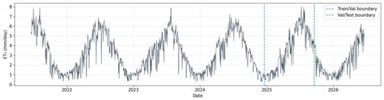
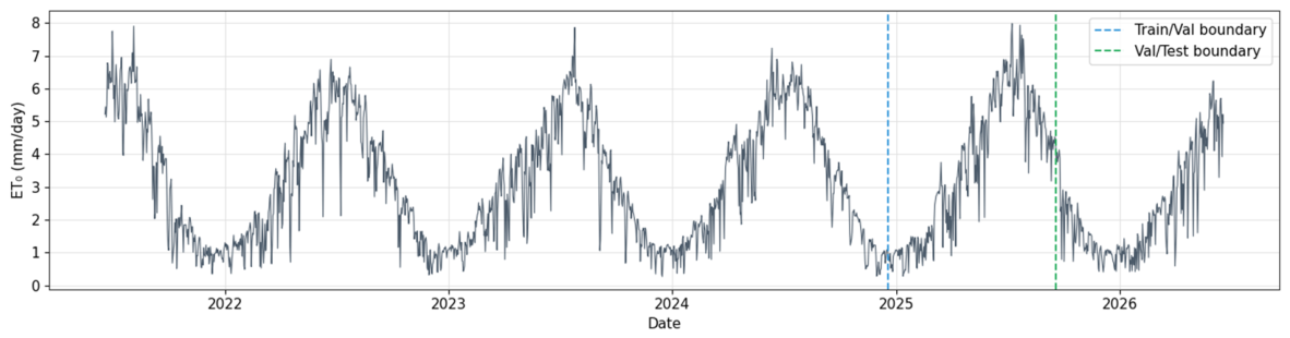
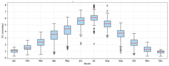
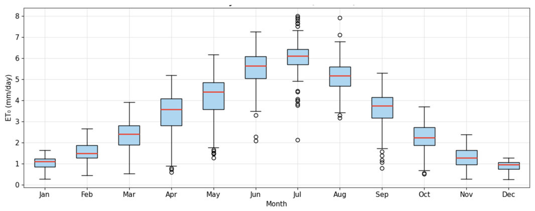
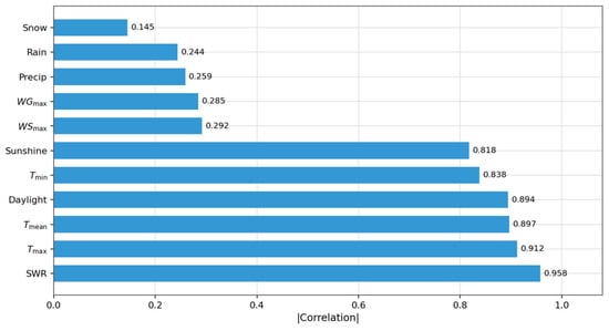
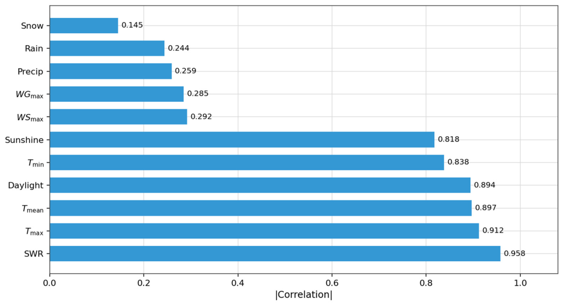
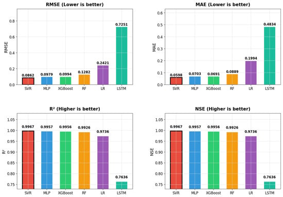
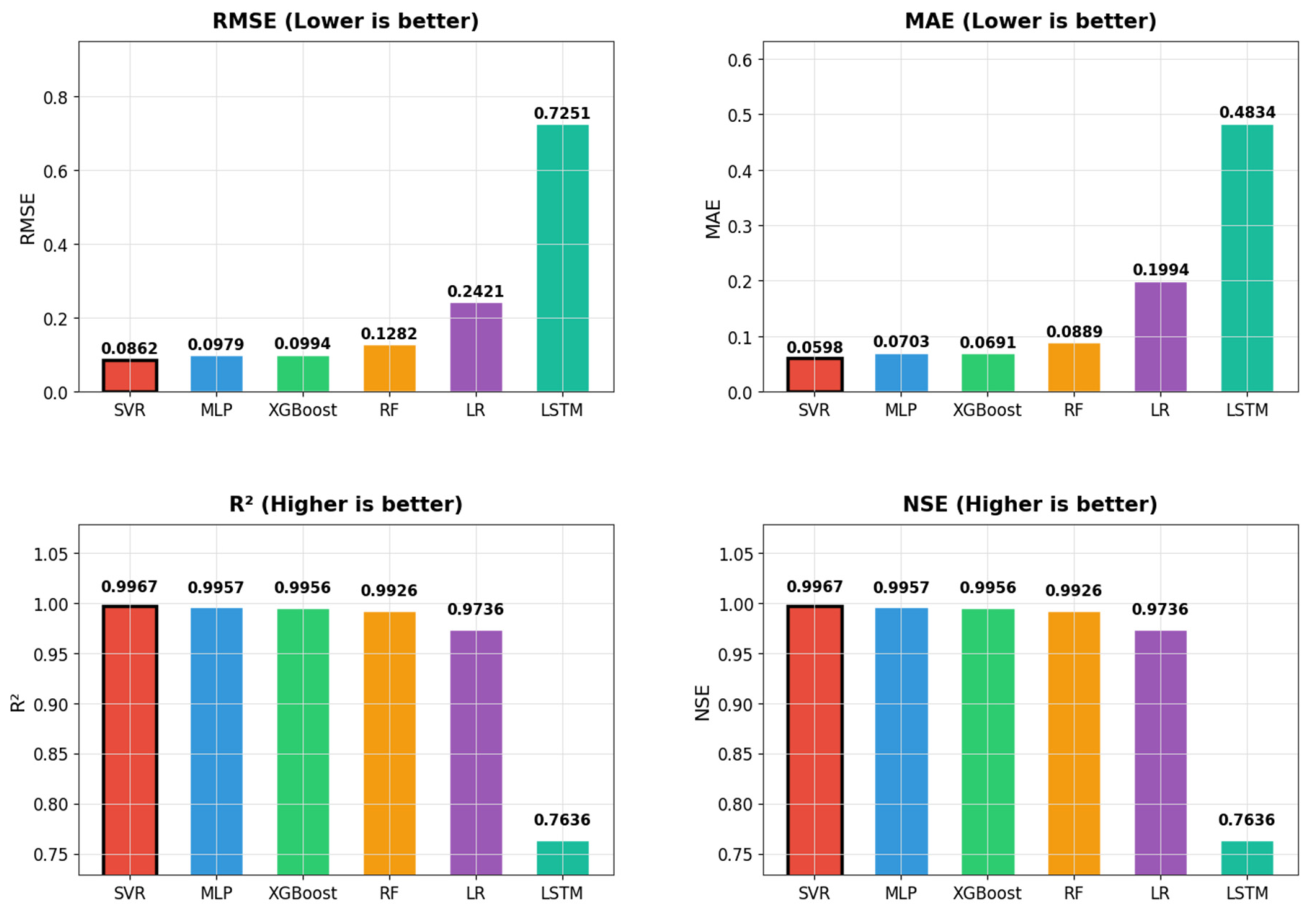
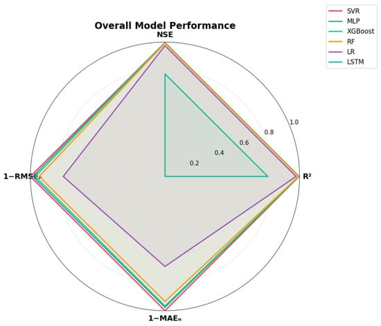
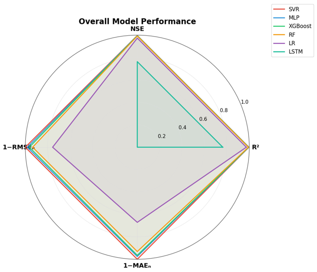
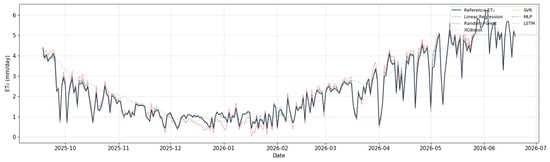
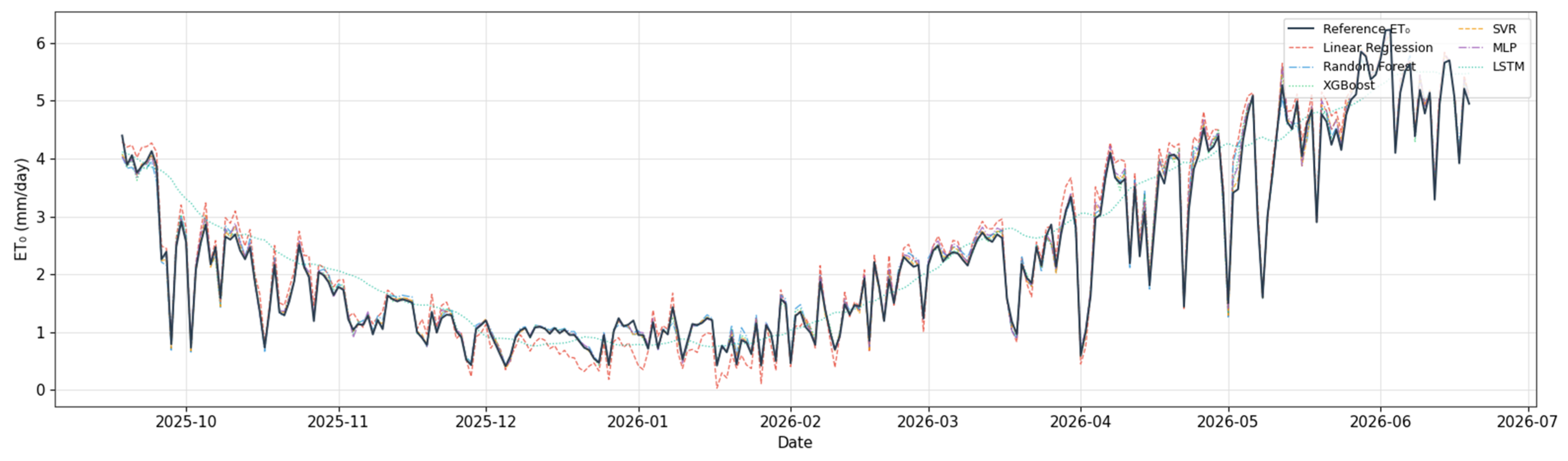
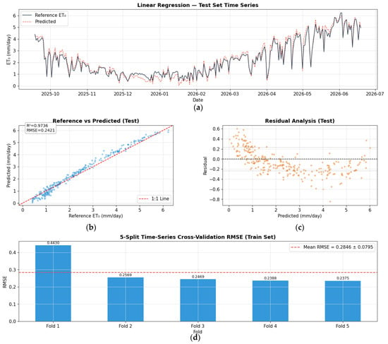
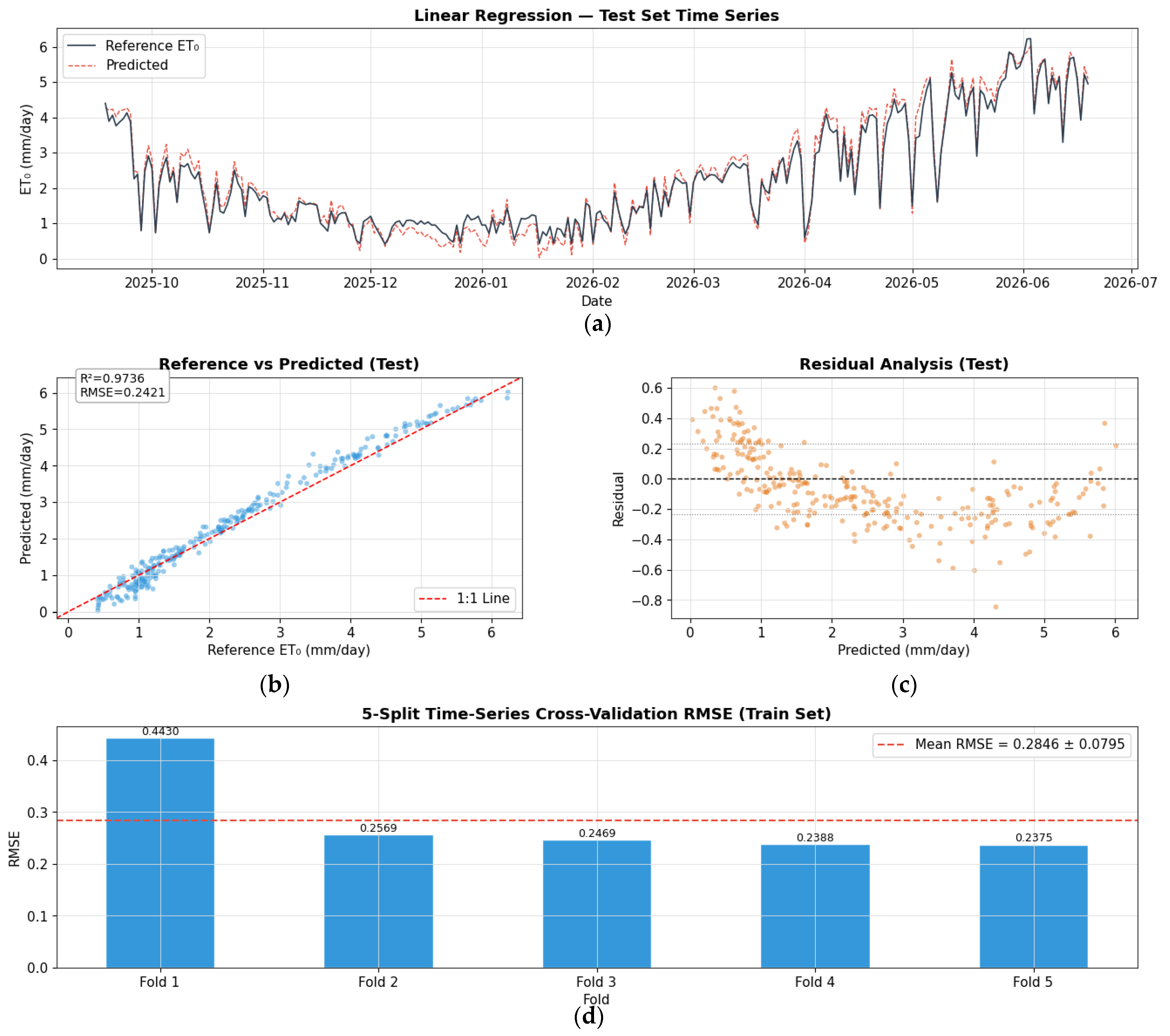
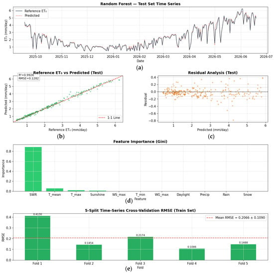
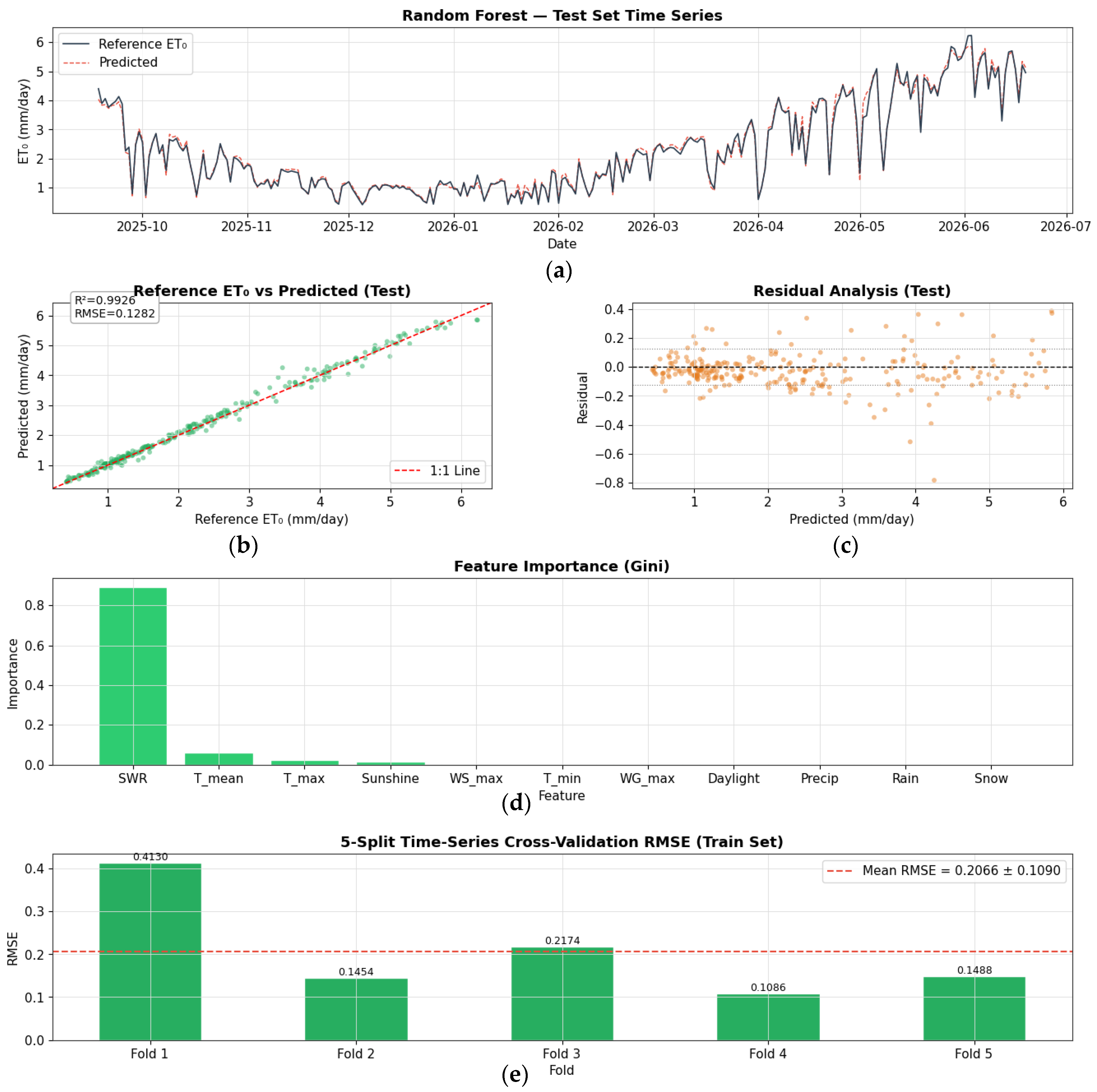
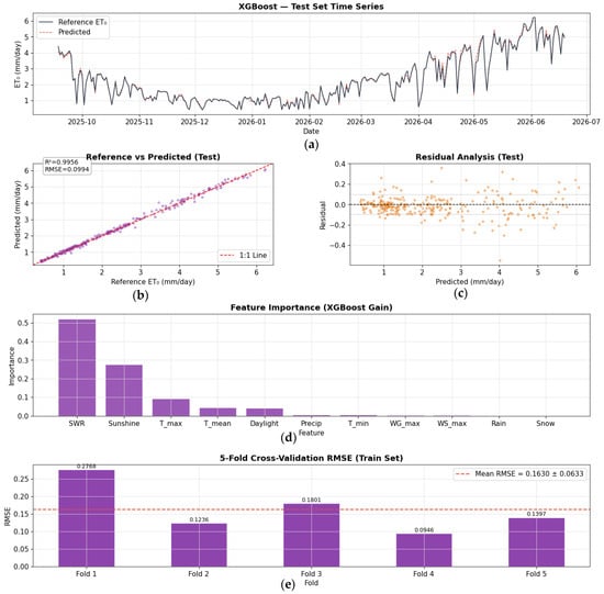
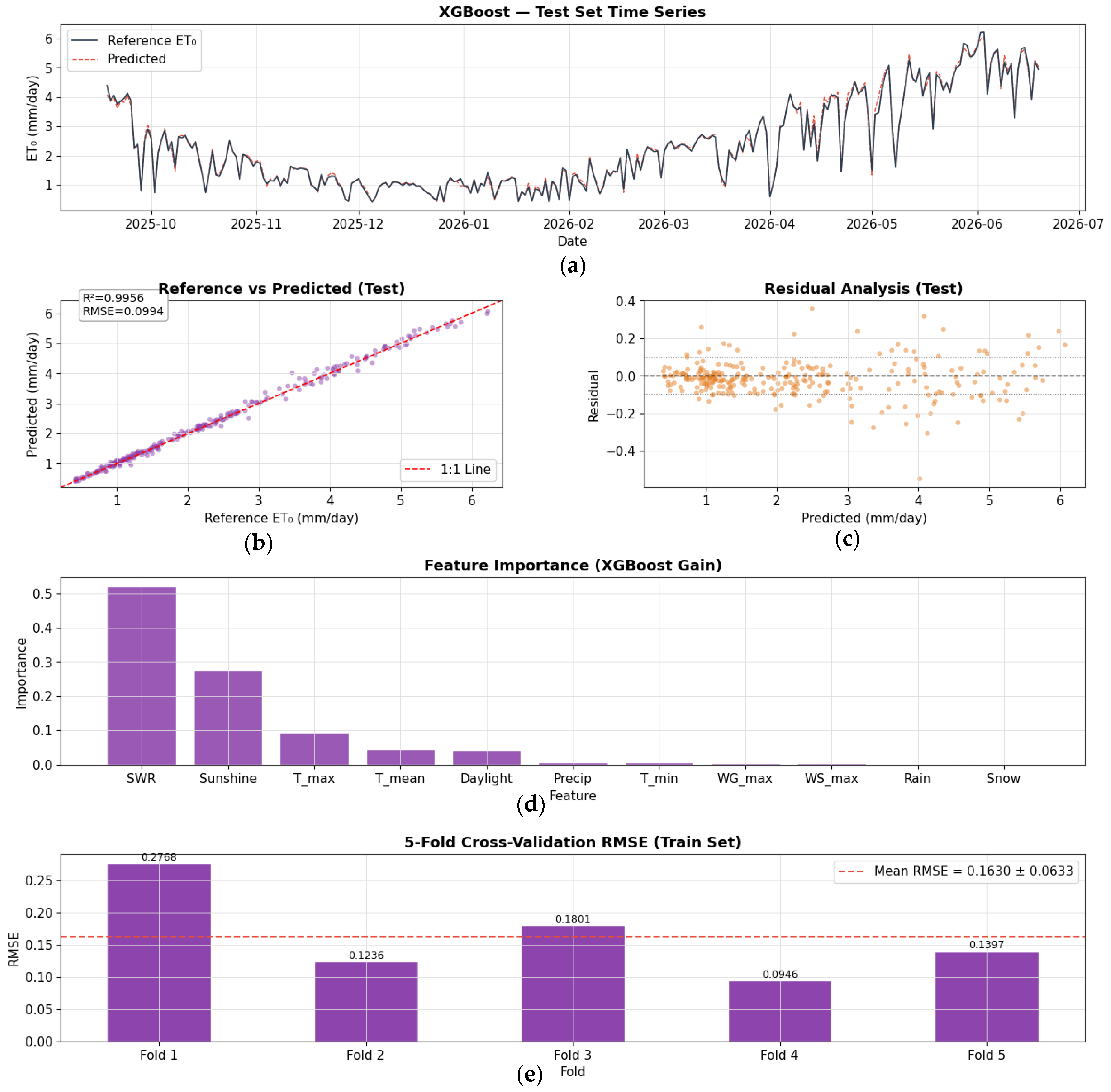
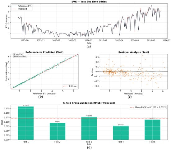
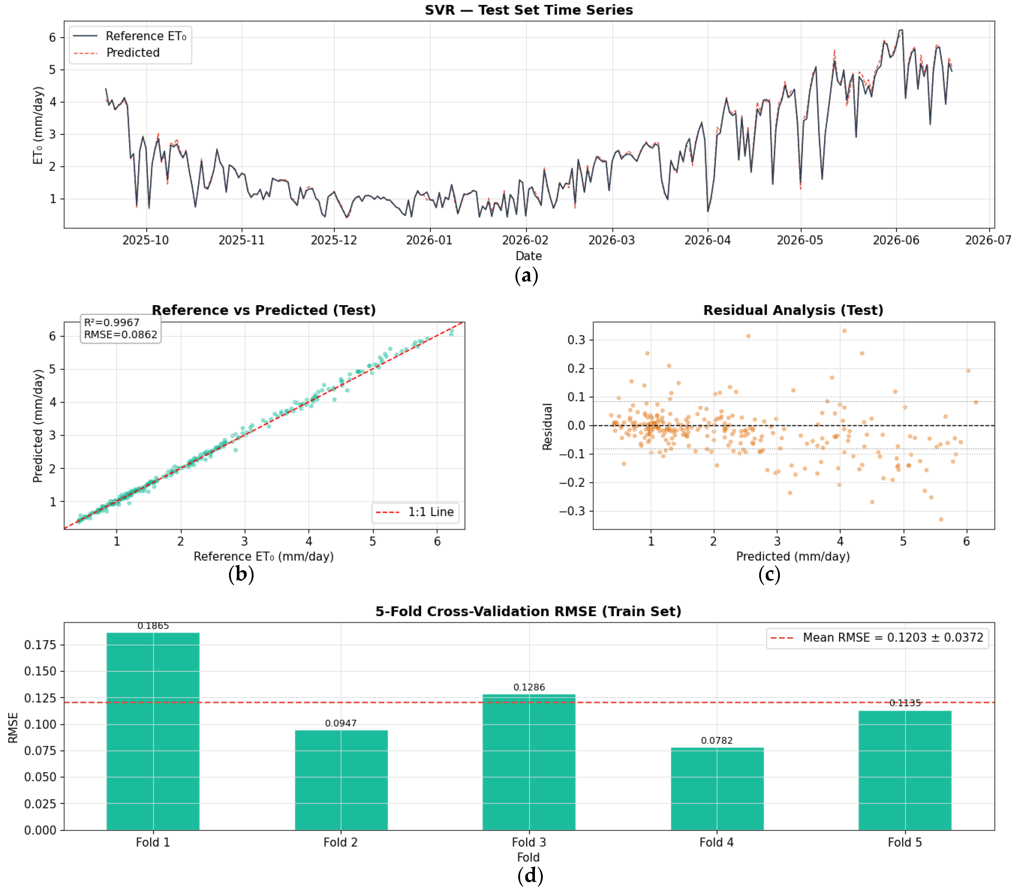
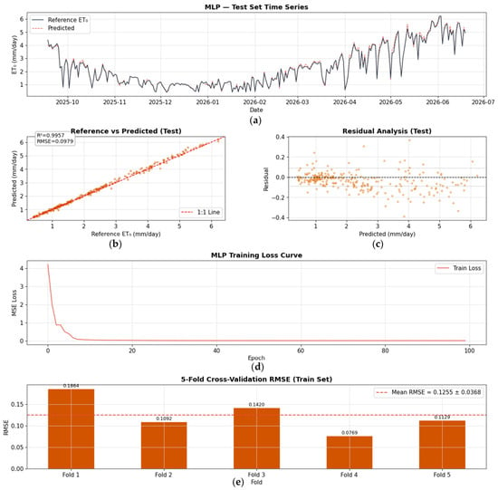
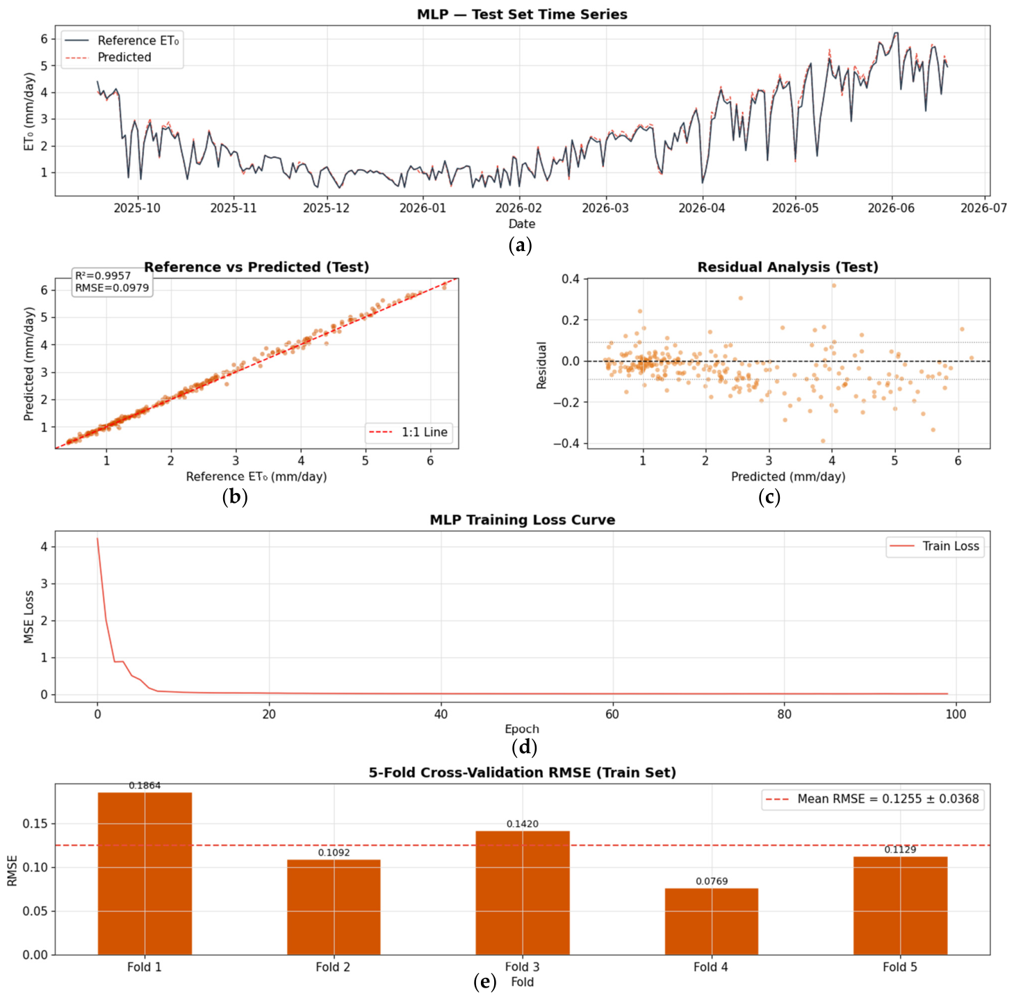
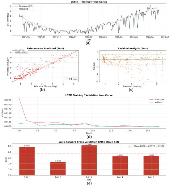
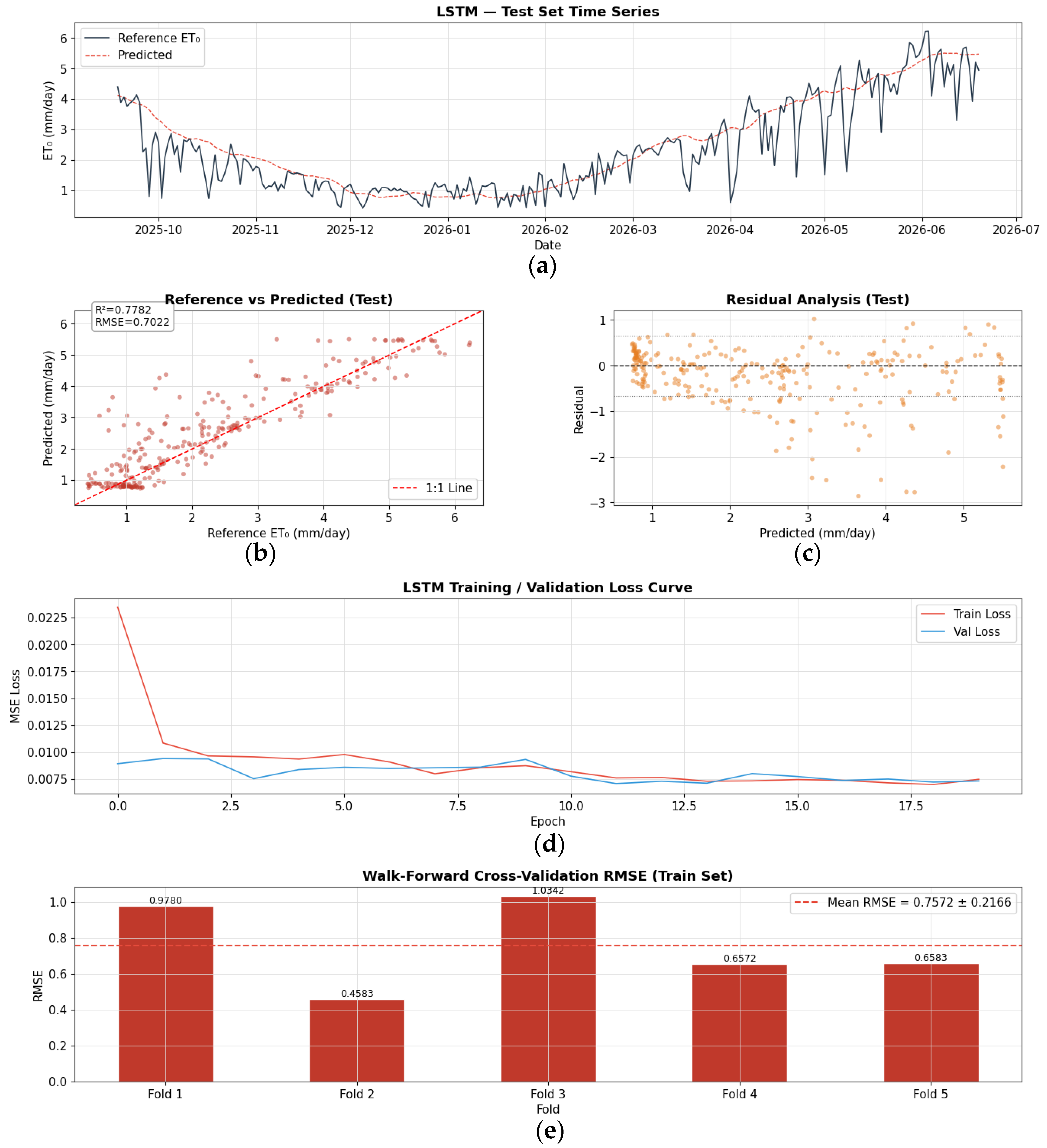
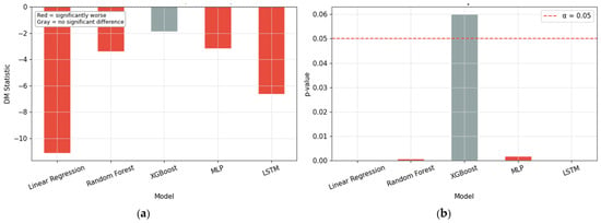
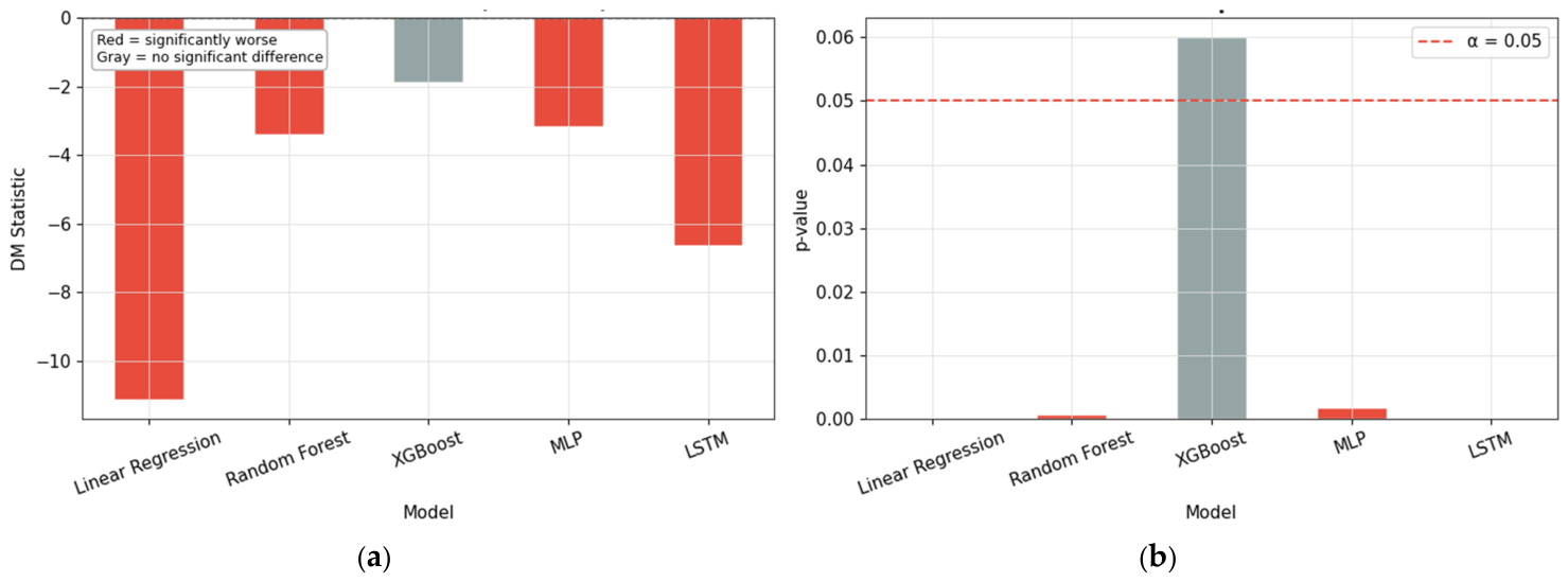
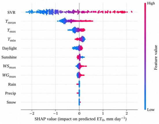
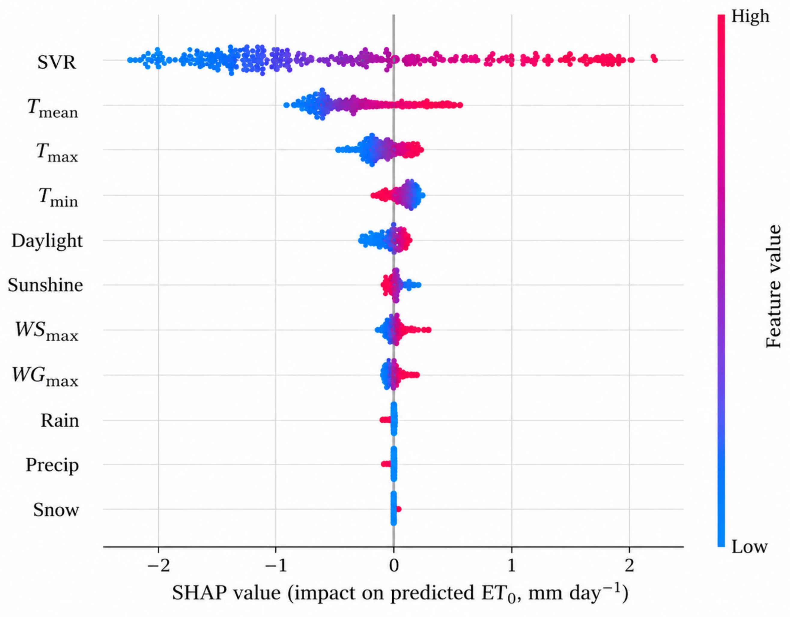

Disclaimer/Publisher’s Note: The statements, opinions and data contained in all publications are solely those of the individual author(s) and contributor(s) and not of MDPI and/or the editor(s). MDPI and/or the editor(s) disclaim responsibility for any injury to people or property resulting from any ideas, methods, instructions or products referred to in the content. |
© 2026 by the authors. Licensee MDPI, Basel, Switzerland. This article is an open access article distributed under the terms and conditions of the Creative Commons Attribution (CC BY) license.