


Abstract
Flood seasonality strongly influences flood risk and its management worldwide. Anthropogenic climate change and land-surface human activities are widely recognized as the two major drivers of its evolution, yet their relative contributions remain poorly quantified. In this study, the factorial experiment design of the Inter-Sectoral Impact Model Intercomparison Project (ISIMIP) was used to disentangle the individual and combined effects of these two drivers on global flood seasonality. Using observation-driven ISIMIP2a simulations, the ability of the ISIMIP framework to reproduce two key seasonality metrics—mean flood timing and flood timing concentration—was first evaluated. Historical and future changes in flood seasonality under RCP6.0 and RCP8.5 were then assessed at multiple spatial scales, including global grid cells, 32 major river basins, and Köppen–Geiger climate zones. Quantitative results show that north of 40° N, under the influence of land-surface human activities, the proportion of grid cells exhibiting earlier mean flood timing under RCP6.0 increases from 54.43% (climate-only) to 65.76%, with the largest change observed in the cold climate zone (median: −0.0708). In contrast, the tropical zone shows a delayed trend (median: +0.0051). Spatially, a pronounced polarization pattern emerges: high-latitude cold regions experience widespread earlier and more dispersed flood timing, while low-latitude tropical regions exhibit later and more concentrated flood timing. At the basin scale, under RCP8.5, the Pearl River Basin shows the strongest delay (ΔF = +0.1356), whereas the St. Lawrence River Basin shows the strongest advance (ΔF = −0.07445). Land-surface human activities amplify or even reverse the direction of changes in mean flood timing. When human activities are included, 31 out of 32 major basins exhibit earlier flood timing, with seven basins reversing from delay to advance. The anthropogenic climate change signal emerges over most of the globe during the first half of the 21st century, and the timing of emergence is closely linked to the warming threshold. This study reveals the modulating role of land-surface human activities in the evolution of flood seasonality and quantifies the emergence time and warming conditions associated with the anthropogenic signal, providing a scientific basis for basin-scale flood-risk management and climate adaptation strategies.
1. Introduction
Floods account for nearly half of all natural disasters worldwide, and their impacts have intensified over recent decades [1]. As one of the most destructive natural hazards, floods cause an average of 6711 deaths and USD 36.1 billion in annual global losses [2,3,4,5,6]. In extreme single years, national-scale losses can approach or even exceed this global multi-year annual average: the 2020 floods in China alone caused 279 deaths or missing persons, affected 78.61 million person-times of population, and resulted in direct economic losses of approximately USD 37.25 billion (CNY 266.98 billion) [7,8]. Under continuing climate change and human intervention, the population exposed to floods is expected to increase further [9,10,11]. Flood seasonality, which describes the intra-annual distribution of flood occurrence and reflects hydroclimatic and catchment conditions [12], is commonly characterized by mean flood timing and flood timing concentration [13]. Understanding flood seasonality is crucial for identifying flood-generation mechanisms, improving hydrological forecasting, supporting water resources management, and revealing hydrological extremes under climate change [14,15,16,17,18,19,20,21,22].
Previous studies have documented strong spatial contrasts in flood seasonality across continents. In the United States, floods generally occur in winter along the western coastal region, in late spring to early summer across the Rocky Mountains and Midwest, and are highly concentrated in snowmelt-dominated areas [23]. In Europe, flood occurrence is typically concentrated in winter in the west and Mediterranean region, in spring in the northeast, and in summer in the Alpine region [24,25]. In Africa, seasonality patterns differ among climatic regions, with winter flooding in the north and south, summer flooding in West Africa, and spring to early-summer flooding in Central Africa [26]. In China, flood seasonality exhibits marked north–south contrasts and generally high concentration, with distinct timing differences among the major hydroclimatic regions [27,28].
More recently, several studies have extended flood seasonality analysis to the global scale. Fang et al. [29] analyzed flood timing at 6167 gauging stations for 1970–2010 using circular statistics and trend testing, identifying earlier floods in snowmelt-dominated regions of North America and Europe and delayed floods in monsoon-dominated regions. Torre Zaffaroni et al. [30] combined global surface water and flood-event datasets to map flood timing worldwide and concluded that climate, rather than topography, is the dominant controller of flood timing. Renard et al. [31] reconstructed 180 years of seasonal floods and heavy precipitation at the global scale and documented strong spatial heterogeneity in their coupling. Ridolfi et al. [32] used a global inventory of flood events to show that seasonal flood changes differ markedly among seasons and regions and identified soil moisture as a major driver. These studies share two common limitations: they are either constrained by the spatial distribution of gauging stations or rely on statistical attribution, so that the effects of climatic forcing and land-surface human activities on flood seasonality remain entangled, and the timing at which the anthropogenic signal emerges from natural variability has not been quantified for flood seasonality metrics. The factorial experiment design of ISIMIP provides a way forward: because paired simulations that differ only in the presence of land-surface human activities are available under identical climate forcing, the individual contributions of anthropogenic climate change and land-surface human activities can be separated by construction, and the long 1861–2099 simulation span enables a formal time-of-emergence analysis. The present study exploits precisely these two capabilities.
Despite these important advances, three major gaps remain. First, due to the highly uneven spatial distribution of hydrometric stations, observational assessments of flood seasonality remain incomplete in many regions, especially in high latitudes, tropical rainforests, and arid areas [29,30]. Second, the ability of hydrological and climate models to reproduce flood seasonality has rarely been evaluated systematically. Although many studies have examined model performances for flood magnitude, frequency, and duration [33,34,35], it remains unclear whether current model ensembles can reliably simulate the timing and concentration of flood occurrence, which is essential for credible future projections. Third, the relative contributions of anthropogenic climate change and land-surface human activities to changes in flood seasonality have not yet been quantified rigorously. Existing studies have mainly relied on statistical attribution [29,32] and have seldom separated the effects of climatic forcing from those of land-use change, reservoir regulation, and water management. As a result, key questions remain unresolved, including how flood seasonality may evolve under future scenarios and when anthropogenic signals will emerge from natural variability [36,37].
To address these gaps, this study develops a multi-scenario, multi-scale framework to assess model performance, quantify changes in flood seasonality, and detect the emergence of anthropogenic climate signals. Specifically, it addresses three research questions: (RQ1) How reliably can the ISIMIP model ensemble reproduce the observed mean flood timing and flood timing concentration at the global scale? (RQ2) What are the individual and combined effects of anthropogenic climate change and land-surface human activities on flood seasonality at the global, basin, and climate-zone scales? (RQ3) When, and at what level of global warming, do anthropogenic signals in flood seasonality emerge from natural variability? Operationally, these questions are addressed through four objectives: (1) evaluate the ability of ISIMIP hydrological and climate model combinations to reproduce historical mean flood timing and flood timing concentration using global streamflow observations; (2) characterize historical and future changes in flood seasonality at the global, basin, and climate-zone scales; (3) disentangle the respective contributions of anthropogenic climate change and land-surface human activities using paired factorial simulations; and (4) identify the time of emergence (ToE) and associated warming level of anthropogenic signals in flood seasonality using a signal-to-noise framework. The results are expected to improve process-based understanding of flood-regime reorganization under global change and provide useful information for flood-risk management and climate adaptation. Throughout this study, “anthropogenic climate change” refers to changes in climatic forcing represented by the paired historical and RCP simulations relative to the pre-industrial control simulation, and “land-surface human activities” refers specifically to the direct human modification of the land-surface water cycle represented by the ISIMIP scenario pairs—namely human water use (irrigation and industrial and domestic abstraction), reservoir regulation, land-use change, and time-varying population and socio-economic development. Anthropogenic pressures that are not implemented as switchable forcings in the ISIMIP factorial experiments—such as pollution, urbanization intensity, and settlement density—are not explicitly separated; their potential roles are discussed as limitations in Section 4. The framework developed here is directly transferable to other flood-regime metrics (e.g., flood magnitude, frequency, and duration), to other hydroclimatic extremes (e.g., low flows and droughts), and to future generations of factorial simulations (e.g., ISIMIP3), providing a reusable template for separating climatic and anthropogenic influences on hydrological change. The findings are directly relevant to the Sustainable Development Goals: to SDG 13 (Climate Action), by quantifying when anthropogenic signals in flood regimes emerge and at what warming levels; to SDG 11 (Sustainable Cities and Communities), through the implications of a shifting flood calendar for urban flood-risk management; and to SDG 6 (Clean Water and Sanitation), through the consequences of shifting flood timing for reservoir operation, water allocation, and water security.
2. Data and Methods
The overall workflow of this study is illustrated in Figure 1 and consists of four modules. In the data module, daily streamflow observations (GSIM, GSCD, and additional Chinese records) and the ISIMIP2a/ISIMIP2b daily runoff simulations-organized as paired runs with and without land-surface human activities-are assembled, quality-controlled, and regirded to a common 0.5° grid. In the flood seasonality module, the annual maximum daily streamflow and its occurrence date are extracted from each time series, and the two seasonality metrics (mean flood timing and flood timing concentration) are computed with circular statistics at the grid-cell, basin, and climate-zone scales.
Figure 1.
Flowchart of the modeling and analysis framework. Solid boxes indicate data sources, dashed boxes processing steps, and colored arrows the two attribution branches (climate-only vs. combined climate–human).
Thirty-two major river basins were selected for the basin-scale analysis, following four criteria. (i) Size: A drainage area large enough to be resolved by the 0.5° ISIMIP grid, in practice of the order of 105 km2 or more. (ii) Identifiability: The basin can be delineated as a single contiguous unit in the river-routing network and basin mask used by the ISIMIP simulations, so that gridded runoff can be aggregated without ambiguity. (iii) Representativeness: The set covers all four Köppen–Geiger climate zones used here and all continents with major river systems. (iv) Consistency with previous work: The set overlaps the large basins used in earlier global assessments, including the seventy basins mapped by Oki et al. [38]. Basins satisfying (i) and (iii) but not (ii)—that is, basins that the routing network merges with a neighboring outlet—were not analyzed separately. This applies in particular to the Tocantins River (ca. 9 × 10⁵ km2), which is a continental-scale basin but is aggregated with the Amazon outlet in the routing network used here, so that its gridded runoff cannot be isolated without introducing an arbitrary delineation. The exclusion of such basins affects the number of basins analyzed but not the grid-cell or climate-zone results, which are computed independently of the basin delineation.
In the validation module, observation-driven ISIMIP2a simulations are evaluated against GSIM observations, and ISIMIP2b climate-forced simulations are in turn evaluated against ISIMIP2a, establishing the credibility of the model chain for seasonality simulation.
In the attribution module, six paired comparison scenarios (S1–S6) are constructed from the factorial ISIMIP design; the relative change metric ΔF is decomposed into climate-driven and human-driven components, and the signal-to-noise framework is applied to detect the time of emergence and the associated global warming level of anthropogenic signals, with multi-model agreement assessed by the 50% ensemble criterion.
2.1. Streamflow Observations
Daily streamflow observations were primarily obtained from the Global Streamflow Indices and Metadata Archive (GSIM) [39], supplemented by the Global Streamflow Characteristics Dataset (GSCD) and additional gauged records from hydrological agencies in China. GSIM integrates 12 national and research databases and, after quality control and removal of duplicate stations, provides daily streamflow time series for 30,959 stations worldwide for the period 1804–2016. GSCD covers 20,346 stations and was used to supplement areas with sparse gauge coverage. For China, additional daily streamflow observations were collected for 398 stations across the Yangtze, Yellow, Pearl, Huaihe, Tarim, and Poyang Lake basins, spanning 1915–2019, as well as annual maximum discharge series for 58 stations in Guangdong Province during 1951–2014.
To evaluate the accuracy of ISIMIP simulations, 12,533 stations with good-quality daily records during 1971–2005 were selected. These observations were used as the benchmark for evaluating the simulated mean flood timing and flood timing concentration.
2.2. ISIMIP Simulations
This study used daily runoff simulations from phase 2 of the Inter-Sectoral Impact Model Intercomparison Project (ISIMIP2), including ISIMIP2a and ISIMIP2b, at a spatial resolution of 0.5° × 0.5° [40]. ISIMIP2a was used to evaluate model performance for historical flood seasonality. In ISIMIP2a, six global hydrological models (DBH, H08, LPJmL, MATSIRO, PCR-GLOBWB, and WaterGAP2-2c) were driven by six observation-based meteorological forcing datasets, including Princeton, GSWP3, and WATCH-WFDEI, to generate daily runoff series for 1971–2016.
ISIMIP2b was used for historical and future analyses. It includes simulations from eight hydrological models forced by four bias-corrected CMIP5 global climate models (GFDL-ESM2M, HadGEM2-ES, IPSL-CM5A-LR, and MIROC5), covering 1661–2099. The dataset includes the historical period (1861–2005) and future projections under RCP6.0 and RCP8.5 (2006–2099). All climate model outputs were bias-corrected before being used to force the hydrological models.
Both ISIMIP2a and ISIMIP2b provide simulations with and without land-surface human activities, allowing the separation of climate and human influences. In ISIMIP2a, the nosoc scenario excludes human water use, reservoir regulation, and land-use change, whereas the varsoc scenario includes temporally varying population, GDP, land use, and socio-economic development. In ISIMIP2b, historical simulations use the histsoc scenario, future simulations use the 2005soc scenario, and pre-industrial control runs use the 1860soc scenario. Comparisons among these simulations make it possible to quantify the effects of anthropogenic climate change and land-surface human activities on flood seasonality.
In addition, ISIMIP2b near-surface air temperature (tas) data were used to calculate global mean warming. ISIMIP2a/ISIMIP2b, rather than ISIMIP3, were used for three reasons. First, the attribution design requires paired simulations with and without land-surface human activities under identical climate forcing; at the time this study was designed and the data were processed, ISIMIP2b provided the complete and internally consistent set of such scenario pairs (nosoc/histsoc/2005soc/1860soc) across all eight hydrological models and four bias-corrected GCMs used here. Second, the ISIMIP2b archive covers the continuous 1661–2099 period, including the pre-industrial control baseline that is essential for the signal-to-noise and time-of-emergence analysis. Third, using ISIMIP2a for the observation-driven evaluation and ISIMIP2b for the attribution guarantees methodological consistency between the validation and projection components of the framework. These data were derived from the same four CMIP5 models for the piControl, historical, RCP6.0, and RCP8.5 simulations and have daily temporal resolution and 0.5° × 0.5° spatial resolution. These components were selected because they represent the dominant direct pathways through which human activities alter the timing and concentration of riverine floods at the global scale: reservoir regulation stores and redistributes flow in time and can shift flood peaks by weeks; irrigation and water abstraction modify the catchment water balance, baseflow, and soil-moisture preconditioning; land-use change alters infiltration, evapotranspiration, and runoff generation; and population and socio-economic development determine the intensity and spatial distribution of these water demands. Collectively, they describe the first-order, direct anthropogenic modification of runoff generation and routing at the 0.5° global scale. It should be noted that the factorial design quantifies the effect of land-surface human activities as represented in the ISIMIP scenario pairs. Anthropogenic pressures that are not implemented as switchable forcings in these experiments—including pollution, urbanization intensity, and settlement density—are not explicitly separated; where such pressures co-vary with the represented components (e.g., urban expansion with land-use change), their effects are partially, but incompletely, absorbed into the estimated human-effects term.
2.3. Climate Classification
To examine the climatic dependence of flood seasonality, the Köppen–Geiger climate classification system [41,42] was adopted (as shown in Figure 2). This system classifies the globe into five major climate types-tropical (A), arid (B), temperate (C), cold (D), and polar (E)-based on temperature, precipitation, and their seasonality. The 1 km global Köppen–Geiger maps [43] were used, including the historical classification for 1980–2016 and the future classification under RCP8.5 for 2071-2100. The most pronounced changes in the southern hemisphere are the expansion of arid and semi-arid (B) classes at the expense of temperate (C) classes over southern Africa, southern South America and Australia, together with a poleward shift in the temperatecontinental boundary. In the northern high latitudes, cold (D) classes contract and shift poleward. Of these transitions, the expansion of arid classes in the subtropics and the poleward shift in the temperate–continental boundary are the ones most directly relevant to the flood seasonality changes discussed in Section 3.2 and Section 3.3, because they coincide with the regions in which the concentration of flood timing changes most strongly.
Figure 2.
Global Köppen–Geiger climate classification map at 1 km resolution [43]. (a) Historical period (1980–2016); (b) future period (RCP8.5, 2071–2100).
2.4. Quantification of Changes in Flood Seasonality
Flood seasonality is typically driven by multiple mechanisms, with different mechanisms dominating in different seasons. To evaluate the seasonal characteristics of floods, the circular-statistics method has been widely adopted in the literature [14,21,44]. In this study, a flood event is defined as the annual maximum daily streamflow (AMDF), and its occurrence date—the day of the year on which the annual maximum occurs—is taken as the flood day. This definition is used consistently throughout the study and was adopted for three reasons: (i) it is the standard index used in circular-statistics-based flood seasonality studies [14,21,44], ensuring comparability with previous work; (ii) daily streamflow is the finest resolution available consistently across the GSIM observations and all ISIMIP simulations; and (iii) the date of the single-day annual maximum maps directly onto the circular-statistics framework without additional window-definition assumptions. It should be noted that the window length affects only the delineation of the flood event around the annual maximum, and not the date of the annual maximum itself; it therefore has no first-order influence on either of the two seasonality metrics analyzed here.
First, the date of each annual flood event is converted to radians:
where Di is the day of year of the flood event in the i-th year (Di = 1,2,…,m), m is the total number of days in that year (365 for common years, 366 for leap years), and θi is the corresponding angle in radians (0∼2π).
Next, the mean cosine component and mean sine component of the flood occurrence dates are calculated as follows:
where n is the total number of years, and both and range from −1 to 1.
The mean flood timing is then computed using the following piecewise function:
Here, returns the principal value in the range −π/2∼π/2. The quadrant correction ensures that the result falls within 0∼m (i.e., 0–365 or 0–366 days), and the multiplication by m/(2π) converts radians back to days.
Finally, the flood timing concentration index (R) is defined as follows:
R is a dimensionless index ranging from 0 to 1. R = 0 indicates that flood events are uniformly distributed throughout the year (no seasonality), while R = 1 indicates that all flood events occur on the same day (perfect seasonality). A larger value of R indicates stronger flood seasonality.
2.5. Experimental Design
Flood events and their occurrence dates were defined as described in Section 2.4 (the annual maximum daily streamflow and its day of occurrence). Flood seasonality was quantified using two indices: mean flood timing and flood timing concentration. To compare flood seasonality between two periods, we used the relative change metric. For a baseline period (P1) and a target period (P2), the change in a flood seasonality metric (ΔF) was quantified from the difference between its mean values during the two periods. The relative change in a flood seasonality metric F between a baseline period P1 and a target period P2 is defined as follows:
where (P1) and (P2) denote the mean values of the metric over the two periods. Using the six comparison scenarios defined above, ΔF is decomposed into a climate-driven component and a land-surface human-activities component:
where ‘soc’ denotes the simulation pairs that include land-surface human activities (S1, S3, S5) and ‘nosoc’ the pairs that exclude them (S2, S4, S6). ΔFclimate quantifies the change attributable to anthropogenic climate forcing alone, ΔFtotal the combined change, and ΔFhuman the additional contribution of land-surface human activities, with the climate–human interaction term absorbed into ΔFhuman by construction.
ΔFhuman = ΔFtotal − ΔFclimate
Six comparison scenarios were designed to separate the effects of anthropogenic climate change and land-surface human activities:
S1: piControl vs. Historical, including land-surface human activities.
S2: piControl vs. Historical, excluding land-surface human activities.
S3: Historical vs. RCP6.0, including land-surface human activities.
S4: Historical vs. RCP6.0, excluding land-surface human activities.
S5: Historical vs. RCP8.5, including land-surface human activities.
S6: Historical vs. RCP8.5, excluding land-surface human activities.
Here, piControl refers to the pre-industrial baseline period (1861–1890), Historical to the historical reference period (1976–2005), and RCP6.0 and RCP8.5 to the future period 2070–2099. Scenarios S1 and S2 were used to detect already emerged historical changes, whereas S3–S6 were used to assess future changes.
2.6. Detection of Anthropogenic Climate Signals
To quantitatively identify the emergence of anthropogenic climate signals in flood seasonality, this study adopts the signal-to-noise ratio (SNR) framework [37,45].
2.6.1. Definition of Signal and Noise
The signal (S(t)) is defined as the difference between the 30-year moving average of a flood seasonality metric (F) during 1861–2099 and the long-term mean of the same metric under the pre-industrial control simulation (piControl). The 30-year averaging window was adopted for three reasons. First, it corresponds to the standard climatological normal period defined by the World Meteorological Organization, which provides a physically interpretable reference. Second, it is long enough to suppress interannual-to-decadal internal variability, yet short enough to resolve the centennial evolution of the anthropogenic signal within the 1861–2099 simulation period. Third, averaging windows of similar length have been used in previous time-of-emergence studies [36,37,45], ensuring comparability of the ToE estimates.
where is the 30-year moving average centered at year t, and is the mean value of F over the entire piControl period.
The noise (N) is defined as n times the standard deviation of F in the piControl simulation:
where σpiControl is the standard deviation of F in the piControl period. Following Wieder et al. [46], the scaling factor n is set to 0.5 for the flood timing concentration index (R) and to 2 for the mean flood timing in order to balance sensitivity and specificity in signal detection. It should be noted that the emergence results are governed primarily by the signal-to-noise criterion rather than by the window length itself: the signal is defined relative to the piControl distribution, and emergence is only declared once the criterion is satisfied for at least 20 consecutive years. A different window length would alter the degree of smoothing applied to the signal, but not the direction or the spatial pattern of the detected emergence, because the underlying scenario separation is monotonic and substantially larger than the variation introduced by the smoothing.
N = n ⋅ σpiControl
2.6.2. Signal-to-Noise Ratio and Emergence Condition
The signal-to-noise ratio is then computed as follows:
An anthropogenic climate signal is considered to have emerged when
SNR(t) > 1
The 20-consecutive-year persistence requirement was imposed to reduce the risk of mistaking transient SNR excursions—driven by internal climate variability rather than by the forced response—for genuine signal emergence. Requiring the SNR to exceed 1 for at least 20 consecutive years within the same moving window ensures that the detected signal is persistent and stable, in line with the persistence considerations adopted in previous emergence-detection studies [36,37,45]. The threshold is also consistent with the interpretation of the 30-year reference period used for the signal, since a persistence requirement of at least two-thirds of a reference period effectively excludes isolated excursions while retaining the ability to detect a sustained forced response. This can be expressed as follows:
where 1{ ⋅ } is the indicator function.
2.6.3. Time of Emergence (ToE) and Global Temperature of Emergence (GToE)
The time of emergence (ToE) is defined as the central year of the first 30-year window that satisfies both of the following conditions:
The corresponding global temperature of emergence (GToE) is the global mean warming level (derived from ISIMIP2b temperature data) at the ToE.
2.6.4. Multi-Model Ensemble Processing
For a multi-model ensemble, a detectable signal is considered to exist at a given grid cell or region if more than 50% of the individual models satisfy the emergence conditions [47]. The multi-model ToE (or GToE) is then taken as the median of the ToE (or GToE) values across those models:
where detected = {m:ToEm exists}, and the condition ∣detected∣ > 0.5 ⋅ ∣∣ must hold. Otherwise, no reliable emergence is identified for that ensemble [48].
ToEensemble = median{ToEm:m ∈ detected}
3. Results
3.1. Evaluation of ISIMIP Performance in Simulating Flood Seasonality
To ensure the robustness of the subsequent attribution and projection analyses, the ability of ISIMIP to reproduce flood seasonality using a two-step validation framework was evaluated. First, GSIM observations were compared with observation-driven ISIMIP2a simulations for 1971–2005 to assess hydrological model performance. Second, ISIMIP2a was compared with climate-forced ISIMIP2b simulations for the same period to evaluate the extent to which climate model forcing preserved the seasonality characteristics reproduced by observation-driven simulations. The evaluation was conducted at the global grid-cell scale, across 32 major river basins (as shown in Figure 3), and within Köppen–Geiger climate zones.
Figure 3.
Distribution of 32 major large river basins worldwide. Basins analysed in this study are highlighted in yellow; remaining land areas are shown in grey.
In the first validation step, 909 GSIM stations located close to mapped river channels were selected as reference points, as shown in Figure 4. ISIMIP2a reproduced the broad spatial patterns of both mean flood timing and flood timing concentration. Regions such as India and Mexico showed flood occurrence concentrated in June–August, whereas Brazil and southern Africa were dominated by January–March floods, which is in good agreement with observations. The spatial pattern of flood timing concentration was also captured reasonably well, although regional discrepancies remained. Model skill is assessed in terms of the spatial pattern of the seasonality metrics rather than their point-wise absolute accuracy. Two aspects of the evaluation are relevant in this respect. First, in addition to R2, the slopes of the regression between simulated and observed metrics are reported (0.62 for mean flood timing and 0.52 for flood timing concentration). Unlike correlation, the slope is sensitive to systematic bias and to the compression of the simulated range, so a slope approaching unity indicates that the model reproduces not only the spatial pattern but also the amplitude of the observed seasonality. Second, and more importantly for the interpretation of the attribution results, all attributions reported below are computed from differences between paired simulations of the same model. Because both members of each pair share the same model structure and the same systematic biases, the bias largely cancels in the difference, so that the reliability of the climate–human decomposition does not depend on the absolute accuracy of the simulated flood timing. These results indicate that ISIMIP2a captures the first-order spatial variability of observed flood seasonality, despite a tendency to simulate slightly later flood timing and somewhat stronger concentration.
Figure 4.
Global distribution of flood seasonality characteristics and validation of ISIMIP simulations against GSIM observations for the period 1971–2005. Panels (a–c) show the spatial distribution of mean flood timing derived from GSIM, ISIMIP2a, and ISIMIP2b, respectively, while panels (d–f) show the corresponding flood timing concentration (R). Panels (g,h) present scatter plots comparing station-based mean flood timing and flood timing concentration between GSIM and ISIMIP2a, and panels (i,j) show comparisons between ISIMIP2a and ISIMIP2b at the global grid scale. Blue lines indicate the boundaries of 32 major river basins worldwide. In the scatter plots, R2 and p denote the coefficient of determination and the significance level from linear regression, respectively.
The second validation step showed that ISIMIP2b preserved these characteristics with high fidelity. The spatial distributions of mean flood timing and flood timing concentration were highly consistent between ISIMIP2a and ISIMIP2b, and grid-level comparisons approached a one-to-one relationship for both indices. Regression slopes were 0.85 for mean flood timing and 0.84 for flood timing concentration, with corresponding R2 values of 0.74 and 0.77 (p < 0.05). This close agreement indicates that the use of bias-corrected climate model forcing does not substantially reduce the ability of the model ensemble to simulate flood seasonality.
Overall, the two-step validation demonstrates that ISIMIP2b reproduces the large-scale characteristics of observed flood seasonality with sufficient skill for the purposes of attribution and future projection. Although uncertainties remain at local scales, the model ensemble provides a robust basis for assessing the effects of anthropogenic climate change and land-surface human activities on flood seasonality.
These skill levels have two implications for the interpretation of the subsequent analyses. First, because the attribution and emergence analyses are based on comparisons within the same model world (paired scenarios relative to a common pre-industrial baseline) rather than on absolute agreement with observations, systematic biases in simulated flood timing tend to affect all scenario pairs similarly and largely cancel out in the relative change metrics; the factorial design is therefore internally consistent. Second, however, the moderate point-scale agreement (R2 = 0.51 for mean flood timing and 0.46 for flood timing concentration) implies that local, grid-cell-level attribution results—particularly in regions far from gauges—should be interpreted with caution. For this reason, all headline findings are reported at the global, basin, and climate-zone scales using multi-model medians and model-agreement criteria rather than at the individual grid-cell scale. The skill obtained here is comparable to that reported by Do et al. [17], and the simulated spatial pattern reproduces the observed shifts documented by Fang et al. [29]; the agreement and the differences are discussed in Section 4.
3.2. Responses of Flood Seasonality to Anthropogenic Climate Change and Land-Surface Human Activities
3.2.1. Mean Flood Timing
At the global scale, historical changes in mean flood timing relative to the pre-industrial period show pronounced spatial heterogeneity (Figure 5). In all map figures below, stippling indicates grid cells where at least 70% of the models agree on the direction of change, and the curves on the right show zonal averages (blue: excluding land-surface human activities; red: including them; solid lines: multi-model mean; shading: ±0.5 standard deviations). Under anthropogenic climate change alone, 54.84% of global land grid cells exhibit earlier flood timing, mainly in northern Canada, eastern North America, southern Europe, parts of West Asia, and southern Africa, whereas 45.16% exhibit delayed flood timing, particularly in the Rocky Mountains, eastern Russia, southern India, and parts of Southeast Asia. When land-surface human activities are included, the proportion of grid cells with earlier flood timing increases to 59.56%, indicating that human influences generally reinforce the tendency toward earlier floods while also modifying the regional response pattern.
Figure 5.
Multi-model median changes in mean flood timing under the historical, RCP6.0, and RCP8.5 scenario pairs. Panels (a,c,e): climate-driven changes; Panels (b,d,f): combined climate- and human-driven changes. Stippling and zonal curves are as defined in Section 3.2.1.
This large-scale behavior persists under future warming, although the response depends on the emission pathway. Under RCP6.0 in Figure 5, the spatial pattern broadly resembles that of the historical period but the magnitude of change increases substantially, especially north of 30° N. In the climate-only simulations, 54.43% of grid cells show earlier flood timing, whereas this fraction rises to 65.76% when land-surface human activities are included. Under RCP8.5, the climate-only response becomes more spatially contrasted, with only 48.73% of grid cells showing earlier flood timing and delays becoming more widespread in northern Europe, Siberia, and parts of South America. However, when land-surface human activities are included, the proportion of grid cells with earlier flood timing increases again to 63.10%. These results indicate that anthropogenic climate change dominates the global-scale reorganization of flood timing.
In Figure 6, the basin-scale analysis further shows that human influences can fundamentally reshape regional flood-timing responses. During the historical period, under climate forcing alone, 16 of the 32 major basins exhibit earlier flood timing and 16 show delayed flood timing. Once land-surface human activities are included, 24 basins exhibit earlier flood timing, and several basins, including the Columbia, Irrawaddy, and Lena, shift from delayed to earlier timing. Similar behavior is found under future scenarios. Under RCP6.0, 18 basins show earlier flood timing and 14 show delayed flood timing in the climate-only simulations, whereas 31 basins show earlier flood timing when land-surface human activities are included. Under RCP8.5, climate forcing alone produces delayed flood timing in most basins, but the inclusion of human influences shifts the balance toward earlier flood timing in 23 basins. These directional reversals indicate that land and water management are not merely secondary perturbations, but can strongly alter basin-scale flood seasonality.
Figure 6.
Relative changes in mean flood timing at basin and climate-zone scales under historical and future scenarios. (a,b) Historical period (1976–2005 vs. 1861–1890); (c,d) RCP6.0 (2070–2099 vs. 1976–2005); (e,f) RCP8.5 (same period as RCP6.0). Panels (a,c,e) show area-weighted mean changes across 32 major river basins (bars).
In Figure 7, the climate-zone analysis reveals systematic differences among hydroclimatic regions. Historical changes in mean flood timing are generally small, but their sign differs among climate zones: tropical and arid regions tend to show weak delayed flood timing, whereas temperate and cold regions tend to exhibit earlier flood timing. Under future warming, these responses intensify, with the cold zone showing the strongest advance in flood timing, especially when land-surface human activities are included. Decadal trajectories further indicate that cold and temperate zones shift progressively from delayed to earlier flood timing, whereas the tropical zone maintains a more persistent tendency toward delayed flood timing. This contrast suggests that snowmelt-dominated and energy-limited environments are especially sensitive to warming-induced shifts in runoff seasonality, while flood timing in low-latitude regions remains more closely tied to changes in precipitation seasonality and monsoon dynamics.
Figure 7.
Relative changes in decadal mean flood occurrence dates under historical and future scenarios. (a,b) Historical period (1891–2000 vs. 1861–1890); (c,d) RCP6.0 scenario (2006–2095 vs. 1976–2005); (e,f) RCP8.5 scenario (2006–2095 vs. 1976–2005). Panels (a,c,e) exclude land-surface human activities; panels (b,d,f) include land-surface human activities. Each panel shows decadal mean relative changes (10-year running means) for four climate zones (tropical, arid, temperate, cold; distinguished by line styles or colors as shown in original figures). Positive values indicate delayed flood timing; negative values indicate earlier timing.
Taken together, three robust features emerge. First, anthropogenic climate change drives a large-scale reorganization of flood timing, especially under future warming. Second, land-surface human activities can amplify, weaken, or reverse this response at regional and basin scales. Third, the strongest and most coherent advances in flood timing occur in cold regions, underscoring the particular vulnerability of snowmelt-influenced flood regimes.
3.2.2. Flood Timing Concentration
Compared with mean flood timing, the response of flood timing concentration is even more spatially contrasted. During the historical period in Figure 8, anthropogenic climate change alone reduces flood timing concentration in 52.58% of global land grid cells, implying a tendency toward more temporally dispersed flood occurrence, while 47.42% of grid cells show increased concentration. The reduction is most evident in parts of North America, northwestern Russia, and eastern China. When land-surface human activities are included, the proportion of grid cells with reduced concentration increases to 57.79%, indicating that human interventions generally strengthen the temporal dispersion of flood occurrence at the global scale.
Figure 8.
Multi-model median changes in flood timing concentration under the historical, RCP6.0, and RCP8.5 scenario pairs. Panels (a,c,e): climate-driven changes; Panels (b,d,f): combined climate- and human-driven changes. Stippling and zonal curves are as defined in Section 3.2.1.
This pattern becomes more pronounced under future climate change. Under RCP6.0, 55.77% of grid cells show reduced flood timing concentration in the climate-only simulations, increasing slightly to 55.88% when land-surface human activities are included, but with a substantially larger magnitude of change. Under RCP8.5, the proportion of grid cells with reduced concentration increases further to 58.74% without human activities and 59.63% with human activities. The strongest reductions occur in the mid- to high latitudes of the Northern Hemisphere, suggesting that flood occurrence becomes increasingly dispersed in cold and snowmelt-influenced regions as warming intensifies. By contrast, increases in concentration remain more common in lower latitudes, implying a tendency toward more seasonally clustered flood occurrence in some tropical and subtropical regions.
At the basin scale in Figure 9, the response of flood timing concentration is highly heterogeneous and strongly affected by human activities. During the historical period, only 13 basins show reduced concentration under climate forcing alone, compared with 24 when land-surface human activities are included. Several basins change sign between the two simulation sets, demonstrating that land and water management can alter whether flood occurrence becomes more clustered or more dispersed. Under RCP6.0, the number of basins with reduced concentration rises to 26 in the climate-only case and 31 when human activities are considered. Under RCP8.5, the same broad tendency remains, although individual basins exhibit more complex and contrasting responses. Thus, while anthropogenic climate change generally promotes reduced flood timing concentration at the global scale, land-surface human activities intensify the spatial heterogeneity of that response and strongly affect its basin-scale expression.
Figure 9.
Relative changes in mean flood timing concentration at basin and climate-zone scales under historical and future scenarios. (a,b) Historical period (1976–2005 vs. 1861–1890); (c,d) RCP6.0 (2070–2099 vs. 1976–2005); (e,f) RCP8.5 (same period as RCP6.0). Panels (a,c,e) show area-weighted mean changes across 32 major river basins (bars). Bar colors denote Köppen–Geiger climate zones: orange—tropical, blue—arid, green—temperate, purple—cold. Filled bars represent simulations including land-surface human activities; outlined bars represent simulations excluding them. Error bars indicate the multi-model mean ±0.5 standard deviations. Panels (b,d,f) show boxplots of grid-area-weighted mean flood timing across global climate zones. Blue outlines indicate simulations excluding land-surface human activities; red outlines indicate simulations including them. The horizontal line within each box represents the multi-model median.
In Figure 10, climate-zone results again highlight a marked contrast between cold and warm regions. Historical changes in flood timing concentration are relatively weak, but under future scenarios the cold zone consistently shows reduced concentration, whereas the tropical zone tends toward increased concentration, especially under RCP8.5. The arid and temperate zones show more scenario-dependent responses, and land-surface human activities frequently alter both the sign and magnitude of change. Decadal analysis confirms that concentration in the cold zone declines progressively through time, whereas trajectories in the tropical, arid, and temperate zones are less monotonic and more strongly influenced by whether human activities are included.
Figure 10.
Relative changes in decadal flood timing concentration under historical and future scenarios. (a,b) Historical period (1891–2000 vs. 1861–1890); (c,d) RCP6.0 scenario (2006–2095 vs. 1976–2005); (e,f) RCP8.5 scenario (2006–2095 vs. 1976–2005). Panels (a,c,e) exclude land-surface human activities; panels (b,d,f) include land-surface human activities. Each panel shows decadal mean relative changes (10-year running means) for four climate zones (tropical, arid, temperate, cold; distinguished by line styles or colors as shown in original figures). Positive values indicate delayed flood timing; negative values indicate earlier timing.
Overall, changes in flood timing concentration reveal a robust large-scale tendency toward more temporally dispersed flood occurrence under anthropogenic warming, particularly in high latitudes. At the same time, land-surface human activities substantially modify this pattern and often intensify regional contrasts. Compared with mean flood timing, flood timing concentration appears to be more sensitive to both climatic forcing and human intervention, suggesting that it may be a particularly informative indicator of flood-regime reorganization.
The pattern described above is consistent with the snowmelt-driven advances reported by Blöschl et al. [24] for Europe and with the station-based global analysis of Fang et al. [29]; the agreement and the differences are discussed in Section 4.
3.3. Emergence of Anthropogenic Climate Signals in Flood Seasonality
3.3.1. Time of Emergence
The emergence of anthropogenic climate signals in flood seasonality is spatially heterogeneous and depends strongly on the selected metric, emission pathway, and inclusion of land-surface human activities. For mean flood timing, detectable signals under RCP6.0 occur in 7.24% of global land grid cells when human activities are included and in 7.03% when they are excluded in Figure 11. Signal emergence is concentrated mainly in high-latitude regions, but also appears in the western United States, parts of Eastern Europe, Afghanistan, and the Yangtze Basin. Most detectable signals emerge between 2000 and 2030, although some regions exhibit earlier emergence. Under RCP8.5, the detectable area expands to 9.79% of grid cells with land-surface human activities and 7.84% without them, indicating that stronger warming increases both the spatial extent and detectability of shifts in mean flood timing.
Figure 11.
Spatial distribution of the time of emergence (ToE) for anthropogenic climate change signals in mean flood timing. (a) Global grid-cell ToE under RCP6.0 including underlying surface human activities; (b) global grid-cell ToE under RCP8.5 including human activities; (c) global grid-cell ToE under RCP6.0 excluding human activities; (d) global grid-cell ToE under RCP8.5 excluding human activities. Dotted grid cells indicate locations where at least 70% of models agree on the presence of a detectable anthropogenic signal. (e,g) Basin-scale ToE under RCP6.0 and (f,h) RCP8.5, with and without consideration of underlying surface human activities, respectively. Dotted basins represent those where at least 70% of models agree on signal detection.
At the basin scale, detectable signals in mean flood timing are more limited but still evident (Figure 11e–h). Under RCP6.0, nine basins show emergence when land-surface human activities are included and ten when they are excluded. Under RCP8.5, the number of basins with detectable signals increases to 14 and 10, respectively. The St. Lawrence Basin consistently exhibits the earliest ToE, whereas other basins show later and more variable responses. In many basins, excluding land-surface human activities advances the ToE, suggesting that human influences can obscure the detection of climate-driven shifts in flood timing by introducing additional variability or modifying long-term trends.
Signals in flood timing concentration behave somewhat differently in Figure 12. At the global scale, detectable signals are found in 6.42% of grid cells under RCP6.0 when land-surface human activities are included, increasing to 8.66% when they are excluded. Under RCP8.5, these fractions rise further to 9.39% and 10.45%, respectively. Compared with mean flood timing, signals in flood timing concentration often emerge earlier and over a broader spatial area, especially when land-surface human activities are excluded. This indicates that concentration is highly sensitive to climatic forcing, but also more vulnerable to masking by human-induced variability. At the basin scale, however, detectable signals in flood timing concentration are much rarer than those in mean flood timing. Under RCP6.0, no basin shows emergence when land-surface human activities are included, whereas only two basins do so when they are excluded. Under RCP8.5, only one basin exhibits emergence in the human-included simulations, compared with eight basins in the human-excluded case.
Figure 12.
Time of emergence of anthropogenic climate change signals in flood timing concentration. (a,c) Spatial distribution of signal emergence time in global grid cells under RCP6.0, with (a) and without (c) consideration of underlying surface human activities; (b,d) spatial distribution under RCP8.5, with (b) and without (d) consideration of human activities. (e,g) Signal emergence time in major river basins under RCP6.0, with (e) and without (g) consideration of human activities; (f,h) signal emergence time under RCP8.5, with (f) and without (h) consideration of human activities.
At the basin scale, relatively few basins show detectable signals in flood timing concentration (Figure 12e–h). Under RCP6.0, no basins exhibit signals when human activities are included, while only the Nu River and Pearl River show signals when excluded. Under RCP8.5, only the Tigris–Euphrates River Basin shows a detectable signal when human activities are included, whereas eight basins show signals when excluded, with the Indus and Yellow Rivers being the earliest and the Pearl River the latest.
Overall, the ToE analysis shows that anthropogenic signals in flood seasonality are already detectable in some regions, particularly under stronger warming, but their detectability is strongly conditioned by the metric considered and by land-surface human activities. Human interventions can either enhance or suppress signal emergence, but for flood timing concentration they more commonly delay or obscure detection.
3.3.2. Global Warming Level at Emergence
The global warming level at which anthropogenic signals become detectable provides an additional perspective on the sensitivity of flood seasonality to climate forcing in Figure 13. For mean flood timing, under RCP6.0 and approximately 2 °C global warming, detectable signals are found in 6.31% of global land grid cells when land-surface human activities are included and in 8.97% when they are excluded. Under RCP8.5, the corresponding fractions increase to 7.76% and 10.11%, respectively. High-latitude regions consistently require lower warming thresholds for emergence than many low-latitude regions, indicating that flood timing in cold regions responds particularly rapidly to warming.
Figure 13.
Warming magnitude at the time of emergence of anthropogenic climate change signals in mean flood timing. (a,c) Spatial distribution of warming magnitudes at signal emergence under RCP6.0 with (a) and without (c) consideration of underlying surface human activities; (b,d) spatial distribution under RCP8.5 with (b) and without (d) consideration of human activities. Dotted grid cells indicate locations where at least 70% of models agree on the warming magnitude at signal detection. (e,g) Basin-scale warming magnitudes at signal emergence under RCP6.0 with (e) and without (g) consideration of human activities; (f,h) basin-scale warming magnitudes under RCP8.5 with (f) and without (h) consideration of human activities. Dotted basins represent those where at least 70% of models agree on the warming magnitude at signal detection.
At the basin scale, detectable signals in mean flood timing generally emerge at around 1.5 °C of global warming. Under RCP6.0, this warming level is associated with detectable emergence in nine basins with land-surface human activities and ten basins without them. Under RCP8.5, the number of basins increases to 14 and 10, respectively. The St. Lawrence Basin again shows the lowest warming threshold, with emergence below 1 °C, highlighting its exceptional sensitivity.
For flood timing concentration, the pie charts in Figure 14 show the distribution of grid cells across warming-threshold classes. Under RCP6.0, the proportions are 54.24%, 38.24%, and 7.52% with land-surface human activities, and 54.9%, 35.4%, 9.46%, and 0.17% without them. Under RCP8.5, the corresponding proportions are 44.30%, 46.13%, and 9.57% with land-surface human activities, and 48.84%, 39.02%, 12.01%, and 0.13% without them. At the basin scale, detectable signals in flood timing concentration remain rare when land-surface human activities are included, but several basins show emergence below 1.5 °C when they are excluded. This further supports the conclusion that flood timing concentration is highly responsive to climatic forcing but that its detectability is readily reduced by human-induced variability and model uncertainty associated with human–water interactions.
Figure 14.
Warming magnitude at the time of emergence of anthropogenic climate change signals in flood timing concentration. (a,c) Spatial distribution of warming magnitudes at signal emergence under RCP6.0 with (a) and without (c) consideration of underlying surface human activities; (b,d) spatial distribution under RCP8.5 with (b) and without (d) consideration of human activities. (e,g) Basin-scale warming magnitudes at signal emergence under RCP6.0 with (e) and without (g) consideration of human activities; (f,h) basin-scale warming magnitudes under RCP8.5 with (f) and without (h) consideration of human activities.
Taken together, the emergence analysis indicates that changes in flood seasonality can become detectable at relatively low warming levels, especially in high-latitude and snowmelt-influenced regions. It also suggests that flood timing concentration may serve as an earlier-warning indicator than mean flood timing at the global scale, even though its basin-scale detectability is more strongly damped by land-surface human activities.
4. Discussion
This study provides a global, process-based assessment of how anthropogenic climate change and land-surface human activities jointly reshape flood seasonality. The results are broadly consistent with previous studies and with the IPCC Sixth Assessment Report in showing that climate change is altering the timing of hydrological extremes in many regions. However, the present analysis extends existing understanding in several important ways.
The present findings are consistent with previous observation-based studies in regions with dense gauge networks. The earlier flood timing simulated for northeastern Europe and northwestern North America is consistent with the snowmelt-driven advances documented by Blöschl et al. [24] and Fang et al. [29], and the delayed timing simulated for monsoon-influenced basins agrees with the station-based findings of Fang et al. [29] and with the soil-moisture-driven interpretation of Ridolfi et al. [32]. The dominant role of climate in controlling flood timing reported by Torre Zaffaroni et al. [30] corresponds to the climate-only term of the present factorial decomposition, which explains the large-scale reorganization of flood timing. Beyond these consistencies, the factorial design reveals a process that observation-based studies could not isolate: land-surface human activities reverse the direction of change in seven of the 32 major basins studied, indicating that station-based trends in managed basins may conflate climatic and management signals.
Relative to earlier ISIMIP-based flood assessments, which focused mainly on flood hazard magnitude (e.g., Dankers et al. [35]), the present analysis shifts the focus to the temporal structure of flood regimes and adds two quantitative elements: (i) a factorial attribution of flood seasonality changes into climate-driven and human-driven components; and (ii) a ToE/GToE analysis that links the detectability of anthropogenic signals to specific warming levels. The finding that flood timing concentration can emerge earlier than mean flood timing has, to our knowledge, not been reported in previous global assessments and suggests that the clustering structure of flood occurrence is a sensitive early indicator of hydroclimatic reorganization.
The regional contrast reflects the different flood-generating mechanisms that dominate in each zone. In the cold and snowmelt-influenced regions north of 40° N, flood timing is controlled primarily by the spring snowmelt peak: warming advances the onset of snowmelt, shortens the soil-freezing period and shifts the spring maximum of soil moisture and runoff earlier in the year, so that the annual maximum discharge occurs earlier. This is consistent with the earlier spring floods documented for Europe by Blöschl et al. [24] and with the earlier snowmelt-driven runoff reported by Wieder et al. [46]. The further increase from 54.43% to 65.76% obtained when land-surface human activities are included arises because reservoir regulation, irrigation abstraction and land-use change in these heavily managed basins modify the timing of the annual maximum further, in most cases reinforcing the earlier timing. In the tropical zone, flood timing is governed instead by the monsoon and by the seasonal migration of the Inter-Tropical Convergence Zone, and by the timing of intense convective rainfall rather than by snowmelt; under warming, the onset of the rainy season and the peak of intense convective precipitation shift later in the year in many tropical regions, and the long concentration times of the large tropical basins delay the arrival of the flood peak further. Human regulation acts in the same direction in several of these basins, and in the Pearl River Basin it contributes to the strongest delay found in this study. Tropical flood timing is also the most uncertain of our results, because convective precipitation and its seasonality remain poorly resolved in the driving climate models, as noted in the section discussing limitations.
The results demonstrate that flood seasonality is not governed by climatic forcing alone. Land-surface human activities can substantially alter both the magnitude and the direction of change, and in some basins can even reverse the sign of the response. This finding challenges the common practice of treating human influence merely as unstructured noise superimposed on a climate signal. Instead, human–water interactions should be viewed as an integral component of flood-regime change, especially in heavily managed basins where reservoirs, irrigation, abstractions, and urbanization can all modify runoff timing and reshape hydrological variability.
The analysis highlights the high sensitivity of flood temporal structure to anthropogenic forcing. Previous work has focused mainly on changes in flood magnitude or frequency, whereas our results show that mean flood timing and flood timing concentration can respond just as strongly, and in some cases emerge earlier, than more conventional flood metrics. This implies that the temporal organization of floods provides complementary information on hydroclimatic change and offers an important diagnostic for understanding how warming reorganizes runoff generation, precipitation seasonality, snowmelt regimes, and storage dynamics.
The ToE analysis indicates that detectable anthropogenic signals are already present in some regions and may become more widespread under relatively modest additional warming. The finding that flood timing concentration often emerges earlier than mean flood timing suggests that changes in the clustering or dispersion of floods may represent an early manifestation of hydrological reorganization. From a management perspective, this is important because even without large changes in flood magnitude, shifts in timing and concentration can influence reservoir operation, preparedness calendars, agricultural activities, infrastructure maintenance, and ecosystem functioning.
Several uncertainties nevertheless warrant attention. The absolute values of ΔF, and the exact year of emergence, depend to some degree on the choice of baseline period and of flood-event definition. We note that this dependence is second-order relative to the scenario contrast that drives our conclusions, and that the sign and broad spatial pattern of the human-versus-climate decomposition are robust to this choice. A systematic evaluation of alternative baselines and definitions would further constrain the uncertainty and remains an important direction for future work. Climate model biases in precipitation seasonality and extreme rainfall may propagate into runoff simulations and affect both mean flood timing and flood timing concentration. In addition, current global hydrological models represent land-surface human activities in a simplified way and may not fully resolve the spatial and temporal heterogeneity of reservoir operation, irrigation scheduling, groundwater abstraction, or urban expansion. Finally, the signal-to-noise framework used here relies on pre-industrial variability derived from model simulations and therefore assumes a stationary background variability, whereas the real climate system may exhibit non-stationary variability and feedbacks. These limitations imply that the reported ToE and GToE values should be interpreted as robust large-scale indications rather than precise local predictions.
Despite these uncertainties, the findings have clear practical implications. The earlier and broader emergence of signals under RCP8.5 than under RCP6.0 underscores the benefits of mitigation in delaying disruptive changes in flood regimes. The particularly strong responses found in cold and snowmelt-dominated regions identify these areas as priorities for monitoring and adaptation. Moreover, the fact that land-surface human activities can locally suppress detectable climate signals suggests that apparent short-term stability in observed flood seasonality may be misleading. In heavily managed basins, the absence of an obvious signal does not necessarily imply low climate risk; instead, it may reflect temporary masking by water management or land-use change.
5. Conclusions
This study developed a multi-scenario, multi-scale attribution framework, based on the factorial experiment design of ISIMIP, to disentangle the effects of anthropogenic climate change and land-surface human activities on global flood seasonality and to quantify the time and warming level at which anthropogenic signals emerge. The framework was validated against 12,533 quality-controlled GSIM stations (909 of which, co-located with model river channels, were used for grid-scale comparison), showing that ISIMIP2a reproduces the first-order spatial variability of observed mean flood timing and flood timing concentration (R2 = 0.51 and 0.46, respectively) and that bias-corrected climate forcing preserves these characteristics (R2 = 0.74 and 0.77 between ISIMIP2a and ISIMIP2b).
Three main findings emerge from the attribution analysis. First, anthropogenic climate change dominates the large-scale reorganization of flood seasonality: north of 40° N under RCP6.0, the proportion of grid cells with earlier mean flood timing increases from 54.43% under climate forcing alone to 65.76% when land-surface human activities are included, with the strongest advance in the cold climate zone (median ΔF = −0.0708) and a weak delay in the tropical zone (median ΔF = +0.0051). Second, land-surface human activities modulate—and frequently reverse—the climate-driven response at the basin scale: under RCP8.5, the Pearl River Basin shows the strongest delay (ΔF = +0.1356) and the St. Lawrence Basin the strongest advance (ΔF = −0.07445), and when human activities are included, 31 of the 32 major basins shift toward earlier flood timing, with seven basins reversing from delay to advance. Third, flood timing concentration responds at least as strongly as mean flood timing: anthropogenic warming reduces concentration over most of the globe (52.58% of grid cells historically under climate forcing alone, rising to 59.63% under RCP8.5 with human activities), and signals in concentration often emerge earlier and over broader areas than signals in mean timing.
The emergence analysis shows that anthropogenic signals in flood seasonality are already detectable over parts of the globe: most detected signals emerge between 2000 and 2030; at the basin scale, signals generally emerge at approximately 1.5 °C of global warming, with the St. Lawrence Basin emerging below 1 °C; and under RCP8.5, detectable signals in mean flood timing cover 9.79% of global land grid cells when human activities are included. Land-surface human activities can either enhance or suppress the detectability of these signals, and for flood timing concentration they more commonly delay or obscure detection, implying that apparent stability in observed flood seasonality within managed basins may reflect masking by water management rather than an absence of climate risk.
These findings support three concrete recommendations. First, the projected shifts in the flood calendar—earlier timing in cold, snowmelt-influenced basins and intensified concentration in parts of the tropics—call for a revision of reservoir operation rules, flood-preparedness calendars, and maintenance schedules that still rest on stationary flood-season assumptions. Second, the quantified warming levels of emergence (1–1.5 °C for many high-latitude basins) provide concrete reference points for adaptation planning under the Paris Agreement temperature goals and directly inform SDG 13 (Climate Action), SDG 11 (Sustainable Cities and Communities), and SDG 6 (Clean Water and Sanitation). Third, the strong and sometimes signal-reversing influence of land-surface human activities demonstrates that flood-risk assessment and water management must be planned jointly: in heavily managed basins, attribution and early-warning systems should explicitly account for reservoir regulation, irrigation, and land-use change rather than treating human influence as background noise.
Author Contributions
Y.W.: Writing—review and editing, Writing—original draft, Methodology, Formal analysis, Conceptualization. S.W.: Writing—review and editing, Supervision, Methodology, Conceptualization. Y.Z.: Writing—review and editing, Supervision. H.B.: Writing—review and editing. X.Y.: Writing—review and editing. All authors have read and agreed to the published version of the manuscript.
Funding
This research received by scientific and technological research program of Hubei Provincial Department of Education (Grant No.B2025445).
Data Availability Statement
The daily streamflow observations used in this study are publicly available from the Global Streamflow Indices and Metadata Archive (GSIM) at https://doi.pangaea.de/10.1594/PANGAEA.887477. The Global Streamflow Characteristics Dataset (GSCD) is available from https://www.gloh2o.org/GSCD (accessed on 21 September 2024). The ISIMIP2 simulation data (ISIMIP2a and ISIMIP2b) are publicly available from the ISIMIP data portal at https://www.isimip.org/gettingstarted/data-access (accessed on 4 September 2024). The Köppen–Geiger climate classification data are available from https://www.gloh2o.org/koppen (accessed on 21 September 2024). The additional streamflow data for Chinese basins can be requested from the corresponding author upon reasonable request. Processed data and analysis code are available from the corresponding author upon reasonable request.
Conflicts of Interest
The authors declare no conflicts of interest.
Abbreviations
The following abbreviations are used in this manuscript:
| AMDF | Annual Maximum Daily Streamflow |
| CMIP5 | Coupled Model Intercomparison Project Phase 5 |
| CNY | Chinese Yuan |
| GDP | Gross Domestic Product |
| GSIM | Global Streamflow Indices and Metadata Archive |
| GSCD | Global Streamflow Characteristics Dataset |
| GToE | Global Temperature of Emergence |
| IPCC | Intergovernmental Panel on Climate Change |
| ISIMIP | Inter-Sectoral Impact Model Intercomparison Project |
| ISIMIP2a | ISIMIP phase 2a (observation-driven simulations) |
| ISIMIP2b | ISIMIP phase 2b (climate-forced simulations) |
| piControl | Pre-industrial control simulation |
| RCP | Representative Concentration Pathway |
| R2 | Coefficient of determination |
| SDG | Sustainable Development Goal |
| SNR | Signal-to-Noise Ratio |
| tas | Near-surface air temperature |
| ToE | Time of Emergence |
| USD | United States Dollar |
| WMO | World Meteorological Organization |
| ΔF | Relative change in a flood seasonality metric |
| Mean flood timing | |
| Flood timing concentration index |
References
- Ministry of Emergency Management of China. Basic Situation of Natural Disasters in China; Ministry of Emergency Management of China: Beijing, China, 2023. (In Chinese)
- Bagheri-Gavkosh, M.; Hosseini, S.M. Flood seasonality analysis in Iran: A circular statistics approach. J. Hydrol. Eng. 2023, 28, 04022039. [Google Scholar] [CrossRef] [Scilit]
- Glago, F.J. Flood disaster hazards: Causes, impacts and management: A state-of-the-art review. In Natural Hazards: Impacts, Adjustments and Resilience; Intech Open: London, UK, 2021; pp. 29–37. [Google Scholar]
- Ilderomi, A.R.; Vojtek, M.; Vojteková, J.; Pham, Q.B. Flood prioritization integrating picture fuzzy-analytic hierarchy and fuzzy-linear assignment model. Arab. J. Geosci. 2022, 15, 1185. [Google Scholar] [CrossRef] [Scilit]
- Li, X.; Yan, D.; Wang, K.; Huang, G.; Li, Z. Flood risk assessment of global watersheds based on multiple machine learning models. Water 2019, 11, 1654. [Google Scholar] [CrossRef] [Scilit]
- Ward, P.J.; Eisner, S.; Flörke, M.; Dettinger, M.D.; Kummu, M. Annual flood sensitivities to El Niño–Southern Oscillation at the global scale. Hydrol. Earth Syst. Sci. 2014, 18, 47–66. [Google Scholar] [CrossRef] [Scilit]
- Ministry of Water Resources of the People’s Republic of China. Summary of China flood and drought disaster prevention Bbulletin 2020. China Flood Drought Manag. 2021, 31, 26–32. (In Chinese) [Google Scholar]
- Xu, Y.; Fang, J.; Tao, K.; Liu, M. Increasing risk of synchronous floods in the Yangtze River basin from the shift in flood timing. Sci. Total Environ. 2024, 946, 171167. [Google Scholar] [CrossRef] [Scilit]
- Donat, M.G.; Lowry, A.L.; Alexander, L.V.; O’Gorman, P.A.; Maher, N. More extreme precipitation in the world’s dry and wet regions. Nat. Clim. Change 2016, 6, 508–513. [Google Scholar] [CrossRef] [Scilit]
- Tellman, B.; Sullivan, J.A.; Kuhn, C.; Kettner, A.J.; Doyle, C.S.; Brakenridge, G.R.; Erickson, T.A.; Slayback, D.A. Satellite imaging reveals increased proportion of population exposed to floods. Nature 2021, 596, 80–86. [Google Scholar] [CrossRef] [Scilit]
- Zhang, Q.; Liu, J.; Singh, V.P.; Gu, X.; Chen, X. Evaluation of impacts of climate change and human activities on streamflow in the Poyang Lake basin, China. Hydrol. Processes 2016, 30, 2562–2576. [Google Scholar] [CrossRef] [Scilit]
- Milano, M.; Reynard, E.; Bosshard, N.; Weingartner, R. Simulating future trends in hydrological regimes in Western Switzerland. J. Hydrol. Reg. Stud. 2015, 4, 748–761. [Google Scholar] [CrossRef] [Scilit]
- Leščešen, I.; Basarin, B.; Pavić, D.; Mudelsee, M. Are extreme floods in the Danube River getting more frequent? A case study of the Bratislava station. J. Water Clim. Change 2024, 15, jwc2024587. [Google Scholar] [CrossRef] [Scilit]
- Dhakal, N.; Jain, S.; Singh, A.; Gray, A. Flood seasonality analysis in the United States. J. Hydrol. 2015, 527, 1092–1103. [Google Scholar]
- Do, H.X.; Westra, S.; Leonard, M. A global-scale investigation of trends in annual maximum streamflow. J. Hydrol. 2017, 552, 28–43. [Google Scholar] [CrossRef] [Scilit]
- Do, H.X.; Gudmundsson, L.; Leonard, M.; Westra, S. The Global Streamflow Indices and Metadata Archive (GSIM)—Part 1: The production of a daily streamflow archive and metadata. Earth Syst. Sci. Data 2018, 10, 765–785. [Google Scholar] [CrossRef] [Scilit]
- Do, H.X.; Westra, S.; Leonard, M.; Gudmundsson, L. Global-scale prediction of flood timing using atmospheric reanalysis. Water Resour. Res. 2020, 56, e2019WR024945. [Google Scholar] [CrossRef] [Scilit]
- Do, H.X.; Zhao, F.; Westra, S.; Leonard, M. Historical and future changes in global flood magnitude: Evidence from a model-observation investigation. Hydrol. Earth Syst. Sci. 2020, 24, 1543–1564. [Google Scholar] [CrossRef] [Scilit]
- Gudmundsson, L.; Leonard, M.; Do, H.X.; Westra, S.; Seneviratne, S.I. Observed trends in global indicators of mean and extreme streamflow. Geophys. Res. Lett. 2019, 46, 1104–1113. [Google Scholar] [CrossRef] [Scilit]
- Hodgkins, G.A.; Whitfield, P.H.; Burn, D.H.; Hannaford, J.; Renard, B.; Stahl, K.; Fleig, A.K.; Madsen, H.; Mediero, L.; Korhonen, J.; et al. Climate-driven variability in the occurrence of major floods across North America and Europe. J. Hydrol. 2017, 552, 704–717. [Google Scholar] [CrossRef] [Scilit]
- Villarini, G. On the seasonality of flooding across the continental United States. Adv. Water Resour. 2016, 87, 80–91. [Google Scholar] [CrossRef] [Scilit]
- Westra, S.; Alexander, L.V.; Zwiers, F.W. Global increasing trends in annual maximum daily precipitation. J. Clim. 2013, 26, 3904–3918. [Google Scholar] [CrossRef] [Scilit]
- Berghuijs, W.R.; Woods, R.A.; Hutton, C.J.; Sivapalan, M. Dominant flood generating mechanisms across the United States. Geophys. Res. Lett. 2016, 43, 4382–4390. [Google Scholar] [CrossRef] [Scilit]
- Blöschl, G.; Hall, J.; Parajka, J.; Perdigão, R.A.P.; Merz, B.; Arheimer, B. Changing climate shifts timing of European floods. Science 2017, 357, 588–590. [Google Scholar] [CrossRef] [Scilit]
- Hall, J.; Blöschl, G. Spatial patterns and characteristics of flood seasonality in Europe. Hydrol. Earth Syst. Sci. 2018, 22, 3883–3901. [Google Scholar] [CrossRef] [Scilit]
- Tramblay, Y.; Villarini, G.; El Khalki, E.M.; Gründemann, G.; Hughes, D. Evaluation of the drivers responsible for flooding in Africa. Water Resour. Res. 2021, 57, e2021WR029595. [Google Scholar] [CrossRef] [Scilit]
- Feng, P.; Shang, S.; Li, X. Characteristics of precipitation and runoff changes in the Luanhe River basin based on quantile regression. J. Hydroelectr. Eng. 2016, 35, 28–36. (In Chinese) [Google Scholar]
- Long, D.; Bai, L.; Yan, D. Flood seasonality in China. Hydrol. Processes 2019, 33, 2089–2104. [Google Scholar] [CrossRef] [Scilit]
- Fang, G.H.; Yang, J.; Li, Z.; Xu, Z. Shifting in the global flood timing. Sci. Rep. 2022, 12, 18853. [Google Scholar] [CrossRef] [Scilit]
- Torre Zaffaroni, P.; Baldi, G.; Texeira González, M.A.; Jobbágy, E.G. The timing of global floods and its association with climate and topography. Water Resour. Res. 2023, 59, e2022WR033471. [Google Scholar] [CrossRef] [Scilit]
- Renard, B.; McInerney, D.; Westra, S.; Thyer, M. Floods and heavy precipitation at the global scale: 100-year analysis and 180-year reconstruction. J. Geophys. Res. Atmos. 2023, 128, e2022JD037908. [Google Scholar] [CrossRef] [Scilit]
- Ridolfi, E.; Mondini, A.; Malamud, B.D.; Di Baldassarre, G. Seasonal diversity of global flood changes and their drivers. J. Hydrol. 2025, 650, 126523. [Google Scholar] [CrossRef] [Scilit]
- Bai, Y.; Zhang, Z.; Zhao, W. Assessing the impact of climate change on flood events using HEC-HMS and CMIP5. Water Air Soil Pollut. 2019, 230, 119. [Google Scholar] [CrossRef] [Scilit]
- Queen, L.; Mote, P.; Rupp, D.; Salathé, E. Ubiquitous increases in flood magnitude in the Columbia River basin under climate change. Hydrol. Earth Syst. Sci. 2021, 25, 257–272. [Google Scholar] [CrossRef] [Scilit]
- Dankers, R.; Arnell, N.W.; Clark, D.B.; Falloon, P.D.; Fekete, B.M.; Gosling, S.N. First look at changes in flood hazard in the Inter-Sectoral Impact Model Intercomparison Project ensemble. Proc. Natl. Acad. Sci. USA 2014, 111, 3257–3261. [Google Scholar] [CrossRef] [Scilit]
- Hawkins, E.; Sutton, R. Time of emergence of climate signals. Geophys. Res. Lett. 2012, 39, L01702. [Google Scholar] [CrossRef] [Scilit]
- King, A.D.; Donat, M.G.; Fischer, E.M.; Hawkins, E.; Alexander, L.V. The timing of anthropogenic emergence in simulated climate extremes. Environ. Res. Lett. 2015, 10, 094015. [Google Scholar] [CrossRef] [Scilit]
- Oki, T.; Musiake, K.; Matsuyama, H.; Masuda, K. Global atmospheric water balance and runoff from large river basins. Hydrol. Process. 1995, 9, 655–678. [Google Scholar] [CrossRef] [Scilit]
- Gudmundsson, L.; Do, H.X.; Leonard, M.; Westra, S. The Global Streamflow Indices and Metadata Archive (GSIM)—Part 2: Quality control, time-series indices and homogeneity assessment. Earth Syst. Sci. Data 2018, 10, 787–804. [Google Scholar] [CrossRef] [Scilit]
- Frieler, K.; Lange, S.; Piontek, F.; Reyer, C.P.O.; Schewe, J. Assessing the impacts of 1.5 °C global warming—Simulation protocol of the Inter-Sectoral Impact Model Intercomparison Project (ISIMIP2b). Geosci. Model Dev. 2017, 10, 4321–4345. [Google Scholar] [CrossRef] [Scilit]
- Köppen, W. Das geographische System der Klimate. In Handbuch Der Klimatologie; Köppen, W., Geiger, R., Eds.; Gebrüder Borntraeger: Berlin, Germany, 1936; pp. 1–44. [Google Scholar]
- Beck, H.E.; Zimmermann, N.E.; McVicar, T.R.; Vergopolan, N.; Wood, E.F. Present and future Köppen-Geiger climate classification maps at 1-km resolution. Sci. Data 2018, 5, 180214. [Google Scholar] [CrossRef] [Scilit]
- Beck, H.E.; McVicar, T.R.; Vergopolan, N.; Sheffield, J.; Wood, E.F. High-resolution (1 km) Köppen-Geiger maps for 1901–2099 based on constrained CMIP6 projections. Sci. Data 2023, 10, 724. [Google Scholar] [CrossRef] [Scilit]
- Gu, L.; Li, H.; Abeshu, G.; Wang, W.; Ye, S.; Guo, J.; Blöschl, G.; Leung, L. Deciphering flood frequency curves from a coupled human-nature system perspective. In AGU Fall Meeting Abstracts, PA53B-0270; American Geophysical Union: Washington, DC, USA, 2017. [Google Scholar]
- Abatzoglou, J.T.; Williams, A.P.; Barbero, R. Global emergence of anthropogenic climate change in fire weather indices. Geophys. Res. Lett. 2019, 46, 326–336. [Google Scholar] [CrossRef] [Scilit]
- Wieder, W.R.; Kennedy, D.; Lehner, F.; Mankin, J.S. Pervasive alterations to snow-dominated ecosystem functions under climate change. Proc. Natl. Acad. Sci. USA 2022, 119, e2202393119. [Google Scholar] [CrossRef] [Scilit]
- Mahlstein, I.; Knutti, R.; Solomon, S.; Portmann, R.W. Early onset of significant local warming in low latitude countries. Environ. Res. Lett. 2011, 6, 034009. [Google Scholar] [CrossRef] [Scilit]
- Warszawski, L.; Frieler, K.; Huber, V.; Piontek, F.; Schewe, J. The Inter-Sectoral Impact Model Intercomparison Project (ISI-MIP): Project framework. Proc. Natl. Acad. Sci. USA 2014, 111, 3228–3232. [Google Scholar] [CrossRef] [Scilit]
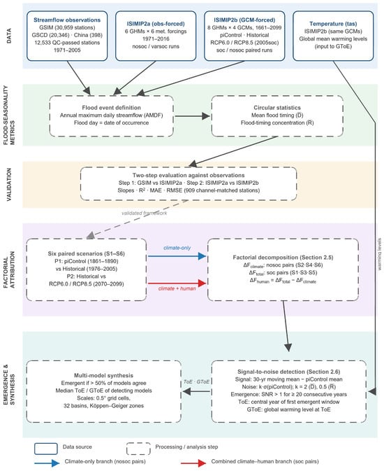
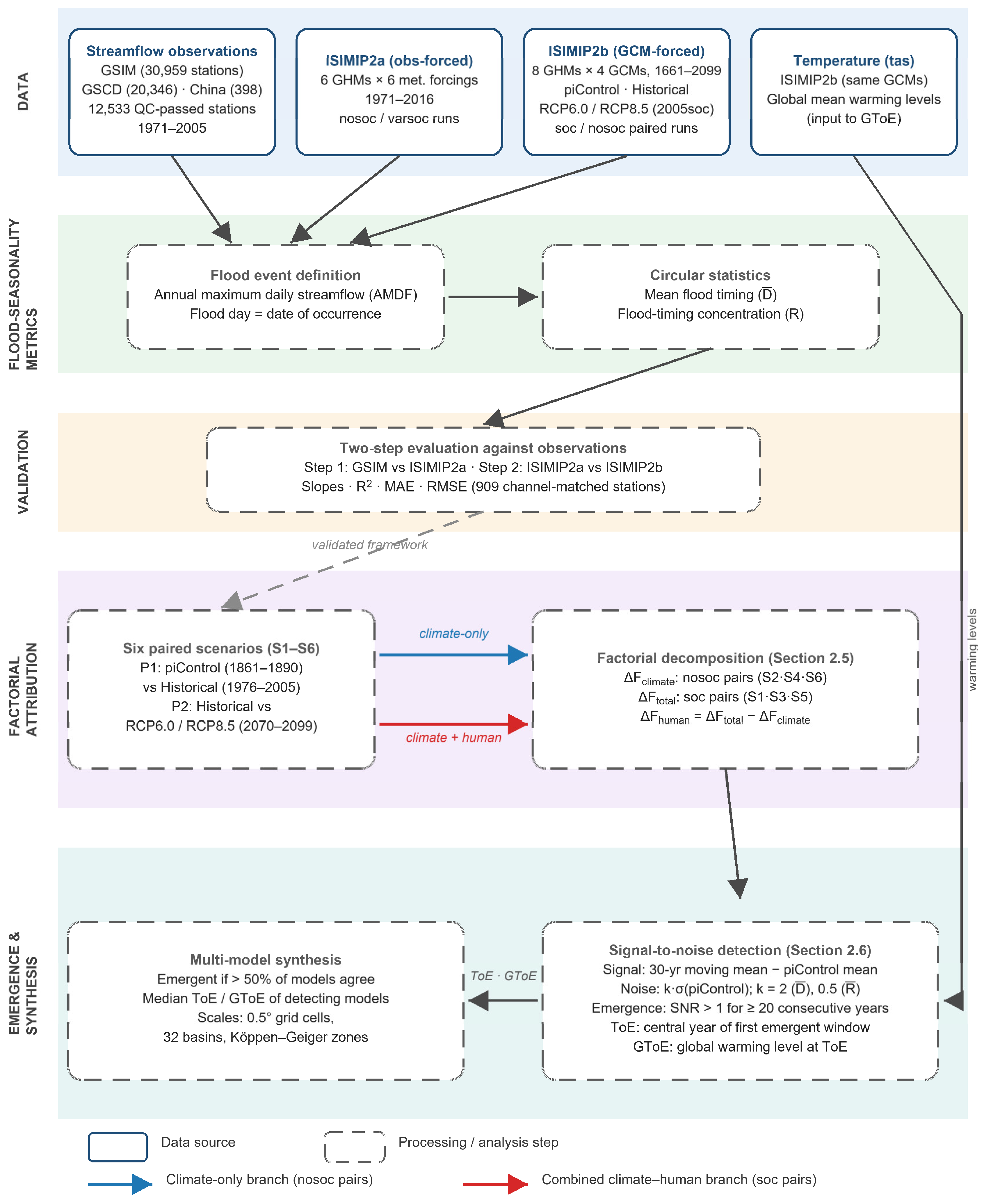
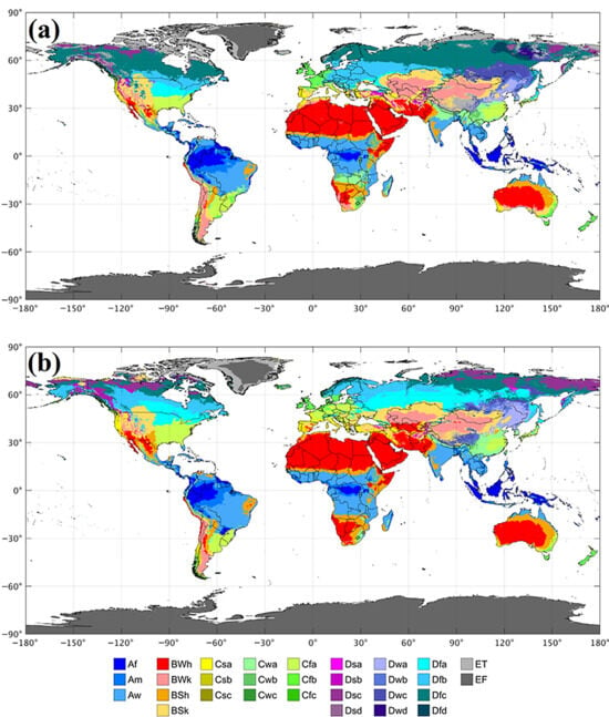
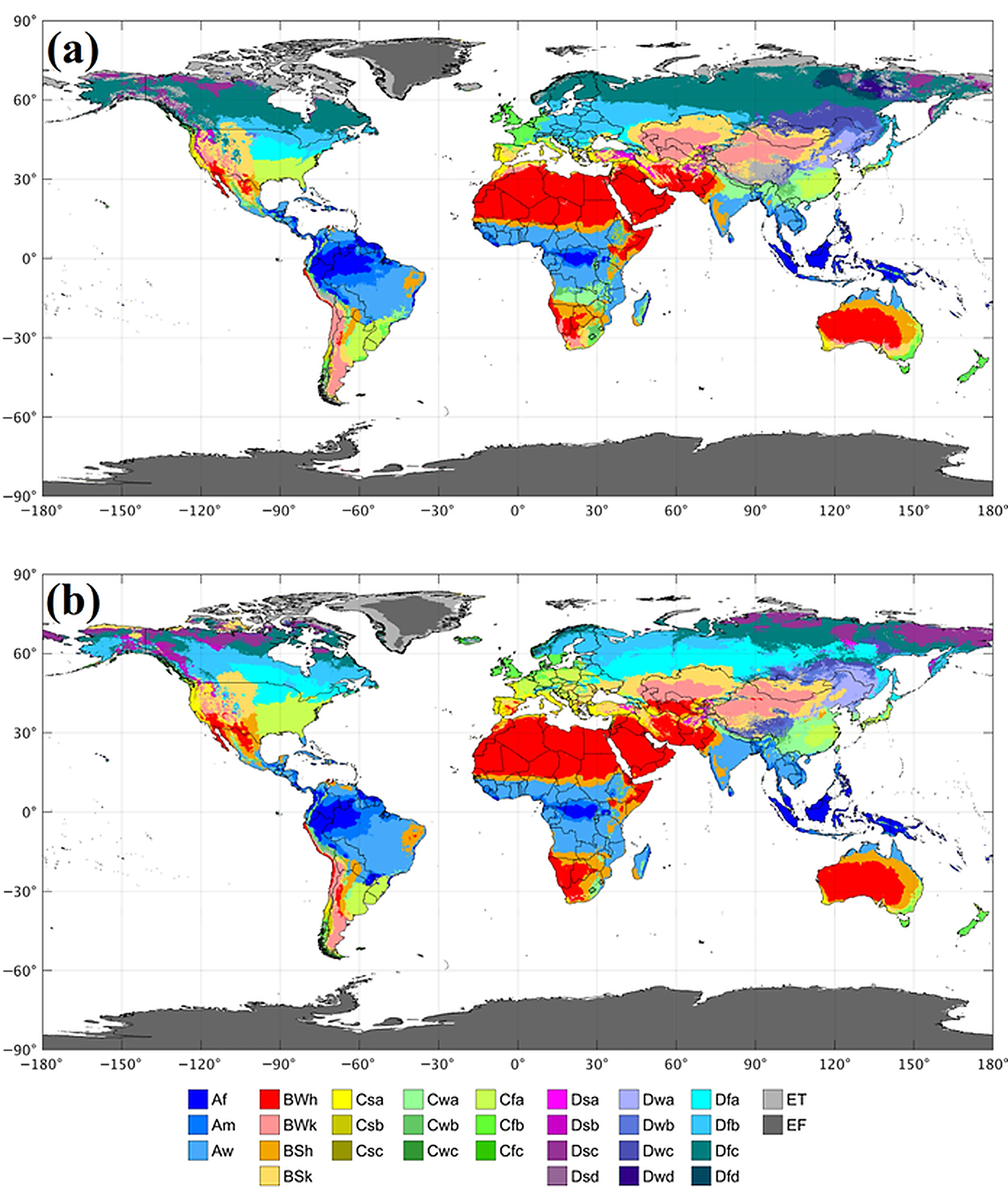
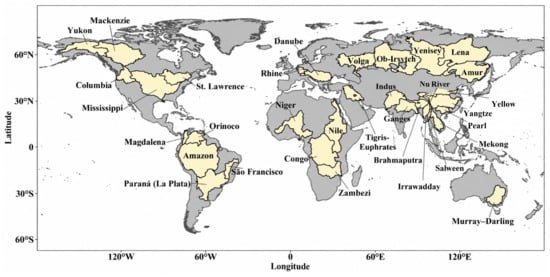
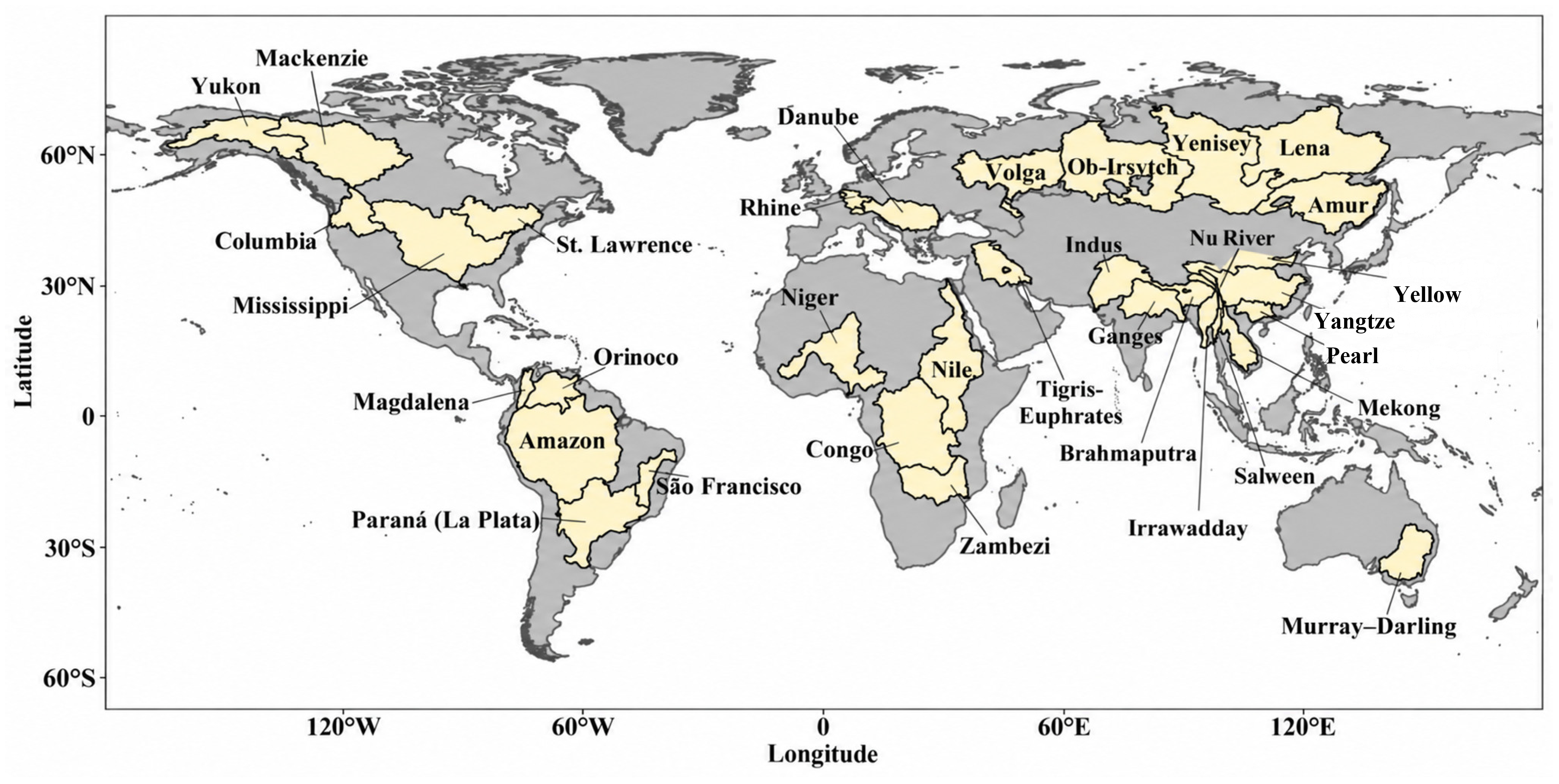
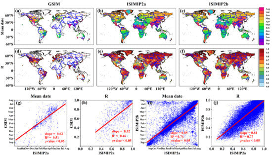
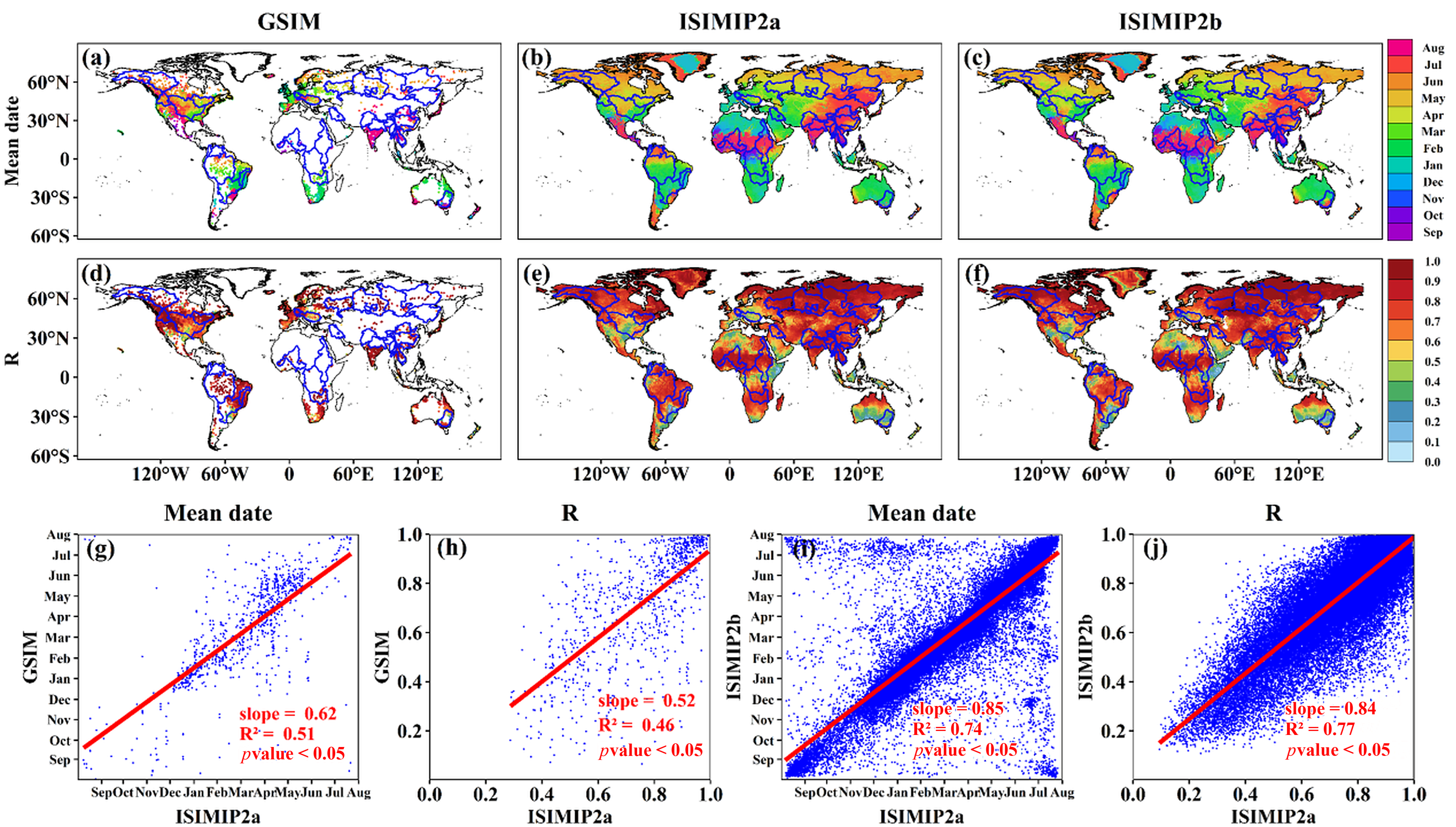
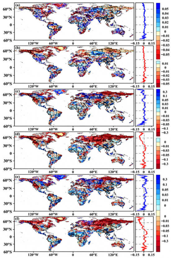
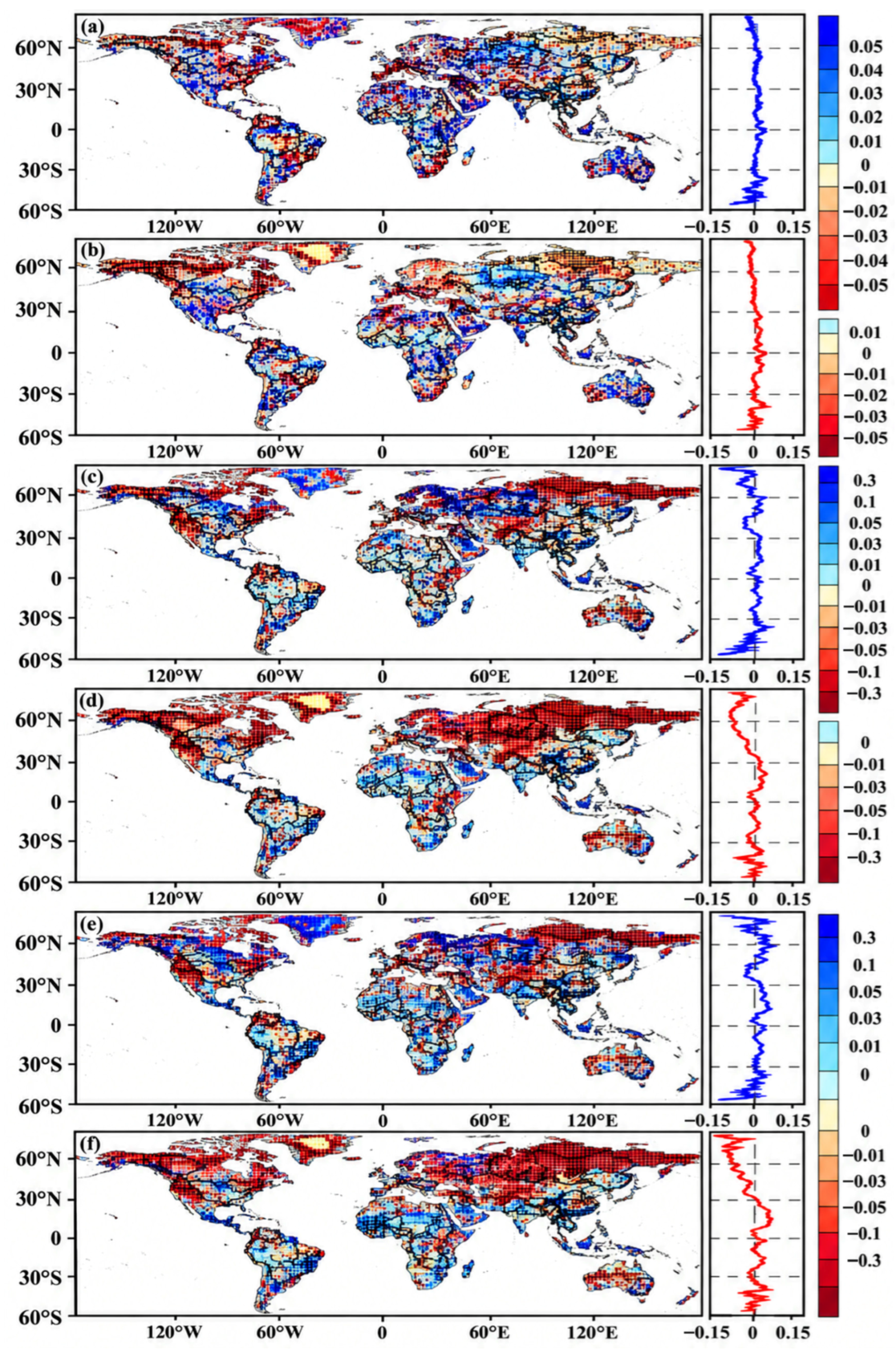
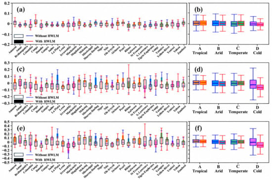
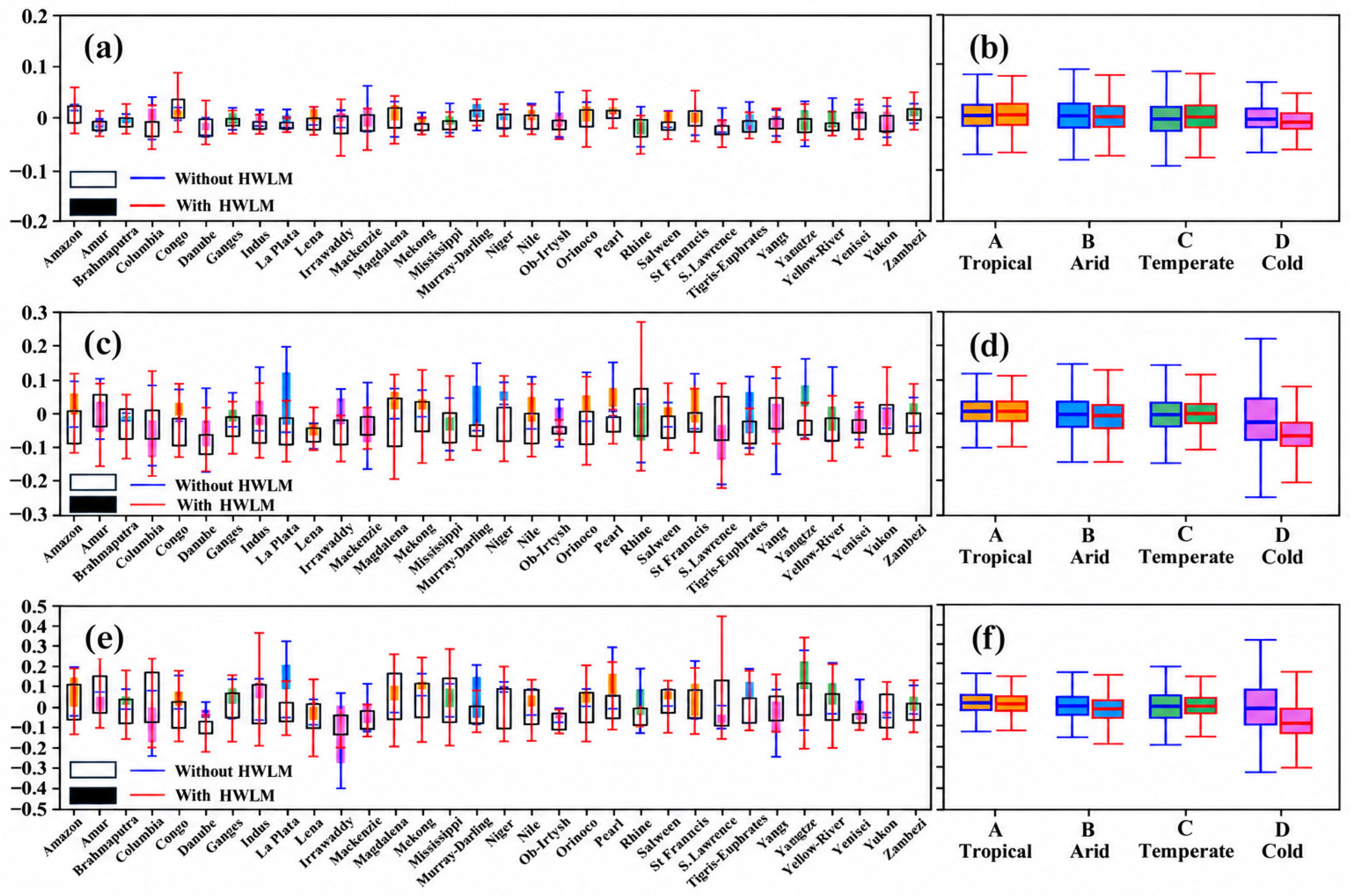
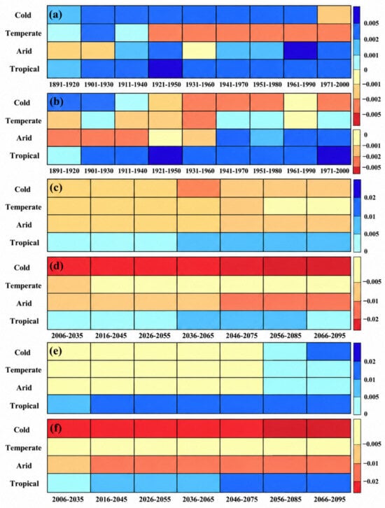
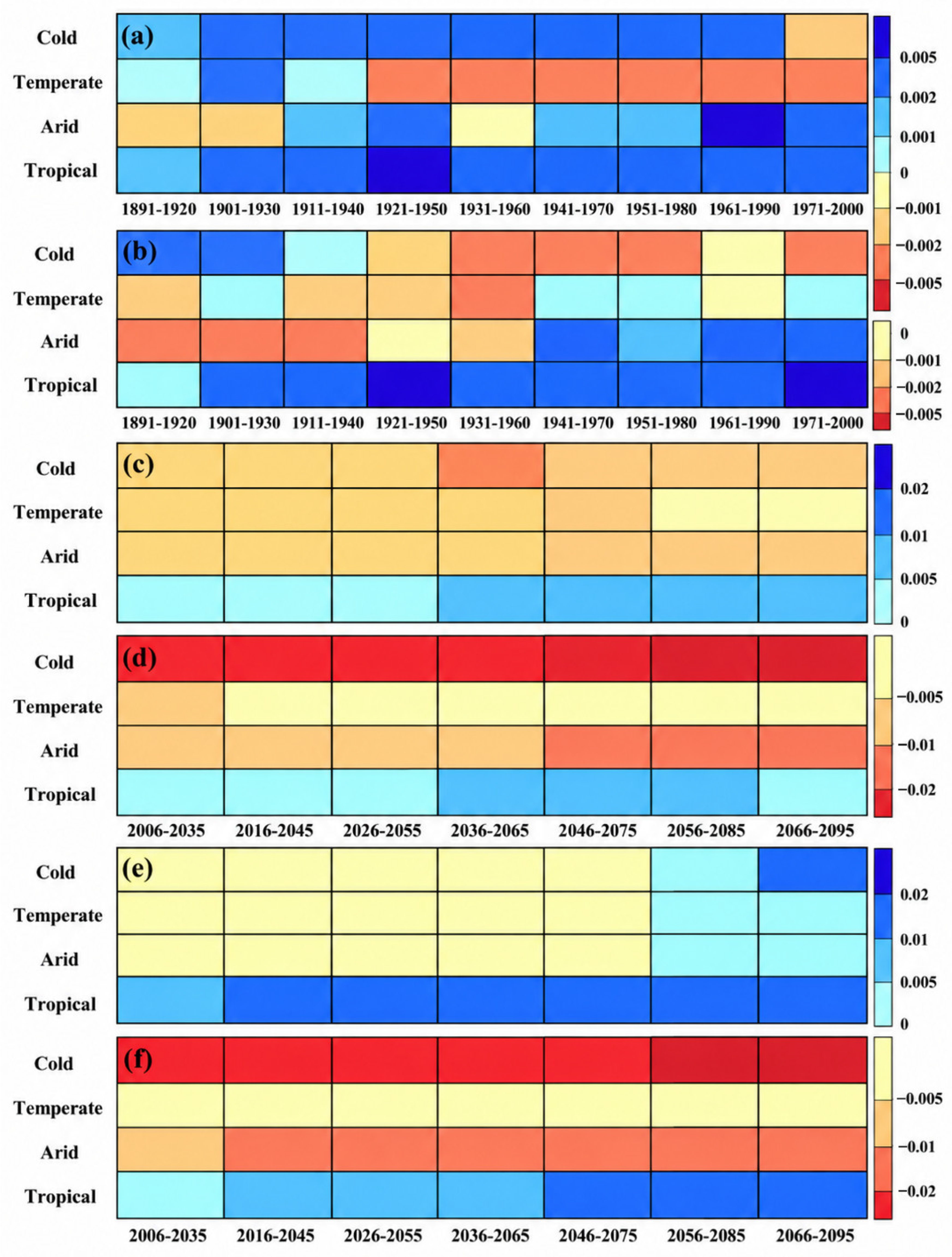
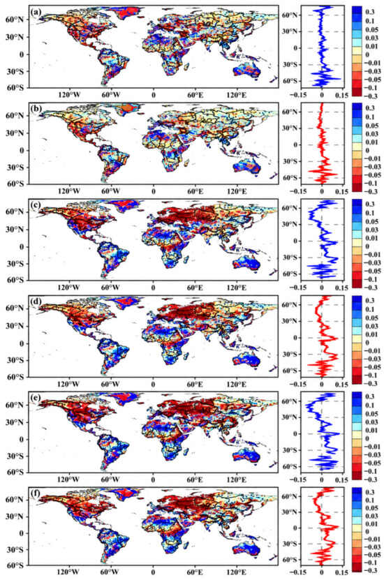
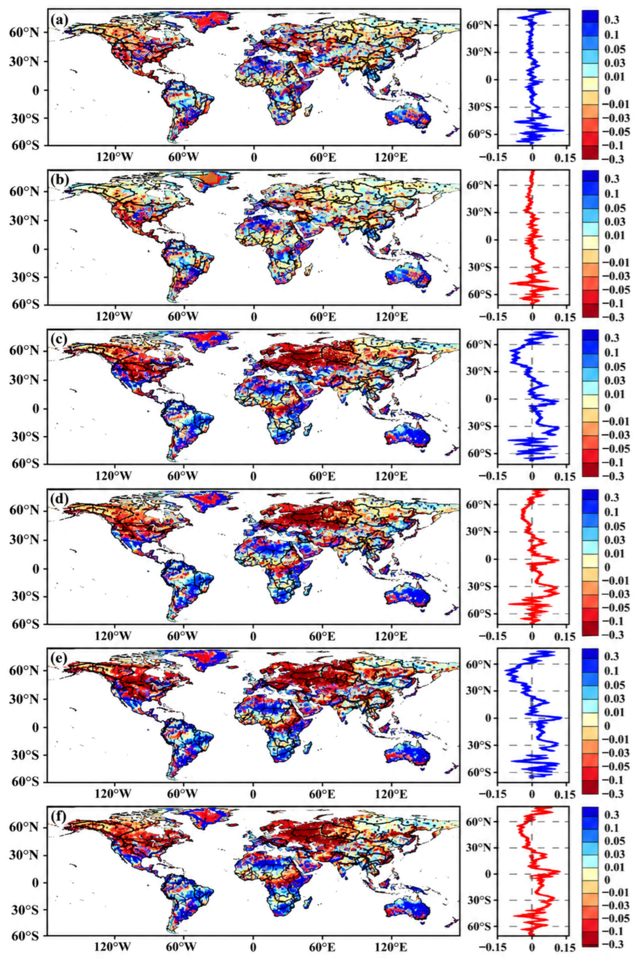
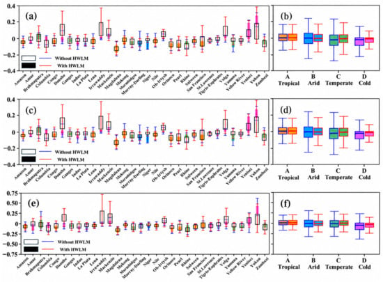
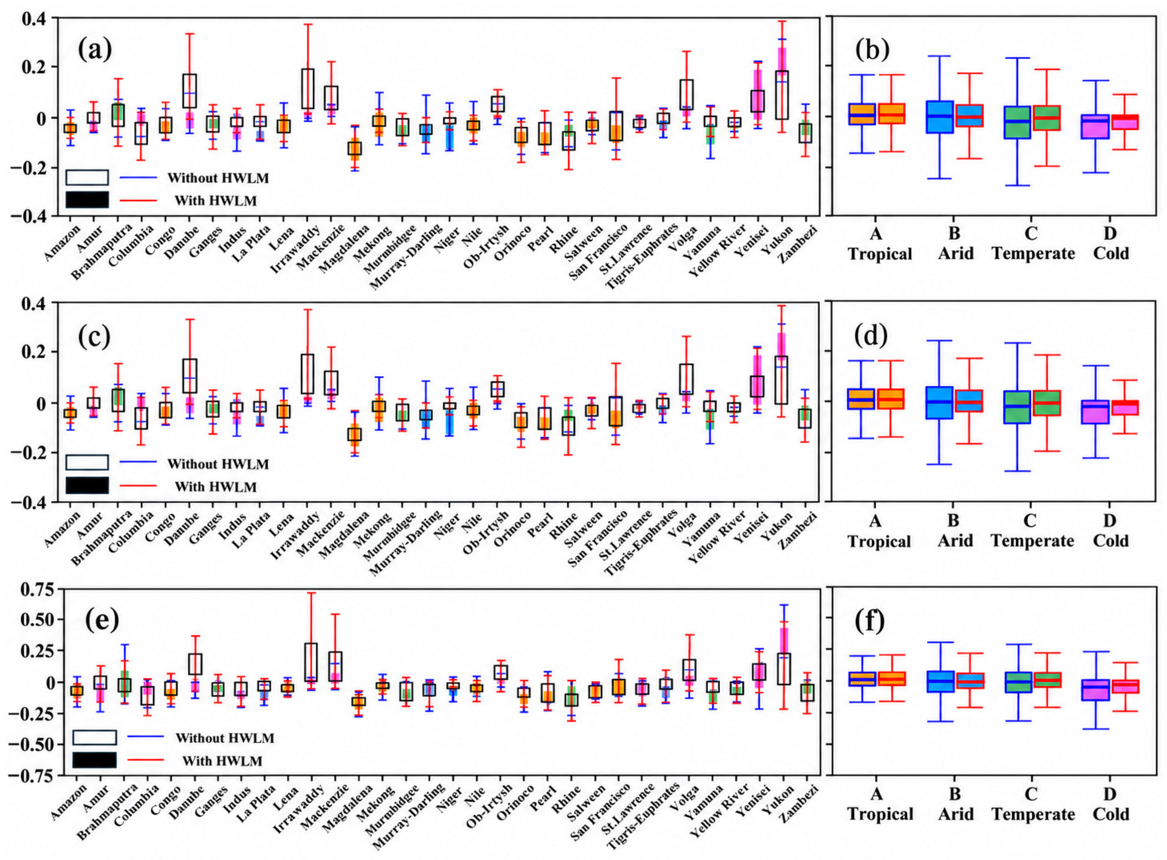
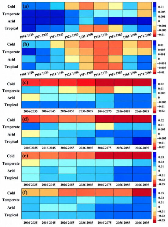
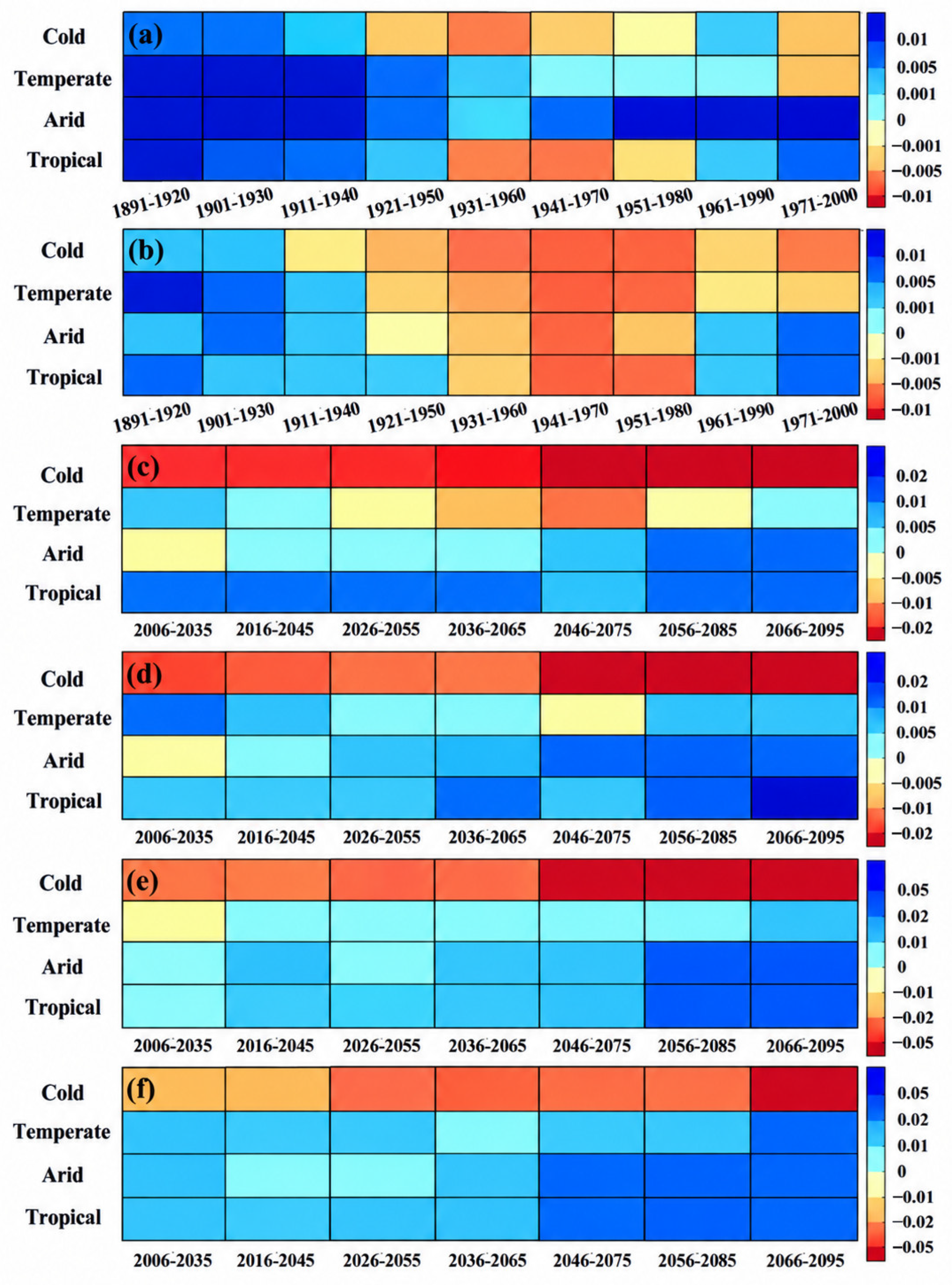
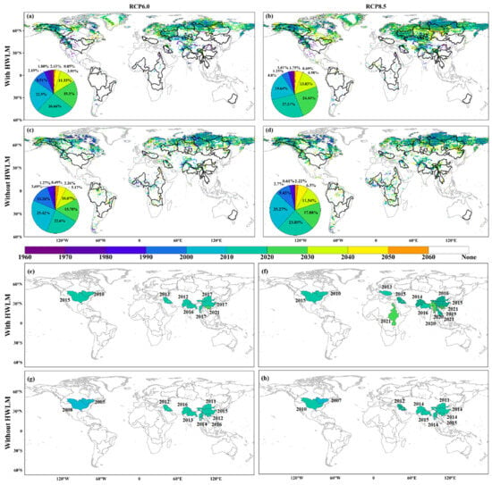
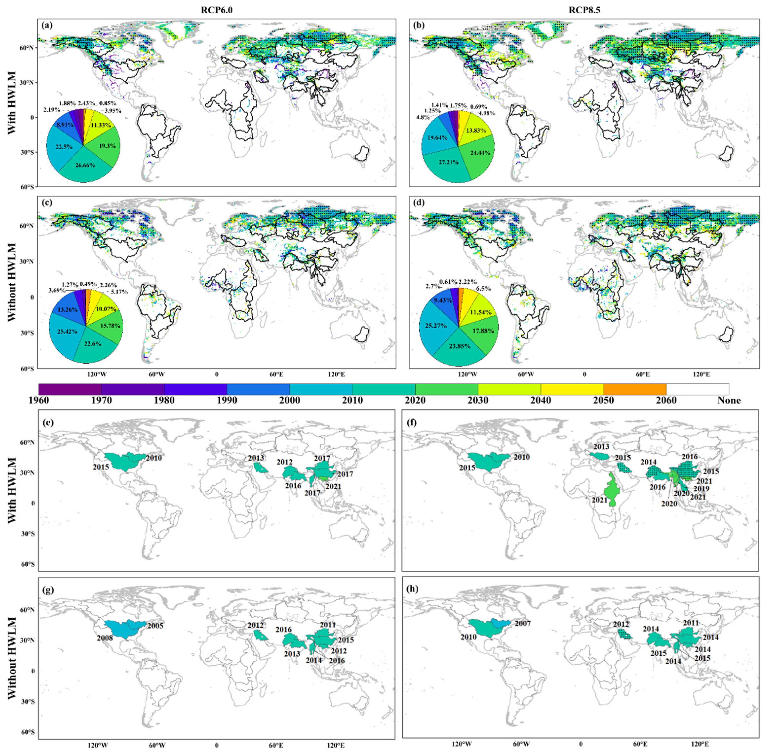
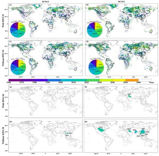
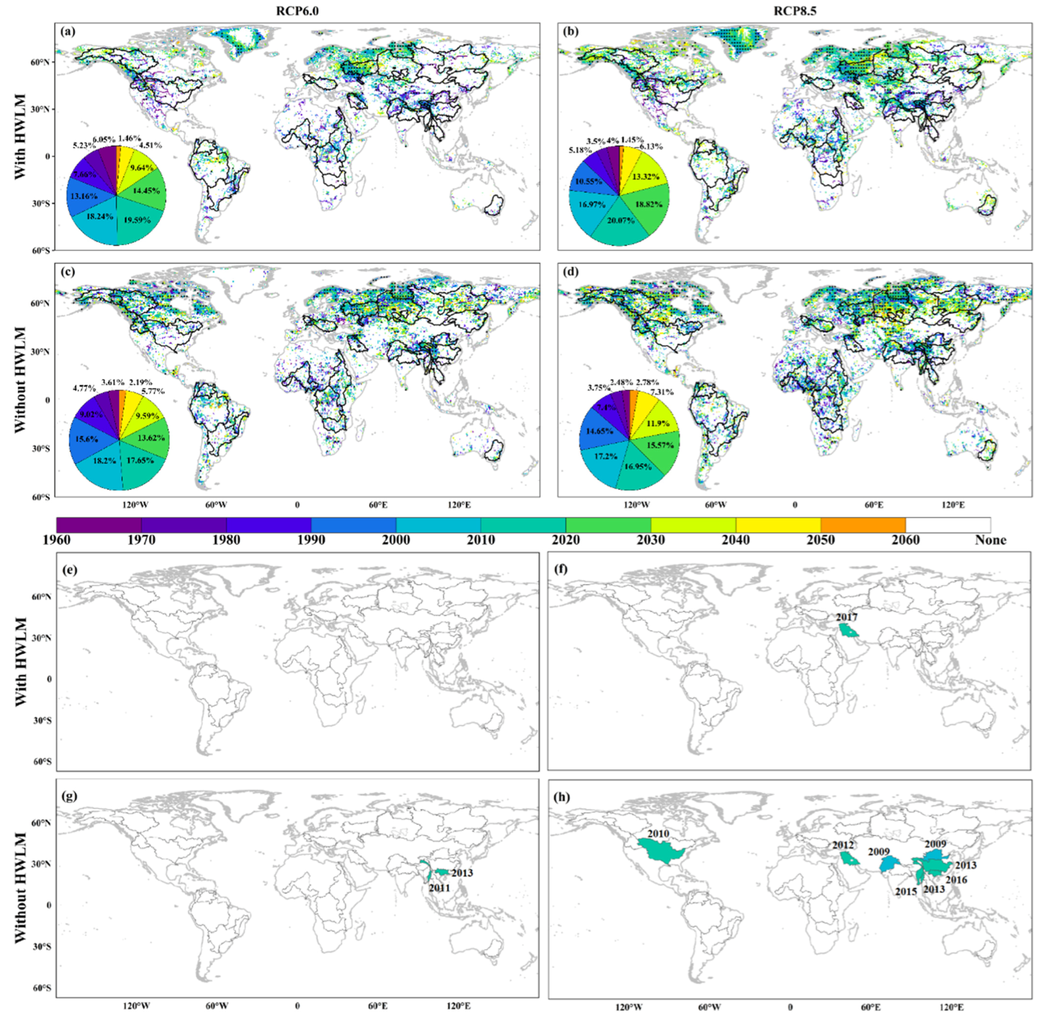
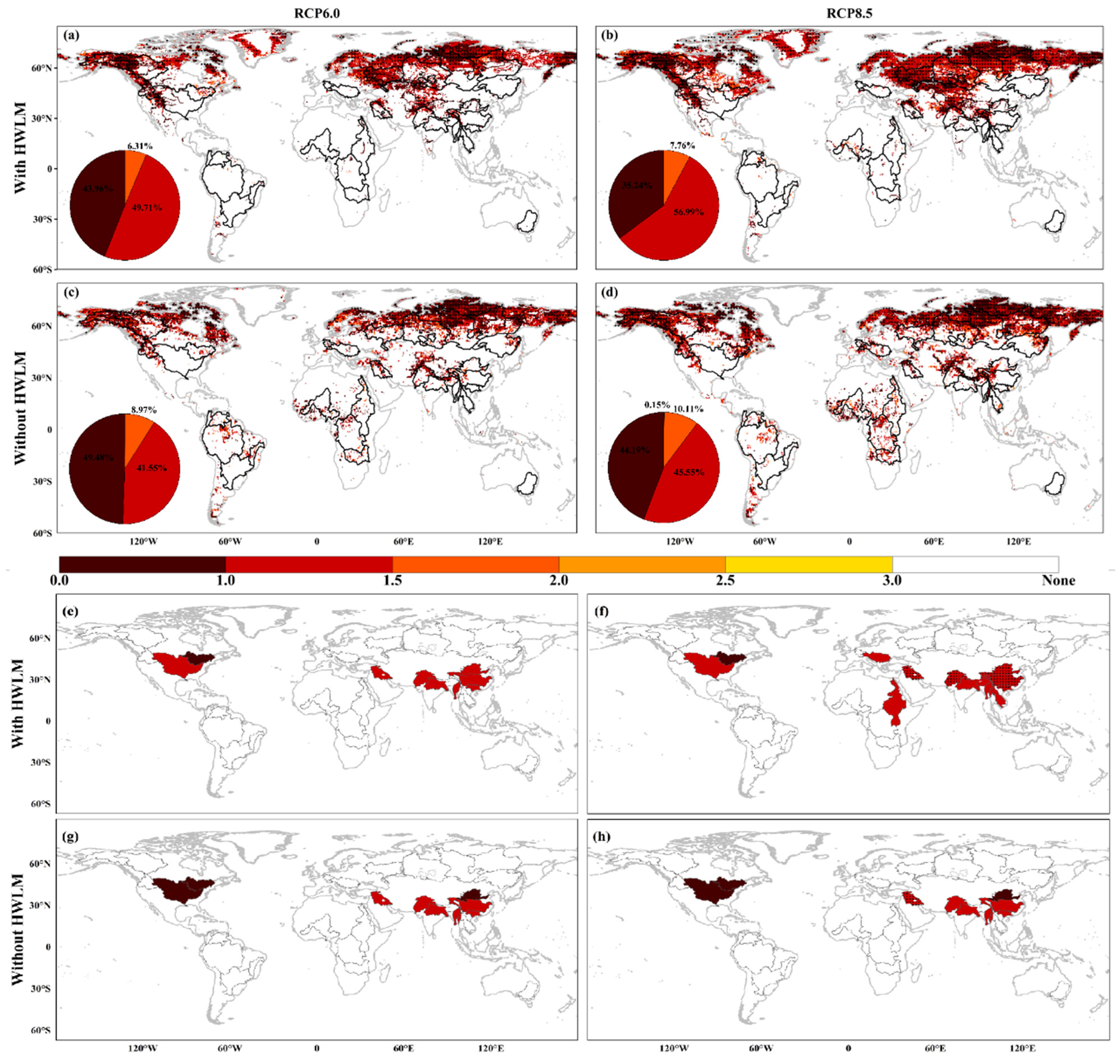
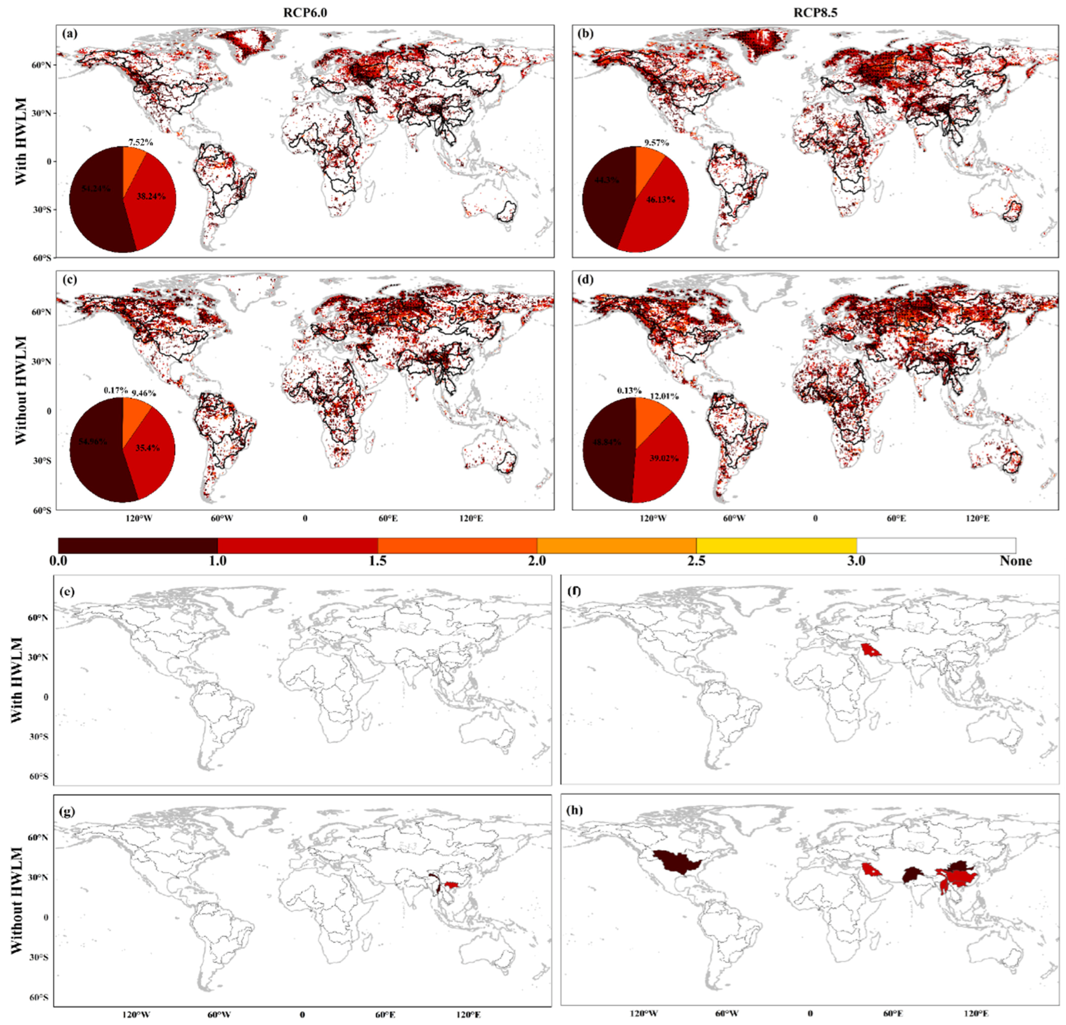
Disclaimer/Publisher’s Note: The statements, opinions and data contained in all publications are solely those of the individual author(s) and contributor(s) and not of MDPI and/or the editor(s). MDPI and/or the editor(s) disclaim responsibility for any injury to people or property resulting from any ideas, methods, instructions or products referred to in the content. |
© 2026 by the authors. Licensee MDPI, Basel, Switzerland. This article is an open access article distributed under the terms and conditions of the Creative Commons Attribution (CC BY) license.