A Nash Bi-Level Optimization Framework for Competing Cleaner Closed-Loop Supply Chains in the Power Battery Industry

Abstract

Background: Power battery closed-loop supply chains face simultaneous competition for scarce materials, subsidies, market demand, and recyclable batteries, while strategic decisions remain coupled with production, recovery, transport, inventory, and carbon-control operations. Methods: We develop a Nash-type bi-level framework for two homogeneous competing chains, in which simultaneous upper-level strategies determine conditional lower-level operating responses. Shared resources make feasibility strategy-dependent; therefore, the computational target is a finite-candidate approximate equilibrium rather than an analytically solved continuous equilibrium. Public-information-adapted benchmarks are used for finite-grid validation, algorithm and model comparison, and sensitivity analysis. Results: The proposed framework approaches the discretized reference equilibrium in the small-instance validation. In the stylized homogeneous-duopoly benchmark, the Nash-type structure provides a more suitable joint representation of competitive stability and implementation conditions than the selected Stackelberg and centralized-cooperative alternatives, while this result does not identify the competitive structure of the real battery industry. Sensitivity analysis provides directional, benchmark-specific evidence that demand and scarce-material supply are the clearest drivers, whereas policy, preference, and isolated technical parameters mainly reshape equilibrium allocation and structure. Conclusions: These findings support the framework as a conditional analytical tool for competing closed-loop supply chain planning.

1. Introduction

1.1. Research Background

The rapid expansion of new energy vehicles and the retirement of large volumes of power batteries have increased the strategic importance of battery closed-loop supply chains [1,2,3]. In the battery context, cleaner supply chain management is no longer limited to production efficiency. It also depends on battery recovery, reverse transportation, low-carbon delivery, inventory deployment, and recycled-material utilization, all of which jointly affect circularity, cost, and emissions [1,4].

At the same time, competition among major battery firms is often multidimensional rather than purely price-based. Firms may compete simultaneously for scarce raw materials and subsidy resources [5,6], as well as for market demand and end-of-life battery collection channels [7,8]. Such rivalry changes not only market outcomes but also the feasibility and consequences of production, recycling, transport, and inventory decisions. For technologically comparable firms, this interaction is difficult to represent through a fixed leader–follower structure alone, which is why strategic competition and lower-level operational execution should be analyzed jointly rather than separately. This is also the type of setting studied in generalized Nash equilibrium and shared-constraint game models [9,10].

1.2. Research Motivation

Existing studies provide a strong basis for analysing pricing, recovery, coordination, subsidy design, and battery recycling policy [1,3,5,6,7,8,11,12]. For the problem considered here, three gaps remain.

First, many studies still analyze either a single supply chain or a simplified competitive setting [5,6,8]. These formulations do not fully represent two comparable supply chains competing simultaneously for raw materials, subsidy resources, market demand, and recyclable batteries.

Second, when competition is modelled directly, Stackelberg games remain common because they can represent power asymmetry and sequential adjustment [13,14,15]. However, the present battery-duopoly setting starts from a different premise: the two supply chains are treated as structurally comparable, and no stable leader is imposed ex ante.

Third, the bi-level optimization literature has shown the importance of preserving the link between strategic choices and lower-level execution [16,17,18]. Yet lower-level responses are often aggregated, or the framework is developed for a single chain or a hierarchical game. For battery closed-loop systems, where cleaner logistics decisions directly affect both cost and emissions, a more explicit strategic–operational coupling remains necessary.

This study addresses the lack of a framework that jointly captures horizontal rivalry, lower-level operational feedback, and shared-constraint competition between comparable battery supply chains. It develops a Nash-type bi-level model and evaluates it on public-data-adapted benchmark instances, so that upper-level strategies are assessed through endogenous operational responses rather than an aggregated reaction.

1.3. Contributions of This Study

The proposed framework combines an upper-level complete-information static Nash-type game with a lower-level operational model covering production, transportation, recycling, inventory, and emission control. The lower level is evaluated through conditional lower-level optimization after $\epsilon$-constraint transformation, and the upper level is searched through a game-based evolutionary procedure to obtain finite-candidate approximate equilibria [17,18,19,20]. More precisely, the shared-resource setting induces strategy-dependent feasible correspondences at the upper level, so the computational target is a finite-candidate approximate equilibrium of a Nash-type, shared-constraint game.

The main contributions of the study are as follows.

• It formulates a Nash-type bi-level optimization framework for a homogeneous duopoly in the power battery cleaner closed-loop supply chain context, with explicit consideration of parallel competition over raw materials, subsidies, market demand, and recycling resources.
• It strengthens the strategic–operational linkage by embedding a lower-level operational model into the competitive decision structure, thereby allowing strategic choices to be evaluated through endogenous responses in production, transportation, recycling, inventory, and carbon emissions under cleaner logistics requirements.
• It adopts a problem-adapted hybrid GT-DP-NSGA-II procedure to support the computation of finite-candidate approximate equilibria for the proposed framework [17,20]. In this study, the role of the solution method is primarily to provide a credible computational basis for model evaluation rather than to claim a universally dominant algorithmic advance.

The remainder of this paper is organized as follows. Section 2 reviews the related literature. Section 3 presents the methods. Section 4 reports the main results. Section 5 discusses the findings. Section 6 concludes the paper and outlines limitations and future research directions.

2. Literature Review

2.1. Sustainable Closed-Loop Supply Chain Optimization

Sustainable closed-loop supply chain research has moved from network design and cost minimization toward more integrated analyses of recovery coordination, pricing, environmental regulation, remanufacturing, and carbon performance [4,11,12,21]. In battery-related settings, these issues are especially salient because raw-material criticality, recycling technology, and carbon mitigation are strongly interconnected [1,2,3,6,8]. Existing studies have examined battery recycling, subsidy design, information sharing, social responsibility, and technology selection [6,7,8]. However, much of this literature still focuses on a single supply chain or on a competitive structure that is simplified relative to the present battery setting. For the present study, the main implication is that a meaningful cleaner supply chain model needs to represent production, recycling, logistics, and environmental performance jointly while moving beyond isolated single-chain optimization.

2.2. Competition and Game-Theoretic Modelling in Supply Chains

Game-theoretic modelling has long been used to analyze competition and coordination in supply chains, including price competition, quantity competition, and Stackelberg structures with explicit leader–follower roles [13,14,22]. These models have generated useful insights into pricing, environmental investment, channel coordination, subsidy allocation, and recovery competition [5,13,14]. However, in settings involving technologically comparable firms, a stable leader is not always evident [15]. This is particularly relevant for power battery closed-loop systems, where firms may compete simultaneously for materials, subsidies, market demand, and recycling sources [6,7]. The literature therefore leaves open whether a simultaneous Nash-type structure with shared constraints can better represent such parallel rivalry.

2.3. Bi-Level Optimization and Strategic–Operational Coupling

Bi-level optimization is useful when strategic decisions influence, and are influenced by, lower-level operational responses [16,17,18]. In sustainable supply chains, this linkage matters because pricing, resource allocation, and sustainability commitments change the feasible region and cost structure of production, transportation, inventory, and recovery decisions [2,17]. For closed-loop power battery systems, where these lower-level decisions jointly affect both cost and emissions [1,2], highly aggregated operational responses may weaken model realism. A remaining need is therefore a framework that combines horizontal strategic competition with explicit cleaner-logistics execution within each supply chain.

2.4. Assessment of the Literature

Table 1 summarizes representative studies from the perspectives of research object, competition structure, core decision focus, bi-level modelling, lower-level solution treatment, power battery scenario, strategic–operational coupling, and solution method. The comparison highlights the gap addressed here: limited work combines homogeneous-duopoly competition, battery closed-loop context, and explicit strategic–operational coupling under cleaner logistics requirements. To improve reproducibility of the qualitative assessment, ✓ denotes explicit coverage, × denotes absence, and P denotes partial coverage. The Weak/Medium/Strong labels are used only for the strategic–operational coupling column and are defined operationally in the note below Table 1.

Table 1. Comparison of representative literature on sustainable closed-loop supply chain competition and bi-level solution.

The Literature	Research Object	Competition Structure	Core Decision	Bi- Level	LL Solution	Power Battery	Strategic– Operational Coupling	Solution Method	Main Limitation
Wang et al. [5]	Mixed CLSC	Product + recycling competition	Pricing, recycling	×	×	×	Weak	Game analysis	Non-battery setting; no explicit execution layer.
Xiao et al. [6]	Competitive EV battery CLSC	Competitive game	Information sharing, subsidy, recycling	×	×	✓	Weak	Game analysis	Policy-oriented; operational response simplified.
Hu and Hou [8]	EV battery CLSC	Hybrid competition/ cooperation	CSR, cascade use, recycling	×	×	✓	Weak	Game model	No explicit bi-level execution under parallel duopoly.
Pakseresht et al. [13]	Sustainable product family chain	Stackelberg	Sustainable design, allocation, pricing	✓	P	×	Strong	Bi-level optimization	Strong leader–follower setting; not tailored to homogeneous parallel competition.
Abbasi et al. [15]	Duopoly remanufacturing	Stackelberg–Nash	Entry, pricing	P	×	×	Medium	Combinatorial game framework	Focus on remanufacturing barriers; limited closed-loop network detail.
Setak et al. [17]	Competitive reliable SC	Competitive bi-level	Allocation, assignment, reliability	✓	✓	×	Strong	Exact methods + GA	Not sustainability-focused; non-battery context.
Konak et al. [23]	Server assignment under attack	Competitive information game	Assignment	×	×	×	Weak	GTGA evolution	Algorithmically relevant, not a CLSC operations study.
Tajik et al. [3]	Battery CLSC network design	Limited duopoly emphasis	Network design, digitalization	✓/P	P	✓	Strong	Optimization model	Battery context is clear; competitive game is less explicit.
Scheller et al. [2]	Li-ion battery CLSC planning	Weak competition/case analysis	Network structure, production planning	P	✓	✓	Strong	Case optimization	No explicit duopoly game structure.
This work	Battery CLSC duopoly	Static Nash	Resources, subsidy, pricing, recycling, operations	✓	✓	✓	Strong	Hybrid conditional LL + evolutionary search	Battery-duopoly specific.

Note: “LL solution” indicates whether the study includes an explicit lower-level solution treatment; “CLSC” denotes closed-loop supply chain; “P” denotes partial or partially satisfied. ✓ denotes explicit coverage and × denotes absence. For strategic–operational coupling, Weak means that operational execution is absent, qualitative, or simplified into aggregate parameters; Medium means that operational factors enter the model or experiment but are not solved as an explicit linked response to strategic decisions; Strong means that operational decisions are explicitly optimized and fed back to strategic objectives, feasibility, or equilibrium evaluation. These labels are coding rules for this review table rather than normative quality rankings.

The preceding review suggests that the literature has generated substantial knowledge in three related areas: sustainable closed-loop supply chain optimization, game-theoretic modelling of supply chain competition, and bi-level optimization with operational feedback. However, these strands have not yet been sufficiently integrated for the specific setting addressed in this paper.

More specifically, a gap remains in the modelling of homogeneous duopolistic power battery supply chains that compete in parallel for multiple scarce resources while also facing endogenous operational and environmental consequences. Existing studies either emphasize sustainable closed-loop operations without adequately modelling horizontal rivalry, or analyze competition under simplified strategic structures that do not fully preserve operational feedback. In addition, although hybrid computational methods are increasingly used in complex bi-level problems, their main relevance in the present context lies in enabling credible evaluation of the proposed model rather than constituting the primary research novelty.

Against this background, this study positions its contribution at the intersection of the three streams reviewed above. Its methodological novelty lies in the explicit combination of a shared-constraint competitive structure, conditional lower-level response evaluation, and finite-candidate approximate-equilibrium screening, drawing on the generalized Nash perspective that player feasibility may depend on rival decisions [9,10]. Its application novelty lies in formulating these ideas for competing sustainable closed-loop supply chains in the power battery industry, with explicit attention to strategic–operational coupling under resource, subsidy, demand, and recycling constraints. In this sense, the paper aims to extend the literature not by claiming a universally dominant algorithmic approach, but by providing a more suitable problem formulation for the competitive setting considered and by supporting that formulation with a computationally credible solution process.

3. Materials and Methods

3.1. Problem Setting

This study considers two competing cleaner closed-loop supply chains in the power battery industry. Each chain includes a focal battery enterprise and its production, recovery, transportation, and inventory network. The two chains compete not only in product sales but also in scarce materials, subsidy resources, and recoverable end-of-life batteries.

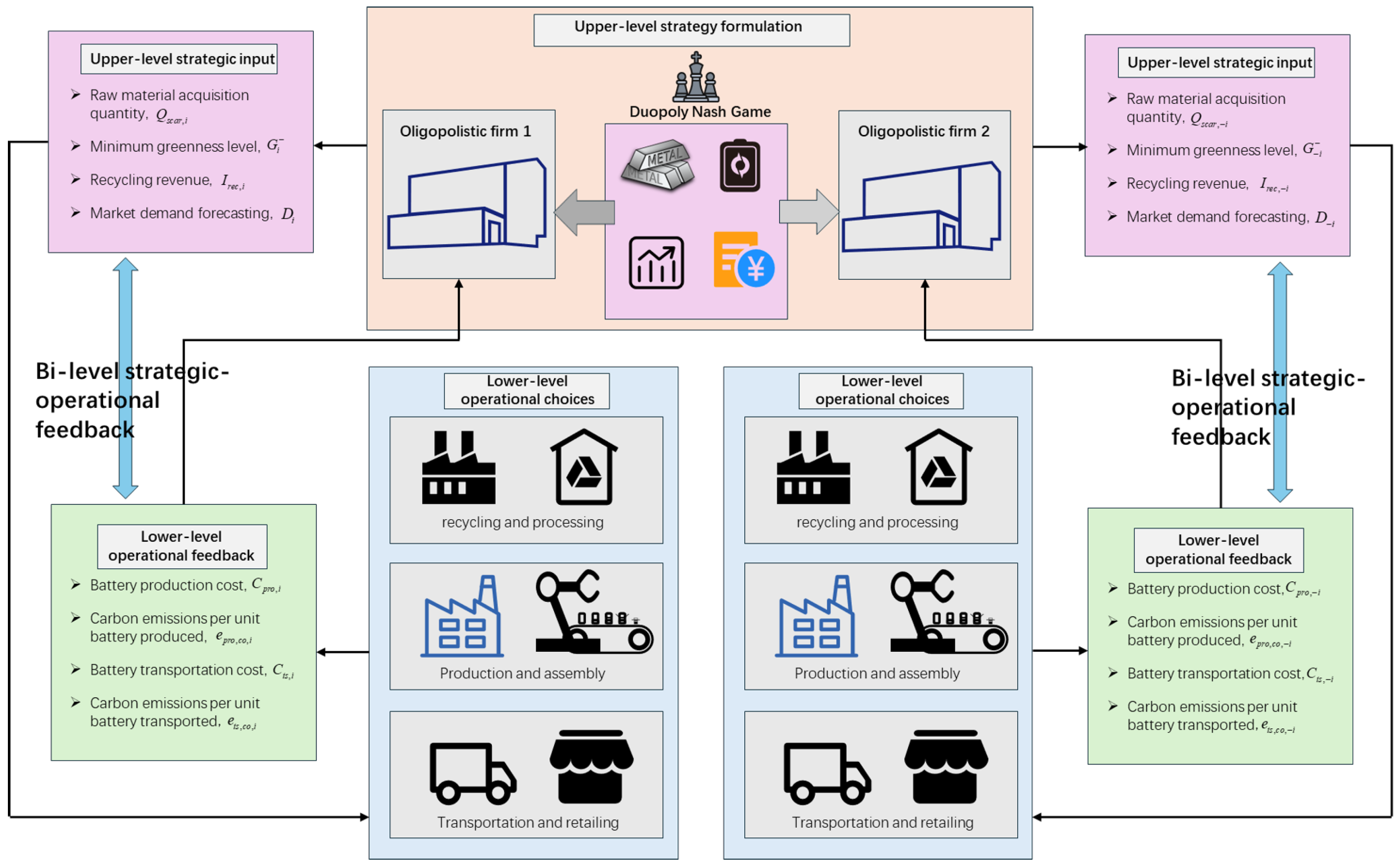
Figure 1 depicts the model itself rather than an alternative game structure: the two supply chains interact through a simultaneous duopoly Nash game at the upper level, while each chain contains a bidirectional link between upper-level strategic inputs and lower-level operational feedback.

Figure 1. Conceptual structure of the Nash-type bi-level strategic–operational coupling.

At the strategic layer, each supply chain chooses raw-material bidding intensity, sustainability commitment, output, price, and recycling effort. At the operational layer, these strategic decisions are translated into feasible production, transportation, recycling, and inventory plans under capacity, material-balance, and carbon constraints.

The modelling question is whether, for relatively homogeneous competing battery supply chains, a simultaneous complete-information Nash-type structure is more suitable than alternative upper-level structures within the stylized benchmark once operational feedback is retained explicitly.

3.2. Model Assumptions

The following assumptions define the model scope.

• The market consists of two comparable power battery supply chains competing in parallel. Neither supply chain is assumed a priori to possess a stable leadership position over the other at the upper strategic level.
• The upper-level interaction is modelled as a complete-information static game. Each supply chain is assumed to know the relevant structure of the problem, including resource limits, demand environment, and the form of the rival’s strategic decision space.
• Competition takes place simultaneously with respect to strategic variables, including raw-material acquisition intensity, sustainability commitment, planned output commitment, pricing, and recycling effort. The resulting allocations of scarce raw materials, subsidy resources, market demand, and recoverable batteries are endogenous to the competitive decisions of both firms.
• The two supply chains are treated as homogeneous in the sense that they operate in the same industry context and face comparable categories of decisions and constraints. Homogeneity here does not imply identical numerical parameters, but rather a symmetric modelling structure.
• The lower-level model represents the internal operational response of each supply chain after upper-level decisions are specified. It does not choose the strategic output commitment itself; rather, it allocates the committed output across production lines, material options, recycling technologies, transport modes, and inventories under feasibility and carbon constraints.
• Lower-level operational optimization is assumed to be rational and feasible whenever a candidate upper-level decision is admissible. For a fixed upper-level strategy pair, the lower-level multi-objective operational model is transformed through the $\epsilon$-constraint method and optimized by CPLEX as a mathematical-programming subproblem. The resulting output is referred to as a conditional lower-level response: CPLEX optimality applies to the fixed subproblem and does not imply a closed-form or global solution of the full continuous game.
• Demand, subsidy resources, scarce materials, and recoverable battery quantities are treated as deterministic within a planning period. Dynamic adjustment, incomplete information, and stochastic disturbances are not considered in the present model.
• The model focuses on a single planning stage under static competition. Intertemporal learning, repeated interaction, reputation effects, and long-horizon contract dynamics are beyond the scope of this study.

3.3. Decision Logic and Modelling Scope

Three terminology levels are used in this study. First, the modelling framework is a Nash-type bi-level model: two homogeneous supply chains choose strategic variables simultaneously, and each strategy is evaluated through its conditional lower-level operational response. Second, the continuous-space conceptual reference is a shared-constraint generalized Nash equilibrium benchmark, because shared resources make each chain’s feasible set dependent on the rival’s strategy. Third, the actual computational target is a finite-candidate approximate equilibrium obtained from the evaluated candidate set and screened by objective quality and local unilateral-deviation pressure. Unless explicitly stated otherwise, all reported equilibria in the computational sections refer to this finite-candidate approximate-equilibrium concept rather than to an analytically solved continuous-space equilibrium.

Each supply chain selects an upper-level strategy vector covering material acquisition, sustainability commitment, output, price, and recycling effort. Given a strategy pair $s=(s_1,s_2)$, government, market, material, and recycling constraints determine the strategy-dependent feasible set, while the lower-level response of chain i, denoted by $R_i(s_i,s_{-i})$, allocates production, logistics, recycling, and inventory resources. The resulting profit and sustainability-performance outcomes are fed back to the upper level, and reported solutions are finite-candidate approximate equilibria.

3.4. Mathematical Models

3.4.1. Notation

The main notation is summarized in Table 2. Unless otherwise stated, subscript i denotes the supply chain, while k, s, e, t, m, and l denote production lines, production schemes, material options, recycling technologies, transfer centres, and transport modes, respectively. Superscripts such as “pro”, “log”, “mat”, and “rec” identify production, logistics, material, and recycling-related quantities.

Table 2. Main notation used in the bi-level model.

Category	Symbol	Description
Strategic variables	${\alpha }_i$	Raw-material bidding coefficient of supply chain i
	${\gamma }_i$	Minimum sustainability commitment of supply chain i
	$q_i$	Strategic planned output commitment of supply chain i
	$p_i$	Selling price of supply chain i
	$r_i$	Recycling effort coefficient of supply chain i
	${\pi }_i$	Total profit of supply chain i
	$G_i$	Realized sustainability-performance level of supply chain i
	$S_i$	Realized sales volume of supply chain i
	$D_i$	Market demand allocated to supply chain i
	$B_i$	Sustainability subsidy obtained by supply chain i
Operational response variables	$X_{k,s,e,i}$	Production quantity on line k under scheme s and material option e in supply chain i
	$Y_{t,i}$	Processing quantity of recycling technology t in supply chain i
	$Z_{k,m,l,i}$	Transport quantity from line k via transfer centre m using mode l in supply chain i
	$I_i^{\mathrm{mat}}$	Raw-material inventory of supply chain i
	$I_i^{\mathrm{pro}}$	Finished-goods inventory of supply chain i
	$R_{\mathrm{mat},i}$	Regenerated raw-material quantity of supply chain i
	$C_i^{\mathrm{oper}}$	Total operating cost of supply chain i
	$E_i^{\mathrm{total}}$	Total carbon emissions of supply chain i
	$E_i^{\mathrm{pro}},E_i^{\log }$	Production- and logistics-stage carbon emissions of supply chain i
Endogenous allocation quantities	$Q_{\mathrm{scar},i}$	Acquired scarce raw-material quantity of supply chain i
	$Q_{\mathrm{rec},i}$	Recovered end-of-life battery quantity of supply chain i
	$C_i^{\mathrm{pur}}$	Procurement expenditure on scarce raw materials of supply chain i
	$C_i^{\mathrm{rec}}$	Upper-level recycling investment expenditure of supply chain i
	$I_i^{\mathrm{rec}}$	Upper-level recycling investment decision of supply chain i
	$C_i^{\mathrm{LL}}$	Aggregated conditional lower-level operating cost of supply chain i
	$C_i^{\mathrm{pro}},C_i^{\log },C_i^{\mathrm{rec},\mathrm{op}}$	Lower-level production, logistics, and recovery-operation costs of supply chain i
	$C_i^{\mathrm{sto}}$	Inventory/storage cost of supply chain i
	$C_i^{\mathrm{pen}}$	Environmental penalty cost of supply chain i
Parameters and coefficients	${\overline{Q}}_{\mathrm{scar}}$	Total market supply of scarce raw materials
	${\overline{Q}}_{\mathrm{rec}}$	Total recoverable quantity of end-of-life batteries
	$\overline{B}$	Total government sustainability subsidy budget
	$\overline{D}$	Upper bound of total market demand
	${\overline{F}}_i$	Available capital of supply chain i
	${\overline{E}}_i$	Benchmark carbon-emission quantity for supply chain i
	$\mathsf{\Omega }$	Raw-material consumption coefficient per unit product
	${\eta }_t$	Material conversion rate of recycling technology t
	${\rho }_e$	Regenerated-material usage ratio under material option e
	${\delta }_{k,s}$	Compatibility parameter between production line k and scheme s
	${\sigma }_{m,l}$	Compatibility parameter between transfer centre m and transport mode l
	${\theta }_m$	Demand allocation coefficient associated with transfer centre m
	$\alpha ,\beta ,\gamma$	Elasticity coefficients in the demand allocation function
	$c_i^{\mathrm{base}}$	Base unit cost of scarce raw material for supply chain i
	${\kappa }_i$	Procurement-cost sensitivity to the raw-material bidding coefficient of supply chain i
	${\overline{P}}_k,{\overline{T}}_t,{\overline{V}}_l,$ $M,\epsilon$	Capacity limits of production, recycling, transport, the large-M constant, and the lower-level emission bound

3.4.2. Upper-Level Nash-Type Shared-Constraint Model

At the upper level, the strategic interaction between the two competing supply chains is represented as a complete-information static Nash-type game. Each supply chain simultaneously chooses its strategic variables with the dual objective of improving profit and sustainability performance. The game structure is

$$N=\{1,2\},S=S_1\times S_2,s=(s_1,s_2)\in S$$

(1)

with strategy set

$$S_i=\left\{({\alpha }_i,{\gamma }_i,q_i,p_i,r_i)\mid {\alpha }_i,{\gamma }_i,q_i,p_i,r_i\ge 0\right\}$$

(2)

Because market demand, scarce materials, subsidy resources, and recoverable batteries are allocated jointly across the two supply chains, not every element of $S_i$ remains admissible after the rival’s strategy is fixed. Let ${\mathcal{F}}_i\left(s_{-i}\right)\subseteq S_i$ denote the induced feasible correspondence of supply chain i, including the upper-level shared constraints and the feasibility of its conditional lower-level response. The implemented game is therefore represented by the strategy-dependent feasible profile $s_i\in {\mathcal{F}}_i\left(s_{-i}\right)$. This gives the continuous conceptual model a shared-constraint generalized Nash reference while the computational analysis remains based on finite-candidate approximate equilibria [9,10]. Here, $q_i$ is an upper-level planned output commitment used in market competition and resource allocation. It is different from the lower-level production-allocation variables $X_{k,s,e,i}$, which determine how the committed quantity is implemented across specific production lines, schemes, and material options. The upper-level bi-objective structure for supply chain i is

$$\max {\pi }_i(s_i,s_{-i}),\max G_i(s_i,s_{-i})$$

(3)

For compactness, the upper-level profit of supply chain i is written as

$$\begin{array}{c}{\pi }_i=p_i{S}_i+B_i-C_i^{\mathrm{pur}}-C_i^{\mathrm{rec}}\\ -C_i^{\mathrm{LL}}-C_i^{\mathrm{pen}}.\end{array}$$

(4)

The main intermediate quantities are

$$Q_{\mathrm{scar},i}={\displaystyle \frac{{\alpha }_i}{{\alpha }_i+{\alpha }_{-i}}}{\overline{Q}}_{\mathrm{scar}}$$

(5)

$$B_i={\displaystyle \frac{{\gamma }_i{q}_i}{{\gamma }_i{q}_i+{\gamma }_{-i}{q}_{-i}}}\overline{B}$$

(6)

$$\begin{array}{c}{D}_i={\displaystyle \frac{q_i^{\alpha }{p}_i^{-\beta }{\gamma }_i^{\gamma }}{q_i^{\alpha }{p}_i^{-\beta }{\gamma }_i^{\gamma }+q_{-i}^{\alpha }{p}_{-i}^{-\beta }{\gamma }_{-i}^{\gamma }}}\\ \times \overline{D}\end{array}$$

(7)

Here, ${\gamma }_i$ is the upper-level sustainability commitment used in the market-attractiveness function, whereas $G_i$ is the realized sustainability-performance level computed after the conditional lower-level response. This distinction prevents a circular dependence of demand allocation on the lower-level emission outcome.

$$G_i={\displaystyle \frac{{\overline{E}}_i}{E_i^{\mathrm{pro}}+E_i^{\log }}}$$

(8)

$$E_i^{\mathrm{total}}=E_i^{\mathrm{pro}}+E_i^{\log }$$

(9)

$$Q_{\mathrm{rec},i}={\displaystyle \frac{r_i}{r_i+r_{-i}}}{\overline{Q}}_{\mathrm{rec}}$$

(10)

$$C_i^{\mathrm{pur}}=c_i^{\mathrm{base}}\left[1+{\kappa }_i({\alpha }_i-1)\right]Q_{\mathrm{scar},i},C_i^{\mathrm{rec}}=I_i^{\mathrm{rec}}$$

(11)

$$C_i^{\mathrm{LL}}=C_i^{\mathrm{pro}}+C_i^{\log }+C_i^{\mathrm{rec},\mathrm{op}}+C_i^{\mathrm{sto}}$$

(12)

In Equation (11), $c_i^{\mathrm{base}}$ is the base unit procurement cost, ${\kappa }_i$ is the procurement-cost sensitivity coefficient, and $I_i^{\mathrm{rec}}$ is the upper-level recycling investment. The lower-level production, logistics, recovery-operation, and inventory costs are aggregated as $C_i^{\mathrm{LL}}$ and are returned by the conditional lower-level optimization.

$$C_i^{\mathrm{sto}}=C_i^{\mathrm{sto},\mathrm{mat}}+C_i^{\mathrm{sto},\mathrm{pro}}$$

(13)

$$C_i^{\mathrm{pen}}=C_i^{\mathrm{pen},E}+C_i^{\mathrm{pen},G}$$

(14)

The upper-level feasibility conditions are written as

$$Q_{\mathrm{scar},1}+Q_{\mathrm{scar},2}\le {\overline{Q}}_{\mathrm{scar}}$$

(15)

$$Q_{\mathrm{rec},1}+Q_{\mathrm{rec},2}\le {\overline{Q}}_{\mathrm{rec}}$$

(16)

$$B_1+B_2\le \overline{B}$$

(17)

$$q_i\le \overline{D}$$

(18)

$$q_1+q_2\le \overline{D}$$

(19)

$$S_i=\min (q_i,D_i)$$

(20)

$$\begin{array}{c}{C}_i^{\mathrm{pur}}+C_i^{\mathrm{rec}}+C_i^{\mathrm{LL}}+C_i^{\mathrm{pen}}\le {\overline{F}}_i\end{array}$$

(21)

$${\alpha }_i,{\gamma }_i,q_i,p_i,r_i\ge 0$$

(22)

3.4.3. Lower-Level Operational Optimization Model

Given $(Q_{\mathrm{scar},i},Q_{\mathrm{rec},i},S_i,{\gamma }_i)$ and the upper-level planned output commitment $q_i$, the lower level determines the minimum-cost feasible operational allocation. Thus, the lower level performs production planning in the operational sense: it allocates the committed output to production lines, schemes, recycled-material options, transport modes, and inventories, rather than reselecting the strategic output quantity. The recovery-operation cost is included in the lower-level operating cost and is distinct from the upper-level recycling investment $C_i^{\mathrm{rec}}$. The bi-objective lower level is transformed by the $\epsilon$-constraint method into

$$\min C_i^{\mathrm{oper}}=C_i^{\mathrm{pro}}+C_i^{\log }+C_i^{\mathrm{rec},\mathrm{op}}+C_i^{\mathrm{sto}}$$

(23)

In the implementation, the abstract emission bound $\epsilon$ is represented by the following two normalized constraints:

$$\begin{array}{c}{\displaystyle \frac{E_i^{\mathrm{pro}}}{q_i}}+{\displaystyle \frac{E_i^{\log }}{S_i}}\le {\epsilon }_i^{\mathrm{budget}},\\ {\displaystyle \frac{E_i^{\mathrm{pro}}}{q_i}}+{\displaystyle \frac{E_i^{\log }}{S_i}}\le {\displaystyle \frac{{\overline{E}}_i}{{\gamma }_i}}.\end{array}$$

The first bound is the fixed carbon-budget request passed to the lower-level solver, while the second enforces the upper-level sustainability commitment. Hence, the effective lower-level emission bound is the tighter of the two constraints; the upper-level sustainability objective is not counted a second time in the lower-level objective.

The operational balance and accounting relations are

$$q_i=\sum _{k,s,e}{X}_{k,s,e,i}$$

(24)

$$I_i^{\mathrm{pro}}=q_i-S_i$$

(25)

$$I_i^{\mathrm{mat}}=Q_{\mathrm{scar},i}+R_{\mathrm{mat},i}-\mathsf{\Omega }{q}_i$$

(26)

$$\begin{array}{c}\hfill C_i^{\mathrm{pro}}=\sum _{k,s,e}{c}_{s,e}{X}_{k,s,e,i}+\sum _t{c}_t{Y}_{t,i}\end{array}$$

(27)

$$\begin{array}{c}\hfill E_i^{\mathrm{pro}}=\sum _{k,s,e}{e}_{s,e}{X}_{k,s,e,i}+\sum _t{e}_t{Y}_{t,i}\end{array}$$

(28)

$$C_i^{\log }=\sum _{k,m,l}{c}_l{d}_{k,m}{Z}_{k,m,l,i}$$

(29)

$$E_i^{\log }=\sum _{k,m,l}{e}_l{d}_{k,m}{Z}_{k,m,l,i}$$

(30)

The remaining lower-level constraints are

$$G_i\ge {\gamma }_i$$

(31)

$$S_i\le q_i$$

(32)

$$\sum _{s,e}{\delta }_{k,s}{X}_{k,s,e,i}\le {\overline{P}}_k$$

(33)

$$\sum _{s,e}{X}_{k,s,e,i}\le {\overline{P}}_k$$

(34)

$${\delta }_{k,s}\in \{0,1\}$$

(35)

$$X_{k,s,e,i}\ge 0$$

(36)

$$\mathsf{\Omega }{q}_i=Q_{\mathrm{scar},i}+R_{\mathrm{mat},i}-I_i^{\mathrm{mat}}$$

(37)

$$\mathsf{\Omega }{q}_i\le Q_{\mathrm{scar},i}+R_{\mathrm{mat},i}$$

(38)

$$\sum _t{Y}_{t,i}\le Q_{\mathrm{rec},i}$$

(39)

$$Y_{t,i}\le {\overline{T}}_t$$

(40)

$$R_{\mathrm{mat},i}=\sum _t{\eta }_t{Y}_{t,i}$$

(41)

$$\sum _{k,s,e}{\rho }_e{X}_{k,s,e,i}\le R_{\mathrm{mat},i}$$

(42)

$$0\le {\rho }_e\le 1$$

(43)

$$\sum _{k,l}{Z}_{k,m,l,i}={\theta }_m{S}_i$$

(44)

$$\sum _{m,l}{Z}_{k,m,l,i}\le \sum _{s,e}{X}_{k,s,e,i}$$

(45)

$$\sum _{k,m}{Z}_{k,m,l,i}\le {\overline{V}}_l$$

(46)

$${\sigma }_{m,l}\in \{0,1\}$$

(47)

$$Z_{k,m,l,i}\le {\sigma }_{m,l}M$$

(48)

$$Z_{k,m,l,i}\ge 0$$

(49)

$$Y_{t,i}\ge 0$$

(50)

$$I_i^{\mathrm{mat}},I_i^{\mathrm{pro}}\ge 0$$

(51)

$$\sum _m{\theta }_m=1$$

(52)

3.4.4. Alternative Model Structures for Later Comparison

For later comparison, two alternative upper-level structures are defined under the same lower-level execution logic. For consistency, all displayed equations in the manuscript use one continuous numerical sequence. The alternative structures therefore continue after the lower-level constraints rather than using alphabetic extensions of Equation (52).

For the Stackelberg bi-level model ($M_2$), one supply chain is treated as the leader and the other as the follower. Let j denote the designated leader. The follower’s Pareto-efficient reaction set is

$$\begin{array}{c}B{R}_{-j}\left(s_j\right)=\{s_{-j}\in S_{-j}|\\ \nexists {\tilde{s}}_{-j}\in S_{-j}:\\ \left({\pi }_{-j}({\tilde{s}}_{-j},s_j),G_{-j}({\tilde{s}}_{-j},s_j)\right)⪰\\ \left({\pi }_{-j}(s_{-j},s_j),G_{-j}(s_{-j},s_j)\right)\}\end{array}$$

(53)

and the leader’s upper-level problem is written as

$$\begin{array}{c}{\displaystyle \underset{s_j\in S_j,s_{-j}\in B{R}_{-j}\left(s_j\right)}{\max }{\pi }_j(s_j,s_{-j}),}\\ {\displaystyle \underset{s_j\in S_j,s_{-j}\in B{R}_{-j}\left(s_j\right)}{\max }{G}_j(s_j,s_{-j}).}\end{array}$$

(54)

For the centralized-cooperative model ($M_3$), the two supply chains are optimized jointly at the upper level. The corresponding system objectives are

$${\mathsf{\Pi }}^{\mathrm{sys}}={\pi }_1+{\pi }_2,\max {\mathsf{\Pi }}^{\mathrm{sys}}$$

(55)

$$G^{\mathrm{sys}}=G_1+G_2,\max G^{\mathrm{sys}}.$$

(56)

The centralized model preserves the same resource, market, and lower-level feasibility constraints, but removes strategic rivalry.

3.4.5. Model Interpretation

The model evaluates simultaneous strategic rivalry through conditional lower-level operational responses. Later comparisons therefore focus on upper-level structure rather than execution assumptions.

3.5. Solution Methodology

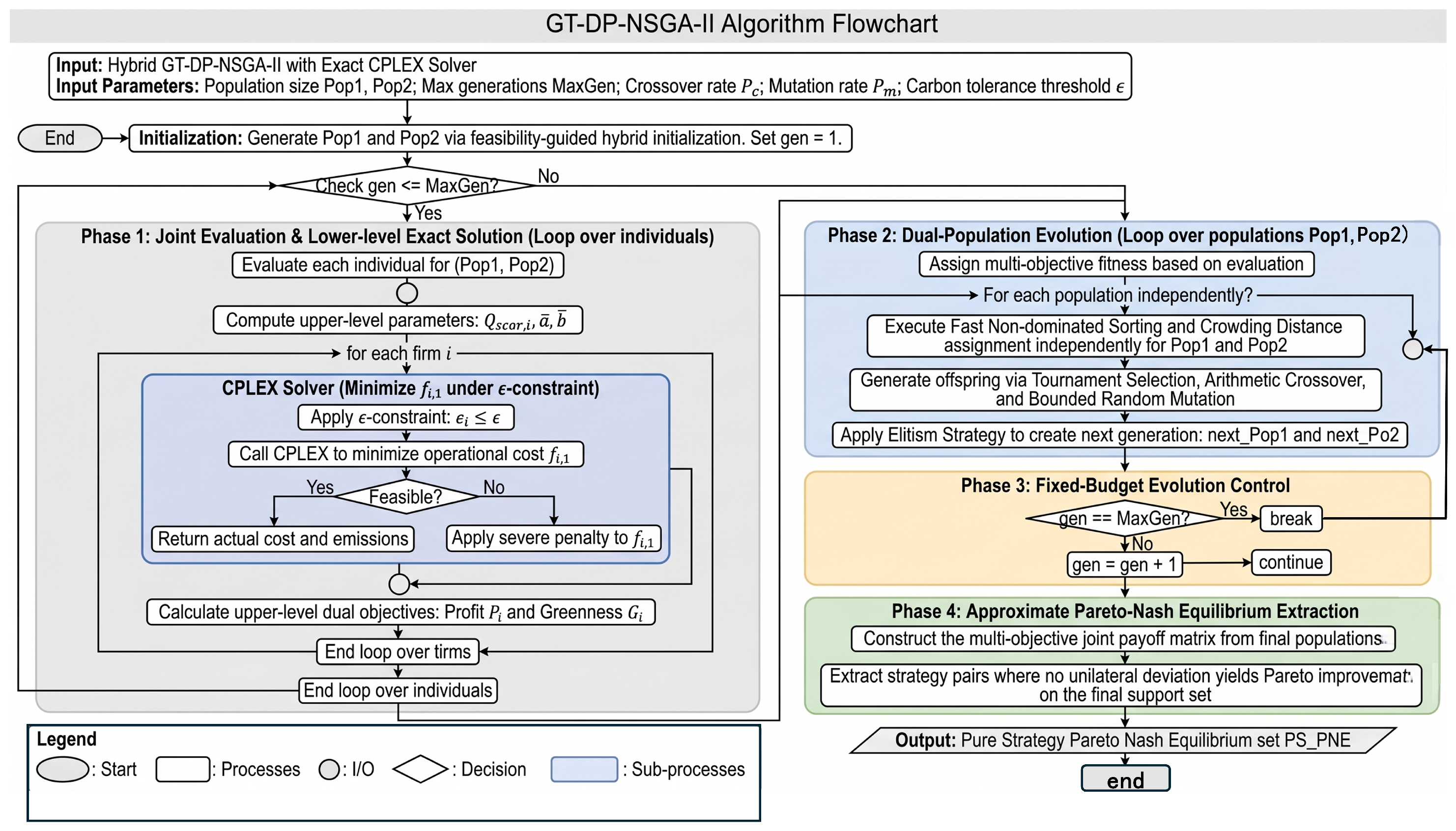
Because upper-level rivalry changes lower-level feasible regions, medium and large instances are solved by hybrid GT-DP-NSGA-II, which combines game-oriented population search with conditional lower-level optimization after $\epsilon$-constraint transformation [19,20]. For each candidate strategy pair, CPLEX solves the fixed lower-level mixed-integer subproblems, whose operating cost and emissions are fed back to the upper-level objectives. Infeasible candidates are marked as infeasible and excluded from the valid candidate pool, while the evolutionary stage updates the two populations through objective-based ranking, feasibility preference, diversity preservation, crossover, and mutation. After the final generation, the resulting finite payoff matrix is used to extract finite-candidate approximate-equilibrium pairs; local unilateral-deviation gains and safety are then computed as post-processing indicators. Thus, “conditional lower-level optimization” refers to the CPLEX-optimized subproblem for a fixed strategy pair and emission bounds, not to a closed-form or global solution of the full game [17,18].

Figure 2 summarizes the interaction between upper-level strategy generation, conditional lower-level optimization, population evolution, and finite-candidate approximate-equilibrium extraction. The hybrid GT-DP-NSGA-II procedure is summarized in Algorithm 1.

Algorithm 1. Hybrid conditional-response evolutionary procedure for the Nash-type bi-level model

Input: model parameters, upper-level bounds, lower-level data, population size $N_p$, generation limit $G_{\max }$, stabilization length $h_{\mathrm{stab}}$, crossover and mutation parameters, and lower-level emission-control parameters.

Output: finite-candidate approximate-equilibrium set.

1. Initialize two upper-level populations for the two competing supply chains and generate feasible strategic vectors.

2. Form candidate strategy pairs and decode $({\alpha }_i,{\gamma }_i,q_i,p_i,r_i)$ for each supply chain.

3. Compute induced quantities, including scarce-material allocation, subsidy allocation, demand allocation, and recovery allocation.

4. For each candidate pair, build the corresponding lower-level optimization models of the two supply chains.

5. For each candidate pair, solve the conditional lower-level cost-minimization model with the emission-control constraints generated by the $\epsilon$-constraint transformation using CPLEX.

6. If a lower-level model is infeasible, mark the corresponding upper-level candidate as infeasible and exclude it from the valid equilibrium pool; otherwise, return operating cost, emissions, and execution variables.

7. Evaluate upper-level profit and sustainability objectives using the conditional lower-level responses.

8. Apply non-dominated sorting and diversity preservation to retain high-quality candidate strategies.

9. Generate offspring through crossover and mutation, update the two populations, and set the generation counter $g\leftarrow g+1$.

10. If $g<G_{\max }$ and the generation-level stopping metrics have not stabilized for $h_{\mathrm{stab}}$ consecutive generations, go to Step 2; otherwise, stop.

11. Evaluate the final population pairs and construct the finite payoff matrix for the two supply chains.

12. Extract finite-candidate approximate-equilibrium pairs, then compute local unilateral-deviation gains, safety, and representative-selection indicators as post-processing.

13. Return the final finite-candidate approximate-equilibrium set for subsequent comparison and analysis.

Figure 2. Flowchart of the hybrid GT-DP-NSGA-II solution framework.

At the upper level, candidate strategy pairs are decoded into $({\alpha }_i,{\gamma }_i,q_i,p_i,r_i)$ and evaluated through the conditional lower-level response. During evolution, candidates are filtered by objective quality and feasibility preference; equilibrium stability is assessed only after the final candidate set has been constructed. Let the upper-level objective vector of firm i be

$$F_i(s_i,s_{-i})=\left({\pi }_i(s_i,s_{-i}),G_i(s_i,s_{-i})\right)$$

(57)

For reference, a Pareto-type generalized Nash benchmark condition for $s^{*}=(s_1^{*},s_2^{*})$ in the underlying continuous game would require $s_i^{*}\in {\mathcal{F}}_i\left(s_{-i}^{*}\right)$ and

$$\begin{array}{c}\nexists s_i\in {\mathcal{F}}_i\left(s_{-i}^{*}\right):\\ F_i(s_i,s_{-i}^{*})⪰F_i(s_i^{*},s_{-i}^{*})\end{array}$$

(58)

with at least one strict component. This continuous benchmark condition is used only as a conceptual reference. Because the strategy space is continuous and only finitely many candidates can be evaluated, the procedure uses an operational approximate-equilibrium definition based on a finite unilateral-deviation test set.

For a candidate pair $s=(s_1,s_2)$ and firm i, let ${\mathcal{D}}_i\left(s\right)$ denote the feasible deviation set generated around $s_i$. In implementation, ${\mathcal{D}}_i\left(s\right)$ is formed from bounded unilateral perturbations together with feasible nearby candidates already produced during the search. The normalization ranges are computed on the evaluation pool ${\mathcal{D}}_i\left(s\right)\cup \left\{s_i\right\}$ as

$$\begin{array}{c}\Delta {\pi }_i\left(s\right)=\underset{s_i^{\prime }\in {\mathcal{D}}_i\left(s\right)\cup \left\{s_i\right\}}{\max }\\ {\pi }_i(s_i^{\prime },s_{-i})-\underset{s_i^{\prime }\in {\mathcal{D}}_i\left(s\right)\cup \left\{s_i\right\}}{\min }\\ {\pi }_i(s_i^{\prime },s_{-i})\end{array}$$

(59)

$$\begin{array}{c}\Delta G_i\left(s\right)=\underset{s_i^{\prime }\in {\mathcal{D}}_i\left(s\right)\cup \left\{s_i\right\}}{\max }\\ G_i(s_i^{\prime },s_{-i})-\underset{s_i^{\prime }\in {\mathcal{D}}_i\left(s\right)\cup \left\{s_i\right\}}{\min }\\ G_i(s_i^{\prime },s_{-i})\end{array}$$

(60)

where a small positive constant is used if either range degenerates to zero. The normalized unilateral improvement of firm i under deviation $s_i^{\prime }$ is

$$\begin{array}{c}{r}_i^{\pi }(s_i^{\prime };s)={\displaystyle \frac{{[{\pi }_i(s_i^{\prime },s_{-i})-{\pi }_i\left(s\right)]}_{+}}{\Delta {\pi }_i\left(s\right)}},\\ r_i^G(s_i^{\prime };s)={\displaystyle \frac{{[G_i(s_i^{\prime },s_{-i})-G_i\left(s\right)]}_{+}}{\Delta G_i\left(s\right)}}\end{array}$$

(61)

where ${\left[x\right]}_{+}=\max \{x,0\}$. The corresponding unilateral-deviation pressure is defined by

$$\begin{array}{c}{\widehat{R}}_i\left(s\right)=\underset{s_i^{\prime }\in {\mathcal{D}}_i\left(s\right)}{\max }\\ \sqrt{{\displaystyle \frac{{\left(r_i^{\pi }(s_i^{\prime };s)\right)}^2+{\left(r_i^G(s_i^{\prime };s)\right)}^2}{2}}}\end{array}$$

(62)

Accordingly, the candidate is regarded as an operational approximate equilibrium if

$$\max \{{\widehat{R}}_1\left(s\right),{\widehat{R}}_2\left(s\right)\}\le \tau ,$$

(63)

where $\tau$ is fixed for the reporting rule. The reported threshold corresponds to $\underline{\mathrm{Saf}}=0.80$, or $\tau =0.20$, and is applied to the final finite candidate set as a bounded local tolerance rather than as an exhaustive continuous-space test or an internal evolutionary operator. The associated safety score is

$$\mathrm{Safety}\left(s\right)=1-\max \{{\widehat{R}}_1\left(s\right),{\widehat{R}}_2\left(s\right)\},$$

(64)

so that larger values indicate weaker unilateral-deviation incentives over the tested local deviations.

During evolution, the two populations are updated using objective ranking, feasibility preference, diversity preservation, crossover, and mutation. The procedure stops when the generation limit is reached or the generation-level ideal-point and feasibility metrics remain within tolerance for $h_{\mathrm{stab}}$ consecutive generations. Only after this stopping condition is the final finite payoff matrix used for equilibrium extraction and local deviation/safety post-processing.

Pseudo-Codeand Implementation Details

The same conditional lower-level optimization workflow is used throughout. Infeasible strategic candidates are marked infeasible and excluded from valid candidate screening rather than repaired. Finite-candidate approximate-equilibrium extraction is performed on the final finite candidate set, while safety and local unilateral-deviation measures are reported as post-processing indicators. To assess whether the fixed reporting threshold affects the conclusions, an additional post hoc robustness check is conducted on the archived medium-scale equilibrium sets by varying the safety cutoff from 0.70 to 0.90. This check does not redefine the evolutionary search process; rather, it examines whether the reported representative equilibria and key indicators are sensitive to the safety-screening cutoff.

4. Results

4.1. Case Generation and Parameter Setting

All experiments were implemented in Python 3.10 with IBM ILOG CPLEX 22.1 on a workstation with an AMD Ryzen 9 HX-series processor and 16 GB RAM. All compared algorithms used the same environment.

Three benchmark instances were constructed from public data sources and public case information, with limited and traceable adjustments to fit the present duopoly setting. The small instance is used for finite-grid calibration, the Chengdu-medium instance for the main benchmark and model comparison, and the Yangtze River Delta large instance for scalability testing. These cases are computational benchmarks adapted from public information, not direct replications of firm-level observations. Table 3 reports only the structural dimensions of the three cases.

Table 3. Benchmark case settings used in the computational experiments.

Case	Scale	Lines K	Schemes S	Ratios E	Routes T	Nodes Z	Modes M
Validation-small	Small	2	2	2	2	3	2
Chengdu-medium	Medium	8	3	3	4	20	3
YRD-large	Large	14	4	4	5	41	5

The three cases share the same modelling logic but differ in decision-space size, network density, and resource scale. The medium and large cases follow public-data-based benchmark configurations with only necessary structural adjustment, while the small case compresses the same decision structure so that exact enumeration remains feasible.

A parameter-level provenance and calibration table is provided as Supplementary Material S1. Table 4 reports the case-level provenance overview. It distinguishes public case anchors, benchmark-calibrated values, model units, transformation rules, and parameters that are active in the formal experiments. The main-text table is intentionally retained as a concise case-level overview. Supplementary Materials S2–S4 provide quality-metric audits, robustness checks, and the computational-effort audit, respectively. These Supplementary Materials are provided separately from the reproduction archive; the archived reproduction package, which contains the code, configurations, data, figures, and archived outputs used for replication, is publicly available at https://doi.org/10.6084/m9.figshare.32054619.

Table 4. Benchmark parameter provenance and calibration overview.

Case	Source Basis	Original Signal	Calibration/ Transformation	Final Benchmark Use
Validation-small	Internal validation instance	Tiny exact-enumeration benchmark	Upper-level strategy space discretized to two levels per variable; lower MILP kept in the same modelling form	Finite-grid calibration only
Chengdu-medium	Chengdu reverse-logistics case study and city-division source	More than 266,000 EVs by the end of 2021; 20 county-level divisions	Public-case scale preserved with limited structural adjustment for the homogeneous-duopoly benchmark	Main medium benchmark
YRD-large	YRD reverse-logistics case study, city-cluster overview, and NEV-output report	41-city agglomeration and large NEV manufacturing base	Scale expanded consistently with the public case and network density	Large-scale scalability test

The market-allocation function in Equation (7) uses $\beta$ as its active price-elasticity exponent. The YAML field demand_elasticity is retained for configuration compatibility and scenario metadata, but it is not an additional independent term in Equation (7) and is not treated as a separate factor in the formal sensitivity analysis. The public benchmark defines a pool of three demand scenarios, whereas the evolutionary evaluation samples one scenario per candidate through scenario_sample_count = 1; this is a computational control for the strategic comparison rather than an empirical estimate of demand uncertainty.

The benchmark instances are public-data-adapted computational cases with traceable configuration rules. Case parameters are read from the archived case YAML, while population size, generation budget, lower-level solver settings, stopping criteria, and algorithm-specific switches are read from the corresponding algorithm-specific YAML files. The pre-specified seed protocol for the formal comparison is recorded in the replication material. The archived replication package was checked against the working outputs used for the medium-scale robustness analyses, and the files "summary.json", "generation_history.csv", "pair_payoffs.csv", and "equilibria_multicriteria_unique.csv" matched the ten GT-DP-NSGA-II medium-scale seeds used in the safety-cutoff and representative-selection checks.

In the formal benchmark stage, each algorithm was run 10 times on each scale under different random seeds. The compared algorithms share the same core instance data, random-seed protocol, upper-level generation budget, and post-processing criteria, but not a common candidate-evaluation or lower-level-solver budget. Because their search architectures generate different numbers and types of candidate evaluations, the comparison reports common outcome measures together with separate workload measures. Model comparison is reported separately in Section 4.3.

The main performance indicators include runtime, the number of identified equilibria, representative total profit, representative total sustainability performance, fairness, safety, and ideal-point closeness. To keep the notation consistent with the model-comparison table, the component balance scores and their aggregate fairness score are defined by (65). In the result tables, “Rep.” means the representative equilibrium, “sust.” means sustainability performance, “Eq.” means screened equilibria, “Uniq.” means unique equilibria, and “Saf.” means the safety score defined in Equations (61)–(64).

$$\begin{array}{c}{\displaystyle F^{\pi }\left(s\right)=\frac{\min ({\pi }_1,{\pi }_2)}{\max ({\pi }_1,{\pi }_2)},F^G\left(s\right)=\frac{\min (G_1,G_2)}{\max (G_1,G_2)},}\\ {\displaystyle F\left(s\right)=\frac{1}{2}{F}^{\pi }\left(s\right)+\frac{1}{2}{F}^G\left(s\right).}\end{array}$$

(65)

The ideal-point distance is defined by (66),

$$\begin{array}{c}{d}^{\mathrm{ideal}}\left(s\right)=[{\displaystyle \frac{1}{4}}{\displaystyle \sum _{i=1}^2}(\\ {\left({\displaystyle \frac{{\pi }_i^{\mathrm{ideal}}-{\pi }_i\left(s\right)}{{\pi }_i^{\mathrm{ideal}}}}\right)}^2+{\left({\displaystyle \frac{G_i^{\mathrm{ideal}}-G_i\left(s\right)}{G_i^{\mathrm{ideal}}}}\right)}^2\\ ){]}^{1/2}\end{array}$$

(66)

where ${\pi }_i^{\mathrm{ideal}}$ and $G_i^{\mathrm{ideal}}$ are the run-specific ideal profit and sustainability references. The corresponding closeness score is defined by (67),

$$C^{\mathrm{ideal}}\left(s\right)={\displaystyle \frac{1}{1+d^{\mathrm{ideal}}\left(s\right)}},$$

(67)

so that larger values indicate better closeness.

Safety is not redefined in this section. It is the same deviation-based indicator introduced in Equations (61)–(64), evaluated on the post-analysis deviation pool; larger values indicate weaker tested unilateral-deviation incentives.

4.2. Algorithm Validation

Algorithm validation first checks whether hybrid GT-DP-NSGA-II can approach an enumerated reference equilibrium on a discretized small instance, and then compares it with two benchmark algorithms across scales.

In the validation-small instance, the five upper-level variables of each chain are discretized into two levels, yielding 32 strategies per side and 1024 strategy pairs. CPLEX post-evaluation provides a finite-grid reference equilibrium, and hybrid GT-DP-NSGA-II is tested under $G_{\max }=5$ to 37.

Table 5 shows rapid improvement from $G_{\max }=5$ to 10 and stabilization after about 10–15 generations. Ideal-point closeness increases from 0.9632 to 0.9935 at $G_{\max }=10$ and reaches 0.9964 from $G_{\max }=15$ onward, supporting the method’s credibility on the finite validation grid.

Table 5. Finite-strategy-space benchmark validation results on the discretized validation-small instance under different generation budgets.

${\mathit{G}}_{\max }$	Enum. Time	L Str.	R Str.	Pairs	Ref. Eq.	GA Time	GA Eq.	Min Dist.	Avg Dist.	Safety	Ideal Close	Profit Gap/%
5	7.414	32	32	1024	1	2.307	3	0.0698	0.0795	1.0000	0.9632	2.401
10	7.362	32	32	1024	1	3.727	2	0.0685	0.0689	1.0000	0.9935	0.283
15	7.357	32	32	1024	1	5.239	2	0.0709	0.0717	1.0000	0.9964	−0.162
20	7.515	32	32	1024	1	5.296	2	0.0709	0.0717	1.0000	0.9964	−0.162
37	7.412	32	32	1024	1	5.411	2	0.0709	0.0717	1.0000	0.9964	−0.162

The second validation task compares hybrid GT-DP-NSGA-II with Joint-NSGA-II, a unified-encoding NSGA-II benchmark [20], and NGA, a nested-search benchmark for bi-level supply chain applications [24,25]. The three methods use the same case data, random-seed protocol, upper-level generation budget, lower-level response definition, and post-processing criteria, but their search architectures do not impose a common candidate-evaluation or lower-level-solver budget. Accordingly, Table 6 reports common equilibrium-quality indicators, while runtime and solver/search counts are treated as separate workload measures. Row-wise indicators use the representative equilibrium ranked first by ideal-point closeness in each run.

Table 6. Cross-scale benchmark results of the three algorithms.

Scale	Algorithm	Time (s)	Eq. Count	Uniq. Eq.	Rep. Profit	Rep. Sust.	Fair.	Saf.	Ideal Score
Small	GT-DP-NSGA-II	316.25	6.6	2.8	7.10	2.5564	0.9381	0.9961	0.9966
Small	Joint-NSGA-II	2.83	2.5	2.5	7.63	2.5564	0.9387	0.9376	0.9442
Small	NGA	44.51	19.9	19.9	6.67	2.6451	0.9379	0.8957	0.9569
Med.	GT-DP-NSGA-II	1449.32	112.8	85.3	307.58	2.4584	0.8759	0.8389	0.9938
Med.	Joint-NSGA-II	102.73	4.0	4.0	279.17	2.2712	0.7652	0.8535	0.9580
Med.	NGA	343.88	11.0	11.0	263.83	2.1201	0.6731	0.9166	0.9068
Large	GT-DP-NSGA-II	7999.16	24.2	11.9	1031.84	4.9702	0.8060	0.9835	0.9968
Large	Joint-NSGA-II	629.06	10.3	10.3	884.37	4.7373	0.7472	0.7763	0.9295
Large	NGA	698.28	6.6	6.6	830.53	4.6288	0.7361	0.9067	0.8983

Table 6 shows a clear scale effect and should be interpreted together with Table 7. Under the common benchmark protocol, Joint-NSGA-II is fastest and attains the highest representative profit on the small instance, whereas NGA attains the highest representative sustainability performance. GT-DP-NSGA-II performs best mainly on safety and ideal-point closeness for the small instance, and on representative profit, sustainability performance, equilibrium-set size, and ideal-point closeness for the Chengdu-medium instance, although not on safety. On the YRD-large instance, it attains the highest representative profit, sustainability performance, safety, ideal-point closeness, and approximate-equilibrium set size. These quality differences indicate a quality–workload trade-off, not algorithmic superiority under an equal computational budget.

Table 7. Medium-scale computational-effort audit across the three algorithms.

Algorithm	Wall-Clock Time (s)	Upper Candidate/ Strategy-Pair Evals	Lower Response/ Function Evals	CPLEX Calls	Relative Time	Relative CPLEX Calls
GT-DP-NSGA-II	626.56 ± 75.84	18,684.30 ± 255.47	38,268.60 ± 510.95	38,268.60 ± 510.95	1.000	1.000
Joint-NSGA-II	41.16 ± 5.30	1203.70 ± 59.47	2727.40 ± 323.56	2727.40 ± 323.56	0.066	0.071
NGA	42.56 ± 10.40	1183.70 ± 37.29	770,316.00 ± 194,600.53	0	0.068	N/A

Note: Values are mean ± standard deviation over ten seeds. For GT-DP-NSGA-II and Joint-NSGA-II, lower response/function evaluations correspond to conditional lower-level CPLEX subproblem solves. For NGA, lower response/function evaluations denote heuristic lower-level plan evaluations; therefore, CPLEX calls are zero and the CPLEX-call ratio is not applicable.

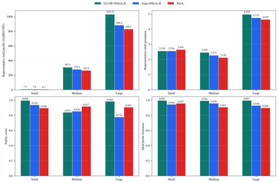
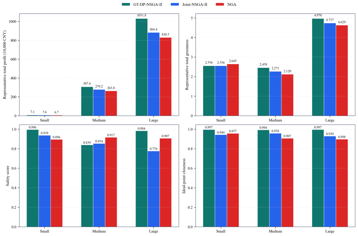
Figure 3 highlights the widening quality differences on the medium and large instances, where GT-DP-NSGA-II shows stronger representative profit and ideal-point closeness, but these gains are obtained with the higher lower-level solver burden reported in Table 7.

Figure 3. Mean algorithm-comparison results across the three benchmark scales.

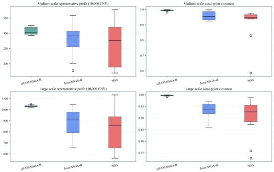
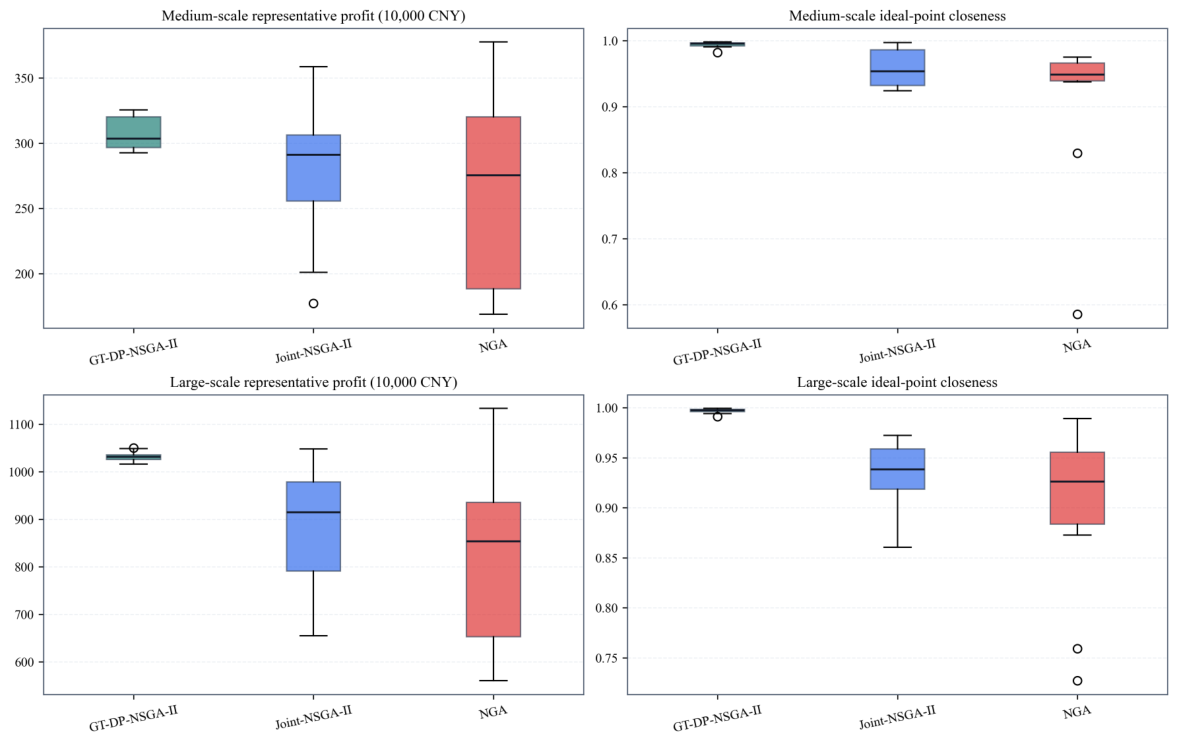
Figure 4 shows that, on both the medium and large instances, GT-DP-NSGA-II combines a relatively concentrated distribution with higher medians for representative profit and ideal-point closeness than the two baselines. This pattern supports the method’s solution-quality advantage in the present benchmark, while the workload audit clarifies the associated computational cost.

Figure 4. Run-to-run distribution of representative profit and ideal-point closeness on the medium and large instances.

A separate ten-seed medium-scale audit records the actual computational burden. GT-DP-NSGA-II required on average 626.56 s and 38,268.6 CPLEX calls per seed; Joint-NSGA-II required 41.16 s and 2727.4 calls; and NGA used a heuristic lower-level response search rather than CPLEX. Table 7 reports wall-clock time, upper-level candidate evaluations, lower-level response/function evaluations, CPLEX calls, and normalized ratios.

The audit supports a transparent workload-and-quality comparison: the methods share the benchmark protocol, but not the internal candidate-generation or lower-level response mechanism. In particular, GT-DP-NSGA-II uses substantially more CPLEX subproblem solves than Joint-NSGA-II in the medium-scale case, while NGA’s lower response/function evaluations are heuristic evaluations rather than the same computational unit. The results should therefore be read as evidence on the trade-off between solution quality and computational burden, not as an equal-budget dominance test.

Table 8 shows that tightening the safety cutoff from 0.70 to 0.90 reduces the mean retained equilibrium count from 59.8 to 23.2, as expected, and the number of non-empty seeds decreases from 10 to 8. Among the seeds that still retain at least one feasible representative equilibrium, the representative profit remains within 304.95–308.04 (${10}^4$ CNY), the representative sustainability indicator stays around 2.458, and ideal-point closeness remains above 0.990. Thus, the medium-scale conclusions are not driven by the single reporting cutoff $\mathrm{Saf}=0.80$, but the robustness statement is conditional on the retained non-empty seed set. Therefore, $\mathrm{Saf}=0.80$ is retained as a reporting threshold for the present benchmark rather than asserted to be theoretically optimal or uniquely justified.

Table 8. Post hoc robustness check under different safety cutoffs on the archived medium-scale GT-DP-NSGA-II equilibrium sets.

Safety Cutoff	Non-Empty Seeds	Mean Retained Eq.	Rep. Profit (104 CNY)	Rep. Sust.	Ideal Score	Safety Score
0.70	10	59.8	307.65	2.4585	0.9921	0.8732
0.75	9	55.9	308.04	2.4587	0.9948	0.8889
0.80	9	46.5	307.98	2.4588	0.9946	0.8920
0.85	9	38.2	307.65	2.4579	0.9940	0.9127
0.90	8	23.2	304.95	2.4586	0.9904	0.9349

A second post-processing check was performed by selecting representative equilibria using alternative criteria including safety score, fairness score, total profit, and Nash welfare. Table 9 reports the resulting mean indicators. The total sustainability-performance indicator remained in the narrow interval of 2.4569–2.4586, indicating that the main environmental-performance conclusion is stable. Representative profit, ideal-point closeness, safety, and fairness nevertheless vary with the selection criterion, so local economic, stability, and distributive interpretations based on a single representative solution remain selection-rule-dependent.

Table 9. Robustness of representative-equilibrium selection under alternative criteria.

Selection Criterion	Rep. Profit (104 CNY)	Rep. Sust.	Ideal Score	Safety Score	Fairness Score
Ideal closeness	307.58	2.4584	0.9938	0.8389	0.8759
Safety score	303.19	2.4569	0.9739	0.9302	0.8628
Fairness score	301.71	2.4570	0.9679	0.7951	0.9061
Total profit	313.57	2.4586	0.9758	0.7548	0.8658
Nash welfare	313.30	2.4575	0.9728	0.7705	0.8719

Taken together, the validation results show that hybrid GT-DP-NSGA-II is computationally credible for the present problem and that its comparative strength lies in representative-solution quality and finite-candidate approximate-equilibrium-set richness rather than speed. At the same time, the additional audit makes clear that this quality improvement is obtained with a higher computational workload, so practical use should consider the trade-off between equilibrium-set richness and lower-level solver effort.

4.3. Model Comparison

To minimize the influence of algorithmic heterogeneity, this subsection evaluates the Nash-type bi-level model ($M_1$), the Stackelberg bi-level model ($M_2$), and the centralized-cooperative model ($M_3$) on the Chengdu-medium-scale instance under the same conditional lower-level post-evaluation procedure. The focus is not on search efficiency, but on structural differences in system efficiency, allocation balance, competitive stability, and implementation feasibility.

The first group of indicators measures system efficiency and distributional balance. In Table 10, ${\mathsf{\Pi }}^{\mathrm{sys}}$ and $G^{\mathrm{sys}}$ denote system total profit and system total sustainability performance; $F^{\pi }$ and $F^G$ denote the corresponding profit- and sustainability-balance indicators; and $C^{\mathrm{op}}$ and $E^{\mathrm{tot}}$ denote the total operating cost and total carbon emissions obtained from the same conditional lower-level post-evaluation procedure. To keep each row internally consistent, $F^{\pi }$ and $F^G$ are recomputed from the reported mean values of $({\pi }_1,{\pi }_2)$ and $(G_1,G_2)$ rather than averaged separately across runs.

Table 10. Core comparison of the three model structures on the Chengdu-medium-scale instance.

Model	Upper-Level Structure	${\mathsf{\Pi }}^{\mathbf{sys}}$	${\mathit{G}}^{\mathbf{sys}}$	${\mathit{\pi }}_1$	${\mathit{\pi }}_2$	${\mathit{G}}_1$	${\mathit{G}}_2$	${\mathit{F}}^{\mathit{\pi }}$	${\mathit{F}}^{\mathit{G}}$	${\mathit{C}}^{\mathbf{op}}$	${\mathit{E}}^{\mathbf{tot}}$
$M_1$	Nash-type bi-level	307.58	2.4584	166.02	141.56	1.2732	1.1852	0.8526	0.9309	210.79	41.85
$M_2$	Stackelberg bi-level	251.56	2.3171	121.83	129.73	1.1381	1.1790	0.9391	0.9653	190.63	38.30
$M_3$	Centralized-cooperative	332.05	2.2809	209.69	122.36	1.2302	1.0508	0.5835	0.8542	132.98	28.72

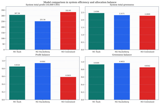
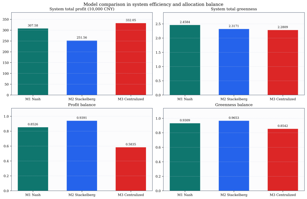
Table 10 shows distinct structural effects. $M_3$ gives the coordinated profit and cost benchmark, $M_1$ yields the highest system sustainability performance, and $M_2$ produces the strongest allocation balance.

Figure 5 visualizes these differences in system efficiency and allocation balance.

Figure 5. Comparison of system efficiency and allocation-balance indicators across the three models.

The second group of indicators examines competitive stability, leader-role sensitivity, and implementation feasibility. For this purpose, a local unilateral-deviation test is conducted around each representative solution. Let ${\mathcal{N}}_i$ denote the neighbourhood generated by small perturbations of the upper-level decision vector of supply chain i while holding the rival strategy fixed. The unilateral profit-deviation gain and unilateral sustainability-deviation gain are defined as

$${\Delta }_i^{\pi ,\mathrm{loc}}=\underset{s_i^{\prime }\in {\mathcal{N}}_i}{\max }{\left[{\pi }_i(s_i^{\prime },s_{-i})-{\pi }_i(s_i,s_{-i})\right]}_{+}$$

(68)

$${\Delta }_i^{G,\mathrm{loc}}=\underset{s_i^{\prime }\in {\mathcal{N}}_i}{\max }{\left[G_i(s_i^{\prime },s_{-i})-G_i(s_i,s_{-i})\right]}_{+}$$

(69)

where smaller values indicate that the reported solution is less vulnerable to being broken by unilateral local adjustment. These raw local gains are distinct from the normalized deviation components used in the safety score in Equations (61)–(64). To record whether a local deviation can improve both objectives simultaneously, the number of Pareto-improving unilateral deviations is defined as

$$\begin{array}{c}{N}_i^{PD}=\mathrm{card}\{s_i^{\prime }\in {\mathcal{N}}_i:{\pi }_i^{\prime }\ge {\pi }_i,G_i^{\prime }\ge G_i,\\ ({\pi }_i^{\prime },G_i^{\prime })\ne ({\pi }_i,G_i)\}\end{array}$$

(70)

For the Stackelberg model, leader-role sensitivity is evaluated by switching the designated leader between the two supply chains. Let $Z^{L1}$ and $Z^{L2}$ denote the same performance indicator under the two alternative role assignments. Then the role-sensitivity indicator is defined as

$$RS\left(Z\right)={\displaystyle \frac{|Z^{L1}-Z^{L2}|}{\max \left(\right|Z^{L1}|,|Z^{L2}\left|\right)+{10}^{-6}}}$$

(71)

Larger values of $RS\left(Z\right)$ indicate that the model result depends more strongly on the exogenously imposed leader identity. For the centralized-cooperative model, implementation feasibility is examined relative to the Nash benchmark. The participation gap of supply chain i and the minimum compensation requirement are defined as

$$P{G}_i=\max \left\{0,{\pi }_i^{Nash}-{\pi }_i^{Cent}\right\}$$

(72)

$$T{C}_{\min }={\displaystyle \sum _{i=1}^2}P{G}_i$$

(73)

If $P{G}_i$ or $T{C}_{\min }$ is large, the centralized solution may remain efficient at the system level but difficult to implement voluntarily under competition. In the numerical test, the local unilateral-deviation neighbourhood is constructed under both $\pm 5\%$ and $\pm 10\%$ perturbation radii around the representative upper-level strategy of each supply chain, whereas the role-sensitivity and participation-gap indicators are reported only once because they do not depend on the perturbation radius.

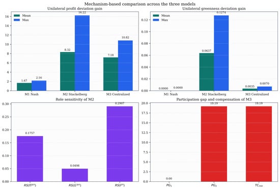
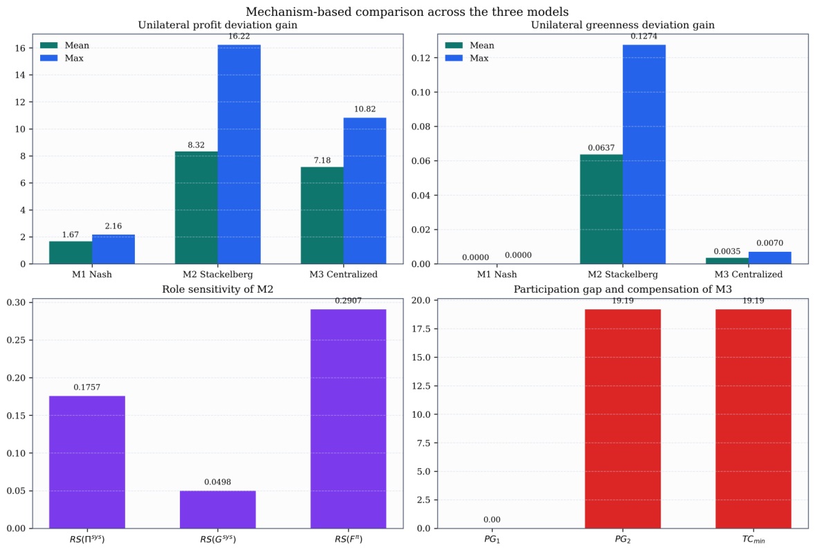
Table 11 shows that $M_1$ has the smallest unilateral-deviation gains, $M_2$ remains sensitive to leader assignment, and $M_3$ retains a positive participation gap under both perturbation radii. The three structures are therefore better interpreted by environmental suitability than by universal ranking.

Table 11. Stability, role-sensitivity, and implementation-feasibility tests for the three models on the Chengdu-medium-scale instance.

Model	Radius	Mean ${\mathbf{\Delta }}_{\mathbf{loc}}^{\mathit{\pi }}$	Max ${\mathbf{\Delta }}_{\mathbf{loc}}^{\mathit{\pi }}$	Mean ${\mathbf{\Delta }}_{\mathbf{loc}}^{\mathit{G}}$	Max ${\mathbf{\Delta }}_{\mathbf{loc}}^{\mathit{G}}$	Total ${\mathit{N}}^{\mathbf{PD}}$	$\mathit{RS}$ $\left({\mathsf{\Pi }}^{\mathbf{sys}}\right)$	$\mathit{RS}$ $\left({\mathit{G}}^{\mathbf{sys}}\right)$	$\mathit{RS}$ $\left({\mathit{F}}^{\mathit{\pi }}\right)$	${\mathit{PG}}_1$	${\mathit{PG}}_2$	${\mathit{TC}}_{\min }$
$M_1$	$\pm 5\%$	1.67	2.16	0.0000	0.0000	74	–	–	–	–	–	–
	$\pm 10\%$	1.74	2.54	0.0000	0.0000	63	–	–	–	–	–	–
$M_2$	$\pm 5\%$	8.32	16.22	0.0637	0.1274	41	0.1757	0.0498	0.2907	–	–	–
	$\pm 10\%$	10.63	20.51	0.0637	0.1274	40	–	–	–	–	–	–
$M_3$	$\pm 5\%$	7.18	10.82	0.0035	0.0070	73	–	–	–	0.00	19.19	19.19
	$\pm 10\%$	12.70	18.92	0.0070	0.0140	72	–	–	–	–	–	–

Figure 6 confirms this pattern: centralized coordination provides an efficiency benchmark, Stackelberg captures hierarchy, and the Nash-type bi-level model is most consistent with the present homogeneous-duopoly setting because this benchmark assumes comparable firms and simultaneous competition. This statement is limited to the stylized homogeneous parallel-competition benchmark used in this study and should not be interpreted as empirical verification or industry-level identification of a Nash-type structure.

Figure 6. Mechanism-based comparison of competitive stability, role sensitivity, and implementation feasibility.

4.4. Sensitivity Analysis

We conduct an eight-factor single-factor sensitivity analysis on the Chengdu-medium-scale instance, using five equally spaced levels and seeds 5, 37, and 70. The three seeds were selected from the formal ten-seed protocol to cover representative low-, middle-, and high-index search trajectories while keeping the additional computational burden manageable. Because this analysis uses three replications rather than the ten seeds used in the main algorithm comparison, the results are interpreted as directional and benchmark-specific evidence. For weak or non-monotonic responses, stochastic search variation cannot be fully separated from genuine parameter sensitivity. Because sustainability performance is already embedded in the upper-level formulation, the analysis focuses on changes in representative profit, realized emissions, and equilibrium structure rather than derivative-style local sensitivity. Table 12 reports the tested ranges, affected indicators, and dominant observed patterns.

Table 12. Evidence summary of the eight sensitivity factors.

Parameter	Range	Affected Indicators	Main Phenomenon
Expected market demand	17,024–25,536	Total profit; average unit total emission; market quantities	Total profit rises sharply, while average unit total emission remains nearly flat.
Scarce-material supply	126–294	Total profit; native and recycled-material use; profit balance	Profit falls as supply is relaxed, and the material mix shifts between native and recycled inputs.
Government subsidy	0–600,000 CNY	Total profit; profit balance; average unit total emission	Profit improves with subsidy, but the emission response remains limited.
Carbon-emission standard	14.0–20.0	Total sustainability performance; average unit total emission; total profit	Sustainability performance changes clearly, whereas actual average unit total emission stays within a narrow band.
Consumer green preference	0.6–1.4	Unique equilibria; profit balance; total profit	The number of equilibria increases markedly, while the environmental response remains weak.
Low-carbon transport cost coefficient	0.50–1.50	Total profit; right unit transport emission	The response is weak and mainly structural rather than monotonic.
Recovery yield factor	0.80–1.20	Total profit; system recycled-material share	The material-share response is limited under the current case setting.
Demand elasticity ($\beta$)	0.6–1.4	Total profit; market-share gap; unique equilibria	Profit and market allocation vary non-monotonically, while the environmental response remains limited.

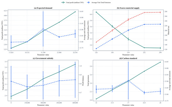
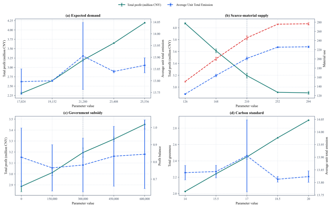
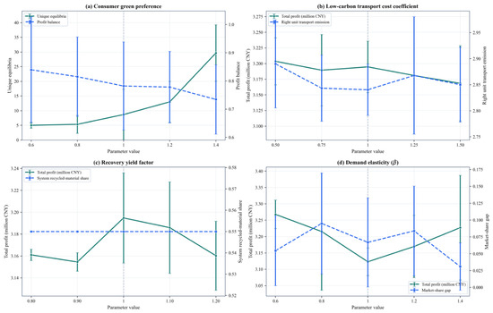
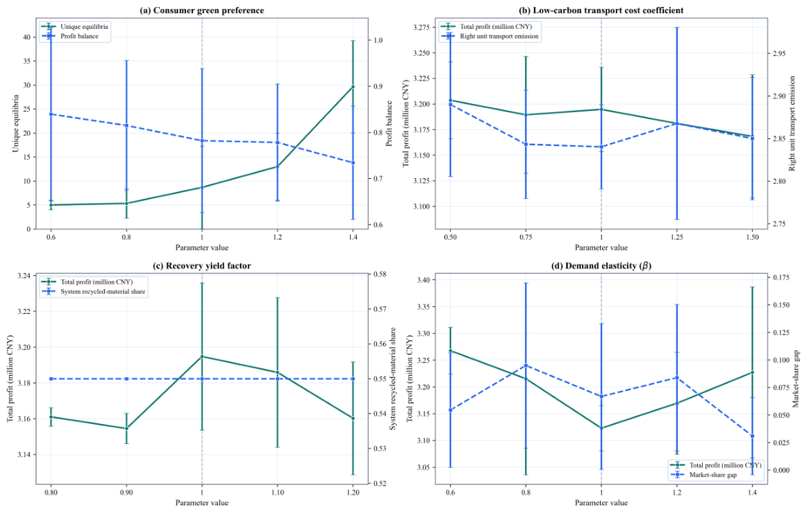
Expected demand has the clearest directional effect: higher demand raises representative total profit, while average unit total emission changes only mildly. Scarce-material supply mainly changes the native–recycled-material mix and the associated profit balance. The counter-intuitive profit decrease observed when scarce-material supply is relaxed is not interpreted as a general economic law. In this benchmark, scarce-material allocation is endogenous to bidding behaviour, recycled-material substitution, and representative-equilibrium selection; relaxing one shared resource can therefore move the reported solution to a different finite-candidate equilibrium with a different cost and allocation structure. Government subsidy raises profit but has limited impact on average unit total emission; the carbon-emission standard changes the sustainability-performance score more visibly than realized emission intensity; and consumer green preference mainly affects equilibrium multiplicity and profit balance. Demand elasticity changes total profit and the market-share gap without a comparable change in realized emissions. Under the endogenous-sustainability setting, these policy and preference parameters therefore act primarily as profit- and structure-shifters.

The low-carbon transport cost coefficient and recovery yield factor show weak marginal effects, expressed mainly through transport or material composition. Across the eight factors, demand scale and material scarcity are the clearest directional drivers, whereas subsidy, carbon standard, consumer sustainability preference, demand elasticity, and isolated technical parameters have limited direct influence on realized emissions. Under the modeled conditions, materially lower emissions are more likely to require a broader feasible set of low-carbon production, recycling, and transport options. Figure 7 and Figure 8 show the three-seed means; error bars denote one standard deviation and dashed vertical lines mark the baseline. The figure-level evidence should therefore be read as directional rather than as a full ten-seed stochastic robustness test.

Figure 7. Sensitivity responses to market, resource, subsidy, and emission-standard parameters under the three-seed directional check (panels (a)–(d)).

Figure 8. Sensitivity responses to consumer preference, operational parameters, and demand elasticity under the three-seed directional check (panels (a)–(d)).

5. Discussion

For the stylized homogeneous-duopoly setting, the Nash-type bi-level formulation is more consistent than a forced leader–follower or centralized-cooperative structure because no upper-level leader is imposed and operational responses remain explicit. This conclusion follows from the homogeneous and simultaneous-competition assumptions embedded in the benchmark and should not be read as empirical identification of the actual power-battery industry’s competitive structure. Stackelberg models remain appropriate when power asymmetry or first-mover commitment exists [5,6,8]. The sensitivity analysis further identifies demand and resource scarcity as the clearest directional drivers, while subsidy, carbon standard, consumer sustainability preference, demand elasticity, and isolated technical parameters mainly reshape profit allocation, equilibrium multiplicity, or feasible operating combinations.

The managerial implications are conditional on the source of disturbance. Under the modeled conditions, when demand expansion or scarce-material tightness is the main pressure, it may be appropriate to prioritize procurement bidding and the allocation of native and recycled materials, because these factors produce the clearest changes in profit and material structure. When the policy objective is to reduce realized emissions rather than compensate firms, the benchmark results suggest that subsidies and consumer-preference incentives may need to be paired with a wider set of low-carbon production, recycling, and transport options; isolated financial incentives mainly shift profit and market allocation under the present endogenous-sustainability setting. Central coordination is implementable only when the participation gap of the disadvantaged chain can be compensated, whereas a Nash-type structure is more appropriate for structurally comparable competitors without a designated leader in the stylized benchmark.

6. Conclusions

This study develops a Nash-type bi-level framework for two competing cleaner closed-loop power-battery supply chains, linking simultaneous strategic decisions with lower-level production, recycling, transportation, inventory, and emission responses. The results support three bounded conclusions: the Nash-type structure is consistent with the assumed homogeneous parallel rivalry; operational feasibility is best evaluated jointly with strategic decisions; and demand and material scarcity have the clearest directional effects, whereas policy, preference, and isolated technical parameters mainly reshape profit allocation, equilibrium multiplicity, and feasible operating combinations. The robustness checks also show that sustainability-performance conclusions are relatively stable across representative-selection rules, while some economic, stability, and distributive interpretations based on a single representative solution remain selection-rule-dependent.

The study contributes by integrating shared-constraint Nash-type competition with explicit lower-level operational response evaluation. The work remains limited to a static complete-information setting with two stylized homogeneous supply chains; the computational cases are adapted from public information and are not direct firm-level empirical observations or industry-wide empirical samples. In addition, the sensitivity analysis uses three representative seeds and therefore provides directional benchmark evidence rather than a full stochastic robustness proof. Future research may consider dynamic or stochastic games, incomplete information, heterogeneous firms, richer policy instruments, and broader replication of sensitivity experiments.

References

- Gu, X.; Ieromonachou, P.; Zhou, L.; Tseng, M.L. Developing pricing strategy to optimise total profits in an electric vehicle battery closed loop supply chain. J. Clean. Prod. 2018, 203, 376–385. [Google Scholar] [CrossRef] [Scilit]
- Scheller, C.; Schmidt, K.; Spengler, T.S. Effects of network structures on the production planning in closed-loop supply chains: A case study based analysis for lithium-ion batteries in Europe. Int. J. Prod. Econ. 2023, 264, 108892. [Google Scholar] [CrossRef] [Scilit]
- Tajik, M.; Yousefi, S.; Tosarkani, B.M.; Makui, A. Digitalization-driven circular economy in battery closed-loop supply chain network design. J. Clean. Prod. 2025, 500, 145054. [Google Scholar] [CrossRef] [Scilit]
- Yoo, S.H.; Cheong, T. Inventory model for sustainable operations of a closed-loop supply chain: Role of a third-party refurbisher. J. Clean. Prod. 2021, 312, 127810. [Google Scholar] [CrossRef] [Scilit]
- Wang, N.; He, Q.; Jiang, B. Hybrid closed-loop supply chains with competition in recycling and product markets. Int. J. Prod. Econ. 2019, 217, 246–258. [Google Scholar] [CrossRef] [Scilit]
- Xiao, M.; Xu, C.; Xie, F. Research on the impact of information sharing and government subsidy on competitive power battery recycling. J. Clean. Prod. 2024, 452, 142989. [Google Scholar] [CrossRef] [Scilit]
- Liu, K. How government intervention and supply chain competition and cooperation affect power battery recycling from a game theory perspective? Int. J. Low.-Carbon Technol. 2025, 20, ctaf059. [Google Scholar] [CrossRef] [Scilit]
- Hu, K.; Hou, Q. Decision-making of power battery closed-loop supply chain considering corporate social responsibility and echelon utilization. Mod. Supply Chain Res. Appl. 2025, 7, 346–371. [Google Scholar] [CrossRef] [Scilit]
- Facchinei, F.; Kanzow, C. Generalized Nash equilibrium problems. 4OR 2007, 5, 173–210. [Google Scholar] [CrossRef] [Scilit]
- Facchinei, F.; Fischer, A.; Piccialli, V. On generalized Nash games and variational inequalities. Oper. Res. Lett. 2007, 35, 159–164. [Google Scholar] [CrossRef] [Scilit]
- Shekarian, E. A review of factors affecting closed-loop supply chain models. J. Clean. Prod. 2020, 246, 119823. [Google Scholar] [CrossRef] [Scilit]
- Alegoz, M.; Kaya, O.; Bayindir, Z.P. Closing the loop in supply chains: Economic and environmental effects. Comput. Ind. Eng. 2020, 142, 106366. [Google Scholar] [CrossRef] [Scilit]
- Pakseresht, M.; Shirazi, B.; Mahdavi, I.; Mahdavi-Amiri, N. Toward sustainable optimization with Stackelberg game between green product family and downstream supply chain. Sustain. Prod. Consum. 2020, 23, 198–211. [Google Scholar] [CrossRef] [Scilit]
- Saxena, N.; Sarkar, B.; Wee, H.M.; Reong, S. A reverse logistics model with eco-design under the Stackelberg-Nash equilibrium and centralized framework. J. Clean. Prod. 2023, 386, 135789. [Google Scholar] [CrossRef] [Scilit]
- Abbasi, N.; Lotfi, M.M.; Shishebori, D.; Forghani, A. A Stackelberg-Nash game framework for overcoming remanufacturing barriers in a duopoly. J. Dyn. Games 2025, 17, 156–186. [Google Scholar] [CrossRef] [Scilit]
- Calvete, H.I.; Galé, C.; Iranzo, J.A. Planning of a decentralized distribution network using bilevel optimization. Omega 2014, 49, 30–41. [Google Scholar] [CrossRef] [Scilit]
- Setak, M.; Feizizadeh, F.; Tikani, H.; Shaker Ardakani, E. A bi-level stochastic optimization model for reliable supply chain in competitive environments: Hybridizing exact method and genetic algorithm. Appl. Math. Model. 2019, 75, 566–590. [Google Scholar] [CrossRef] [Scilit]
- Sinha, A.; Malo, P.; Deb, K. Evolutionary algorithm for bilevel optimization using approximations of the lower level optimal solution mapping. Eur. J. Oper. Res. 2017, 257, 395–411. [Google Scholar] [CrossRef] [Scilit]
- Mavrotas, G. Effective implementation of the ε-constraint method in multi-objective mathematical programming problems. Appl. Math. Comput. 2009, 213, 455–465. [Google Scholar] [CrossRef] [Scilit]
- Deb, K.; Pratap, A.; Agarwal, S.; Meyarivan, T. A fast and elitist multiobjective genetic algorithm: NSGA-II. IEEE Trans. Evol. Comput. 2002, 6, 182–197. [Google Scholar] [CrossRef] [Scilit]
- Feng, Z.; Xiao, T.; Robb, D.J. Environmentally responsible closed-loop supply chain models with outsourcing and authorization options. J. Clean. Prod. 2021, 297, 123791. [Google Scholar] [CrossRef] [Scilit]
- Desyanti, R.; Suparno; Arvitrida, N.I. Pricing decisions in closed-loop supply chains: A game theory perspective through scoping review and bibliometric analysis. Appl. Oper. Anal. 2025, 2, 1–22. [Google Scholar] [CrossRef] [Scilit]
- Konak, A.; Kulturel-Konak, S.; Snyder, L.V. A Game-Theoretic Genetic Algorithm for the reliable server assignment problem under attacks. Comput. Ind. Eng. 2015, 85, 73–85. [Google Scholar] [CrossRef] [Scilit]
- Zhang, Y.; Wang, J.; Lim, M.K.; Tseng, M.L. Joint production planning, pricing and retailer selection with emission control based on Stackelberg game and nested genetic algorithm. Expert Syst. Appl. 2020, 157, 113733. [Google Scholar] [CrossRef] [Scilit]
- Jiao, J.; Yang, D.; Zhang, Y. A Stackelberg game theoretic model for optimizing product family architecting with supply chain consideration. Int. J. Prod. Econ. 2016, 172, 1–18. [Google Scholar] [CrossRef] [Scilit]
Disclaimer/Publisher’s Note: The statements, opinions and data contained in all publications are solely those of the individual author(s) and contributor(s) and not of MDPI and/or the editor(s). MDPI and/or the editor(s) disclaim responsibility for any injury to people or property resulting from any ideas, methods, instructions or products referred to in the content. |
© 2026 by the authors. Licensee MDPI, Basel, Switzerland. This article is an open access article distributed under the terms and conditions of the Creative Commons Attribution (CC BY) license.