


Abstract
Background: The rapid evolution of omnichannel retailing has reshaped retail supply chains (SCs) by coupling replenishment, fulfillment, and service decisions across multiple demand channels under inventory, lead-time, and capacity constraints. These interdependencies create coordination challenges, particularly when demand shocks interact with limited operational capacity. Methods: To address these challenges, this study develops a centralized Hierarchical Reinforcement Learning (HRL) control framework that makes decision timing explicit: replenishment and allocation are optimized weekly, while fulfillment and lateral inventory rebalancing are controlled daily. Policies are learned using Proximal Policy Optimization (PPO) in an actor–critic architecture, with bounded stochastic policies for constrained action spaces. To mitigate the curse of dimensionality in HRL, we introduce a capacity-aware state–action encoding mechanism that compresses the control interface into structured summary signals. Demand shocks are modeled using two specifications: a mixed profile, where half the products follow a uniform demand process and the rest a Merton-type jump-diffusion process, and a fully shock-driven profile. Results: The framework is evaluated against forecast-driven base-stock and greedy fulfillment heuristics, and a perfect-information oracle, with pairwise differences examined through Wilcoxon signed-rank tests. Conclusions: Overall, the proposed framework improves learning efficiency and scalability, outperforming heuristic baselines while remaining below the oracle bound.
1. Introduction
The modern retail supply chain (SC) has undergone a fundamental shift, especially due to the rise of electronic retailing and digitally enabled fulfillment networks. E-tailers (electronic retailers) serve a key role in the online shopping landscape today by providing digital platforms through which consumers can conveniently search, compare, and purchase products online. In particular, an e-tailer is an online retail platform that sells products directly to consumers while potentially hosting third-party sellers on the same platform, thus combining retailing and marketplace functions [1]. In this landscape, traditional brick-and-mortar retailers and pure e-tailers increasingly function within interconnected distribution ecosystems that require tight coordination of inventory, logistics, and customer service decisions across spatially dispersed nodes. Early empirical evidence indicates that retailers have been progressively restructuring their physical distribution processes to support this new environment, for example, by integrating store and distribution center inventories and leveraging retail stores as forward fulfillment nodes to enhance last-mile responsiveness [2]. These developments have significantly increased operational interdependencies within retail SCs and have created new challenges for inventory positioning, demand fulfillment, and network coordination. At the same time, recent developments in logistics and operations management highlight a broader shift toward data-driven and AI-enabled support tools, further including context-aware demand forecasting and data-driven SC mapping approaches. Although these methods primarily focus on improving the accuracy and visibility of the prediction network, they further underline the increasing complexity and intensity of information in modern retail systems [3,4].
The operational importance of this problem is further underscored by recent market evidence. On a worldwide scale, the share of retail sales represented by e-commerce was estimated to have increased from 10.4% in 2017 to 14.1% in 2019 and was projected to reach 21.0% in 2025, indicating that digital channels now account for a substantial and growing part of retail activity [5]. At the same time, official U.S. statistics show that retail e-commerce sales reached $1.2337trillion in 2025, increasing by 5.4% over 2024 and accounting for 16.4% of total retail sales [6]. This growth does not imply the disappearance of physical retail; rather, consumers increasingly combine digital and in-store purchasing modes, further strengthening the need for tightly coordinated omnichannel fulfillment systems [7].
Building on this evolution, omnichannel retailing has emerged as a dominant paradigm in which firms simultaneously manage physical and digital channels within a unified customer experience and operational framework [8]. The rapid growth of omnichannel systems during the last decade has introduced substantial complexity due to cross-channel demand substitution, multi-location inventory coupling, and capacity-constrained fulfillment decisions. Recent research shows that commonly adopted strategies such as ship-from-store and buy-online-pick-up-in-store (BOPIS) can create significant value, but their effectiveness depends critically on demand structure, cost parameters, and inventory allocation capabilities [9]. At the same time, studies examining BOPIS adoption, channel coordination, and demand interactions highlight that omnichannel performance is highly sensitive to substitution effects, encroachment dynamics, and nonlinear demand behavior [10,11]. These findings underscore the need for more sophisticated operational decision-making frameworks capable of managing the tightly coupled and stochastic nature of omnichannel environments.
Another critical aspect of omnichannel SC systems is the temporal hierarchy of decision-making. In SC and production planning research, this idea is closely related to the notion of temporal integration, namely the coordination of decisions across different timescales and decision-making levels, such as strategic, tactical, and operational ones [12]. A similar temporal structuring also appears in other supply-chain functions, including forecasting, where demand estimates support inventory- and production-oriented planning, service-level management, and broader decision-support processes across the different hierarchies commonly identified in SCs [13]. These particularities are especially prevalent in multi-echelon systems that are not only spatially or organizationally distributed, but also temporally structured. Higher-level decisions are usually more aggregate and slower-moving, whereas lower-level decisions are more detailed, more reactive, and more closely tied to real-time operating conditions. Recent work on multi-layer planning similarly emphasizes that monthly, weekly, and daily decision layers serve different planning purposes and must remain aligned in order to support effective execution under uncertainty [14]. This distinction is particularly important in omnichannel SCs, where upstream decisions such as replenishment planning, inventory positioning, and allocation are subject to lead times and capacity restrictions, while downstream decisions such as fulfillment, order routing, and local transshipment must respond more quickly to realized demand.
Despite the growing operational importance of omnichannel systems, the corresponding analytical and data-driven decision literature remains largely fragmented. For example, a growing body of work has examined coordination and inventory decisions through game-theoretic approaches, bilevel optimization, simulation–optimization, and nonlinear programming approaches [15,16,17,18,19,20,21]. Although these studies provide valuable structural insights, they mainly rely on static analytical formulations or offline optimization procedures, which are inadequate for capturing the multi-period, stochastic, and dynamically evolving nature of modern omnichannel fulfillment systems. At the same time, recent studies have begun to explore reinforcement learning (RL) and other adaptive control schemes in omnichannel settings. However, these contributions remain largely inadequate in their ability to capture realistic network complexity, including multi-echelon inventory interactions, lateral rebalancing, capacity-coupled fulfillment dynamics, and the explicit representation of temporally differentiated decision layers [22,23,24,25]. Note also that most existing approaches focus on simplified network structures or single-level decision processes, limiting their applicability to integrated omnichannel systems. This gap is particularly critical in capacity-constrained omnichannel environments, where decisions interact across multiple time scales and high-dimensional state spaces, thus making integrated control increasingly challenging.
Motivated by these limitations, the present study develops a Hierarchical Reinforcement Learning (HRL) framework to support coordinated replenishment and fulfillment decisions in capacity-constrained omnichannel retail networks. In particular, the main contribution of the study is the development of an HRL decision framework that explicitly captures the multi-timescale nature of omnichannel operations by decomposing weekly replenishment planning and daily fulfillment control into coordinated managerial layers. Unlike existing RL-based approaches that typically rely on simplified network representations or single-level decision processes, the proposed framework enables integrated control across multiple echelons, decision layers, and operational constraints. Building upon this central contribution, the paper also introduces an integrated omnichannel modeling environment that considers physical stores, a centralized fulfillment center (FC), and multiple demand channels under explicit inventory and processing capacity constraints, while also incorporating lateral inter-store transshipment as a dynamic inventory rebalancing mechanism. The study evaluates the proposed framework under shock-prone demand conditions through a Merton-type process and benchmarks its performance against flat PPO, business-relevant heuristics, and a perfect-information oracle. Arguably, these elements demonstrate how hierarchical control enables more effective coordination in complex, capacity-constrained omnichannel systems, leading to improved service performance and profitability and thereby extending the applicability of RL-based methods in data-driven retail operations. To summarize, the main contributions of this study are as follows:
- We develop an HRL framework that captures multi-timescale decision-making by coordinating replenishment and fulfillment.
- We propose an integrated omnichannel model with stores, a fulfillment center, multiple demand channels, and explicit capacity constraints and we further incorporate lateral transshipment as a dynamic inventory rebalancing mechanism.
- We extend RL-based approaches to multi-echelon, capacity-coupled, and hierarchical control settings.
- We evaluate performance under shock-prone demand and benchmark against PPO, heuristics, and a perfect-information oracle.
- We provide managerial insights on coordinated control in capacity-constrained omnichannel systems.
The remainder of the paper is organized as follows. Section 2 provides background information and a literature review, first discussing the distinction between RL and HRL through the lens of temporal abstraction and multi-timescale decision-making, and then reviewing the relevant RL-centric literature on omnichannel SCs. Section 3 formulates the studied omnichannel problem, presents the network structure, decision variables, objective function, sources of uncertainty, and the underlying constrained operations model. Section 4 introduces the proposed HRL framework, develops the corresponding MDP representation, and details the state and action spaces, the architectural design, and the PPO-based implementation. Section 5 presents the adopted benchmarking protocol, reports the experimental evaluation, and analyzes the numerical results obtained across different capacity configurations, demand rates, and store scales, while also examining how node-specific capacities affect network resilience. Section 6 discusses the main findings, managerial implications, study limitations, and future research directions, and Section 7 concludes the paper.
2. Background Information and Literature Review
Our work builds on the premise that Hierarchical Reinforcement Learning (HRL) may be a well-suited solution approach for SCs, where decision hierarchies naturally arise from the underlying business model and organizational structure. In omnichannel SCs, such hierarchical policies also emerge operationally, as product flows and fulfillment responsibilities are coordinated across multiple echelons and time scales. For this reason, explicitly accounting for the temporal hierarchy of decision-making provides a stronger justification for HRL in omnichannel SCs, as HRL can align the control architecture with the multi-layer temporal logic of the system by assigning slower, higher-level policies to aggregate planning decisions and faster, lower-level policies to operational execution. Building on this perspective, this section first highlights the key differences between RL and HRL agentic schemes through the lens of how decision timing is structured across levels. It then reviews the existing RL-centric literature relevant to omnichannel SCs to illustrate ways forward beyond the current state of the art.
2.1. HRL vs. RL: Temporal Hierarchy of Decision-Making in Supply Chains
RL represents one of the most-studied paradigms in the recent ML literature, designed to capture how an intelligent agent acquires decision-making competence through repeated interaction with an environment and feedback on the consequences of its actions. Most RL formulations are grounded in the Markov Decision Process (MDP) framework, which models sequential decision-making under uncertainty through the tuple , where denotes the state space, the action space, the transition dynamics, the reward function, and a discount factor that determines the relative importance of future outcomes. At each time step t, the agent observes , selects according to a policy , receives a scalar reward , and transitions to . The learning objective is to identify a policy that maximizes the expected long-term return, typically defined as the discounted cumulative reward , thereby balancing short-term gains and longer-term performance [26]. This functionality has been found to be particularly relevant to SC management, where many problems preserve a sequential and progressive nature; accordingly. In this regard, RL schemes have been applied and shown significant potential for several dynamic problems related to SC coordination, pricing, inventory management, and production control, among others [27,28].
When developing an RL scheme, generally, three main decisions have to be made on the design side. The first one corresponds to the selection of a single- or a multi-agent approach. This is primarily a consideration reflecting the information symmetries and asymmetries applied in SCs, since it determines how many agents interact with each other and with the environment. The second decision concerns the choice of the RL solver family, namely whether the learning scheme will be value-based, policy-based, or actor–critic. This choice is largely driven by the nature of the simulated decisions and the action representation: value-based schemes are typically more convenient when decisions are discrete, whereas policy-based schemes naturally support continuous and constrained controls (e.g., ratios, fractions, allocations). Actor–critic schemes combine the two perspectives by learning a value estimator to stabilize policy optimization [29]. The third decision relates to the architectural scheme used to organize control with respect to the environment, specifically by designing how the agent–environment interaction is structured and coordinated across components and time scales. In most of the existing cases, this typically translates to choosing between centralized versus decentralized control.
These specifications do not depend on whether the RL controller is implemented in a simple or hierarchical manner, since they are required under any RL-based formulation and mainly concern the problem definition and the solver-family choice, rather than the temporal organization of decision-making [30]. The need for elaborating on HRL schemes is primarily related to the temporal hierarchy of decision-making that naturally emerges in SC operations. In particular, it reflects a direct consequence of the so-called hierarchies in SCs, where decisions are structured across layers with different responsibilities and time scales: strategic and tactical controls are typically slow and periodic (e.g., replenishment cycles and inventory positioning), whereas operational controls are fast and reactive (e.g., daily fulfillment, transshipment adjustments, and channel assignment). In simple RL schemes, decision-making is commonly modeled on a single time grid, which forces all controls to be represented and optimized at the same cadence, despite their inherently different rhythms. In contrast, HRL explicitly accounts for this sense of timing by separating control across levels, leveraging temporal abstraction whereby a high-level policy operates on a slower clock and issues temporally extended directives that persist over multiple lower-level steps, while a low-level policy operates on a faster clock and executes operational actions conditioned on these directives [30].
Figure 1 provides a graphical illustration of a single-agent HRL scheme. At the higher level (Level ), a manager agent acts at coarse decision epochs. Its policy issues a directive , which remains active for lower-level steps. At the lower level (Level ), a worker agent acts at each primitive step. Its policy selects the operational action . This selection is typically conditioned on the fine-grained state and the active directive, i.e., . The two levels differ not only in timing. They also differ in state representation. The manager agent usually observes a coarser state space. It includes aggregated and longer-horizon summaries, as well as global context. The worker agent observes a fine operational state. This state is augmented with and progress variables (e.g., remaining budget). Rewards are generated at the primitive scale (e.g., ). They can be accumulated over steps to form a macro-return for Level 1. The environment also transitions from to over the same window. The same structure generalizes to L levels. We index layers as . Each agent is parameterized by a policy . Each level emits directives that are consumed by the next lower level. This enables adjustable leveling when more than two decision layers exist in a corresponding configuration.
Figure 1.
A conceptual representation of the interaction of Hierarchical Reinforcement Learning agents (Manager, Worker) with the environment.
2.2. RL-Centric Applications in Omnichannel SCs
A growing body of research has begun to examine RL as a decision-support approach for omnichannel retailing, particularly in problems related to replenishment, fulfillment, pricing, and inventory control. Within this stream, one line of work focuses on inventory-centric operational decisions under uncertainty, showing that learning-based methods can perform well in high-dimensional settings and can improve profitability or service-related outcomes relative to more conventional benchmarks. This is illustrated by studies on replenishment and rationing under product returns, integrated replenishment and fulfillment, and joint pricing, replenishment, and rationing, which collectively suggest that RL may offer a useful methodological direction for dynamic omnichannel control [22,23,31]. At the same time, the existing evidence should perhaps be interpreted with some caution, since these frameworks are often developed in stylized single-retailer settings and do not always capture the broader structural complexity of modern omnichannel systems.
A second emerging theme concerns the extension of learning-based methods beyond core inventory decisions toward more specialized operational and analytics-oriented applications. On the operational side, RL has been used to improve real-time store execution, for example, in dynamic in-store picker routing, thereby highlighting its potential for local omnichannel fulfillment tasks [32]. On the analytics and behavioral side, recent studies have incorporated RL into models of customer behavioral uncertainty, loyalty prediction, multi-objective retail optimization, and AI-driven marketing adaptation, suggesting that learning methods are increasingly being viewed as flexible tools for data-rich omnichannel environments [24,25,33,34]. Nevertheless, these contributions appear to address rather different decision layers and objectives, and therefore do not yet amount to a fully unified stream of operational omnichannel SC control.
The reviewed studies indicate both progress and remaining fragmentation in the RL-centric omnichannel literature. While the field is clearly moving toward more adaptive and data-driven formulations, many existing contributions still provide only a limited representation of multi-echelon inventory interactions, lateral stock rebalancing, capacity-coupled fulfillment coordination, and richer shock-sensitive demand environments. Thus, a reasonable reading of the current literature is that RL has shown encouraging potential across several omnichannel decision domains, but that more hierarchical, network-aware, and operationally integrated formulations are still needed in order to better reflect the tightly coupled structure of large-scale omnichannel supply networks. Moreover, although several studies adopt sequential decision formulations, the explicit representation of temporally differentiated decision layers remains comparatively underdeveloped in the existing omnichannel RL literature. To synthesize the reviewed literature and more clearly position the present study, Table 1 summarizes existing RL-based contributions in omnichannel supply chains across key methodological and operational dimensions.
Table 1.
Summary of RL-centric studies in omnichannel supply chains and positioning of the present study.
3. Problem Formulation and Modeling Scheme
As previously mentioned, the scope of our study is oriented towards developing an HRL framework as a decision-making tool in the context of mitigating out-of-stock risks related to stochastic demand arrivals in the case of omnichannel SCs. This section first delves into the formulation and specifics of the considered problem, which are further analyzed in the second part to define the corresponding decision variables and build the overall objective function governing the formulated system.
3.1. Problem Formulation
The problem considered in this study encompasses a retailing SC which operates under an omnichannel structure. Under this specification, the main decisions modeled reflect the replenishment and fulfillment decisions that participants should make to maximize profitability while keeping customers satisfied, which, in simple terms, translates to minimizing stock-out risk and achieving high service levels across all supported sales channels. Similar to most of the recent studies in this field, our formulation builds on the primitive that many stores (n) could operate downwards in the SC, all of them selling a specific number of products (m).
Beyond the stores, the remaining actors in our scenario include a centralized FC responsible for serving demand emerging from the physical stores, with the capability to directly ship online orders to customers. Both the FC and the stores are assumed to be operated by the same retailer under a centrally coordinated omnichannel structure. Accordingly, the system is modeled in a full-information setting, in which inventory states, forecasts, and operational capacities are observable at the network level. Such a representation is consistent with integrated omnichannel retailers operating through shared digital infrastructures and centralized inventory visibility. This allows the analysis to focus on the coordination of replenishment, fulfillment, and transshipment decisions across multiple timescales under stochastic demand and capacity constraints.
In addition to these two types of actors, an external warehouse is also used. This actor facilitates upstream replenishment by acting as the supplier-facing node that injects inventory into the system under non-zero lead times, thereby buffering supply variability and supporting the timely availability of stock at the FC. Both principal participants—the FC and the stores—are modeled as capacitated entities, meaning that they operate under explicit upper bounds on key operational resources. In this study, capacitation primarily refers to finite inventory holding capacity (maximum on-hand stock per product at each node) and finite processing/dispatch capacity (limits on how much inventory can be shipped or transferred within a period, e.g., daily FC-to-store shipments and lateral transshipment). These constraints are critical because they restrict feasible replenishment and fulfillment actions, forcing policies to prioritize products and channels, and manage trade-offs between short-term service improvements and longer-term inventory positioning and cost efficiency.
Each order, in our case, is mapped to a customer. This safeguards a consistent representation of demand ownership and fulfillment responsibility. It also supports a geographical zoning of the served channels, since each customer is linked to a specific service region. Each zone represents exactly one store. Hence, for n potential stores, we consider n corresponding zones. This one-to-one mapping is deliberate. In omnichannel SCs, stores are not only selling points; they are also used as local pickup and handover points for customers, especially for pickup-oriented services. Therefore, anchoring demand to store-specific zones provides a simple and interpretable way to capture spatial structure without introducing additional routing complexity. Under this specification, demand is realized through three retail channels: (i) walk-in sales (also mentioned in the literature as in-store/offline demand), (ii) click-and-collect orders (also mentioned in the literature as BOPIS—buy online, pick up in store), and (iii) online home-delivery orders.
Note that the three channels are modeled separately as they are fundamentally distinct in their operational characteristics and their interaction with the inventory network. In particular, walk-in demand must be satisfied immediately at the local store and is, therefore, limited to available local stock at the point of sale, with no opportunity for reallocation once the customer is present. Click-and-collect demand introduces partial flexibility, as orders are placed in advance but fulfilled at a designated store, thus allowing some coordination with inventory planning but still relying on local availability. By contrast, online home-delivery demand is the most flexible but also the most resource-intensive channel, as it can be fulfilled from multiple nodes (stores or FC) and requires explicit routing and allocation decisions under capacity constraints. All these differences imply that each channel imposes distinct pressures on inventory positioning, replenishment timing, and fulfillment capacity, therefore justifying their explicit and separate representation in the model.
Alongside the above channels, our model also incorporates an additional transshipment channel, designed to enable inter-node movement of inventory across downstream locations. This channel operates under the premise that inventory sharing and re-balancing between stores can mitigate localized shortages, reduce the risk of stock-outs, and support higher service performance across zones. Despite its operational relevance, such inter-seller transshipment mechanisms are seldom modeled in the omnichannel literature, particularly in studies that employ RL as the primary solution approach. In this regard, our work advances the current body of knowledge by assessing the value of lateral inventory re-balancing within an RL-based omnichannel control framework and by quantifying its impact on both profitability and service-related outcomes under realistic capacity and lead-time constraints. Figure 2 illustrates the modeling scheme designed for this study.
Figure 2.
Illustration of the omnichannel network considered in this study, developed as an extension of the market mock-up presented in [16].
Another worth-mentioning aspect concerns the demand profiles and their implications for network performance, particularly with respect to lead-time exposure and stock-out risk. While a substantial part of the related literature relies on simplified demand assumptions, such as uniform or perfectly periodic patterns, real retail demand is often characterized by irregular surges and intermittent realizations. To reflect these empirically relevant stressors, this study considers two demand profiles, illustrated in Figure 3. The first corresponds to a uniform demand process fluctuating around a constant mean level . The second follows a Merton-type demand specification, in which demand shifts from a pre-shock mean level to a higher shock-period mean , and subsequently returns to a post-shock mean , with and . This Merton-type jump structure is particularly relevant here because it captures abrupt departures from baseline demand in a parsimonious way, thereby allowing the analysis to examine disruption-and-recovery conditions under volatile demand realizations. This modeling choice is also consistent with [35], who use a Merton jump-diffusion process to represent non-stationary customer demand in volatile environments. Demand is generated at the channel–product level, so that in each period, zone-specific demand is sampled separately for each retail channel and each product. This induces heterogeneous demand streams that compete for shared inventories and capacities across the FC and stores, making it possible to observe how shocks in specific products and channels propagate through the omnichannel fulfillment structure, amplify lead-time effects, and increase the likelihood of localized stock-outs.
Figure 3.
An illustration of the two demand profiles analyzed in this study. Notation: Red dashed lines denote profile-specific mean demand levels. In the uniform series, demand varies around a constant mean . In the Merton-type series, the shaded interval marks the shock period, during which the mean rises from to and subsequently returns to , with . The quantity captures the magnitude of the shock effect.
The operational setting examined in this study could be summarized by the following assumptions:
- Split fulfillment is not permitted; each customer order must be entirely fulfilled by a single seller (store or FC), i.e., no partial shipments or multi-origin fulfillment [23].
- Replenished products from the supplier are consolidated into batches, reflecting common practice where orders are placed in standardized batch sizes to speed up the retailer’s operations [36].
- Sales are immediately lost when the inventory required to satisfy demand is unavailable at the selected fulfillment node (lost sales; no backlogging), in line with recent omnichannel inventory formulations that model unmet demand as lost sales rather than deferred fulfillment [23,37,38].
- Replenishment decisions are made cyclically at a coarser time scale, whereas fulfillment decisions are made in each time period of the selling horizon, consistent with recent multi-period omnichannel formulations [23,37].
These assumptions were deliberately adopted to safeguard a well-structured and operationally implementable decision environment, while remaining consistent with recent omnichannel and multi-period inventory formulations [23,35,37,38]. Regarding the lost-sales assumption, which seems to be the most restrictive, we note that it remains common in recent data-centric inventory studies and is also closely connected to tractability, since the introduction of backlogging would require a structured mechanism for prioritizing, carrying over, and fulfilling unmet demand across future periods and channels, thereby enlarging both the state-transition structure and the effective decision space. Under these assumptions, the daily sequence of events is fixed as follows: pipeline arrivals are received first; then, if applicable, cycle-level replenishment controls are executed; next, daily operational controls are applied, including transshipments and online allocation; and finally, channel-specific demand is realized and fulfilled.
3.2. Definition of Decision Variables, Objective Function, and Sources of Uncertainty
In this subsection, we formulate the core mathematical description of the studied omnichannel system by specifying its main state-transition components, operational control variables, and objective function. Building on the notion of demand shocks in the network, the system is modeled over a finite selling horizon, in which fulfillment decisions are made at every primitive time step, whereas replenishment-type decisions are activated only at designated cycle epochs. The notation used in the following mathematical formulation is summarized in Table 2. The resulting formulation provides the basis for the constrained operations problem.
Table 2.
Notation used in the mathematical formulation of the proposed omnichannel model.
Based on the notation given in Table 2, the proposed modeling framework is built on a set of core indices and sets that define the temporal, product, spatial, and channel dimensions of the problem. In particular, we consider a discrete-time horizon with index set , product set , store set , a centralized FC denoted by f, demand-zone set , and channel set for walk-in, click-and-collect, and online demand, respectively, while maps each zone to its serving store. Uncertainty enters through channel-specific stochastic demand, forecast error, and induced stochastic transitions. Specifically, if denotes random demand and its realization for period t, product p, zone z, and channel X, then demand evolves as over .
To support control under uncertainty, the system maintains demand forecasts through a moving-average-type updating rule, instantiated here as an exponentially weighted update. In particular, the one-step-ahead forecast evolves according to Equation (1):
The exact role of this forecasting component in the benchmarking and learning procedures is discussed later in the paper.
The overall operations problem is formulated as a constrained profit-maximization problem in which the controller selects operational variables determining replenishment and fulfillment actions. At each time t, the controls include fulfilled quantities per channel and zone, lost-sales variables, online-routing quantities split into store-fulfilled and FC-fulfilled portions, lateral transshipment quantities between store nodes, and replenishment/allocation quantities activated only at replenishment epochs. We gather these variables in the control bundle shown in Equation (2):
In this formulation, represents the business-level control bundle that must ultimately satisfy the operational rules of the system.
The controls are constrained by demand accounting, inventory feasibility, non-backlogging logic, and capacity limitations. First, realized demand is either fulfilled or lost, as stated in Equation (3):
Second, store-side fulfillment must remain feasible with respect to available inventory, which yields Equation (4):
In addition, split fulfillment for online orders is not permitted, so online demand for a given is assigned to at most one seller by means of a binary selector , with , , and . In implementation terms, this selector is not treated as an independently emitted primitive decision, but as the binary execution outcome induced when the corresponding routing signal is converted into a single admissible seller assignment so as to preserve the no-split fulfillment rule. Inventories are also bounded by storage capacities through for all relevant nodes . Finally, transport and operational limits on online shipments and inter-store transshipments are summarized in Equation (5):
System dynamics are induced by these controls. Inventories evolve according to lead-time arrivals, replenishment injections, transshipment activity, and fulfillment outflows. This is captured in Equation (6):
Accordingly, the system dynamics are jointly defined by Equations (1) and (3)–(6).
Under the above dynamics and feasibility conditions, the objective is to maximize expected total profit over . Let denote the unit revenue for channel X, and the online-fulfillment costs from store and FC, the transshipment cost, the holding cost at node j, and the lost-sales penalty for channel X. The resulting per-period profit contribution is defined in Equation (7):
The constrained operations problem can therefore be written as in Equation (8):
In this form, profit maximization remains inherently coupled with lost-sales minimization, because the feasibility restrictions limit service decisions while unmet demand is absorbed by the lost-sales terms in Equation (3) and penalized directly in Equation (7).
4. The Proposed HRL Framework: Methods and Implementation Techniques
This section builds on the mathematical modeling presented above and introduces the proposed methodology for developing the HRL framework to solve the problem studied. Since the decision-making environment is sequential and evolves under uncertainty, the above operations formulation is naturally embedded into an MDP representation over the same planning horizon. In particular, the problem is aligned with an MDP , where the system dynamics are induced by the state-transition structure defined through Equations (1) and (3)–(6). Consistent with the background specification regarding the execution of HRL presented in Section 2, the same underlying formulation may be implemented either under a flat RL controller or under a multi-level HRL controller, depending on how action timing and decision-specific information sets are structured across control levels. To preserve consistency with the original optimization problem, the reward is defined as an affine transformation of the per-period profit contribution in Equation (7), namely
Consequently, the objective of the RL is to maximize the expected return, i.e., , while its alignment with the original objective of maximization of profits follows from . In this way, the reward mechanism associated with each state transition implements the same profit-driven criterion as the constrained operations problem in Equation (8), while the feasibility structure induced by Equations (3)–(6) ensures that profit maximization remains directly linked to lost-sales minimization under capacity limitations.
4.1. Details on the State and Action Spaces
Following the analysis for developing the MDP relevant to the environment dynamics, this subsection delves into the structuring of the state–action tuples used in the implementation and, in particular, the goal signal through which the manager conditions the worker in the HRL variant. Let denote the primitive decision periods and let denote the replenishment cycles of fixed length L (weekly in our implementation), where cycle k corresponds to the set of primitive periods
Under a flat controller, the environment state at time t is and includes on-hand inventories, pipeline inventories induced by lead times, demand-forecast features, and simple time features, namely
The flat action is a continuous vector that parameterizes operational controls in Equation (2) by inducing (i) target position store , which the environment uses to execute feasible lateral transshipments, and (ii) online routing fractions (store share of online demand); additionally, at replenishment epochs , the action also induces cycle-level replenishment/allocation quantities . In implementation terms, the flat action vector is normalized in and decoded component-wise: target-position coordinates are scaled to store capacity, online-routing coordinates are interpreted directly as bounded store-fulfillment shares, supplier-order coordinates are scaled to the weekly supplier cap, and FC-to-store shipment coordinates are scaled to the weekly FC shipment cap. This mapping is summarized as
with active only when . More specifically, induced store targets are obtained by scaling normalized action coordinates to store capacity, , while online-routing coordinates remain in . In replenishment epochs, supplier-order requests are scaled to the weekly cap units per product, and FC-to-store shipment requests are scaled to the weekly cap units per product and store. State transitions are induced by the inventory dynamics in Equation (6) together with the stochastic demand estimated by applying Equation (1), and the reward is profit-centric as in Equation (9).
In hierarchical realization, we define a manager operating on the cycle index k and a goal-conditioned worker operating on the primitive index t. The manager observes at the beginning of cycle k a state defined as the environment snapshot at the first primitive period of the cycle,
and selects a cycle action that consists of (i) replenishment/allocation decisions and (ii) a goal signal for the worker. In the implementation, the goal signal is the pair of store targets and transfer budgets,
and the manager’s action can be written compactly as
Given , the worker observes an augmented state and chooses primitive actions throughout . Specifically, for each the worker state is
and the worker action parameterizes the per-period components of by selecting online routing fractions and by driving the system towards the target positions using feasible transshipments subject to the budgets and the capacity constraints (cf. Equations (4) and (5)). In implementation terms, manager targets are again scaled to store capacity, while transfer-budget coordinates are scaled to the weekly transshipment allowance , where units per product and day in the experiments, yielding a weekly limit of 48 units per product and store. The manager receives the cycle return, defined as the sum of primitive rewards,
where is given by Equation (9). Hence, both the flat policy and the hierarchical pair optimize the same profit-driven objective (equivalently coupling profit maximization with lost-sales minimization via Equation (3)), while differing only in temporal abstraction and in the explicit goal-conditioning mechanism in Equation (14) that mediates manager–worker coordination.
Regarding the implementation of both actors and critics employed in our HRL approach, we note that they are built on feed-forward NNs. In the case of the actors, action generation is based on a Beta policy, so that each action component is modeled on the bounded interval . Concretely, for each action coordinate i, the actor outputs two strictly positive shape parameters through separate output heads followed by a Softplus transformation and a positive offset (in our case, ), and the corresponding action component is sampled as . During deterministic evaluation, the mean action is used. This choice is appropriate in our setting because the action space is continuous and normalized, so the support of the Beta distribution is directly aligned with the support of the control variables, unlike a Gaussian policy, which would require additional squashing or clipping. Importantly, these action components do not directly execute business decisions in raw form; rather, they provide normalized control signals that are decoded by the simulator into feasible realized controls under the business rules introduced in Section 3. For instance, routing-related outputs parameterize bounded online-fulfillment shares, whereas replenishment-related outputs parameterize shipment or allocation requests that are subsequently translated into batch-feasible, capacity-feasible, and lead-time-consistent quantities. Hence, the Beta policy is used to parameterize a constrained decision interface rather than to imply that all business actions are intrinsically continuous at the execution level.
It is also worth noting that, to safeguard the tractability of the learning problem and align the control logic with the underlying business context, a state-dependent pruning mechanism is applied to the raw action space. In particular, although the original action space formally contains all admissible control coordinates, several of them become operationally irrelevant at specific decision points, e.g., replenishment-related components outside cycle epochs or flow-allocation components rendered inactive by zero inventory, exhausted capacity, or lead-time restrictions. To account for this, we define a binary relevance mask as a deterministic function of the current state, and the corresponding pruned action set as
while the effective action applied by the controller is
Hence, coordinates with remain part of the formal action representation but are treated as irrelevant for optimization, since they cannot induce meaningful state transitions under the prevailing operating conditions. The masked action is then passed to the simulator, where it is decoded into feasible realized controls. At this stage, inventory feasibility is enforced before the operational transition is finalized; residual infeasibilities are handled through a deterministic feasibility mapping; and routing-related outputs are converted into a single admissible seller assignment so as to preserve the no-split fulfillment rule. This pruning mechanism is relevant both for flat RL and HRL: in the former, it reduces the effective dimensionality of the direct control vector, whereas in the latter it restricts both manager- and worker-level decisions to business-consistent subspaces, thereby mitigating the curse of dimensionality. All experiments and results reported in this study were obtained under this pruned action-space realization, and policy updates were computed with respect to the masked action interface actually exposed to the simulator.
4.2. Architectural Paradigm and Implementation Details
Following the specification of the modeled environment and its corresponding state and action spaces, this section presents the architectural paradigm adopted for the development of the HRL framework. Our approach is policy-based, meaning that at each iteration, the policy is estimated directly from trajectory data generated through interaction with the environment. In continuous-control environments, actor-critic and policy-based methods have generally shown more stable optimization behavior and more favorable empirical convergence characteristics than value-based alternatives based on action discretization [39]. From an implementation perspective, multiple alternatives could in principle be considered for developing an effective policy-based solution; however, a growing body of recent work has focused on actor-critic variants because they combine direct policy learning with value-based guidance during training [40]. In the HRL setting, evidence drawn mainly from robotics and recommender systems further suggests that actor-critic formulations are particularly well-suited to hierarchical decision structures, since they support learning across multiple temporal scales while preserving stable policy improvement [41,42]. In alignment with this rationale, our work adopts the hierarchical actor-critic scheme illustrated in Figure 4.
Figure 4.
A graphicalrepresentation of the implemented HRL-PPO scheme drawn for this study.
The presented approach follows the on-policy paradigm. This means that policy updates are performed using trajectory data generated by the current policy through direct interaction with the environment. In each training iteration, the actor networks estimate the current decision rules at the two hierarchical levels, namely the manager policy and the worker policy . On the basis of these policies, trajectories are sampled from the environment and subsequently used to compute the objective functions that guide the update of both the actor and critic parameters.
Within this scheme, the critic provides value estimates that are used to construct the advantage signal, while the actor is updated through the PPO objective. In particular, the value loss is defined as , where denotes the return target. Accordingly, this quantity measures the discrepancy between the critic prediction and the return induced by the sampled trajectory, and therefore determines the critic-side learning signal. The actor-side learning signal is instead based on the estimated advantage, given in Equation (20), where the temporal-difference residual is defined as .
According to Equation (20), the advantage estimate captures whether the sampled action performed better or worse than expected relative to the critic baseline, and is therefore the quantity through which the direction of policy improvement is determined.
The probability ratio is introduced in order to compare the policy currently being optimized against the policy that generated the trajectory data. More precisely, for each sampled state–action pair , the ratio is defined as . In this operator, the numerator corresponds to the probability assigned to the sampled action by the updated policy, whereas the denominator corresponds to the probability assigned to the same action by the previous policy under which the trajectory was collected. Hence, the ratio quantifies the relative change in the likelihood of taking an action induced by the policy update.
The interpretation of this ratio is immediate. When , the updated and previous policies assign exactly the same probability to action under state . When , the updated policy assigns greater probability mass to that action, whereas when , the updated policy assigns lower probability mass. Therefore, provides a local measure of how strongly the policy shifts on the basis of the same experience sample. This ratio is then combined with the estimated advantage , so that the direction of policy improvement depends on whether the sampled action proved better or worse than expected. In particular, the unclipped surrogate term is written as .
Based on this specification, if , the optimization encourages an increase in the probability assigned to the sampled action, whereas if , it encourages a decrease. Nevertheless, updating the policy solely on the basis of the probability ratio may result in overly large policy shifts, since substantial deviations between and could still be favored whenever they appear to improve the objective. To address this issue, PPO introduces a clipping operator that constrains the ratio within a bounded neighborhood around unity, namely , where denotes the clipping threshold. This mechanism is intended to prevent the updated policy from moving excessively far from the previous one during a single optimization step, thereby reducing instability and limiting noise that may arise during policy estimation. In line with this rationale, the final optimization target is given in Equation (21).
As shown in Equation (21), the probability ratio becomes the core mechanism through which PPO regulates the scale of policy updates and supports stable policy improvement. These two losses are linked directly to parameter renewal through gradient-based optimization. The actor parameters are updated according to Equation (22), whereas the critic parameters are updated according to Equation (23). The same logic applies at both hierarchical levels, that is, for the manager-level pair and for the worker-level pair .
Regarding the implementation of both actors and critics employed in our HRL approach, we note that they are built on feed-forward NNs. In the case of the actors, action generation is based on a Beta policy, so that each action component is modeled through a Beta-distributed random variable on the bounded interval . This choice is particularly appropriate in our setting because the action space is continuous and normalized, and therefore the support of the Beta distribution is directly aligned with the support of the control variables. An alternative would be to employ a Gaussian policy whose support extends over ; however, such a choice would require an additional squashing or clipping mechanism in order to enforce bounded actions, whereas the Beta formulation provides a direct bounded representation. Importantly, these action components do not directly execute business decisions in raw form. Rather, they provide normalized control signals that are decoded by the simulator into feasible realized controls under the business rules introduced in Section 3. For instance, routing-related outputs parameterize bounded online-fulfillment shares, which are then mapped to a single admissible seller so as to enforce the no-split fulfillment rule, whereas replenishment-related outputs parameterize shipment or allocation requests that are subsequently translated into batch-feasible, capacity-feasible, and lead-time-consistent quantities. Hence, the Beta policy is used to parameterize a constrained decision interface rather than to imply that all business actions are intrinsically continuous at the execution level. After experimentation, the hyper-parameter configuration retained for the implementation is reported in Table 3; the same configuration was used for both the flat RL benchmark and the HRL scheme.
Table 3.
Hyper-parameter configuration used for the development of the HRL-PPO scheme.
Regarding the experimentation protocol followed for locating the set of hyper-parameters, we mention that a series of controlled sensitivity experiments was conducted over a predefined grid of candidate values for the main learning parameters, in a tuning logic aligned with the structured comparative sense of the “Design of Experiments” method [43]. In particular, the learning rate was tested over , the discount factor over , the GAE parameter over , the PPO clipping parameter over , and the entropy coefficient over . The remaining hyper-parameters reported in Table 3 were kept fixed throughout the experiments so as to limit the dimensionality of the search space and preserve comparability across candidate configurations. For each setting, training was performed over 5000 episodes under identical simulator conditions and the same training seed pool. The resulting configurations were then assessed based on: (i) convergence stability, (ii) final training performance over the last episodes, and (iii) robustness across seeds.
5. Experimental Evaluation
This section presents the experimental protocol adopted in the study and the corresponding numerical results. In this regard, it aims at illustrating the potential of the proposed HRL-PPO framework to support the resilience of omnichannel SCs under varying demand patterns.
5.1. Benchmarking Protocol
The evaluation protocol designed for this study is threefold. First, we examine whether the proposed HRL formulation offers advantages over a standard PPO scheme under the same simulation environment and demand-generation setting. Second, we benchmark the proposed scheme against two business-relevant heuristics, namely a base-stock/order-up-to rule and a greedy fulfillment/re-balancing rule, both of which reflect simple yet operationally meaningful inventory management policies for stock positioning and inventory allocation. In both the heuristic and learning-based settings, future demand is not directly observed, but instead estimated through the forecasting component embedded in the simulator, implemented via simple exponential smoothing . This choice was made due to its favorable trade-off between forecasting accuracy, robustness, and implementation simplicity, which explains its longstanding use as a practical benchmark in the forecasting literature [44,45]. Moreover, the smoothing parameter was calibrated rather than fixed a priori. Specifically, five candidate values, , were evaluated separately for each demand profile using one-step-ahead RMSE (Root Mean Squared Error). The best result for the blend-demand profile was obtained at with RMSE equal to 6.124, whereas the Merton-only profile performed best at with RMSE equal to 9.126; the remaining values deviated by up to approximately 20% from the best-performing specification in each case. This differentiation is also consistent with the demand structures considered, since the blend profile favors a more moderate smoothing weight, whereas the more shock-prone Merton-only profile is better served by a more reactive update parameter, in line with the broader literature on smoothing operators and erratic demand behavior [46].
It is also worth noting that the descriptive comparisons were complemented by Wilcoxon signed-rank tests on paired out-of-sample results. This non-parametric test was selected because normality cannot be reliably assessed with such a limited number of paired observations [47]. More specifically, for each rule and each of the 10 disjoint evaluation seeds, 500 post-training evaluation episodes were executed, and the corresponding seed-level mean was computed for each metric; these 10 paired seed-level summaries formed the sample used in the test. For the heuristic rules, repeated independent simulation runs were monitored until convergence of the running mean objective value was observed, and in the comparatively few cases where this process exceeded 500 iterations for a given seed, the last 500 were retained so as to preserve a common reporting window across rules and focus on the stabilized rather than the transient part of the trajectory. Accordingly, for each pairwise comparison and performance metric, let denote the paired seed-level difference between the benchmark policy and HRL-PPO on evaluation seed i, . The Wilcoxon signed-rank test is then applied to the set , with null and alternative hypotheses stated as
The corresponding p-value is obtained from the Wilcoxon signed-rank statistic and is evaluated against a significance level of . For reporting purposes, the tables present the mean paired difference across seeds, denoted by , together with the associated Wilcoxon p-value.
As a last step, we evaluate the performance gap between the obtained policies and a perfect-information benchmark constructed under the same simulator rules. Specifically, this benchmark is implemented as a policy that has direct access to the realized demand tape and uses this information to determine weekly replenishment and FC-to-store shipment decisions, as well as daily transshipment targets and online-fulfillment splits. Consequently, unlike the heuristic and learning-based approaches, this benchmark does not rely on the forecasting mechanism when allocating inventory across the network. Strictly speaking, this benchmark should not be interpreted as a mathematically optimal upper bound, but rather as a strong reference policy under privileged demand information. Although this setting constitutes an over-simplification of real operating conditions, since future demand is rarely known with certainty in practice, it nevertheless provides, in line with [23], a strong reference point for evaluating the performance of the proposed HRL-PPO scheme under perfect demand information. An analysis regarding the exact encoding of the two heuristics and the perfect-information benchmark is provided in Appendix A.
To ensure that the comparison between the proposed HRL-PPO scheme and the flat PPO benchmark remains methodologically fair, both learning-based controllers are assessed under the same simulator, reward basis, scenario family, and training–testing protocol, while also being trained under the same overall interaction budget and evaluated over the same horizon. Moreover, the same operational feasibility and action-filtering rules are enforced in both cases. Hence, the comparison is intended to isolate differences in the control organization rather than differences in environmental assumptions or privileged information access. More specifically, the flat PPO policy acts directly on the available system state, whereas the HRL-PPO controller introduces temporal decomposition through manager-level coordination and worker-level execution. The additional coordination signals used within the hierarchical scheme are generated internally from the same decision context and should therefore be interpreted as part of the architecture itself, rather than as an external informational enhancement.
The evaluation protocol is implemented across three distinct business scenarios. It should be noted that these scenarios were not drawn from a single case study or calibrated on one specific retail dataset; rather, they were defined as controlled omnichannel configurations in order to examine, at a policy level, how alternative capacity allocations and lead-time structures across the network influence overall system performance and resilience to demand shocks. In this regard, Table 4 summarizes the capacity restrictions specified for each scenario. All three scenarios are developed under the premise that inventory positioning plays a compensatory role within the network, since greater inventory concentration at one echelon may partially offset tighter capacity constraints or longer lead times at another [48,49].
Table 4.
Details on the capacity factors used in each of the studied business scenarios.
Scenario 1 serves as the baseline configuration, reflecting a relatively balanced capacity allocation between the FC and store echelons. In practical terms, this scenario approximates an omnichannel setting in which upstream and downstream nodes contribute in a relatively even manner to replenishment and fulfillment execution. Scenario 2 represents a more upstream-oriented operating structure, in which the store-side inventory position is weakened relative to the FC (e.g., ). In practice, this corresponds to a setting in which the network relies more heavily on central inventory support, while local stores operate with tighter inventory and transshipment flexibility. By contrast, Scenario 3 reflects a more downstream-oriented arrangement, in which inventory and order-fulfillment capacities are shifted closer to demand points (e.g., and ), while the FC-to-store replenishment link becomes slower. This setting approximates a more locally responsive operating scheme, in which store-level autonomy is strengthened, and a greater share of service responsiveness is expected to be absorbed by downstream nodes, particularly because stores may also function as intermediate delivery points under the inter-seller structure incorporated in our model.
As Table 4 illustrates, all business scenarios were evaluated assuming multiple stores at the last echelon, with the number of stores varying from 2 to 30, while the product assortment was fixed at 6 items. Given that our work is oriented toward analyzing the impact of the developed HRL-PPO on safeguarding the resilience of omnichannel networks, the experimental protocol is applied to two different demand types.
Table 5 specifies the product-level demand configurations and the corresponding parameter values used to represent heterogeneous demand behavior across the assortment, and these configurations are examined under all business scenarios. It should also be noted that these demand settings were not introduced as case-specific realizations but as alternative controlled demand shifts intended to examine the policy behavior of the proposed framework under both mixed and fully shock-driven conditions. More specifically, the first configuration adopts a mixed demand structure, in which three products follow a uniform demand pattern and the remaining three are modeled through Merton-type shocks, whereas the second assumes a fully shock-driven setting in which all six products are subject to Merton-type demand behavior. In practical terms, the former allows the analysis to capture a partially disturbed operating environment, whereas the latter approximates a more severe system-wide disruption. The adopted calibration is a deliberate choice intended to reflect the expected cross-channel structure of omnichannel demand, namely a stronger baseline for walk-in demand, a more limited click-and-collect stream, and a relatively more shock-prone online channel; this is consistent with the literature showing that disruptive events tend to induce sharper reallocations toward digital channels while store traffic often remains the dominant reference flow in retail systems [50]. To facilitate the reproducibility of our work, we also note that each instance was evaluated over a horizon of daily periods, corresponding to 8 sales weeks of 6 days each, with replenishment decisions activated every 6 days. The flat PPO benchmark was trained for 5000 episodes per instance, while the hierarchical scheme used 1500 worker warm-up episodes, 2500 worker full-training episodes, and 5000 manager episodes. Training was stopped at 5000 episodes because both the smoothed training-return trajectories and the fixed-seed evaluation reward curves were observed to stabilize at that point, indicating convergence without a meaningful gain from longer runs. A fixed seed-pool protocol was adopted, using 42 training seeds and 10 disjoint evaluation seeds; no separate validation split or early stopping rule was employed, and all experiments were implemented in PyTorch (v.2.10) and Gymnasium (v.1.2.3), with execution on CPU.
Table 5.
Experimental design: demand parameter values considered across the three business scenarios.
5.2. Results
This subsection reports the results obtained from the three-fold evaluation protocol described above. It begins with a comparative analysis of the objective function, namely profit maximization, between the baseline PPO and the proposed HRL-PPO framework. This comparison is conducted under both demand configurations considered in the experimental design, namely the mixed setting with uniform and shock-affected products and the fully shock-driven setting. The second level of analysis benchmarks the proposed approach against the perfect-information oracle and the selected problem-specific heuristics. This comparison is performed across all instances by synthesizing the reward into its main cost- and service-related dimensions.
5.2.1. Blend of Uniform and Merton-Type Demands Under Different Operating Scenarios
Following the specifications of Table 5 regarding the mixture of demand patterns across products, this subsection comparatively assesses the progress achieved towards maximizing the overall objective function of the studied problem. For illustration purposes, we refer to Figure 5, which presents the rewards obtained after 5000 training episodes for the first business scenario analyzed in this study under the first demand configuration. The six parts of the figure correspond to the alternative store counts modeled in the last echelon of the network, namely 2, 7, 12, 18, 24, and 30 stores. Since the reward is defined as an affine transformation of the underlying profit-based objective, it serves as a direct proxy for the convergence of the learned policy and, therefore, as an estimate of how effectively each method improves system-level decision-making over time. To enhance interpretability, the results are reported in moving-average form. Specifically, we average performance over every 60 consecutive episodes and across the multiple training seeds used (i.e., 42) during the learning phase so as to attenuate the noise induced by random initialization, stochastic demand realizations, and exploration effects. This presentation practice is standardized in the RL literature, as it facilitates a more stable view of convergence behavior and a more reliable assessment of robustness and generalization [51]. The corresponding rewarding trajectories for the remaining two business scenarios followed a highly similar pattern and are therefore omitted for reasons of concise presentation, without affecting the interpretation of the convergence behavior discussed in this subsection.
Figure 5.
Reward progression after 5000 training episodes for Scenario 1 under the first demand configuration (half of the products face Merton-type demand), across different network scales, namely: (a) 2 stores, (b) 7 stores, (c) 12 stores, (d) 18 stores, (e) 24 stores, and (f) 30 stores.
Based on Figure 5, several conclusions can be drawn regarding the behavior and the convergence level of the two approaches compared. Specifically, HRL-PPO seems to converge to a consistently higher reward level than the flat PPO benchmark in all the cases analyzed. Also, in most of the cases, the progressive rewarding presents weaker oscillation around its mean value and persistent drops once training passes the initial adaptation stage, which could be regarded as illustrative evidence of stability. For a cleaner comparison, the post-warm-up phase is the most informative. This phase can be identified as the point after which the reward curves begin to stabilize and display a clearer upward direction. In our experiments, this appears to occur after approximately 1500 episodes in most cases. In addition, for several store-scale settings, HRL-PPO starts from, or very quickly reaches, a clearly higher reward region. This suggests that the hierarchical structure provides a better timing for decisions from the early stages of learning. This finding reflects the stronger capacity of the hierarchical scheme to coordinate cost- and service-related decisions in a temporally consistent manner, thereby preserving the network’s resilience under stochastic demand conditions.
Based on the above analysis and the decomposition of the reward into its elements, several dimensions of the problem solution can be identified. Given that our research is oriented towards assessing the capacity of the HRL-PPO scheme to converge to solutions that yield minimized lost sales while also maintaining operationally meaningful inventory behavior, Table 6 reports the corresponding pairwise comparisons for the holding cost, lost sales rate, and inter-seller node transshipments. The latter is particularly relevant to our modeling scheme since it reflects the extent to which the policy exploits lateral inventory re-balancing across sellers in support of omnichannel demand fulfillment, an extension brought by this study to the existing body of research. The reported differences are expressed as , where denotes the mean paired difference across the 10 evaluation seeds, while the associated p-values in parentheses are obtained from the Wilcoxon signed-rank test applied to the underlying seed-level paired differences. More specifically, for each rule and each held-out seed, 500 post-training evaluation episodes were executed, and the corresponding seed-level mean was computed for each reported metric. The resulting 10 paired seed-level summaries were then used as the sample for the Wilcoxon comparisons. For the two heuristic benchmarks, namely the base-stock/order-up-to rule and the greedy fulfillment/re-balancing rule, the evaluation was conducted under the same simulation environment and demand-generation setting, based on repeated independent simulation runs under identical experimental conditions, and was terminated once the relative improvement in the running mean objective value between two successive batches of runs, i.e., , fell below 2%, indicating that further runs did not lead to materially different results. In the comparatively few cases where, for a given seed, this convergence-monitoring process exceeded 500 iterations, we retained only the last 500 iterations, so as to preserve a common reporting window across rules and focus on the stabilized part of the trajectory rather than the transient initialization phase.
Table 6.
Wilcoxon signed-rank comparisons for the first demand configuration. Entries report the mean paired difference across evaluation seeds, with Wilcoxon p-values in parentheses.
The results in Table 6 suggest that the proposed HRL-PPO framework achieves the most balanced optimization across the examined performance dimensions, yielding, relative to PPO, holding-cost differences from 9.4 to 225.1 units (approximately 4.9% to 11.2%) and lost-sales-rate differences from 0.012 to 0.022 units (approximately 10.9% to 14.3%). Relative to the base-stock/order-up-to rule, the corresponding holding-cost differences range from 30.4 to 473.8 units (approximately 13.3% to 21.0%), whereas the lost-sales-rate differences range from 0.028 to 0.085 units (approximately 19.0% to 32.4%). Relative to the greedy fulfillment/re-balancing rule, the holding-cost differences range from 20.3 to 604.1 units (approximately 8.8% to 25.3%), while the lost-sales-rate differences range from 0.023 to 0.050 units (approximately 15.2% to 22.5%). The inter-seller node transshipment differences range from 4.3 to 173.2 units relative to PPO, from 9.5 to 445.4 relative to the base-stock/order-up-to rule, and from 13.5 to 380.3 relative to the greedy fulfillment/re-balancing rule. In parallel, the associated p-values remain consistently small in all examined settings, supporting the statistical significance of the reported results.
If the most resilient network under demand disturbances is the one with the lowest unmet demand, then lost-sales differences provide a direct comparative reading of resilience. Based on this rationale, the results in Table 6 show that HRL–PPO consistently outperforms the benchmark policies in terms of lost-sales reduction across all scenarios and store-scale configurations. More specifically, relative to PPO, the reported lost-sales-rate differences range from 0.012 to 0.021 units, corresponding approximately to improvements between 10.9% and 14.3%. Relative to the base-stock/order-up-to rule, the corresponding differences range from 0.028 to 0.085 units (approximately 19.0% to 32.4%), whereas relative to the greedy fulfillment/re-balancing rule, they range from 0.023 to 0.050 units (approximately 15.2% to 22.5%). The results also suggest a clear scale effect, since the comparative lost-sales differences generally widen as the number of stores increases, indicating that larger networks create a greater coordination burden and amplify the value of hierarchical control. At the same time, this resilience improvement is not achieved at the expense of inventory efficiency, since HRL–PPO also yields lower holding costs, with relative improvements of about 8.4% against PPO, 17.8% against the base-stock/order-up-to rule, and 17.6% against the greedy fulfillment/re-balancing rule. This suggests that the framework does not protect service levels through excessive stock accumulation, but rather through better coordination of inventory positioning and replenishment decisions.
Interestingly, the comparative analysis with the perfect-information benchmark showed that the proposed HRL-PPO scheme was able to approach this reference performance rather closely at small network scales, reaching up to approximately 85% of the benchmark value in the two-store case. As the number of stores increased, this proximity gradually declined, indicating that the performance gap widened with network size as coordination complexity became more pronounced; in the largest store configuration, the corresponding ratio dropped to approximately 72%. Nevertheless, the HRL-PPO policy remained consistently competitive across all tested scales, preserving a substantial share of the value attained under privileged demand information. From a computational perspective, the comparison also revealed a measurable time-related gap, with the mean execution-time difference between the perfect-information benchmark and the HRL-PPO scheme amounting to approximately 16% across the examined configurations, further highlighting the practical value of future-demand visibility as a strong informational reference.
5.2.2. Merton-Type Demands Under Different Operating Scenarios
Figure 6 illustrates the rewards obtained in the case where all products across all channels are subject to demand shocks, based on the settings relevant to the first scenario orchestrated in this study. Consistent with Figure 5, the six parts of the figure correspond to the alternative store counts modeled in the last echelon of the network, namely 2, 7, 12, 18, 24, and 30 stores. As a counterpart to the rewarding illustration under the mixed-demand setting, the results in this case suggest that the overall learning behavior remains qualitatively consistent with that observed in the blended-demand environment. In both settings, the two approaches preserve similar convergence tendencies, while the hierarchical formulation continues to exhibit a clearer long-run advantage in terms of robustness and reward formation. This indicates that the transition from a mixed demand structure to a fully jump-driven one does not fundamentally alter the comparative learning profile of the policies, although a more disturbance-sensitive pattern becomes evident in Table 7. More specifically, three differences stand out in the Merton-only case. First, the rewards exhibit sharper local peaks and more pronounced short-term corrections, particularly at small and medium store scales, consistent with abrupt demand shocks induced by the Merton process. Second, temporary crossovers and brief reversals between Flat RL and HRL appear more frequently than in the blended-demand setting, where the separation between the two curves is generally smoother. Third, the plateau phase is less uniform and presents higher local variability across store configurations, indicating that convergence is still achieved in a broad sense, but under stronger stochastic perturbations and less regular stabilization dynamics.
Figure 6.
Reward progression after 5000 training episodes for Scenario 1 under the second demand configuration (Merton-only demand profiles), across different network scales, namely: (a) 2 stores, (b) 7 stores, (c) 12 stores, (d) 18 stores, (e) 24 stores, and (f) 30 stores.
Table 7.
Wilcoxon signed-rank comparisons for the second demand configuration. Entries report the mean paired difference across evaluation seeds, with Wilcoxon p-values in parentheses.
Based on the results presented in Table 7, several conclusions can be drawn. First, under the fully shock-driven demand setting, the proposed HRL-PPO framework remains effective overall, especially relative to the two simple heuristics. More specifically, relative to the base-stock/order-up-to rule, the holding-cost differences range from 29.0 to 465.5 units (approximately 12.4% to 20.2%), while the corresponding lost-sales-rate differences range from to 0.082 units. Relative to the greedy fulfillment/re-balancing rule, the holding-cost differences range from 18.9 to 598.3 units (approximately 8.0% to 24.5%), whereas the lost-sales-rate differences range from to 0.102 units. Relative to PPO, the holding-cost differences range from 13.5 to 272.1 units (approximately 6.0% to 12.9%), while the lost-sales-rate differences range from to 0.032 units. However, at the same time, its superiority is no longer uniform compared to the simple PPO benchmark. More specifically, PPO achieves lower lost-sales rates than HRL-PPO in all store-scale instances of Scenario 1 and in the smaller-scale cases of Scenario 2, which is reflected in the negative values of for the lost-sales-rate column in Table 7; by contrast, HRL-PPO regains an advantage from 12 stores onward in Scenario 2 and remains consistently superior throughout Scenario 3.
Second, a direct comparison with the blend-demand case shows that the shock effect is substantial, since under the Merton-only demand setting, the service-side advantage of HRL–PPO becomes clearly more compressed. More specifically, relative to PPO, the lost-sales-rate differences shift from uniformly positive values between 0.012 and 0.021 in the first demand configuration to a wider range between and 0.032 in the second, indicating that the superiority of the hierarchical framework over flat PPO is no longer uniform. A compact comparative reading of the cost-side metrics points in the same direction. Relative to PPO, holding-cost differences increase from 9.4–225.1 to 13.5–272.1, while inter-seller node transshipment differences increase from 4.3–173.2 to 7.3–235.0, suggesting that the fully shock-driven environment amplifies the coordination burden throughout the network. This pattern is consistent with the demand profile considered here: when all products are exposed to jump-like disturbances at the same time, replenishment becomes less predictable, local shortages occur more frequently, and the network must rely more heavily on protective inventory positioning and emergency stock reallocation. In this sense, the more moderate comparative deterioration observed for HRL–PPO relative to the heuristic benchmarks suggests that hierarchical coordination still contains part of the disruption burden, even though its resilience advantage over flat PPO becomes more scenario-dependent. Hence, the comparative reading of the two tables suggests that the proposed framework preserves competitiveness and adaptability under the harshest operating conditions, but its resilience advantage over flat PPO is clearly compressed when shocks become system-wide rather than partially absorbed through a blended demand structure.
5.3. How Do the Capacities on Specific Nodes Affect the Resilience of the Network?
Previous analysis validated that HRL-PPO may serve as a promising decision-support framework for resilient inventory control under capacitated omnichannel settings, particularly under demand uncertainty and shock exposure. At the same time, the insights obtained so far indicate that resilience is not shaped by capacity abundance in a generic sense, but rather by how specific capacity elements interact across the network, especially those related to store-side storage, lateral transshipment capability, and replenishment support from the upstream node. Building upon these findings, this subsection aims to develop business-oriented insights regarding how capacity placed at specific nodes influences network resilience and service preservation, with particular emphasis on the inventory-positioning logic emerging in the capacitated problem analyzed. In this direction, the focus shifts from the comparative performance of policies to the structural interpretation of capacity allocation so as to better inform how inventory positioning across the nodes of the network contributes to loss mitigation, responsiveness, and robust inventory propagation under disturbances.
Capitalizing on the evidence that emerged from our analysis, this section introduces an exploratory index intended to summarize the conditions on the capacity-side that appear to influence network resilience most strongly. Previous results suggested that service preservation is shaped less by isolated capacity abundance and more by the interaction between local storage support, lateral inventory mobility, and the degree of dependence on upstream replenishment. In this direction, and in order to provide a business-oriented interpretation of inventory positioning in the capacitated network, we introduce the Transfer–Storage-to-Central-Replenishment metric (TSCR), formally defined in Equation (24):
The factors included in Equation (24) reflect the structural patterns that emerged most clearly from the problem setting and the corresponding experimental observations. The term represents local storage support at the store level, while captures the ability of the network to re-position inventory laterally across sellers when shortages emerge. These two elements are expressed in multiplicative form, not as a uniquely derived interaction law but as a parsimonious way to summarize their joint availability in the present setting, where resilience appears to depend on their combined contribution rather than on either one in isolation. The denominator is introduced as a normalizing term, since the FC-to-store replenishment constitutes the main upstream support mechanism of the network. In this regard, the ratio is intended to summarize the extent to which local storage and lateral mobility can support the network relative to central replenishment dependence. Under this interpretation, higher TSCR values indicate stronger local buffering and lateral flexibility, whereas lower values indicate greater reliance on the central node for service preservation. By construction, however, TSCR does not incorporate all structural drivers varied in the experiments, such as lead-time parameters, FC inventory capacity, supplier caps, or store-to-online capacity, and should therefore be interpreted as a compact descriptive index rather than a complete resilience construct.
The use of this metric provides a compact descriptive lens through which the relationship between selected capacity-side characteristics and resilience to demand shocks can be visualized, thereby supporting the main question examined in this subsection. To document this relationship, we adopt a two-fold procedure. First, TSCR is computed for each of the three capacity settings defined by the examined business scenarios. Second, these values are paired with the corresponding mean lost-sales rates observed for each channel, each store-scale configuration, and both demand-pattern settings. In Figure 7, each circle therefore represents the mean lost-sales rate associated with a specific store scale under the corresponding TSCR value. The dashed lines connect these mean values separately for the blend and Merton-only demand settings, while the solid black and red lines trace the median path of the respective sets of means so as to emphasize the common monotonic tendency. This construction also implies that the same monotonic relationship can be read at the level of each store scale by joining the corresponding circles across the three capacity settings; for instance, the exact monotonic curve for the 12-store case is obtained by connecting the third circle in each panel. The resulting patterns should be interpreted as empirical summaries of the tested configurations rather than as statistically validated threshold rules for resilience assessment.
Figure 7.
An aggregated view of the relationship between the mean lost sales rate per number of stores and network capacity, examined through the lens of the composite indicator TSCR.
The figure indicates two regularities that hold across the three channels. First, for any fixed TSCR level, mean lost-sales rates increase with the number of stores, which implies that network expansion amplifies coordination pressure when the capacity architecture remains unchanged. Second, the fully shock-driven product configuration shifts all channel profiles upward relative to the blended case. Quantitatively, the central walk-in loss level rises from , , and to , , and across the three TSCR levels, while the corresponding central levels for click-and-collect rise from , , and to , , and , and for online demand from , , and to , , and . This pattern is consistent with the adopted demand calibration: walk-in remains the most loss-exposed channel because it carries the strongest baseline flow, whereas online demand is the most shock-sensitive component because it combines the highest jump frequency and jump magnitude, while click-and-collect remains structurally thinner but deteriorates visibly when shocks propagate across the full assortment. An important notion emerging from this analysis is that the proposed formulation makes it possible to express the resilience properties of the network through a compact relationship between its capacity-side structure and the corresponding lost-sales behavior. On this basis, and by exploiting the TSCR-based representation designed above, the empirical evidence can be summarized as follows:
On the managerial side, the above analysis could be translated into a more channel-sensitive capacity control logic. In simpler terms, the most prominent configuration depends not only on whether the assortment is partially or fully exposed to jump-driven demand, but also on which channel is strategically prioritized. When walk-in demand is dominant, resilience depends primarily on stronger downstream capacity, that is, relatively higher store-side inventory and local fulfillment capability, while upstream support may remain moderate but stable (e.g., higher store capacity and store-side shipping capability, with comparatively balanced FC support). When online demand becomes the main service priority, the relevant configuration shifts toward stronger upstream capacity, namely higher FC inventory availability, greater FC outbound capability, and a more responsive FC-to-store replenishment interface, since digital demand is more exposed to shock amplification and cross-node reallocation (e.g., larger FC buffers and stronger FC shipping capacity, while local expansion alone remains insufficient). By contrast, if click-and-collect is prioritized, the most effective design is an intermediate one, in which store-side availability is reinforced enough to preserve rapid order servicing at the local node without materially weakening upstream support. At the same time, the inter-seller transshipment layer should also be calibrated accordingly, since it constitutes an additional resilience lever within the TSCR logic: When local demand asymmetries are expected to be moderate, a moderate re-balancing capability across stores is sufficient, whereas under stronger shock exposure or greater online volatility, higher inter-seller transfer capacity becomes more valuable because it allows inventory to be repositioned more quickly across the network and partially compensates for local shortages. Hence, the managerial implication of the TSCR analysis is not that one node should systematically dominate the capacity design, but rather that the relative emphasis placed on store capacity, FC capacity, inter-echelon responsiveness, and inter-seller transshipment capability should be adjusted according to the expected demand profile and the channel whose service continuity is treated as operationally dominant.
6. Discussion
The results reported in the previous section provide a consistent picture regarding the value of hierarchical control in the omnichannel setting studied here. Overall, they indicate that the proposed HRL-PPO framework provides a highly competitive control architecture for omnichannel SCs relative to both the flat PPO benchmark and rule-based heuristics, particularly under the blended demand setting and at higher coordination-intensive network scales. Across the examined demand settings, the hierarchical formulation achieves lower holding costs, lower inter-store transshipment volumes, and lower lost-sales rates in most scenarios and store sizes, which jointly suggest better coordination of inventory positioning and fulfillment timing. This advantage is especially clear in the first demand configuration, where HRL-PPO consistently outperforms flat PPO across all scenarios and store counts, and remains particularly pronounced in medium- and large-scale instances, where the dimensionality of the control problem becomes more severe and where the operational consequences of mistimed replenishment and routing decisions are amplified. Importantly, this pattern is not only descriptive but also inferentially supported, since the Wilcoxon signed-rank comparisons reported earlier yield systematically small p-values across the examined metrics and pairwise comparisons, in many cases ranging between approximately 0.001 and 0.01. The results, therefore, support the central premise of the study, namely that the explicit temporal decomposition of decisions into slower replenishment cycles and faster fulfillment adjustments allows the policy to align more closely with the natural rhythm of omnichannel operations. In this sense, the hierarchical structure does not merely improve learning performance in a technical sense, but also appears to provide a more managerially meaningful representation of how inventory and service decisions are actually organized in retail networks under uncertainty.
A second important finding concerns the role of demand shocks and operating structure in shaping the relative value of intelligent control. When all products follow Merton-type demand dynamics, performance differences between methods remain substantial, but the relative advantage of HRL-PPO over flat PPO becomes more scenario-dependent, especially in Scenario 1 and in the smaller-scale instances of Scenario 2, where PPO achieves lower lost-sales rates. By contrast, HRL-PPO regains an advantage from 12 stores onward in Scenario 2 and remains consistently superior throughout Scenario 3. This pattern suggests that abrupt and system-wide demand surges increase the need for adaptive coordination mechanisms capable of jointly managing scarce inventory, fulfillment capacity, and rebalancing opportunities across the network, while at the same time compressing the service-side advantage of hierarchy relative to flat PPO. This interpretation is also aligned with the inferential results, since under the Merton-only demand setting, the paired differences against PPO in the lost-sales metric no longer remain uniformly favorable to HRL-PPO, while the comparisons against the two heuristic benchmarks remain broadly supported by positive differences and small p-values. At the same time, the comparison with the perfect-information benchmark confirms that—even though HRL-PPO substantially improves over implementable benchmarks—it still operates below a strong informational reference, as expected in a realistic stochastic environment where future demand is not known ex ante. This gap is analytically useful because it shows both that the proposed method captures a substantial share of the attainable operational value, especially at smaller network scales, and that further improvement remains possible through richer forecasting, stronger state representations, or more advanced hierarchical coordination mechanisms. Overall, the findings suggest that HRL is particularly promising for resilient omnichannel control in environments where demand shocks coincide with binding capacity constraints and where the cost of poorly synchronized decisions propagates across multiple channels and echelons. At the same time, these findings remain conditional on the common forecast-based interface adopted in the simulator, rather than being fully independent of forecasting assumptions.
The structural role of capacity allocation in shaping network resilience is also an important finding. In particular, the results indicate that resilience does not depend only on the absolute amount of capacity available in the network, but also on how this capacity is distributed across stores, lateral transfers, and the central fulfillment node. Since the three business scenarios were defined as controlled operating configurations rather than case-specific settings, their comparative interpretation is primarily policy-oriented. Under this lens, Scenario 1 may be viewed as a relatively balanced omnichannel structure, Scenario 2 as a more upstream-supported configuration relying more strongly on central inventory availability, and Scenario 3 as a more downstream-responsive setting in which greater autonomy and service responsiveness are shifted closer to demand points. This relationship is summarized descriptively by the Transfer–Storage-to-Central-Replenishment (TSCR) index introduced earlier. The empirical evidence suggests that more favorable TSCR configurations are associated with lower lost-sales levels, although the relationship is not strictly monotonic across the three scenarios and varies somewhat by demand shift and channel. In particular, the results suggest that resilience improves when local buffering capacity and lateral inventory mobility are sufficiently strong relative to dependence on FC-to-store replenishment, with Scenario 2 emerging as the strongest overall setting in the blended-demand case, while the scenario differences become narrower under the Merton-only setting. Therefore, the advantages of the HRL framework should be interpreted not only as a consequence of the learning architecture, but also as an indication that adaptive control policies are better able to exploit capacity structures that support timely replenishment propagation and inventory re-positioning when responding to demand disturbances. Nevertheless, TSCR should be viewed here as a compact interpretive index rather than as a statistically validated explanatory construct.
The proposed framework complements and also extends several recent RL-based approaches relevant to omnichannel retailing by addressing limitations related to operational integration, network structure, and the temporal dynamics of decision-making. Existing studies have demonstrated the potential of RL in various omnichannel contexts. For example, RL has been used for integrated replenishment and fulfillment control [23], joint pricing–inventory optimization under demand uncertainty [22], and operational store-level decisions such as picker routing [32]. Other contributions have explored RL within broader behavioral or analytics-oriented frameworks, including models that incorporate quantum-inspired customer decision dynamics [24], hybrid architectures for loyalty prediction [33], multi-objective omnichannel optimization under behavioral uncertainty [25], and RL-driven marketing analytics [34]. While these studies demonstrate the flexibility of RL in retail environments, many of them focus on either simplified retail settings, behavioral and pricing decisions, or localized operational tasks. As a result, they often provide limited representation of multi-echelon inventory interactions, lateral inventory rebalancing across locations, capacity-coupled fulfillment processes, and the explicit coordination of decisions across different operational time scales. The framework proposed in this study contributes to this literature by introducing an HRL architecture that explicitly captures the temporal structure of omnichannel decision-making while simultaneously modeling a capacitated multi-echelon network with lateral transshipment and shock-sensitive demand dynamics. In this sense, the proposed approach moves toward a more operationally integrated representation of omnichannel SCs and demonstrates how hierarchical learning can support coordinated inventory positioning and fulfillment control in complex retail networks.
6.1. Managerial Implications
From a managerial perspective, the findings suggest that omnichannel performance depends not only on the amount of inventory available in the network but also on the timing architecture through which decisions are made. Retail managers often face the practical challenge of combining slower tactical decisions, such as replenishment and inventory positioning, with faster operational decisions, such as daily fulfillment routing and local stock rebalancing. The results indicate that treating these decisions within a unified but hierarchically structured control framework can materially improve service reliability and cost efficiency, especially in networks exposed to demand surges and capacity bottlenecks. In practical terms, this means that firms may benefit from designing their digital control towers, planning routines, and AI-supported decision systems around differentiated decision cadences rather than relying on a single, uniform planning frequency. Such an approach is particularly relevant for retailers operating ship-from-store, BOPIS, and home-delivery models simultaneously, where the misalignment between replenishment timing and fulfillment responsiveness can quickly translate into lost sales and unnecessary inventory movement.
The results also carry implications for network design and resilience planning. Specifically, the stronger relative performance of the HRL framework under shock-prone demand conditions suggests that retailers should view adaptive learning-based control as a resilience capability rather than merely an automation tool. When demand shocks coincide with binding FC, store, or transshipment capacities, static rules appear increasingly unable to allocate scarce resources efficiently across channels and locations. Managers should therefore place greater emphasis on building data infrastructures that support real-time inventory visibility, cross-node coordination, and dynamic rebalancing decisions. At the same time, the remaining gap relative to the perfect-information oracle indicates that operational excellence will still depend on complementary investments in forecasting quality, process standardization, and scenario-based stress testing. Consequently, the main managerial implication is not that AI can eliminate uncertainty, but that properly structured hierarchical decision systems can help organizations absorb uncertainty more effectively and translate network flexibility into measurable economic and service gains.
An important aspect of the proposed HRL framework is that its decisions can be interpreted in terms of familiar operational controls rather than as black-box computational results. The hierarchical structure naturally maps to the decision layers observed in retail practice. In particular, the manager-level policy can be interpreted as setting tactical guidelines, such as target inventory positions at stores, the intensity of replenishment flows, and the allocation of transfer capacity across locations. In reality, these signals define how inventory should be distributed across the network over a planning cycle. The worker-level policy, in turn, can be interpreted as the operational execution mechanism that translates these guidelines into daily fulfillment actions, including online order routing and local inventory rebalancing through transshipments. From a managerial perspective, this separation allows decision-makers to understand the system in terms of “what targets are set” (planning layer) and “how these targets are achieved” (execution layer). Therefore, by monitoring these signals over time, managers can also gain insights into how the system dynamically prioritizes local versus central fulfillment, how it reacts to demand shocks, and, eventually, how it exploits available capacity to preserve service levels.
6.2. Limitations and Areas for Further Research
A limitation of the present study concerns several modeling and architectural choices that were intentionally made to preserve analytical focus and implementation tractability. First, the proposed HRL-PPO framework relies on feed-forward MLPs for both actors and critics. Although this choice is suitable for establishing the feasibility and performance of the hierarchical control logic, it does not exhaust the range of solver architectures that could be aligned with the conceptual structure of the problem. In particular, because the proposed scheme is closely related to the logic of Feudal Reinforcement Learning, future research could examine whether recently proposed feudal neural network (NN) architectures provide superior hierarchical representation, credit assignment, and scalability in large omnichannel settings. Second, the current formulation assumes homogeneous monetary units across products and channels so that the analysis remains centered on the logistics and fulfillment complexity of the network rather than on endogenous pricing heterogeneity. While this assumption is appropriate for isolating the operational value of hierarchical control, it abstracts from important retail realities in which margins, markdown policies, channel-specific prices, and promotional interventions may differ substantially across products. Extending the model to incorporate dynamic pricing and heterogeneous revenue structures would therefore be a valuable direction for assessing how pricing policies interact with shock resistance and inventory resilience. Third, although the study considers both mixed and fully shock-driven demand settings through uniform and Merton-type processes, these specifications still represent stylized approximations of demand behavior; in practice, some products may exhibit more intense, asymmetric, or prolonged peaks than those captured in the current experiments. In the same spirit, the forecasting layer embedded in the simulator is kept deliberately simple and calibrated through exponential smoothing, so the reported resilience gains should be interpreted as conditional on the adopted forecast interface rather than as fully independent of forecasting assumptions. Fourth, the current formulation adopts a lost-sales setting, with no backlogging of unmet demand. Although this assumption is common in recent omnichannel inventory studies and supports a tractable and implementable decision environment, it abstracts from retail settings in which delayed fulfillment or backlog-based service is feasible. Relaxing this assumption would require an explicit mechanism for tracking, prioritizing, and fulfilling pending demand across periods and channels, thereby increasing both the state-transition complexity and the effective decision space. Future research could therefore examine backlog-enabled extensions of the present framework, as well as the related trade-offs between lost sales, backlogging, and demand substitution, in order to assess their implications for service levels, inventory efficiency, and fulfillment performance.
An additional limitation concerns the empirical grounding of the numerical evaluation. Although the experimental design was intentionally structured around controlled omnichannel scenarios so as to support comparative policy analysis under alternative capacity and demand conditions, the reported findings are still derived from a simulation-based environment rather than from a retailer-specific case study. While this design is appropriate for isolating the behavioral implications of the proposed framework, it does not provide the same degree of empirical specificity as a real-world implementation. For this reason, future research should aim to further specialize and validate the proposed framework through an actual case-study application based on operational retail data.
Regarding the TSCR indicator introduced for interpretive purposes, it should be viewed as a compact descriptive index rather than as a statistically validated explanatory construct. Although it is useful for summarizing selected capacity-side relationships observed in the experiments, it does not incorporate all structural drivers varied in the analysis, nor is it benchmarked here against alternative composite metrics. Finally, the modeling framework adopts a centralized decision architecture, which is justified here because the studied omnichannel setting is formulated under integrated retailer control, with high observability and shared information across the FC and stores. While this assumption is appropriate for examining the operational value of hierarchical coordination under common network visibility, it abstracts from settings in which local nodes may operate under partial information, decentralized authority, or conflicting incentives. In such cases, the effectiveness of the proposed control logic would also depend on the design of information-sharing, communication, and coordination mechanisms across decision entities. Accordingly, a multi-agent formulation—particularly under a centralized-training, decentralized-execution (CTDE) paradigm—constitutes an important direction for future research, especially in omnichannel environments where local autonomy, organizational decentralization, or computational decomposition become more prominent.
7. Concluding Remarks
This study develops and evaluates a centralized HRL framework for omnichannel SCs operating under stochastic demand and shock conditions. By explicitly separating weekly replenishment and allocation decisions from daily fulfillment and lateral rebalancing decisions, the proposed HRL–PPO scheme captures the multi-timescale structure that naturally characterizes omnichannel operations. The experimental findings show that this hierarchical timing structure yields consistent advantages over flat PPO and rule-based heuristics across different network scales, business scenarios, and demand configurations, particularly when demand shocks interact with binding inventory and fulfillment capacities. At the same time, the comparison with the perfect-information oracle confirms that the proposed method remains realistically suboptimal, while still recovering a substantial share of the attainable value under uncertainty. Overall, the study contributes to the growing literature on AI-driven retail operations by showing that hierarchical learning is not only a computationally viable solution method but also a managerially meaningful control paradigm for improving resilience, service performance, and cost efficiency in complex omnichannel supply networks.
Author Contributions
Conceptualization, P.G.G. and T.K.D.; methodology, P.G.G.; software, P.G.G.; validation, P.G.G. and T.K.D.; formal analysis, P.G.G.; data curation, P.G.G.; writing—original draft preparation, P.G.G. and T.K.D.; writing—review and editing, T.K.D.; visualization, P.G.G.; supervision, T.K.D.; project administration, P.G.G.; funding acquisition, T.K.D. All authors have read and agreed to the published version of the manuscript.
Funding
This work has been partially funded by the Hellenic Open University under the project “Multi-agent Systems and Generative Artificial Intelligence in Management Science: Innovative Applications in Human Resources and Operations Management—PELOPAS”.
Institutional Review Board Statement
Not applicable.
Informed Consent Statement
Not applicable.
Data Availability Statement
The raw data supporting the conclusions of this article will be made available by the authors on request.
Acknowledgments
During the preparation of this manuscript, the authors used Generative AI tools (ChatGPT v.5.2) for correcting grammatical errors in the initially developed text. The authors have reviewed and edited the output and take full responsibility for the content of this publication.
Conflicts of Interest
The authors declare no conflicts of interest.
Abbreviations
The following abbreviations are used in this manuscript:
| SC | Supply Chain |
| FC | Fulfillment Center |
| RL | Reinforcement Learning |
| HRL | Hierarchical Reinforcement Learning |
| BOPIS | Buy-online-pickup-in-store |
| MDP | Markov Decision Process |
| NN | Neural Network |
| PPO | Proximal Policy Optimization |
| MLP | Multi-layered Perceptron |
| AI | Artificial Intelligence |
| GAE | Generalized Advantage Estimation |
| CTDE | Centralized Training with Decentralized Execution |
| RMSE | Root Mean Squared Error |
| TSCR | Transfer–Storage-to-Central-Replenishment |
Appendix A. Centralized Benchmark Policies
This appendix summarizes the implementation logic of the three benchmark policies used in the evaluation protocol. All three policies operate on the same simulator and obey the same feasibility rules and action interface introduced in Equations (11) and (12). Hence, they act on the common environment state and produce the same classes of controls, namely store-level online-fulfillment shares, transshipment-inducing stock targets, and, at replenishment epochs, FC-to-store and supplier-to-FC shipment quantities. Unlike the proposed HRL scheme, however, these benchmarks are centrally coordinated and do not rely on a manager–worker decomposition. Their logic is therefore rule-based, with decisions computed directly from the current global network state.
A common implementation feature is the use of two temporal layers. At primitive periods, the benchmark policies determine the online-routing shares and the target stock levels that guide inter-store re-balancing. At replenishment epochs, they additionally determine shipment quantities from the FC to stores and order quantities from the supplier to the FC. In all cases, the resulting controls are passed through the same simulator-side feasibility logic as the learning-based policies, so that inventory, transport, batch-execution, and no-split fulfillment constraints remain identical across all compared methods. The two business heuristics rely on the forecast state defined through Equation (1), whereas the perfect-information benchmark replaces forecasts with direct access to the realized demand tape.
Appendix A.1. Base-Stock/Order-Up-to Benchmark
The base-stock benchmark constructs, for each store–product pair , a cycle target stock level by combining forecasted local demand and a weighted share of forecasted online demand. Denoting by the forecasted local demand rate (walk-in plus click-and-collect) and by the forecasted online demand rate, the target is
where L is the replenishment-cycle length (weekly in the implementation) and controls the intended store-side share of online demand. Letting denote the store inventory position (i.e., the inventory available to support store-level fulfillment decisions), the FC-to-store shipment request is formed as
subject to the simulator-side capacity limits. The supplier order is computed analogously from an FC target
so that
where denotes the FC inventory position.
At the daily level, the policy converts the cycle target into a daily reference . This reference is used in two ways. First, it sets the online-routing share as an increasing function of excess store inventory relative to , namely
where truncates the value to the unit interval and denotes on-hand store inventory. Second, the same dailyized reference is passed to the simulator as the target stock level around which transshipment is executed. Accordingly, the benchmark can be viewed as an order-up-to rule with forecast-based target positioning applied consistently across replenishment, online fulfillment, and transshipment guidance.
Appendix A.2. Greedy Fulfillment/Re-Balancing Benchmark
The greedy benchmark is more short-sighted and relies on near-term protection levels instead of cycle-level order-up-to targets. Specifically, for each store–product pair it defines a daily safety target as
where and denote the local-demand and online-demand protection horizons, respectively. This target is passed to the simulator as the desired stock level around which inter-store transshipment is greedily executed, so that stores with positive surplus relative to can support stores facing deficits.
The online-routing share is again determined from the deviation between current stock and the safety target, according to
thereby favoring store-based online fulfillment when local inventory is sufficiently abundant. At replenishment epochs, the benchmark forms FC-to-store shipment requirements from forecasted cycle demand plus a weighted store-side contribution of forecasted online demand, i.e.,
and computes supplier orders from the resulting FC inventory gap as
In this sense, the benchmark combines myopic daily re-balancing with a simple forecast-driven replenishment logic at cycle epochs.
Appendix A.3. Perfect-Information Benchmark
The third benchmark preserves the same action structure as the two business heuristics, but replaces forecast-based inputs with realized future demand values observed directly from the finite-horizon demand tape. It is therefore implemented as a perfect-information benchmark under the same simulator rules. Strictly speaking, however, it should not be interpreted as a mathematically optimal oracle or upper bound, but rather as a privileged-information benchmark policy constructed under the same action and feasibility structure.
At replenishment epochs, the benchmark computes exact cycle-ahead store requirements from realized walk-in, click-and-collect, and store-eligible online demand over the upcoming cycle. Denoting these realized cumulative quantities by (exact local demand over the cycle) and (exact online demand over the cycle), the store requirement is
which yields
The supplier order is then formed from the exact FC requirement,
At the daily level, the benchmark sets re-balancing targets from the exact same-day local and store-eligible online fulfillment burden and determines store-based online-routing shares from exact same-day demand and expected residual store inventory. In implementation terms, this means that the benchmark uses realized future demand in place of the forecast quantities and , while leaving the action structure and simulator-side execution rules unchanged.
Therefore, the distinction between the two business heuristics and the perfect-information benchmark does not lie in the action space or in the simulator constraints, but in the information basis on which decisions are formed: the former rely on the forecast state, whereas the latter uses exact realized demand over the relevant forward window. This makes the benchmark a useful high-performance reference point for assessing how closely the learned policy approaches the best decisions that can be formed when future demand information is fully available under the same simulator rules.
References
- Wang, X.; Xiao, Y.; Dou, Y. Reselling or hosting? Examining platform’s co-opetition strategy with third-party sellers. Int. J. Prod. Econ. 2025, 282, 109520. [Google Scholar] [CrossRef] [Scilit]
- Ishfaq, R.; Defee, C.C.; Gibson, B.J.; Raja, U. Realignment of the physical distribution process in omnichannel fulfillment. Int. J. Phys. Distrib. Logist. Manag. 2016, 46, 543–561. [Google Scholar] [CrossRef] [Scilit]
- Jackson, I.; Saénz, M.J.; Ivanov, D.; Ma, B.J. Supply chain mapping through retrieval-augmented generation: Applications to the electronics industry. J. Oper. Res. Soc. 2026, in press. [Google Scholar] [CrossRef] [Scilit]
- Ma, B.J.; Jackson, I.; Huang, M.; Villegas, S.; Macias-Aguayo, J. A data-driven and context-aware approach for demand forecasting in the beverage industry. Int. J. Logist. Res. Appl. 2025, in press. [Google Scholar] [CrossRef] [Scilit]
- Pedersen, K.; Shea, E. Are you Ready for the Next Era of Retail? PwC Insights; PricewaterhouseCoopers International Limited: London, UK, 2026; Available online: https://www.pwc.com/gx/en/industries/consumer-markets/retail/are-you-ready-for-the-next-era-of-retail.html (accessed on 14 March 2026).
- U.S. Census Bureau. Quarterly Retail E-Commerce Sales: 4th Quarter 2025. U.S. Census Bureau News, 10 March 2026.
- CSTD Secretariat. Report on the Progress Made in the Implementation of the Outcomes of the WSIS During the Past 20 Years: Background Paper for WSIS+20 Discussion; Technical Report; United Nations Commission on Science and Technology for Development: Geneva, Switzerland, 2025. [Google Scholar]
- Cai, Y.; Lo, C.K.Y. Omnichannel management in the new retailing era: A systematic review and future research agenda. Int. J. Prod. Econ. 2020, 229, 107729. [Google Scholar] [CrossRef] [Scilit]
- Guo, J.; Keskin, B.B. Designing a centralized distribution system for omnichannel retailing. Prod. Oper. Manag. 2023, 32, 1724–1742. [Google Scholar] [CrossRef] [Scilit]
- Huang, S.; Xie, H.; Zhang, Y.; Chiu, C.H. Buy-online-pick-up-at-store benefits supply chains considering supplier encroachment. Prod. Oper. Manag. 2025, 34, 3610–3628. [Google Scholar] [CrossRef] [Scilit]
- Mahapatra, A.S.; Sengupta, S.; Dasgupta, A.; Sarkar, B.; Goswami, R.T. What is the impact of demand patterns on integrated online-offline and buy-online-pickup in-store (BOPIS) retail in a smart supply chain management? J. Retail. Consum. Serv. 2025, 82, 104093. [Google Scholar] [CrossRef] [Scilit]
- Alemany, M.M.E.; Alarcón, F.; Lario, F.C.; Boj, J.J. An application to support the temporal and spatial distributed decision-making process in supply chain collaborative planning. Comput. Ind. 2011, 62, 519–540. [Google Scholar] [CrossRef] [Scilit]
- Giannopoulos, P.G.; Malamas, V.; Dasaklis, T.K. Coopetition Dynamics in Platform-Based Supply Chains: When and with Whom to Cooperate? 2025. Available online: https://papers.ssrn.com/sol3/papers.cfm?abstract_id=5582310 (accessed on 10 March 2026).
- Liang, E.; Chang, K.H. Digital twin-enabled nested Q-learning for multi-layer production planning and inventory control. Int. J. Prod. Econ. 2026, 296, 109979. [Google Scholar] [CrossRef] [Scilit]
- Chen, Z.; Su, S.I.I. Omnichannel consignment supply chain cooperation: A comparative analysis of game-theoretical models. Int. J. Manag. Sci. Eng. Manag. 2021, 16, 151–164. [Google Scholar] [CrossRef] [Scilit]
- Gupta, V.K.; Dakare, S.; Fernandes, K.J.; Thakur, L.S.; Tiwari, M.K. Bilevel programming for manufacturers operating in an omnichannel retailing environment. IEEE Trans. Eng. Manag. 2023, 70, 3958–3975. [Google Scholar] [CrossRef] [Scilit]
- Hui, Y.P.J.; Qu, T.; Pan, Y.; Wang, L.; Ding, L.; Huang, G.Q. Multi-echelon distribution network inventory optimization for cross-border omnichannel e-commerce. Ind. Manag. Data Syst. 2025, 1–36. [Google Scholar] [CrossRef] [Scilit]
- İzmirli, D.; Yetkin Ekren, B.Y.; Kumar, V. Inventory share policy designs for a sustainable omnichannel e-commerce network. Sustainability 2020, 12, 10022. [Google Scholar] [CrossRef] [Scilit]
- İzmirli, D.; Yetkin Ekren, B.Y.; Kumar, V.; Pongsakornrungsilp, S. Omnichannel network design towards circular economy under inventory share policies. Sustainability 2021, 13, 2875. [Google Scholar] [CrossRef] [Scilit]
- Li, R. Reinvent retail supply chain: Ship-from-store-to-store. Prod. Oper. Manag. 2020, 29, 1825–1836. [Google Scholar] [CrossRef] [Scilit]
- Liu, Y.; Yan, B.; Fan, J. Inventory strategy of fresh products for omnichannel supply chains. J. Oper. Res. Soc. 2024, 75, 673–688. [Google Scholar] [CrossRef] [Scilit]
- Liu, S.; Wang, J.; Wang, R.; Zhang, Y.; Song, Y.; Xing, L. Data-driven dynamic pricing and inventory management of an omnichannel retailer in an uncertain demand environment. Expert Syst. Appl. 2024, 244, 122948. [Google Scholar] [CrossRef] [Scilit]
- Kolyaei, M.; Zhang, L.; Blom, M.L. Inventory replenishment and fulfilment decisions for an omnichannel retailer: A reinforcement learning-based method. Int. J. Prod. Res. 2025, 63, 9571–9592. [Google Scholar] [CrossRef] [Scilit]
- Roosta, S.; Sadjadi, S.J.; Makui, A. Dynamic pricing modeling and inventory management in omnichannel retail using quantum decision theory and reinforcement learning. PLoS ONE 2025, 20, e0333068. [Google Scholar] [CrossRef] [Scilit]
- Roosta, S.; Sadjadi, S.J.; Makui, A. A dynamic multi-objective optimization framework for omnichannel retailing integrating customer loyalty, channel coordination, and reinforcement learning. Knowl.-Based Syst. 2026, 334, 115171. [Google Scholar] [CrossRef] [Scilit]
- Sutton, R.S.; Barto, A.G. Reinforcement Learning: An Introduction, 2nd ed.; MIT Press: Cambridge, MA, USA, 2018. [Google Scholar]
- Rolf, B.; Jackson, I.; Müller, M.; Lang, S.; Reggelin, T.; Ivanov, D. A review on reinforcement learning algorithms and applications in supply chain management. Int. J. Prod. Res. 2023, 61, 7151–7179. [Google Scholar] [CrossRef] [Scilit]
- Giannopoulos, P.G.; Malamas, V.; Verykios, V.; Dasaklis, T.K. Mitigating Covariate Shift in Managerial Decision-Making: A Tailored Data Augmentation Approach for Offline Behavioral Cloning. In 16th International Conference on Information, Intelligence, Systems & Applications (IISA), Mytilene, Lesvos, Greece, 10–12 July 2025; IEEE: Piscataway, NJ, USA, 2025; pp. 1–8. [Google Scholar] [CrossRef] [Scilit]
- Boute, R.N.; Gijsbrechts, J.; van Jaarsveld, W.; Vanvuchelen, N. Deep reinforcement learning for inventory control: A roadmap. Eur. J. Oper. Res. 2022, 298, 401–412. [Google Scholar] [CrossRef] [Scilit]
- Pateria, S.; Subagdja, B.; Tan, A.H.; Quek, C. Hierarchical Reinforcement Learning: A Comprehensive Survey. ACM Comput. Surv. 2021, 54, 109. [Google Scholar] [CrossRef] [Scilit]
- Goedhart, J.; Haijema, R.; Akkerman, R. Modelling the influence of returns for an omnichannel retailer. Eur. J. Oper. Res. 2023, 306, 1248–1263. [Google Scholar] [CrossRef] [Scilit]
- Neves-Moreira, F.; Amorim, P.S. Learning efficient in-store picking strategies to reduce customer encounters in omnichannel retail. Int. J. Prod. Econ. 2024, 267, 109074. [Google Scholar] [CrossRef] [Scilit]
- Roosta, S.; Sadjadi, S.J.; Makui, A. Predicting customer loyalty in omnichannel retailing using purchase behavior, socio-cultural factors, and learning techniques. PLoS ONE 2025, 20, e0330338. [Google Scholar] [CrossRef] [Scilit]
- Si, Z.; Ali, D.A.; Rosli, R.B.; Bhaumik, A.A.; Ghosh, A. Omnichannel retail marketing effect evaluation framework integrating big data and artificial intelligence. Edelweiss Appl. Sci. Technol. 2025, 9, 568–583. [Google Scholar] [CrossRef] [Scilit]
- Liu, X.; Hu, M.; Peng, Y.; Yang, Y. Multi-Agent Deep Reinforcement Learning for Multi-Echelon Inventory Management. Prod. Oper. Manag. 2025, 34, 1836–1856. [Google Scholar] [CrossRef] [Scilit]
- Boysen, N.; Stephan, K.; Weidinger, F. Manual order consolidation with put walls: The batched order bin sequencing problem. EURO J. Transp. Logist. 2019, 8, 169–193. [Google Scholar] [CrossRef] [Scilit]
- Goedhart, J.; Haijema, R.; Akkerman, R.; de Leeuw, S. Replenishment and Fulfilment Decisions for Stores in an Omni-Channel Retail Network. Eur. J. Oper. Res. 2023, 311, 1009–1022. [Google Scholar] [CrossRef] [Scilit]
- Bansal, V.; Bisi, A.; Roy, D.; Venkateshan, P. Integrated Inventory Replenishment and Online Demand Allocation Decisions for an Omnichannel Retailer with Ship-from-Store Strategy. Eur. J. Oper. Res. 2024, 316, 1085–1100. [Google Scholar] [CrossRef] [Scilit]
- Sumiea, E.H.; Abdulkadir, S.J.; Alhussian, H.S.; Al-Selwi, S.M.; Alqushaibi, A.; Ragab, M.G.; Fati, S.M. Deep deterministic policy gradient algorithm: A systematic review. Heliyon 2024, 10, e30697. [Google Scholar] [CrossRef] [Scilit]
- Jia, Y.; Zhou, X.Y. Policy gradient and actor-critic learning in continuous time and space: Theory and algorithms. J. Mach. Learn. Res. 2022, 23, 1–50. [Google Scholar] [CrossRef] [Scilit]
- Liang, K.; Zhang, G.; Guo, J.; Li, W. An actor-critic hierarchical reinforcement learning model for course recommendation. Electronics 2023, 12, 4939. [Google Scholar] [CrossRef] [Scilit]
- Han, X. LG-H-PPO: Offline hierarchical PPO for robot path planning on a latent graph. Front. Robot. AI 2026, 12, 1737238. [Google Scholar] [CrossRef] [Scilit]
- McKenzie, M.C.; McDonnell, M.D. Hyperparameter Selection in Reinforcement Learning Using the “Design of Experiments” Method. Procedia Comput. Sci. 2023, 222, 11–24. [Google Scholar] [CrossRef] [Scilit]
- Gardner, E.S. Exponential smoothing: The state of the art—Part II. Int. J. Forecast. 2006, 22, 637–666. [Google Scholar] [CrossRef] [Scilit]
- Hyndman, R.J.; Koehler, A.B.; Snyder, R.D.; Grose, S. A state space framework for automatic forecasting using exponential smoothing methods. Int. J. Forecast. 2002, 18, 439–454. [Google Scholar] [CrossRef] [Scilit]
- Syntetos, A.A.; Boylan, J.E. The accuracy of intermittent demand estimates. Int. J. Forecast. 2005, 21, 303–314. [Google Scholar] [CrossRef] [Scilit]
- Giannopoulos, P.G.; Dasaklis, T.K.; Rachaniotis, N. Development and evaluation of a novel framework to enhance k-NN algorithm’s accuracy in data sparsity contexts. Sci. Rep. 2024, 14, 25036. [Google Scholar] [CrossRef] [Scilit] [PubMed]
- Hammami, R.; Frein, Y. A capacitated multi-echelon inventory placement model under lead time constraints. Prod. Oper. Manag. 2014, 23, 446–462. [Google Scholar] [CrossRef] [Scilit]
- Kim, N.; Montreuil, B.; Klibi, W.; Babai, M.Z. Network inventory deployment for responsive fulfillment. Int. J. Prod. Econ. 2023, 255, 108664. [Google Scholar] [CrossRef] [Scilit]
- Omar, H.; Klibi, W.; Babaï, M.Z.; Ducq, Y. Basket data-driven approach for omnichannel demand forecasting. Int. J. Prod. Econ. 2023, 257, 108748. [Google Scholar] [CrossRef] [Scilit]
- Patterson, A.; Neumann, S.; White, M.; White, A. Empirical design in reinforcement learning. J. Mach. Learn. Res. 2024, 25, 1–63. [Google Scholar]
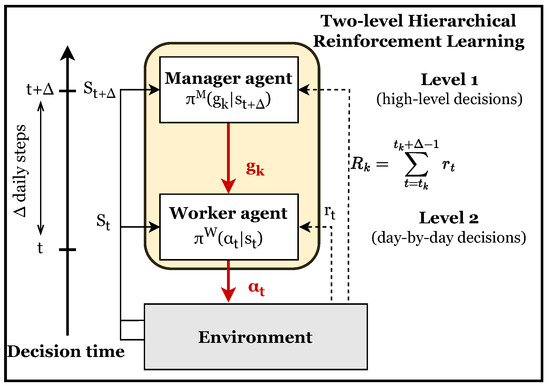
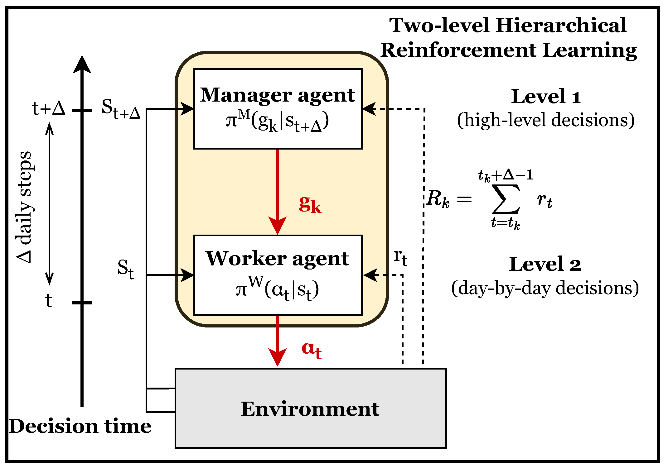
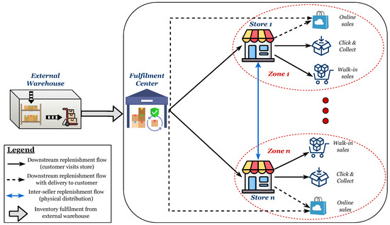
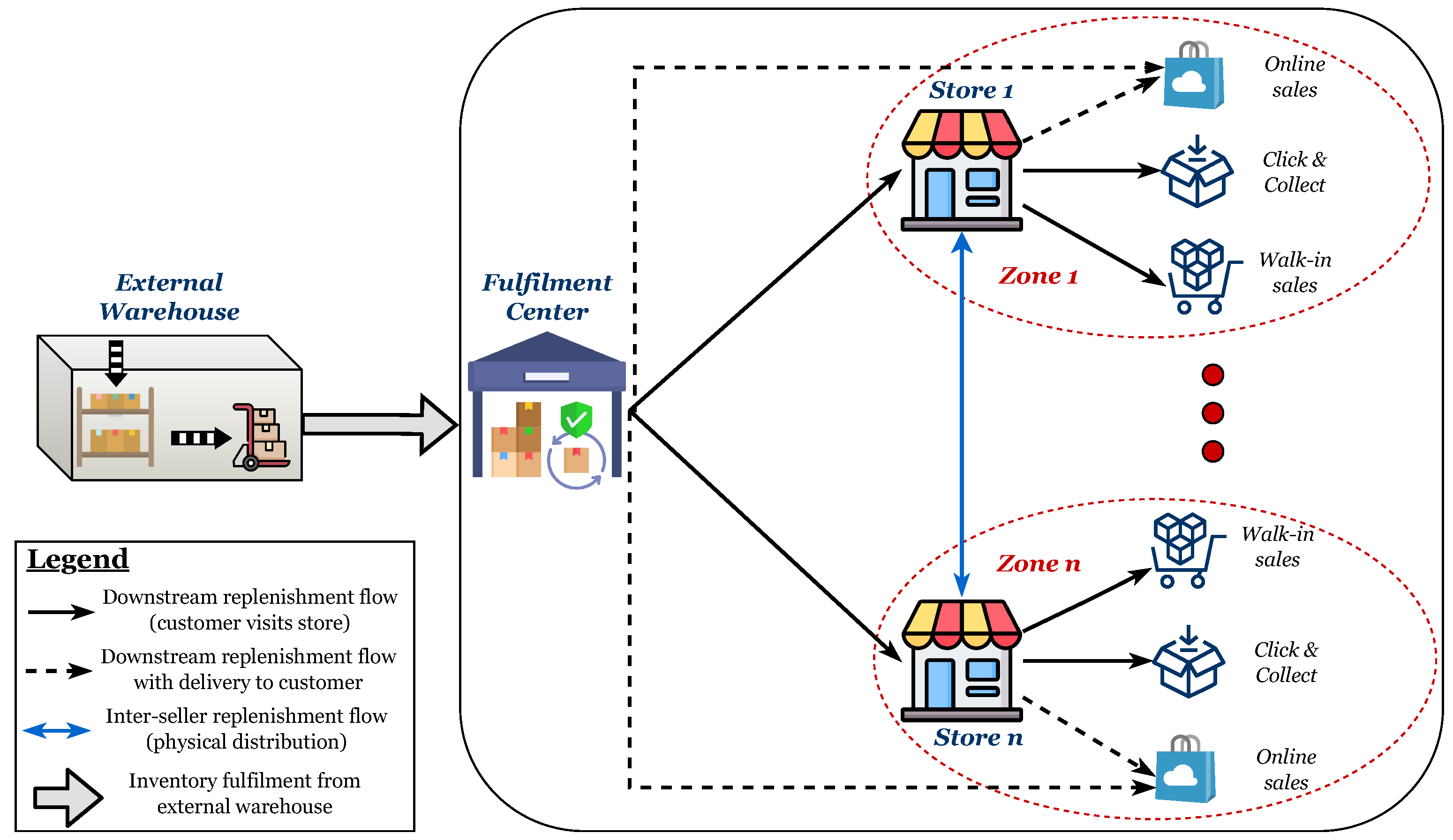
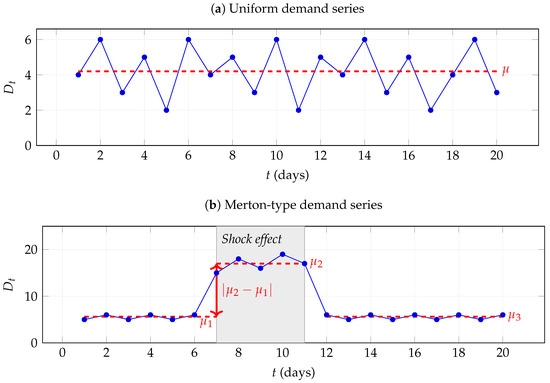
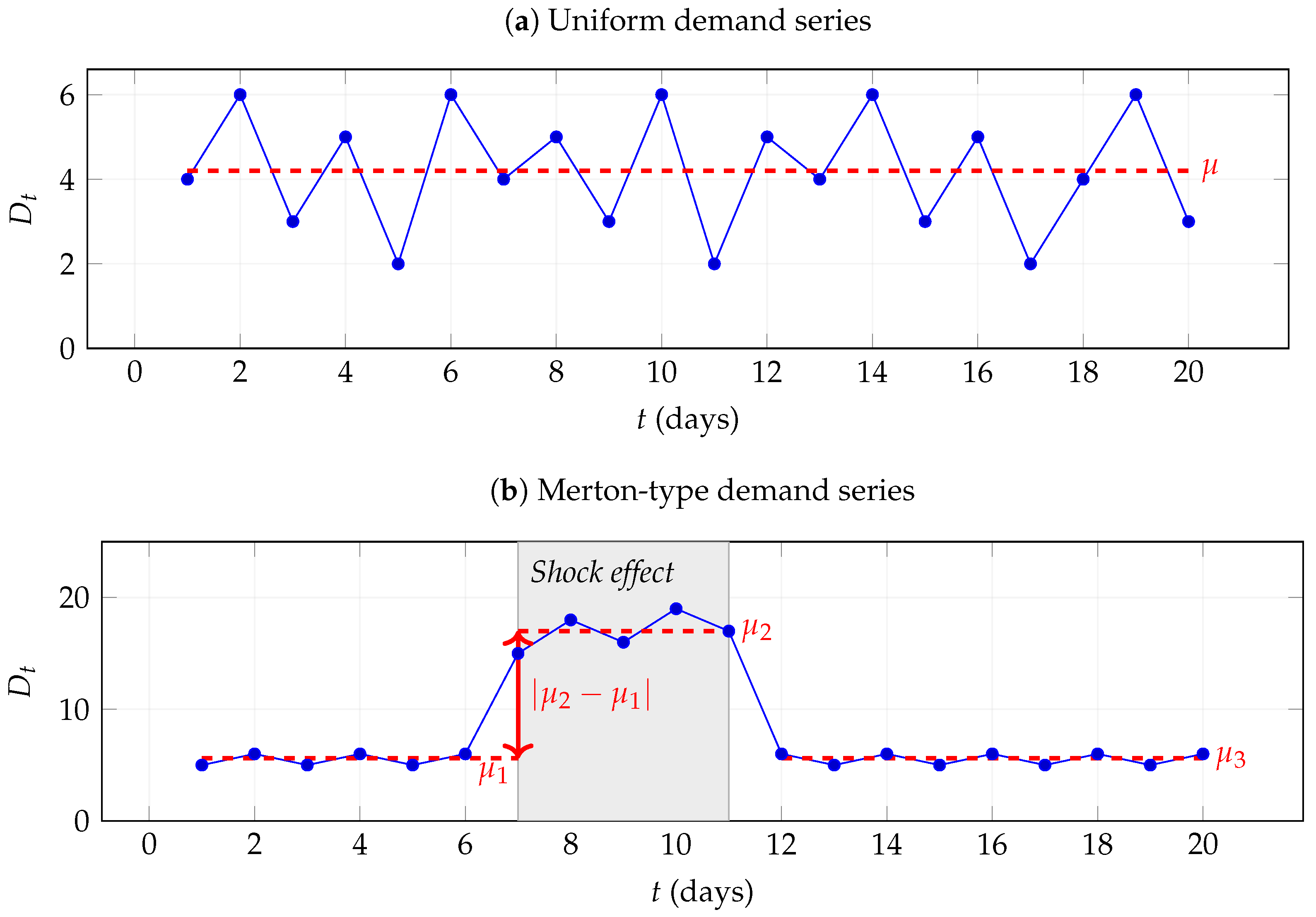
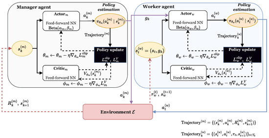
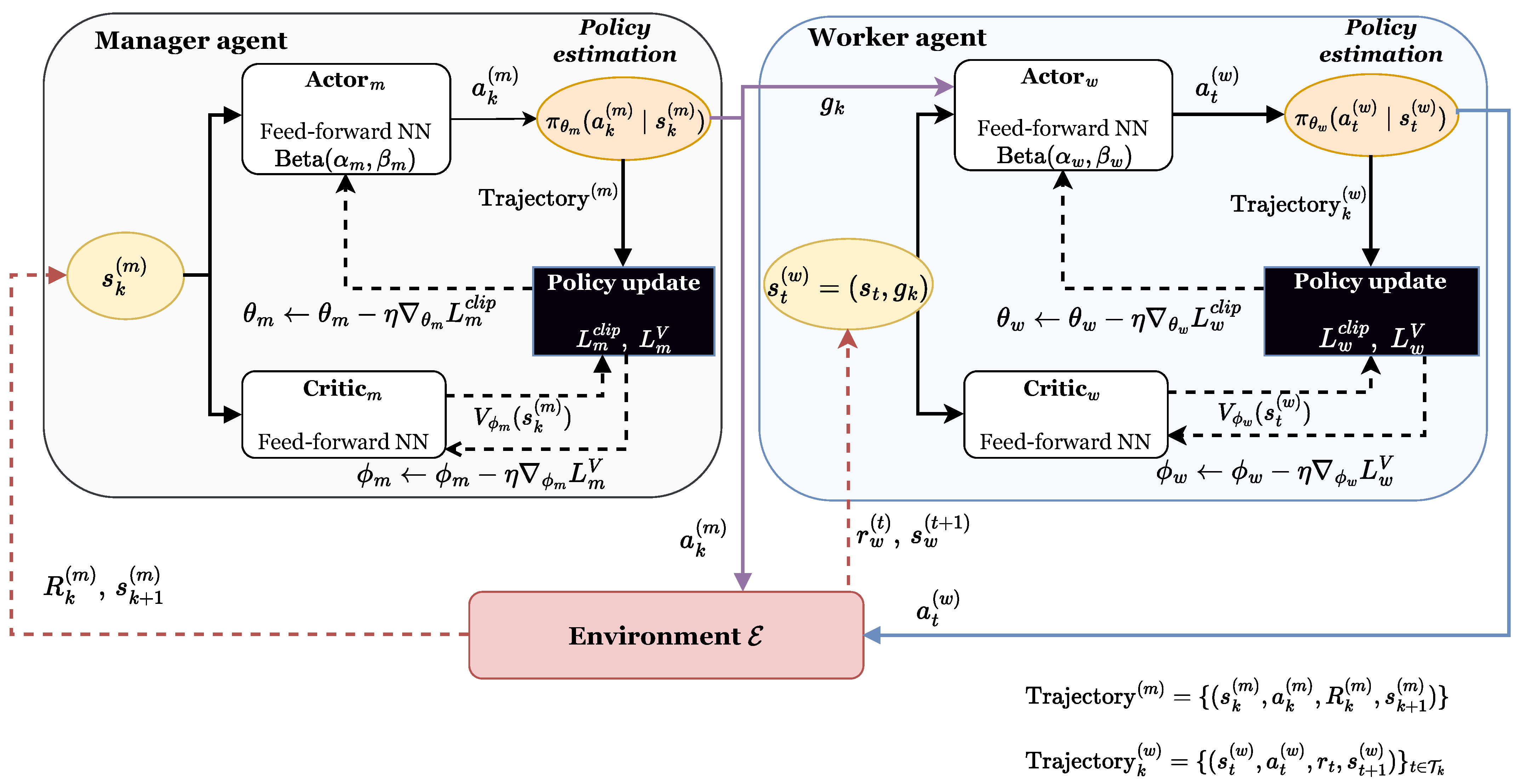
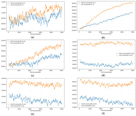
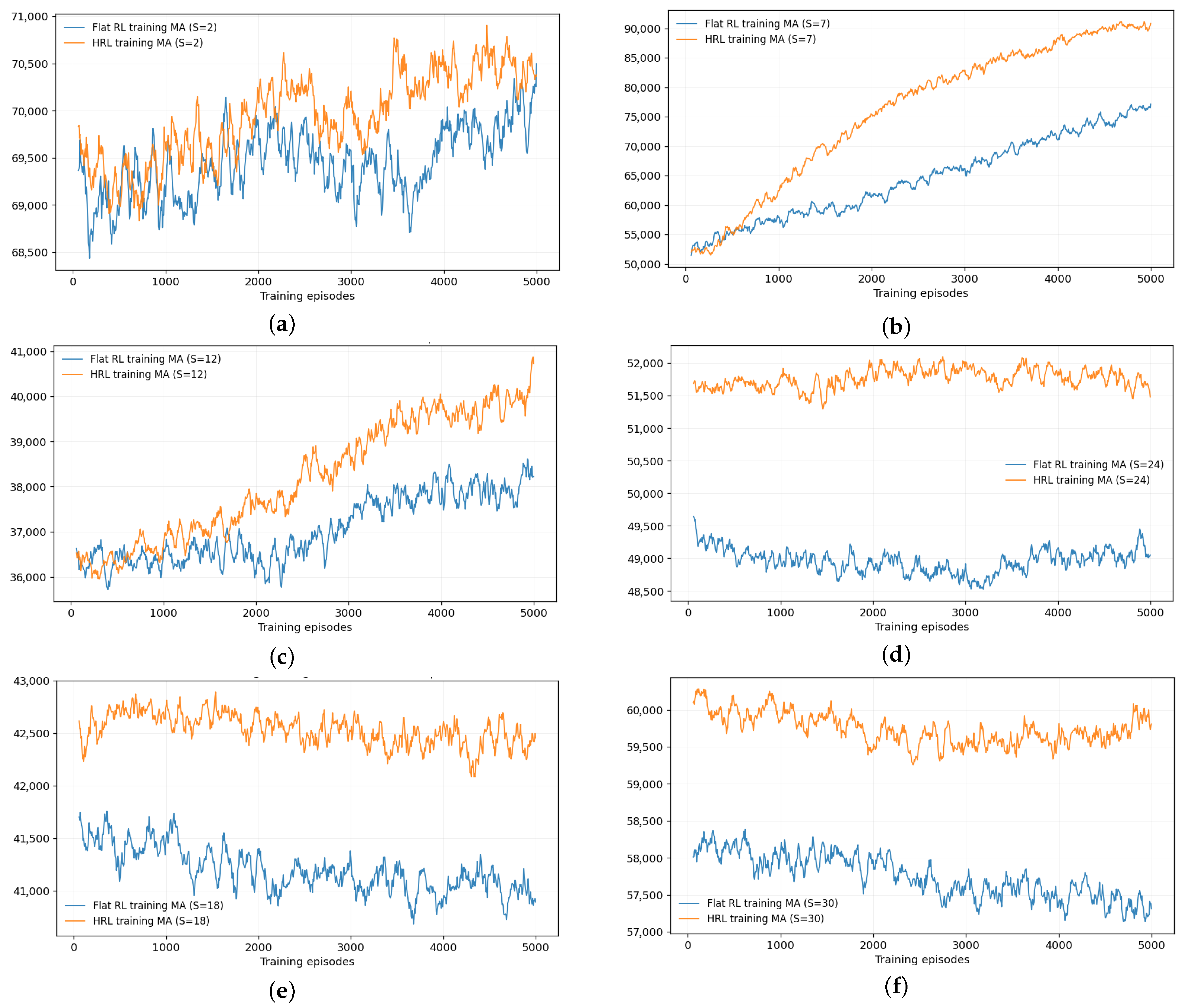
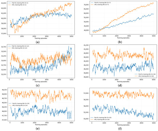
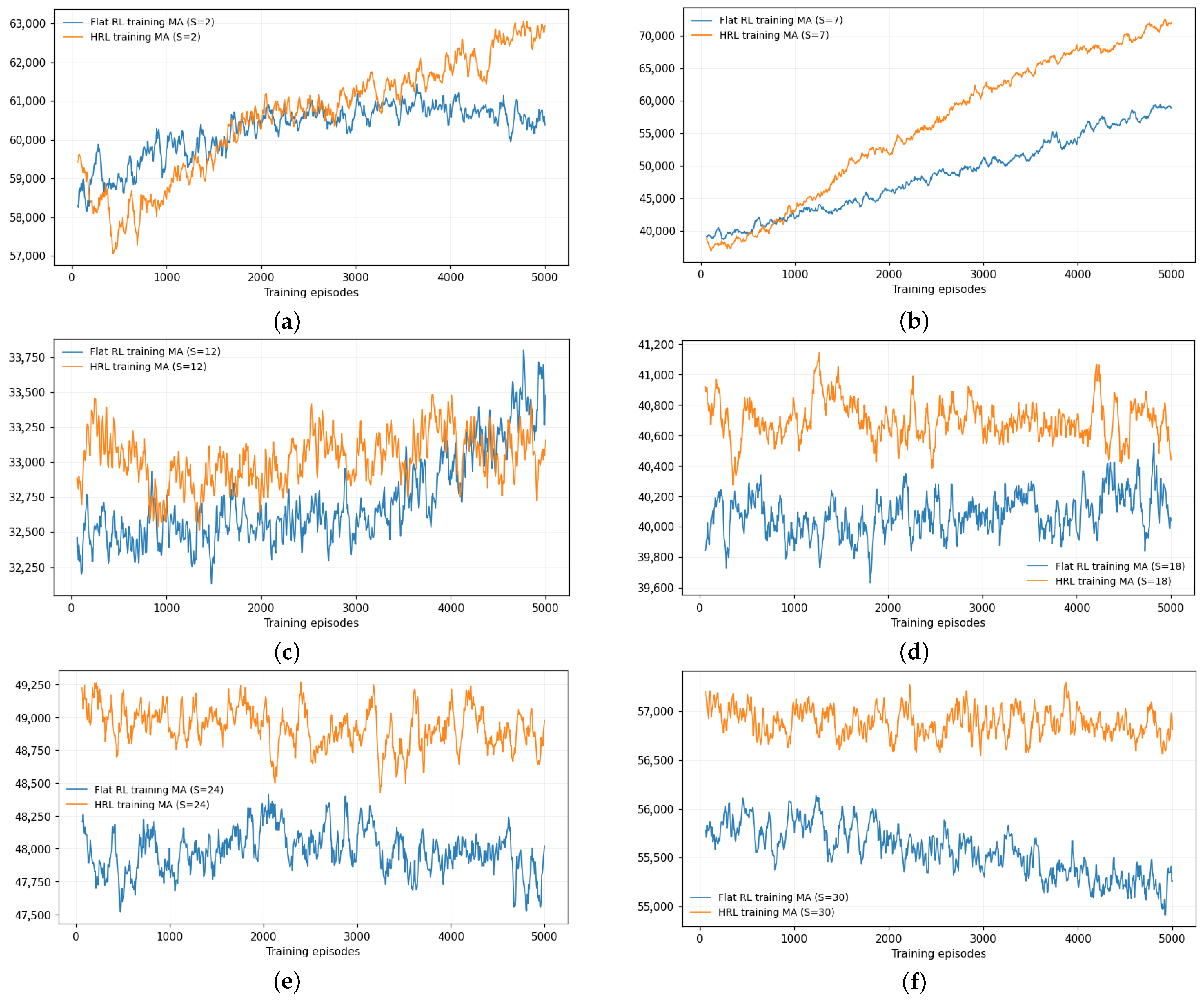
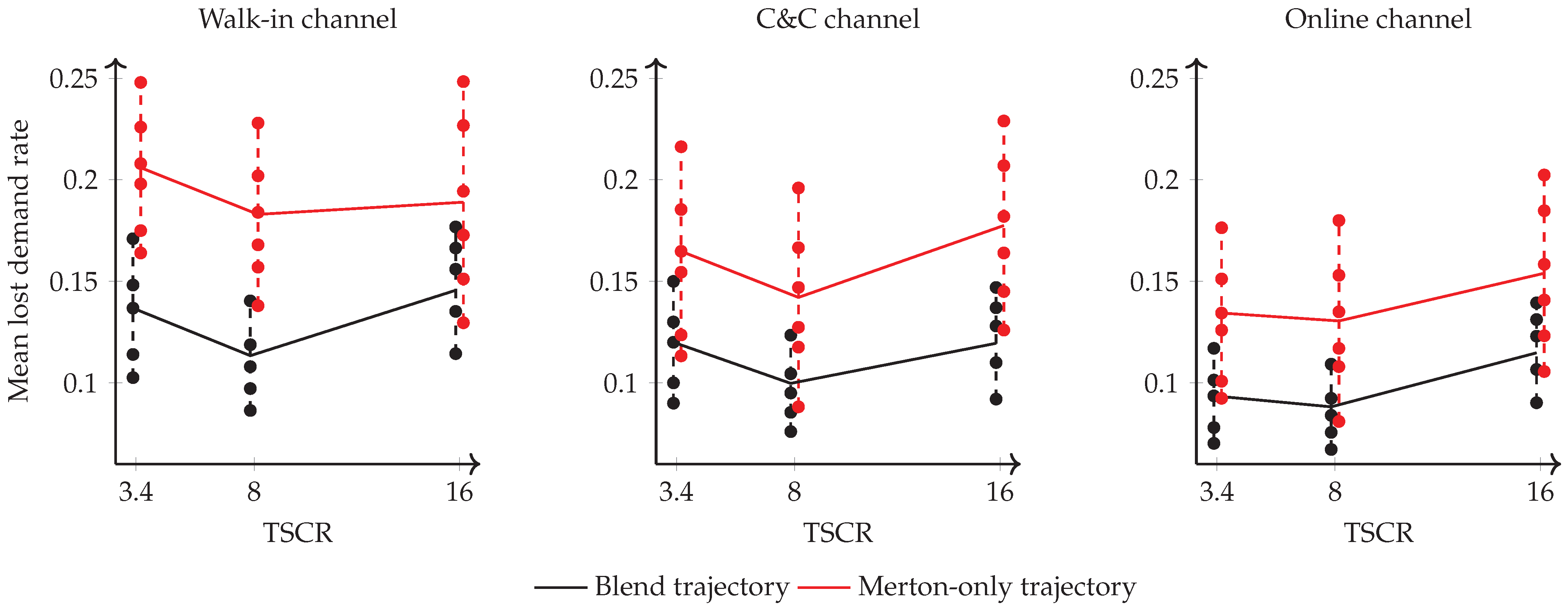

Disclaimer/Publisher’s Note: The statements, opinions and data contained in all publications are solely those of the individual author(s) and contributor(s) and not of MDPI and/or the editor(s). MDPI and/or the editor(s) disclaim responsibility for any injury to people or property resulting from any ideas, methods, instructions or products referred to in the content. |
© 2026 by the authors. Licensee MDPI, Basel, Switzerland. This article is an open access article distributed under the terms and conditions of the Creative Commons Attribution (CC BY) license.