Dynamic Imaging Simulation and Angular Measurement Performance Degradation of Interferometric Star Trackers

Abstract

Interferometric star trackers (ISTs) achieve high-precision angular measurement by encoding the stellar incident direction into multichannel interference phases. Besides image smearing, platform motion continuously changes the interference phase during a finite exposure, an effect not captured by conventional geometric star-image models. However, the quantitative relationship between platform motion characteristics and interferometric measurement degradation, which is essential for dynamic performance assessment and system-level optimization of ISTs, remains insufficiently characterized. We develop a full-link dynamic imaging model that incorporates broadband stellar radiation, multiple synthetic diffraction orders, multichannel energy modulation, exposure integration, and detector noise. The four-channel response is expressed as the temporal mean of a complex interference phasor, whose magnitude and argument define the modulation retention factor and dynamic phase bias, respectively. Static angular scanning experiments yield correlation coefficients above 0.97 between simulated and measured channel responses. Under a locally linear phase-to-angle relationship along the interferometric sensing direction, constant-rate motion produces a sinc response, whereas integer-cycle periodic jitter produces a zeroth-order Bessel response. For noninteger-cycle jitter, the response additionally depends on the exposure-to-jitter period ratio and initial phase. When constant-rate motion and periodic jitter coexist, they modulate the same phasor and produce a generally nonseparable response. Within the investigated parameter range, the maximum absolute difference in modulation retention between the coupled response and the independent sinc–Bessel product reaches approximately 0.58. This peak occurs near a normalized phase sweep of 1 and a normalized jitter-induced phase amplitude of 0.8. The model provides a basis for defining dynamic operating limits and selecting exposure parameters and platform stability requirements for ISTs.

1. Introduction

Star trackers provide inertial attitude references for high-precision spacecraft attitude determination [1,2]. As demands for maneuverability, dynamic range, and update rate data increase, their performance can no longer be assessed solely under static conditions [3]. During a finite exposure, platform motion changes the stellar incident direction and image-plane projection, causing star-image smearing, a reduced signal-to-noise ratio, and degraded centroiding accuracy [4,5]. Physics-based dynamic imaging models therefore provide a practical approach not only for performance prediction and system evaluation when on-orbit disturbances are difficult and costly to reproduce experimentally, but also for establishing quantitative relationships between platform motion characteristics and measurement degradation.

In conventional imaging star trackers, stellar directions are inferred primarily from star-spot positions on the focal plane. Platform motion is therefore modeled through star-image trajectories and the associated redistribution of image energy during exposure. Existing point spread function (PSF) and motion blur models cover constant-rate rotation, three-axis angular motion, variable-rate motion, periodic or random vibration, and combined rotation and vibration [6,7,8,9,10]. These models quantify the resulting degradation in SNR and centroiding accuracy. Although they accommodate increasingly complex motion, the geometric star-spot position remains the fundamental observable for direction determination.

Unlike conventional imaging star trackers, ISTs rely on both geometric and interferometric observables. Small variations in the stellar incident direction can be detected with high sensitivity from changes in the position or phase of interference fringes [11,12,13]. A spatial modulation structure, such as the beam splitter assembly, converts these angular changes into periodic energy variations across multiple measurement channels. The star-spot position provides a coarse angular estimate, whereas the relative channel energies enable interference-phase retrieval for fine measurement. Platform motion therefore affects an IST not only through star-spot displacement but also through the temporal evolution of the angle-dependent interference response during exposure. In contrast to conventional imaging star trackers, where motion-induced degradation can be approximated by convolving a nearly invariant stellar PSF with the image trajectory, the IST response varies with the stellar incident angle because the multichannel interference energies are highly angle dependent. Therefore, finite-exposure integration in an IST represents the accumulation of different interference states rather than merely the spatial redistribution of stellar energy.

Existing studies on ISTs have systematically investigated interferometric angular measurement principles [14,15], optical system design [16], the effects of fabrication and alignment errors [17], and broadband imaging and measurement [18]. Several IST prototypes have been reported [19], and NISTEx-II was launched in May 2019 [20]. The NISTEx-II report gives performance specifications at selected angular rates but does not describe the underlying finite-exposure dynamic-response model. Such specifications do not establish how motion parameters govern modulation retention, dynamic phase bias, or the effects of coupled motion. Our previous broadband phase-compensation static model [18] established the static relationship between incident angle, multichannel energy distribution, and retrieved phase. It does not, however, quantify how finite-exposure motion changes this response or whether coexisting motion components can be treated independently.

Here, we extend this model to full-link dynamic imaging by integrating the time-varying interference response over each exposure while retaining the broadband optical and detector processes. The magnitude and argument of a normalized complex interference factor define modulation retention and dynamic phase bias, respectively. Under local phase linearization, we derive analytical responses for constant-rate motion, periodic attitude jitter, and their combination to assess the limitations of the independent sinc–Bessel product. We compare simulated channel responses with static angular scanning measurements and evaluate dynamic angular measurement performance through noise-inclusive simulations. The framework supports model-based assessment of dynamic operating limits, exposure selection, and platform stability requirements.

2. System Configuration and Operating Principle

2.1. System Configuration

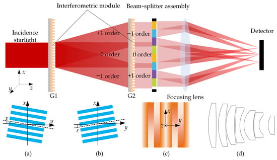
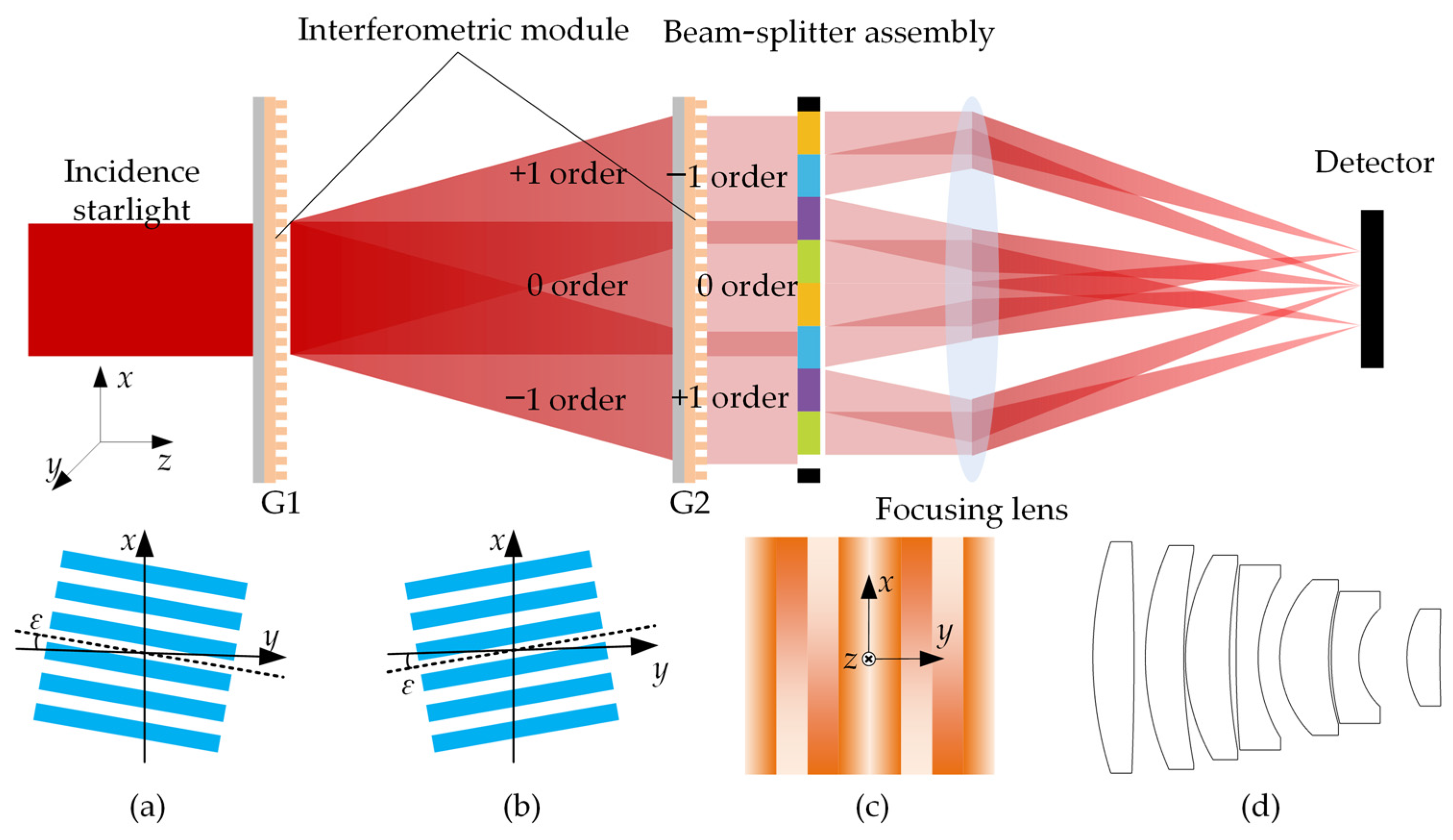
Figure 1 shows the IST optical configuration. The IST comprises an interferometric module, a beam splitter assembly, a focusing lens, and a detector. The interferometric module contains two parallel phase Ronchi gratings, G1 and G2, with a common period p and axial separation z. Their grating lines are oriented at +ε and −ε relative to the y-axis, generating a spatially modulated moiré interference field. Starlight passing through both gratings forms multiple synthetic diffraction orders, whose path-dependent phase differences encode the incident direction.

Figure 1. Optical configuration of the IST and component geometries. The upper schematic shows the optical path from incident starlight through the interferometric module, beam splitter assembly, and focusing lens to the detector. (a,b) In-plane orientations of phase Ronchi gratings G1 and G2, respectively; (c) thickness profile of the beam splitter assembly along the optical axis, where the color gradient represents the relative thickness variation; (d) focusing lens configuration.

Located downstream of G2, the beam splitter assembly contains eight rectangular optical wedge subapertures arranged along the y-direction. Each subaperture samples a local region of the interference field and deflects the sampled light toward a designated detector region. The subapertures are paired to form four phase measurement channels. After focusing, the interference phase is retrieved from the relative energies integrated over the four star-spot regions.

2.2. Synthetic Diffraction Orders and Stellar Interference Phase

Let $m$ and $m^{\prime }$ denote the diffraction orders generated by G1 and G2, respectively. Retaining only the 0 and ±1 orders of each grating, the synthetic diffraction order is defined as follows:

$$M=m+m^{\prime }.$$

(1)

Retaining the 0 and ±1 diffraction orders, the synthetic zeroth-order interference is mainly formed by the coherent superposition of three propagation paths [18]. The phase difference between the (+1, −1) and (−1, +1) diffraction paths carries the fine angular information. The (0, 0) path mainly contributes to the common intensity component.

Let α and β denote the incident angles along the interferometric sensing direction and its orthogonal direction, respectively. For a small grating-line angle, the differential phase can be approximated as [16]:

$$\phi \left(\alpha \right)\approx {\phi }_0-{\displaystyle \frac{4\pi z}{p}}\sin \alpha ,$$

(2)

where φ₀ is the fixed phase offset introduced by the system. The stellar interference phase used for angular measurement is then defined as follows:

$$\tilde{\phi }\left(\alpha \right)=\phi \left(\alpha \right)-{\phi }_0\approx -{\displaystyle \frac{4\pi z}{p}}\sin \alpha ,$$

(3)

Under the adopted phase approximation, the direct contribution of β is neglected, and the reduced-order phase model depends on α. The orthogonal angular component β is still retained in the full-link imaging model because it affects the stellar image position and channel energy distribution. Therefore, the subsequent reduced-order dynamic analysis represents the dominant phase evolution by mapping the time-varying sensing-axis angle $\alpha \left(t\right)$ to the corresponding interference phase $\phi \left(t\right)$.

2.3. Four-Channel Phase-Shifting Measurement and Wrapped-Phase Retrieval

The beam splitter assembly divides the local interference field among four simultaneous measurement channels with fixed relative phase shifts. Under ideal conditions, the integrated channel energies, I₁–I₄, are [18]:

$$I_k=A+B\cos \left(\tilde{\phi }+{\delta }_k\right),\hspace{1em}k=1,2,3,4,$$

(4)

where A is the common DC component, B is the interference modulation amplitude, and ${\delta }_k$ is the fixed phase shift of channel k. Adjacent channels in the ideal four-channel configuration differ by $\pi /2$.

Differencing the four channel responses removes the common DC component and yields two quadrature observables. The wrapped phase is then:

$${\tilde{\phi }}_w=\arctan \left({\displaystyle \frac{I_4-I_2}{I_1-I_3}}\right).$$

(5)

Because the arctangent is periodic, Equation (5) returns only the principal value in $\left(-\pi /2,\pi /2\right)$, leaving an integer-cycle ambiguity.

Equivalently, the four-channel response defines the complex differential observable:

$$Z=\left(I_1-I_3\right)+\mathrm{j}\left(I_4-I_2\right).$$

(6)

Under ideal conditions, it reduces to:

$$Z=2B\exp \left(\mathrm{j}\tilde{\phi }\right).$$

(7)

This complex form underpins the dynamic exposure model in Section 4. During platform motion, the instantaneous complex interference phasor evolves continuously, and the detector records the exposure-integrated complex differential signal.

2.4. Absolute Phase Recovery and High-Precision Angular Inversion

The wrapped phase from (5) is related to the absolute phase by:

$${\tilde{\phi }}_{\mathrm{abs}}={\tilde{\phi }}_w+2\pi N,N\in \mathbb{Z},$$

(8)

where N is the unknown phase-cycle index.

To resolve the integer-cycle ambiguity, the geometric image positions of the star spots on the detector are used to obtain a coarse estimate of the stellar incident direction. During system design and calibration, the mapping relationships among the wedge deflection angles, focal length, image-plane positions, and incident direction are predetermined. Therefore, the centroid positions of the four star spots can be used to obtain coarse angular estimates along the interferometric sensitive direction and its orthogonal direction. Once the phase-cycle index N is determined, the absolute interference phase is recovered using (8), and the high-precision incident angle along the interferometric sensitive direction is subsequently obtained by inverting the phase-to-angle mapping relationship.

Under ideal phase retrieval, unambiguous cycle selection requires a coarse angular estimation error below half of the local angular phase period. Therefore, the allowable coarse estimation error can be expressed as [16]:

$$\Delta \alpha \le {\displaystyle \frac{p}{4z}}.$$

(9)

Equation (9) constrains the coarse angular estimation error rather than the total star-spot displacement during exposure.

The incident angle along the orthogonal direction is primarily determined from the geometric positions of the star spots. This establishes a two-stage angular measurement scheme combining geometric-position-based coarse measurement with interference-phase-based fine measurement: geometric imaging provides large-range, unambiguous angular information, whereas the interference phase enables high-sensitivity angular discrimination within a single phase cycle. This measurement scheme also provides the basis for analyzing phase-branch failure under dynamic conditions in the subsequent sections.

3. Full-Link Imaging Model

This section maps stellar directions and radiative properties, together with platform attitude, to the detector’s finite-exposure digital output. Unlike conventional trackers, an IST produces wavelength-, synthetic-order-, and channel-dependent image positions and energies for each star. The full-link imaging model therefore combines time-varying direction projection, multiple synthetic diffraction orders, multichannel energy modulation, optical spreading, exposure integration, and detector noise.

3.1. Coordinate Transformation Model

The inertial star vectors are transformed into the tracker coordinate system using the time-dependent attitude matrix. The corresponding incident angles and image-plane positions of wavelength- and synthetic-order-dependent components are then calculated as:

$$\left\{\begin{array}{l}{X}_{i,l,M,k}\left(t\right)=f\tan \left(\arcsin \left(\sin {\alpha }_i\left(t\right)+{\displaystyle \frac{M{\lambda }_l}{p}}\right)+{\theta }_{x,k}\right)\\ Y_{i,l,M,k}\left(t\right)=f\tan \left({\beta }_i\left(t\right)+{\theta }_{y,k}\right)\end{array}\right.,$$

(10)

where ${\lambda }_l$ is the lth sampled wavelength; f is the focal length of the focusing lens; and ${\theta }_{x,k}$ and ${\theta }_{y,k}$ are the equivalent deflection angles of the kth beam-splitting channel along the two orthogonal directions, respectively.

For M = 0, the output direction contains no wavelength-dependent synthetic-order deflection, making the ideal star-point center insensitive to wavelength. For M ≠ 0, wavelength-dependent output directions produce a dispersed broadband distribution.

Thus, a single star produces a set of image points indexed by wavelength, synthetic diffraction order, measurement channel, and instantaneous incident direction:

$${{\rm P}}_i\left(t\right)=\left\{X_{i,l,M,k}\left(t\right),Y_{i,l,M,k}\left(t\right)\right\}.$$

(11)

During exposure, the time-dependent attitude transformation produces continuous trajectories of all synthetic diffraction components. The field-of-view screening therefore considers the full motion range, along with beam-splitting deflections and wavelength-dependent dispersion, rather than only the nominal zero-order position.

3.2. Energy Conversion Model

Energy conversion proceeds from stellar irradiance to channel-resolved photoelectron rates. The apparent magnitude and spectrum determine broadband irradiance at the entrance pupil. The interferometric module and beam splitter assembly then distribute this energy across wavelengths, synthetic diffraction orders, and measurement channels before detector conversion.

The operating spectral range is discretized into $N_{\lambda }$ wavelength intervals. Based on the magnitude–irradiance relation [8], the irradiance contribution of the ith star in the lth wavelength interval can be calculated as:

$$E_{i,l}=E_{\mathrm{ref}}{10}^{-0.4\left(m_i-m_{\mathrm{ref}}\right)}{w}_{i,l},$$

(12)

where m_i is the apparent magnitude of the ith star; m_ref and E_ref are the apparent magnitude of the reference star and the corresponding reference irradiance, respectively; and w_i,l is the normalized spectral weight determined from the stellar effective temperature and spectral type.

For each star, wavelength interval, wedge subaperture, and synthetic diffraction order, the optical power after propagation through the interferometric module is calculated by considering the incident stellar amplitude, diffraction coefficients of the phase gratings, propagation phase between optical elements, effective aperture distribution, and subaperture position [18]:

$$P_{i,l,M,n}\left(t\right)={\displaystyle \frac{c{\epsilon }_0}{2}}{\displaystyle \iint {\left|{\displaystyle \sum _{m+m^{\prime }=M}{A}_{i,l,m,m^{\prime },n}\left(f_x,f_y,t\right)}\right|}^2\mathrm{d}{f}_x\mathrm{d}{f}_y}$$

(13)

where c is the speed of light in vacuum, and ${\epsilon }_0$ is the vacuum permittivity.

The eight wedge subapertures are paired into the four measurement channels defined in Section 2. The total power of order M in channel k is:

$$P_{i,l,M,k}\left(t\right)=P_{i,l,M,k}^{\left(1\right)}\left(t\right)+P_{i,l,M,k}^{\left(2\right)}\left(t\right),k=1,2,3,4,$$

(14)

where $P^{\left(1\right)}$ and $P^{\left(2\right)}$ represent the contributions from the two paired wedge subapertures, respectively. Considering the detector quantum efficiency $\eta \left({\lambda }_l\right)$, the corresponding photoelectron generation rate is expressed as:

$${\dot{N}}_{i,l,M,k}\left(t\right)=P_{i,l,M,k}\left(t\right){\displaystyle \frac{{\lambda }_l\eta \left({\lambda }_l\right)}{hc}},$$

(15)

where h is Planck’s constant.

Each synthetic diffraction component is spatially distributed using a normalized PSF obtained from the full optical system model at the nominal field position. The PSF is normalized to a unit integral and held fixed in shape, while the model retains time-varying image positions and interference energies. Field- and wavelength-dependent PSF variations may alter the energy captured within finite channel integration regions and thereby affect phase retrieval. The dynamic impact of these PSF-shape variations is not quantified here. The instantaneous photoelectron generation-rate distribution of the ith star is then expressed as:

$$K_i\left(X,Y,t\right)={\displaystyle \sum _{l=1}^{N_{\lambda }}{\displaystyle \sum _{M\in {\mathcal{M}}_i\left(t\right)}{\displaystyle \sum _{k=1}^4{\dot{N}}_{i,l,M,k}\left(t\right)h_{\mathrm{PSF}}\left(X-X_{i,l,M,k}\left(t\right),Y-Y_{i,l,M,k}\left(t\right)\right)}}},$$

(16)

where ${\mathcal{M}}_i\left(t\right)$ denotes the set of effective synthetic diffraction orders that can propagate under the current incident direction and operating spectral range and contribute to the detector response.

Different stars lack a stable mutual phase and therefore add incoherently at the photoelectron-rate level. The instantaneous distribution for the complete star field can be expressed as:

$$R\left(X,Y,t\right)={\displaystyle \sum _{i=1}^{N_s}{K}_i\left(X,Y,t\right)}+R_{\mathrm{bg}}\left(X,Y,t\right),$$

(17)

where $R_{bg}\left(X,Y,t\right)$ denotes the equivalent photoelectron generation-rate distribution on the detector due to sky background radiation and system stray light.

For each detector pixel $\left(u,v\right)$ and exposure time T_e, the expected stellar-signal and background electron counts are:

$$\left\{\begin{array}{l}{\mu }_{uv}^{\mathrm{sig}}={\displaystyle {\int }_0^{T_e}{\displaystyle {\iint }_{{\Omega }_{uv}}{\displaystyle \sum _{i=1}^{N_s}{K}_i\left(X,Y,t\right)\mathrm{d}X\mathrm{d}Y\mathrm{d}t}}}\\ {\mu }_{uv}^{\mathrm{bg}}={\displaystyle {\int }_0^{T_e}{\displaystyle {\iint }_{{\Omega }_{uv}}{R}_{\mathrm{bg}}\left(X,Y,t\right)\mathrm{d}X\mathrm{d}Y\mathrm{d}t}}\end{array}\right.$$

(18)

Equation (18) integrates the time-varying photoelectron rate over both the pixel area and exposure. Platform motion changes image positions and channel energies simultaneously. Dynamic IST imaging cannot be represented by translating a fixed static intensity template along the star trajectory because both the diffraction component positions and the channel-dependent energies vary during exposure.

3.3. Noise Model and Digital Image Generation

The detector noise model includes photon shot noise, dark-current noise, readout noise, and ADC quantization effects. These noise sources are modeled according to standard detector noise formulations. Considering the stellar signal, background signal, and dark current, the generated electron number of each pixel during one exposure is modeled as:

$$N_{uv}\sim \mathrm{Poisson}\left({\mu }_{uv}^{\mathrm{sig}}+{\mu }_{uv}^{\mathrm{bg}}+{\mu }_{uv}^{\mathrm{dark}}\right)$$

(19)

where ${\mu }_{uv}^{\mathrm{sig}}$, ${\mu }_{uv}^{\mathrm{bg}}$, and ${\mu }_{uv}^{\mathrm{dark}}$ denote the expected electron counts from the stellar signal, background radiation, and dark current, respectively.

The readout noise introduced during electron conversion is modeled as a zero-mean Gaussian process:

$$n_{uv}^{\mathrm{read}}\sim \mathcal{N}\left(0,{\sigma }_{\mathrm{read}}^2\right),$$

(20)

where ${\sigma }_{\mathrm{read}}$ is the standard deviation of the readout noise.

After gain conversion and ADC quantization, the digital output of each pixel is obtained as:

$$D_{uv}=\mathcal{Q}\left(N_{uv}+n_{uv}^{\mathrm{read}}\right)$$

(21)

where $\mathcal{Q}\left(\cdot \right)$ denotes the quantization function, including the gain conversion from electron count to digital number (DN), the effective quantization bit depth, and saturation clipping.

The full-link imaging model therefore maps inertial stellar positions and stellar spectra to digital interferometric star images. It includes synthetic-order propagation, beam splitter energy modulation, optical imaging, finite-exposure integration, and detector noise. Section 5 uses this model to simulate motion-dependent images and evaluate the dynamic angular measurement degradation model developed in Section 4.

4. Dynamic Angular Measurement Performance Degradation Model

The full-link imaging model in Section 3 describes dynamic interferometric star-image formation under platform motion. However, its coupled optical and detector processes obscure the direct dependence of angular measurement performance on motion parameters. We therefore derive a reduced-order four-channel model for the target synthetic zeroth order. Finite exposure is represented as the temporal average of a time-varying complex interference phasor. This model is used to analyze modulation loss, dynamic phase bias, and angular measurement degradation under constant-rate angular motion, periodic attitude jitter, and their combined effect.

4.1. Dynamic Interference Response Model

When the platform undergoes attitude motion, the stellar incident angle along the interferometric sensitive direction changes from a static quantity to a time-varying function $\alpha \left(t\right)$. Let $C=4\pi z/p$, and the corresponding interference phase can be expressed as:

$$\tilde{\phi }\left(t\right)\approx -C\sin \alpha \left(t\right),$$

(22)

Equation (22) retains the nonlinear dependence on the sensing-axis angle. Local linearization is introduced in Section 4.2 to obtain closed-form motion responses.

For analytical treatment, we evaluate the target synthetic zeroth-order response at the central wavelength. We assume the four-channel common component and static modulation amplitude are constant during one exposure. Using the phase-shifting relation in Section 2.3, the instantaneous photoelectron generation rate in channel k can be expressed as:

$$J_k\left(t\right)=A_0+B_0\cos \left(\tilde{\phi }\left(t\right)+{\delta }_k\right),k=1,2,3,4,$$

(23)

where A₀ and B₀ denote the common DC component and the static modulation amplitude, respectively, and ${\delta }_k$ is the fixed phase shift of the kth channel.

The exposure interval is centered at the midpoint of the integration window, and therefore the integration limits are selected as $\left[-T_e/2,T_e/2\right]$, which is equivalent to the conventional $\left[0,T_e\right]$ definition after a time origin shift. The integrated response of the kth channel over a single exposure is then:

$${\overline{J}}_k={\displaystyle {\int }_{-T_e/2}^{T_e/2}{J}_k\left(t\right)\mathrm{d}t.}$$

(24)

The four-channel exposure-integrated responses can be combined as:

$$Z=\left({\overline{J}}_1-{\overline{J}}_3\right)+\mathrm{j}\left({\overline{J}}_4-{\overline{J}}_2\right).$$

(25)

Substituting the instantaneous four-channel responses into the above expression yields the exposure-integrated complex differential signal:

$$Z=2B_0{\displaystyle {\int }_{-T_e/2}^{T_e/2}\exp \left(\mathrm{j}\tilde{\phi }\left(t\right)\right)\mathrm{d}t.}$$

(26)

Let the interference phase corresponding to the incident angle ${\alpha }_c$ at the nominal trajectory center be ${\tilde{\phi }}_c=-C\sin {\alpha }_c$. For constant-rate motion, this reference coincides with the mid-exposure angle. Based on the exposure-integrated complex differential signal, we define a normalized dynamic interference factor to quantify the motion-induced degradation of interferometric measurement:

$$\Gamma ={\displaystyle \frac{1}{T_e}}{\displaystyle {\int }_{-T_e/2}^{T_e/2}\exp \left(-\mathrm{j}C\left(\sin \alpha \left(t\right)-\sin {\alpha }_c\right)\right)\mathrm{d}t.}$$

(27)

The exposure-integrated complex differential observable can then be written as $Z=2B_0{T}_e\Gamma \exp \left(j{\tilde{\phi }}_c\right).$ Accordingly, the modulation retention factor and dynamic phase bias are defined as:

$${\rho }_m=\left|\Gamma \right|,\Delta {\tilde{\phi }}_d=\arg \left(\Gamma \right).$$

(28)

The corresponding exposure-equivalent interference phase is:

$${\tilde{\phi }}_e={\tilde{\phi }}_c+\Delta {\tilde{\phi }}_d.$$

(29)

The dynamic interference factor $\Gamma$ is the key quantity characterizing finite-exposure dynamic effects. Its magnitude represents the fraction of the effective interference modulation retained after exposure relative to the static state, whereas its argument represents the equivalent phase shift induced by exposure integration. Thus, the dynamic interference factor characterizes an arbitrary platform attitude trajectory via the corresponding time-varying interference phase.

4.2. Interference Responses Under Typical Platform Motions

We analyze constant-rate angular motion, periodic attitude jitter, and their combination along the interferometric sensing direction. As assumed in Section 4.1, the common DC component and static modulation amplitude remain constant during each exposure. Cross-axis effects that change channel energy collection, such as aperture clipping or cross-channel leakage, are not characterized by these reduced-order expressions. The following closed-form responses rely on local linearization of the phase–angle relationship, with the corresponding conditions specified below.

4.2.1. Constant-Rate Angular Motion

Assume that, during a single exposure, the line-of-sight angle along the sensitive direction varies at a constant angular rate:

$$\alpha \left(t\right)={\alpha }_c+{\omega }_{\alpha }t,$$

(30)

where ${\alpha }_c$ is the line-of-sight angle at the midpoint of the exposure, and ${\omega }_{\alpha }$ is the equivalent angular rate along the sensitive direction. Substituting (30) into the definition of the dynamic interference factor gives the exact response under constant-rate angular motion:

$${\Gamma }_u={\displaystyle \frac{1}{T_e}}{\displaystyle {\int }_{-T_e/2}^{T_e/2}\exp \left[-\mathrm{j}C\left(\sin \left({\alpha }_c+{\omega }_{\alpha }t\right)-\sin {\alpha }_c\right)\right]\mathrm{d}t.}$$

(31)

Equation (31) gives the dynamic interference response under constant-rate angular motion. However, because the interference phase depends nonlinearly on the incident angle through a sinusoidal relationship, the integral cannot in general be expressed in a simple closed form. To obtain an analytical relationship among the angular rate, exposure time, and dynamic modulation depth, the phase function is expanded in a Taylor series about the midpoint of the exposure:

$$\tilde{\phi }\left(t\right)-{\tilde{\phi }}_c=-C\cos {\alpha }_c{\omega }_{\alpha }t+{\displaystyle \frac{C}{2}}\sin {\alpha }_c{\omega }_{\alpha }^2{t}^2+\mathcal{O}\left({\omega }_{\alpha }^3{t}^3\right).$$

(32)

The phase-to-angle sensitivity at the exposure midpoint is defined as:

$$K_{\alpha }={\left.{\displaystyle \frac{\partial \tilde{\phi }}{\partial \alpha }}\right|}_{{\alpha }_c}=-C\cos {\alpha }_c.$$

(33)

When the second-order phase contribution remains negligible compared with the first-order phase variation over the exposure interval, i.e.,

$$\left|{\displaystyle \frac{\frac{C}{2}\sin {\alpha }_c{\omega }_{\alpha }^2{\left(\frac{T_e}{2}\right)}^2}{C\cos {\alpha }_c{\omega }_{\alpha }\left(\frac{T_e}{2}\right)}}\right|={\displaystyle \frac{\left|\tan {\alpha }_c\right|}{4}}{\omega }_{\alpha }{T}_e\ll 1,$$

(34)

the phase–angle relationship can be locally linearized as:

$$\tilde{\phi }\left(t\right)-{\tilde{\phi }}_c\approx K_{\alpha }{\omega }_{\alpha }t.$$

(35)

For the constant-rate simulations in Section 5.4.1, the maximum angular displacement during a 40 ms exposure is approximately 1.0 × 10⁻³ rad. The detector dimensions and focal length in Table 1 give a larger nominal half-field angle of approximately 4.01°. For midpoint angles within ±4.01°, the ratio in (34) remains below approximately 1.8 × 10⁻⁵, supporting the local phase linearity approximation. Substituting (35) into the dynamic interference factor yields the closed-form response:

$${\Gamma }_v\approx \sin \mathrm{c}\left({\displaystyle \frac{K_{\alpha }{\omega }_{\alpha }{T}_e}{2}}\right).$$

(36)

Table 1. Optical and detector parameters of the IST prototype.

Category	Parameter	Value	Unit
Interferometric Module	Grating Period, p	50	μm
	Grating Separation, z	50	mm
	Grating Groove Angle, ε	0.024	°
Beam Splitter Assembly	Wedge Dimensions, a × b	60 × 7.5	mm × mm
	Deflection Angles, θx1, θx2, θx3, θx4, θy1, θy2, θy3, θy4	0.2, 0, −0.2, 0; 0, 0.2, 0, −0.2	°
Focusing Lens	Focal Length, f	89.1	mm
	PSF	ZEMAX output	—
Detector	Pixel Number, Nx × Ny	1280 × 1024	—
	Pixel Size, dpix	9.76	μm
	Peak Quantum Efficiency, Q	89@610 nm	%
	Exposure Time, Te	40	ms
	Full Well Capacity, NFW	48,000	e−
	Dark Current, id	0.08@−28 °C	e−/s/pixel
	Readout Noise, σr	1.6	e−
	ADC Resolution, nADC	12	bit

The normalized phase sweep over the exposure is defined as:

$$\eta ={\displaystyle \frac{K_{\alpha }{\omega }_{\alpha }{T}_e}{2\pi }},$$

(37)

Accordingly, the modulation retention factor under constant-rate angular motion is ${\rho }_u=\left|\sin \mathrm{c},\left(\pi \eta \right)\right|$. This result shows that, under the local phase linearity condition, the dynamic response to constant-rate angular motion is determined solely by the total phase sweep over the exposure. Within the first positive-response interval, a larger phase sweep strengthens phasor cancellation and reduces modulation retention.

Before the first zero of the sinc response, the dynamic interference factor is real and positive, and the exposure-equivalent phase equals the mid-exposure phase. Near the zero, modulation loss reduces phase observability and increases sensitivity to noise. In the negative sidelobe, the response magnitude recovers, but its sign reversal introduces an equivalent phase shift of approximately π. The simulations in Section 5 use static phase-to-angle inversion without motion state information or dynamic phase-branch correction. Under this estimation scheme, the reversed response can produce phase-branch misidentification and systematic angular bias. The performance of phase tracking and dynamic compensation is not evaluated here.

The sinc response relies on local linearization of the phase-angle relation. When the angular displacement becomes large, higher-order phase terms are no longer negligible, and the exact response must be evaluated from (31). In this regime, even constant-rate motion can produce a complex dynamic interference factor and additional dynamic phase bias.

4.2.2. Periodic Attitude Jitter

Assume that the platform undergoes single-frequency periodic attitude jitter along the interferometric sensitive direction:

$$\alpha \left(t\right)={\alpha }_c+a_{\alpha }\sin \left(w_{j}t+\psi \right),$$

(38)

where $a_{\alpha }$, $w_j$, and $\psi$ denote the angular jitter amplitude, angular frequency, and initial phase, respectively. Substituting (38) into the definition of the dynamic interference factor gives the exact response under periodic attitude jitter:

$${\Gamma }_j={\displaystyle \frac{1}{T_e}}{\displaystyle {\int }_{-T_e/2}^{T_e/2}\exp \left[-\mathrm{j}C\left(\sin \left({\alpha }_c+a_{\alpha }\sin \left({\omega }_{j}t+\psi \right)\right)-\sin {\alpha }_c\right)\right]\mathrm{d}t.}$$

(39)

Under the same local phase linearity condition discussed above, and when the jitter-induced angular excursion satisfies $\left|a_{\alpha }\right|\ll 1$, the phase variation can be approximated as:

$$\sin \left({\alpha }_c+a_{\alpha }\sin \left({\omega }_{j}t+\psi \right)\right)-\sin \left({\alpha }_c\right)\approx \cos \left({\alpha }_c\right)a_{\alpha }\sin \left({\omega }_{j}t+\psi \right).$$

(40)

Define the phase modulation amplitude associated with periodic jitter as $a_{\phi }=C\cos {\alpha }_c{a}_{\alpha }.$ The dynamic interference factor can then be approximated as:

$${\Gamma }_j\approx {\displaystyle \frac{1}{T_e}}{\displaystyle {\int }_{-T_e/2}^{T_e/2}\exp \left(-\mathrm{j}{a}_{\phi }\sin \left({\omega }_{j}t+\psi \right)\right)\mathrm{d}t}.$$

(41)

When the exposure time contains an integer number of jitter periods, i.e., $T_e=q{\displaystyle \frac{2\pi }{{\omega }_j}},q\in {\mathbb{Z}}^{+}$, (41) can be further reduced to [21]:

$${\Gamma }_j\approx J_0\left(a_{\phi }\right),$$

(42)

where $J_0\left(\cdot \right)$ is the zeroth-order Bessel function of the first kind, and j_0,1 = 2.4048 is its first positive zero. To conveniently characterize the jitter strength, the normalized jitter-induced phase amplitude ξ is defined as:

$$\xi ={\displaystyle \frac{a_{\phi }}{j_{0,1}}},$$

(43)

The corresponding modulation retention factor is therefore

$${\rho }_j\approx \left|J_0\left(\xi j_{0,1}\right)\right|.$$

(44)

This Bessel response differs from the sinc response produced by constant-rate angular motion. Constant-rate motion sweeps approximately uniformly across a finite phase interval, whereas periodic jitter imposes sinusoidal phase modulation.

While the Bessel response remains positive, jitter primarily reduces modulation. At a zero, the accumulated phasors cancel completely, eliminating coherent target information in the ideal model. Negative values reverse the complex-response direction and produce an equivalent phase shift of approximately π. The Bessel zeros therefore mark both complete modulation loss and critical transitions in phase-branch stability.

If the exposure time does not contain an integer number of jitter periods, the periodic averaging over the exposure window is incomplete. The dynamic interference factor is then generally complex, and both its magnitude and argument depend on the exposure duration and the initial phase $\psi$. Under such conditions, periodic attitude jitter can produce not only a reduction in modulation depth but also a non-negligible dynamic phase bias. This behavior will be further verified in Section 5 using simulations with different exposure windows and initial phases.

4.2.3. Coupled Response of Constant-Rate Angular Motion and Periodic Attitude Jitter

Actual platform attitude variations may simultaneously contain approximately constant-rate low-frequency angular motion and periodic attitude jitter induced by structural vibration, actuators, or control loops. Because these two motion components jointly determine the instantaneous incident angle at each moment during exposure, their effects first act on the same time-varying interference phase and then combine in the finite-exposure integration.

The instantaneous line-of-sight angle along the interferometric sensing direction is modeled as:

$$\alpha \left(t\right)={\alpha }_c+{\omega }_{\alpha }t+a_{\alpha }\sin \left(w_{j}t+\psi \right),$$

(45)

Substituting (45) into the definition of the dynamic interference factor gives the exact response under the coupled-motion condition:

$${\Gamma }_{vj}={\displaystyle \frac{1}{T_e}}{\displaystyle {\int }_{-T_e/2}^{T_e/2}\exp \left[-\mathrm{j}C\left(\sin \left({\alpha }_c+{\omega }_{\alpha }t+a_{\alpha }\sin \left(w_{j}t+\psi \right)\right)-\sin {\alpha }_c\right)\right]\mathrm{d}t.}$$

(46)

Equation (46) retains the nonlinear phase-to-angle relation and can be evaluated numerically for any prescribed coupled-motion parameters. The corresponding modulation retention factor and dynamic phase bias are:

$${\rho }_{vj}=\left|{\Gamma }_{vj}\right|,D_{vj}=\arg \left({\Gamma }_{vj}\right).$$

(47)

To obtain an analytical expression more convenient for interpretation, when the total angular variation during the exposure is sufficiently small and the phase-to-angle relationship can be locally linearized around the reference line-of-sight angle ${\alpha }_c$, define:

$$K_{\alpha }={\left.{\displaystyle \frac{\partial \tilde{\phi }}{\partial \alpha }}\right|}_{{\alpha }_c}=-C\cos {\alpha }_c,{\kappa }_d=K_{\alpha }{\omega }_{\alpha },{\beta }_{\phi }=K_{\alpha }{a}_{\alpha }.$$

(48)

Here, $K_{\alpha }$ is the phase-to-angle sensitivity at the reference line-of-sight angle, ${\kappa }_d$ denotes the phase variation rate induced by constant-rate angular motion, and ${\beta }_{\phi }$ denotes the phase modulation amplitude associated with periodic attitude jitter. The phase variation relative to the reference state during the exposure can therefore be approximated as the sum of a linear phase term and a sinusoidal modulation term, and the coupled dynamic interference factor becomes:

$${\Gamma }_{vj}\approx {\displaystyle \frac{1}{T_e}}{\displaystyle {\int }_{-T_e/2}^{T_e/2}\exp }\left[\mathrm{j}{\kappa }_{d}t+\mathrm{j}{\beta }_{\phi }\sin \left(w_{j}t+\psi \right)\right]\mathrm{d}t.$$

(49)

Equation (49) shows that the linear phase term induced by constant-rate angular motion and the sinusoidal phase term induced by periodic attitude jitter are added directly within the complex exponential. Therefore, the two motion components are already coupled before finite-exposure integration, and the coupled response generally cannot be obtained by calculating the two individual responses separately and then multiplying them.

Using the Jacobi–Anger expansion, the coupled response can be expressed as:

$${\Gamma }_{vj}\approx {\displaystyle \sum _{n=-\infty }^{+\infty }{J}_n\left(\beta \right)\exp \left(\mathrm{j}n\psi \right)\mathrm{sinc}\left[\frac{\left({\kappa }_d+n{w}_j\right)T_e}{2}\right]},$$

(50)

Equation (50) shows that constant-rate angular motion shifts the jitter-generated frequency components. The rectangular exposure window applies a sinc weight to each shifted sideband. These components are then coherently summed according to their Bessel coefficient $J_n\left(\beta \right)$ and the initial-phase factor $\exp \left(\mathrm{j}n\psi \right)$.

Constant-rate motion therefore modifies the coupled response by changing the exposure window weights of the jitter-induced sidebands. These changes can shift modulation minima, alter the dynamic phase, and reverse the complex-response direction. The jitter initial phase also affects the coherent superposition of the sidebands.

When periodic attitude jitter vanishes, i.e., a_α = 0, then β_φ = 0. Since all Bessel components except the n = 0 term vanish, (50) reduces to the sinc response corresponding to constant-rate angular motion. Conversely, when constant-rate angular motion vanishes, i.e., ω_α = 0, and the exposure contains an integer number of complete jitter periods, all nonzero-order frequency components integrate to zero over the exposure window, and the coupled response reduces to ${\Gamma }_{vj}=J_0\left(\beta \right)$, which is consistent with the complete-period periodic-jitter response derived in Section 4.2.2. These two limiting cases demonstrate that the coupled dynamic model is consistent with the individual-motion models.

To quantitatively evaluate the error introduced by treating constant-rate angular motion and periodic attitude jitter as two independent degradation processes, the independent product response is written as ${\Gamma }_v{\Gamma }_j$, and the complex coupling residual is defined as

$$\Delta {\Gamma }_c={\Gamma }_{vj}-{\Gamma }_v{\Gamma }_j.$$

(51)

This residual retains differences in both magnitude and phase. The corresponding modulation and phase coupling differences are defined as:

$$\Delta {\rho }_c=\left|{\Gamma }_{vj}\right|-\left|{\Gamma }_v{\Gamma }_j\right|,\Delta {\phi }_c=\mathrm{wrap}\left(\arg \left({\Gamma }_{vj}\right)-\arg \left({\Gamma }_v{\Gamma }_j\right)\right).$$

(52)

The independent product model should be assessed using the modulation and phase differences in (52) over the intended operating range and relevant jitter initial phases. These differences should remain within the error tolerances allocated to the approximation, with phase agreement assessed only where sufficient modulation remains. Small jitter amplitude, short exposure, or dominance of one motion component alone does not guarantee accuracy.

Here, $\Delta {\rho }_c>0$ indicates that the independent product model underestimates the actual modulation retention factor, whereas $\Delta {\rho }_c<0$ indicates that it overestimates it. When the magnitude of either dynamic interference factor approaches zero, its phase loses stable observability. Therefore, the phase coupling difference has a clear physical meaning only when both responses retain sufficient modulation.

For coupled motion near response zeros, the full complex response should be evaluated because similar modulation magnitudes can conceal different phase states. Section 5.4.3 compares the two models and examines the resulting angular measurement errors.

4.3. Dynamic Performance and Operating Boundary

To further evaluate the influence of platform motion on angular measurement performance, the two dynamic-response quantities defined above need to be mapped to random measurement error and deterministic angular bias, respectively. The deterministic angular bias induced by the dynamic phase bias can be approximated as:

$$\Delta {\alpha }_d\approx {\displaystyle \frac{\Delta {\tilde{\phi }}_d}{K_{\alpha }}}=-{\displaystyle \frac{\Delta {\tilde{\phi }}_d}{C\cos {\alpha }_c}}.$$

(53)

Meanwhile, a reduction in the modulation retention factor decreases the effective amplitude of the four-channel complex differential signal and thus increases the sensitivity of phase estimation to noise. When the noise statistics remain approximately unchanged, the dynamic response is sufficiently far from a response zero, and phase retrieval remains on a stable branch, the random phase error can be approximated as [22]:

$${\sigma }_{\phi ,d}\approx {\displaystyle \frac{{\sigma }_{\phi ,0}}{{\rho }_m}},$$

(54)

where ${\sigma }_{\phi ,0}$ and ${\sigma }_{\phi ,d}$ are the standard deviations of the phase estimates under static and dynamic conditions, respectively. Equations (53) and (54) show that platform motion degrades angular measurement performance through two distinct mechanisms: dynamic phase bias produces a systematic angular offset, whereas modulation loss amplifies random measurement error.

Reliable dynamic measurement therefore requires simultaneous constraints on the magnitude and phase of the dynamic interference response. Let ${\rho }_{\min }$ denote the minimum allowable modulation retention factor and $\Delta {\phi }_{\max }$ the maximum allowable dynamic phase bias. The measurement usability criterion is:

$${\rho }_m\ge {\rho }_{\min },\left|\Delta {\phi }_d\right|\le \Delta {\phi }_{\max }.$$

(55)

Here, ${\rho }_{\min }$ can be determined from the allowable random angular measurement error, whereas $\Delta {\phi }_{\max }$ can be specified according to the allowable systematic angular bias and the phase-to-angle sensitivity.

Substituting the analytical responses derived in Section 4.2 into (55) gives the corresponding operating boundaries for different motion conditions. For constant-rate angular motion, the modulation constraint becomes $\left|\sin \mathrm{c},\left({\displaystyle \frac{C\cos {\alpha }_c{\omega }_{\alpha }{T}_e}{2}}\right)\right|\ge {\rho }_{\min }$, and for integer-period periodic attitude jitter, $\left|J_0\left(C\cos {\alpha }_c{a}_{\alpha }\right)\right|\ge {\rho }_{\min }$. For coupled motion, however, both the magnitude and phase of the complete coupled response must be evaluated: $\left|{\Gamma }_{vj}\right|\ge {\rho }_{\min }$, $\left|\arg \left({\Gamma }_{vj}\right)\right|\le \Delta {\phi }_{\max }$.

The independent sinc–Bessel product response should not be used when the coupling residual is non-negligible because it may incorrectly predict both low-modulation regions and the dynamic phase state.

These analytical boundaries assume local phase linearization and ideal four-channel consistency. When higher-order phase nonlinearities become non-negligible, the exact dynamic interference factor should be evaluated numerically. Detector noise, quantum efficiency, quantization, and channel mismatch do not change the ideal motion-induced interference factor itself, but they affect the practical threshold ${\rho }_{\min }$ and may introduce additional phase errors. Therefore, (55) represents a first-order theoretical operating boundary, whereas the engineering boundary should be evaluated using the full-link imaging and detector noise models established in Section 3. When comparing exposure durations, the signal level, static phase uncertainty, and corresponding modulation threshold should be recalculated for each duration using the models in Section 3.

5. Static Experimental Validation and Dynamic Performance Evaluation

To validate the proposed imaging model and the dynamic angular measurement degradation theory, we conduct static angular scanning experiments and full-link dynamic simulations. The static experiments assess the imaging model’s ability to reproduce interferometric modulation characteristics, whereas the dynamic simulations evaluate modulation degradation, dynamic phase bias, and angular measurement error under constant-rate angular motion, periodic attitude jitter, and their coupled conditions. The results are further used to verify the analytical predictions developed in Section 4.

5.1. Simulation Parameter Settings

Both the experiments and numerical simulations are based on the optical configuration and detector parameters of the IST prototype. Table 1 lists the main parameters, including those of the interferometric module, beam splitter assembly, focusing lens, and detector.

The dynamic simulations employ the full-link imaging model established in Section 3. For each prescribed platform attitude trajectory, we calculate the time-varying stellar incident directions, image-plane positions, and photoelectron generation-rate distributions over the exposure. We then incorporate PSF-based spatial spreading, pixel sampling, finite-exposure integration, and detector noise to generate the digital interferometric star images. The four-channel integrated energies are then extracted from the target star-spot regions, and the incident angle is recovered using the phase retrieval and angular inversion procedures described in Section 2.

Four operating conditions are considered to distinguish the individual and coupled effects of platform motion: static, constant-rate angular motion, periodic attitude jitter, and coupled constant-rate angular motion and periodic attitude jitter. All cases use identical star field, reference attitude, optical system, and detector parameters, varying only the platform attitude trajectory during the exposure.

5.2. Experimental Comparison of Static Multichannel Energy Responses

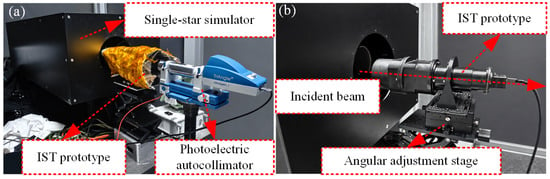
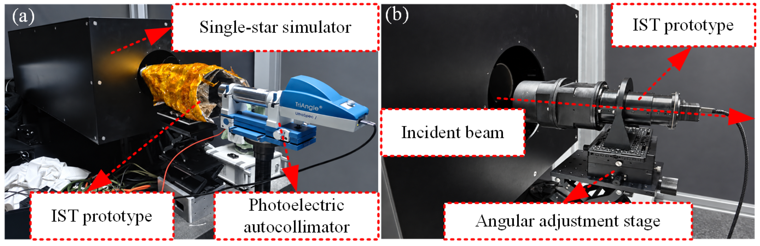
The static angular scanning experimental setup is shown in Figure 2. A single-star simulator was used to generate the incident beam, and the incident angle along the interferometric sensitive direction was adjusted by the angular adjustment stage. The detector outputs corresponding to the four measurement channels were recorded at each angular position and processed to obtain the normalized channel energy responses.

Figure 2. Static angular scanning experimental setup: (a) overall experimental setup; (b) IST prototype and angular adjustment configuration.

To quantitatively evaluate the agreement between the proposed model and the measured incident-angle-dependent responses, we compare single-star angular scanning data obtained with the prototype with the corresponding simulation results. The experimental scanning range is approximately 420.3 arcsec and consists of 85 angular positions. At each position, 10 consecutive frames are acquired, with an exposure time of 40 ms per frame. The experiment and simulation use the same grating period, grating separation, focusing lens focal length, detector array size, pixel size, and other system parameters listed in Table 1.

For each scanning position, we extract and average the integrated responses of the four target channels over the acquired frames. Because absolute quantities such as the source irradiance, actual system transmittance, and detector gain are difficult to match exactly between the experiment and simulation, the channel responses are normalized by the total energy of the four channels to focus the comparison on their relative energy distribution:

$${\tilde{I}}_k\left({\alpha }_i\right)={\displaystyle \frac{I_k\left({\alpha }_i\right)}{{\displaystyle {\sum }_{q=1}^4{I}_q\left({\alpha }_i\right)}}},\hspace{1em}k=1,2,3,4,$$

(56)

where $I_k\left({\alpha }_i\right)$ and ${\tilde{I}}_k\left({\alpha }_i\right)$ denote the integrated energy and normalized energy, respectively, of the kth channel at the ith angular position.

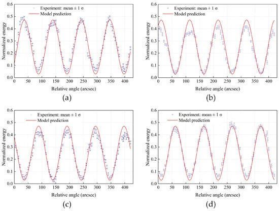
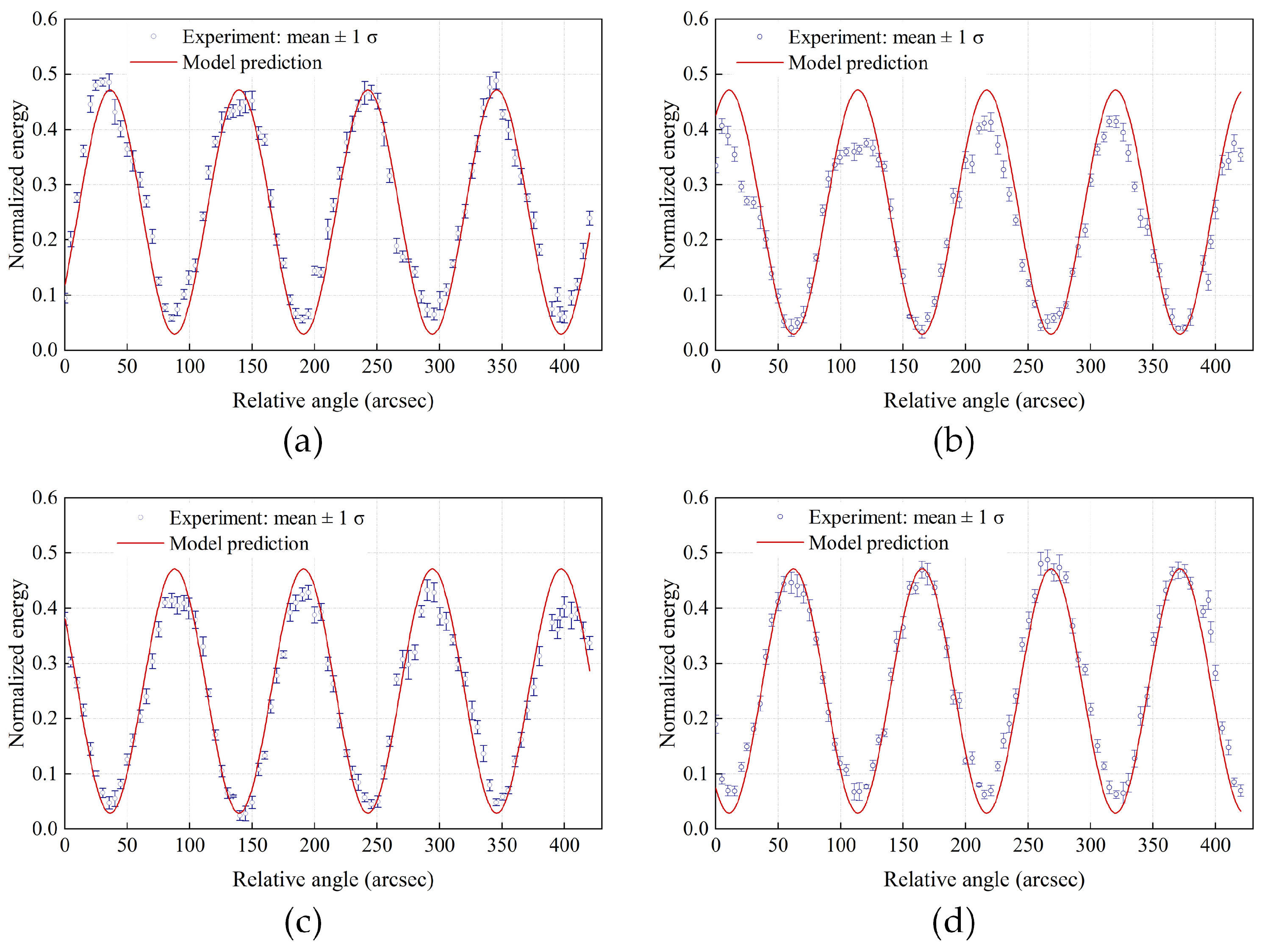
As shown in Figure 3, both the experimental and simulated results exhibit stable periodic energy modulation. The major peaks, valleys, and crossover positions of the four channels agree well, and the relative phase relationships between the complementary and quadrature channels are also consistent with the theoretical model. The correlation coefficients between the experimental and simulated responses of the four channels are 0.9814, 0.9775, 0.9817, and 0.9847, demonstrating that the proposed model captures the dominant incident-angle-dependent modulation characteristics of the four-channel response. The root-mean-square errors of the normalized channel energies range from 0.0359 to 0.0510. Although some discrepancies remain in the response amplitudes, the overall variation trends and the relative energy relationships among the channels agree well between the experiment and simulation.

Figure 3. Comparison of simulated and measured four-channel energy responses under static angular scanning: (a) Channel 1; (b) Channel 2; (c) Channel 3; (d) Channel 4.

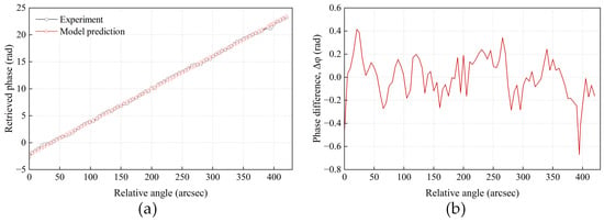
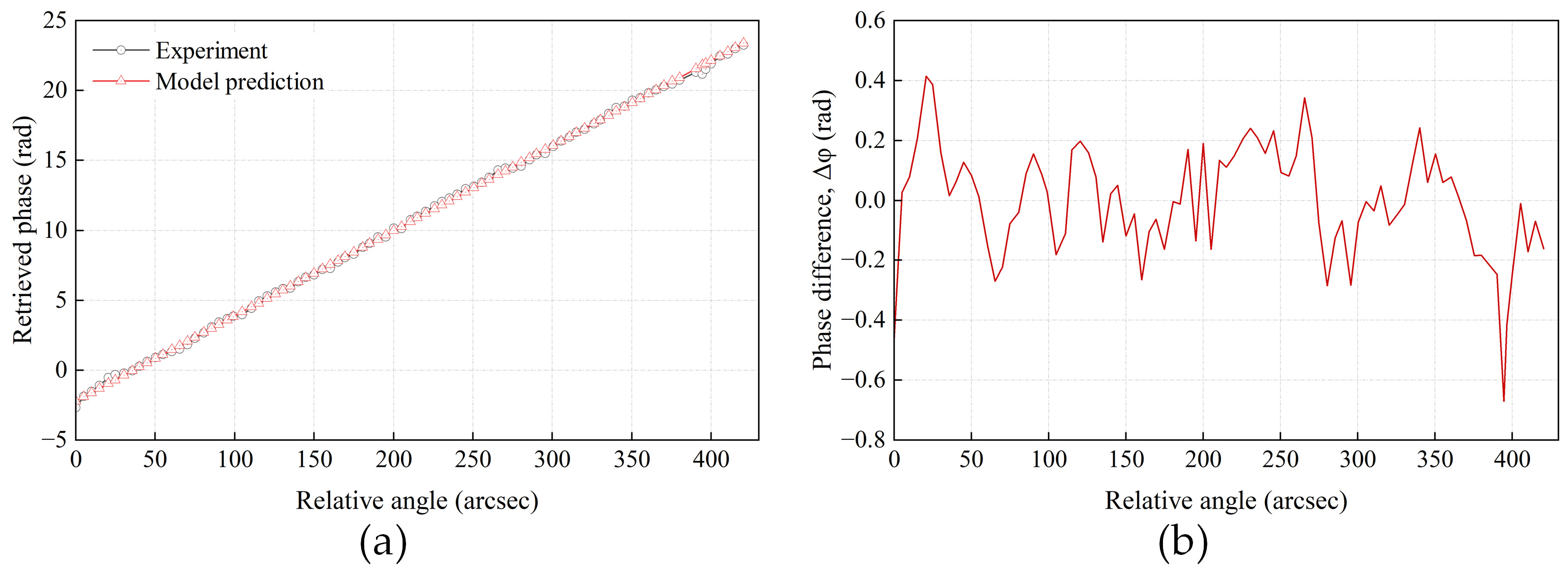
Because interference-phase evolution underlies the dynamic model, we further evaluated the phase responses retrieved from the experimental and simulated four-channel energies. Figure 4 compares these responses over approximately four interference periods. We retrieved experimental phases from the frame-averaged four-channel energies at each angular position. Both phase sequences were independently unwrapped along the scan, and their pointwise differences were calculated without subtracting a constant phase offset. The RMS phase discrepancy across the 85 angular positions was 0.1845 rad, with both responses exhibiting consistent angle-dependent variations. This comparison provides additional experimental support for the static phase response underlying the dynamic model.

Figure 4. Comparison of retrieved interferometric phase responses between simulation and experiment under static angular scanning: (a) retrieved phase responses; (b) phase difference.

The residual amplitude discrepancies may arise from grating fabrication tolerances, subaperture misalignment, detector flat-field nonuniformity, and PSF modeling approximations. These factors may contribute to the larger deviation in Channel 2, but the present comparison does not distinguish their individual contributions. No empirical channel-specific correction coefficients were introduced in the comparison. Normalization removes a common energy scale but does not eliminate channel-dependent mismatches, which may also affect dynamic phase retrieval.

5.3. Dynamic Interferometric Star-Image Simulation Results

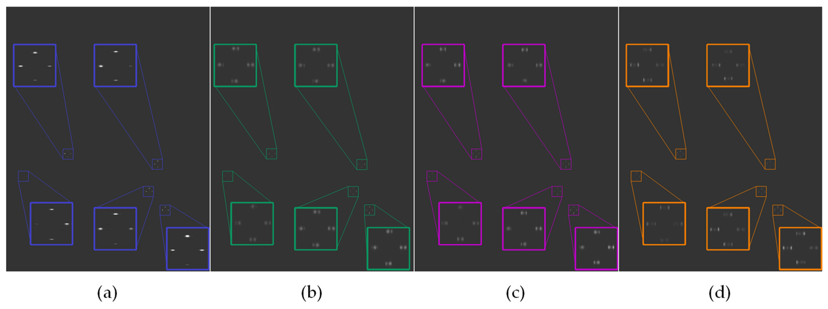
The four operating conditions defined in Section 5.1 were simulated using a 40 ms exposure. For these representative images, the constant-rate and periodic-jitter components were set to η = 1.5 and ξ = 1.5, respectively. Under the stated system parameters, these correspond to an angular rate of approximately 1.08°/s and a jitter amplitude of 59.25 arcsec.

Figure 5 shows the simulated dynamic interferometric star images under the four operating conditions, together with enlarged views of selected target regions. Under the static condition, the multichannel image points and diffraction structures associated with each star remain stable. Under dynamic conditions, both the multichannel image points and the diffraction structures exhibit nonuniform motion-induced smearing.

Figure 5. Simulated interferometric star images under different platform motion conditions: (a) static condition; (b) constant-rate angular motion; (c) periodic attitude jitter; (d) coupled constant-rate angular motion and periodic attitude jitter. The colorful squares indicate the corresponding star-spot regions used for image evaluation.

Platform motion changes both image positions and the phase-dependent energy distribution among channels. Dynamic images therefore cannot be represented by simply superposing translated copies of a fixed static image. Image smearing alone does not determine modulation retention, dynamic phase bias, or angular measurement reliability. These effects are quantified below using controlled single-star full-link simulations.

5.4. Performance Degradation Under Platform Motion

5.4.1. Constant-Rate Angular Motion

We use a single star with an apparent magnitude of 5 and an effective temperature of 5900 K as the target, with an exposure time of 40 ms. The normalized phase sweep η defined in Section 4 is varied from 0 to 2 in increments of 0.1, giving 21 motion conditions. For each condition, we run 1000 independent noisy simulations to evaluate the modulation retention factor and angular measurement error.

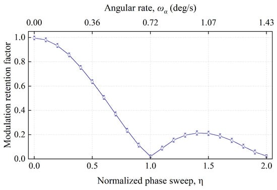
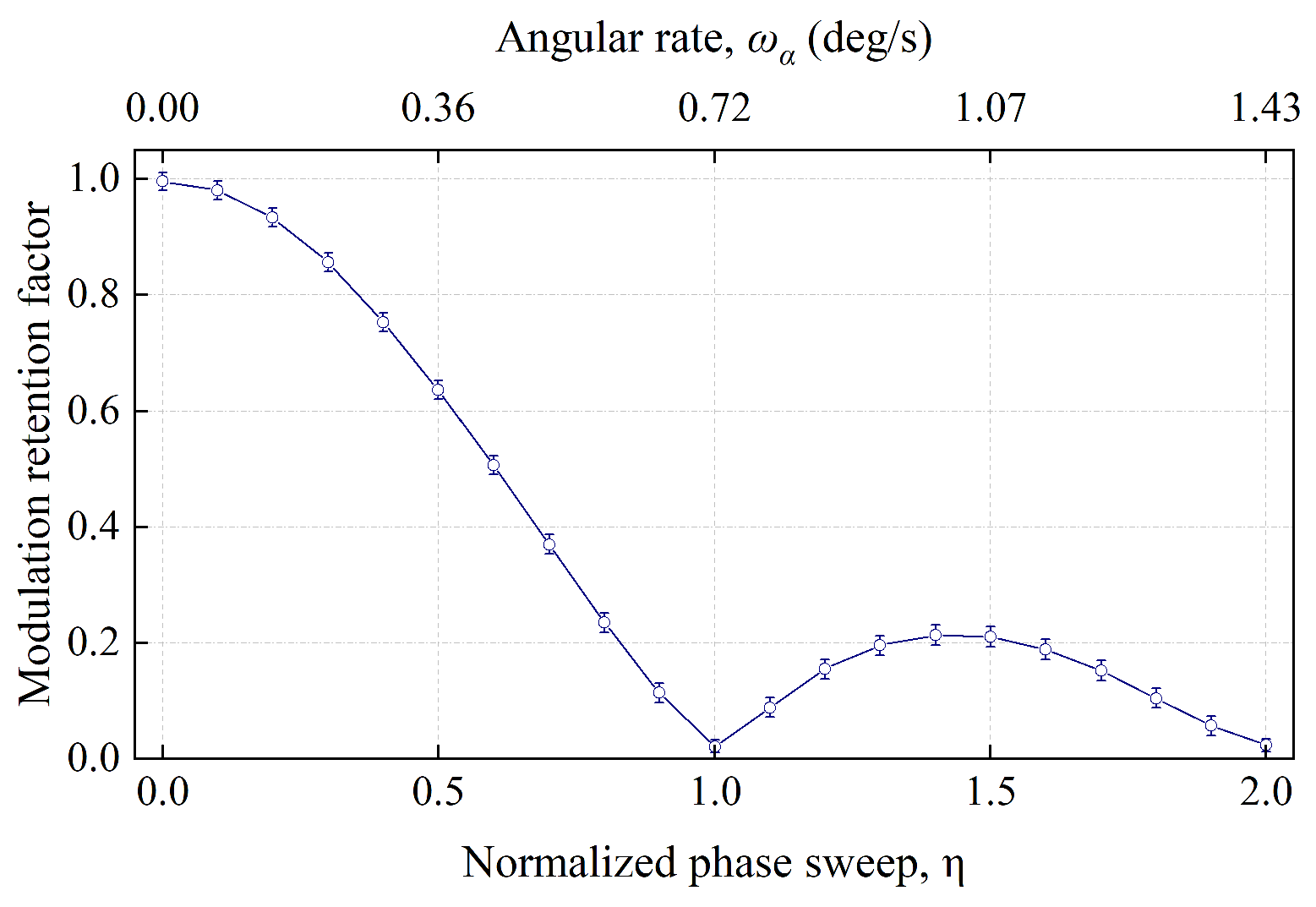
Figure 6 shows the modulation retention factor as a function of η. The full-link simulation results agree closely with the analytical sinc response. Within the first positive-response interval 0 < η < 1, the modulation retention factor decreases continuously as motion intensity increases. At η = 0.5, 0.8, and 0.9, the simulated values are approximately 0.64, 0.23, and 0.11, respectively. This agreement confirms that the sinc-type dynamic response remains dominant after including the complete imaging and detector processes in the full-link model.

Figure 6. Modulation retention factor under constant-rate angular motion with a 40 ms exposure. At each parameter point, 1000 noisy simulations were performed. Symbols and error bars indicate the mean and ±1 standard deviation, respectively; lines connect the means.

At η = 1, corresponding to an angular rate of approximately 0.72°/s, the sinc response reaches its first theoretical zero. Although the noisy simulation yields a residual modulation retention factor of approximately 0.02, this residual is mainly caused by the positive bias introduced when taking the magnitude of the noisy complex differential signal. It does not indicate retained coherent phase information and therefore does not represent an artificial lower bound of the usable modulation level.

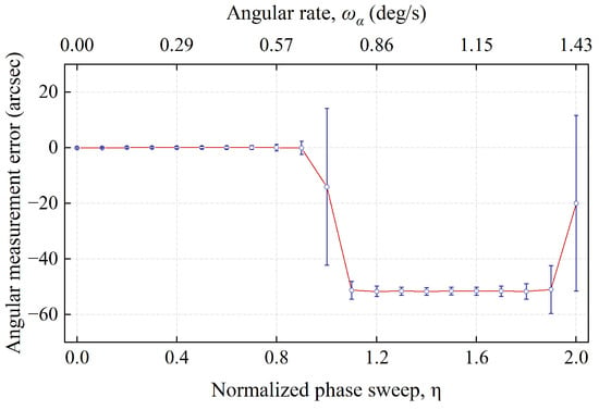
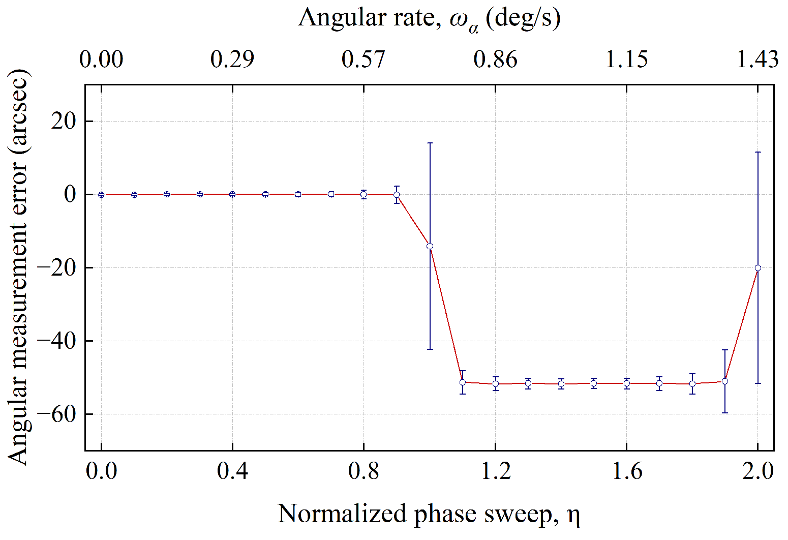
Figure 7 presents the mean and standard deviation of the angular measurement error. For 0 ≤ η < 1, the mean error remains close to zero, while the standard deviation increases as the modulation decreases. The standard deviation is approximately 0.269 arcsec under the static condition and increases to 0.413, 1.204, and 2.387 arcsec at η = 0.5, 0.8, and 0.9, respectively. As the first response zero is approached, the reduced complex differential amplitude leads to a rapid loss of phase observability and a pronounced increase in measurement dispersion.

Figure 7. Angular measurement error under constant-rate angular motion with a 40 ms exposure. At each parameter point, 1000 noisy simulations were performed. Symbols and error bars indicate the mean and ±1 standard deviation, respectively; lines connect the means.

For η > 1, the sinc response enters its first negative sidelobe. The reversal of the complex response introduces an approximately π phase shift. Because no motion state information or dynamic-response sign is used for phase-branch correction, the retrieved phase is still interpreted using the static phase-to-angle mapping and therefore falls onto an adjacent erroneous branch. Over 1 < η < 2, the mean angular measurement error remains approximately −51.5 arcsec, corresponding to about half an interferometric angular measurement period.

5.4.2. Periodic Attitude Jitter

A single star with an apparent magnitude of 5 and an effective temperature of 5900 K is used as the target, with an exposure time of 40 ms. The jitter frequency is first set to 25 Hz, so that each exposure spans exactly one jitter period. The normalized jitter-induced phase amplitude ξ is varied from 0 to 2, with additional sampling near the first response zero, resulting in 31 jitter conditions.

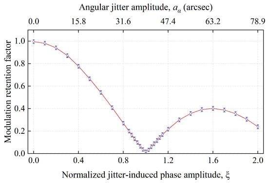
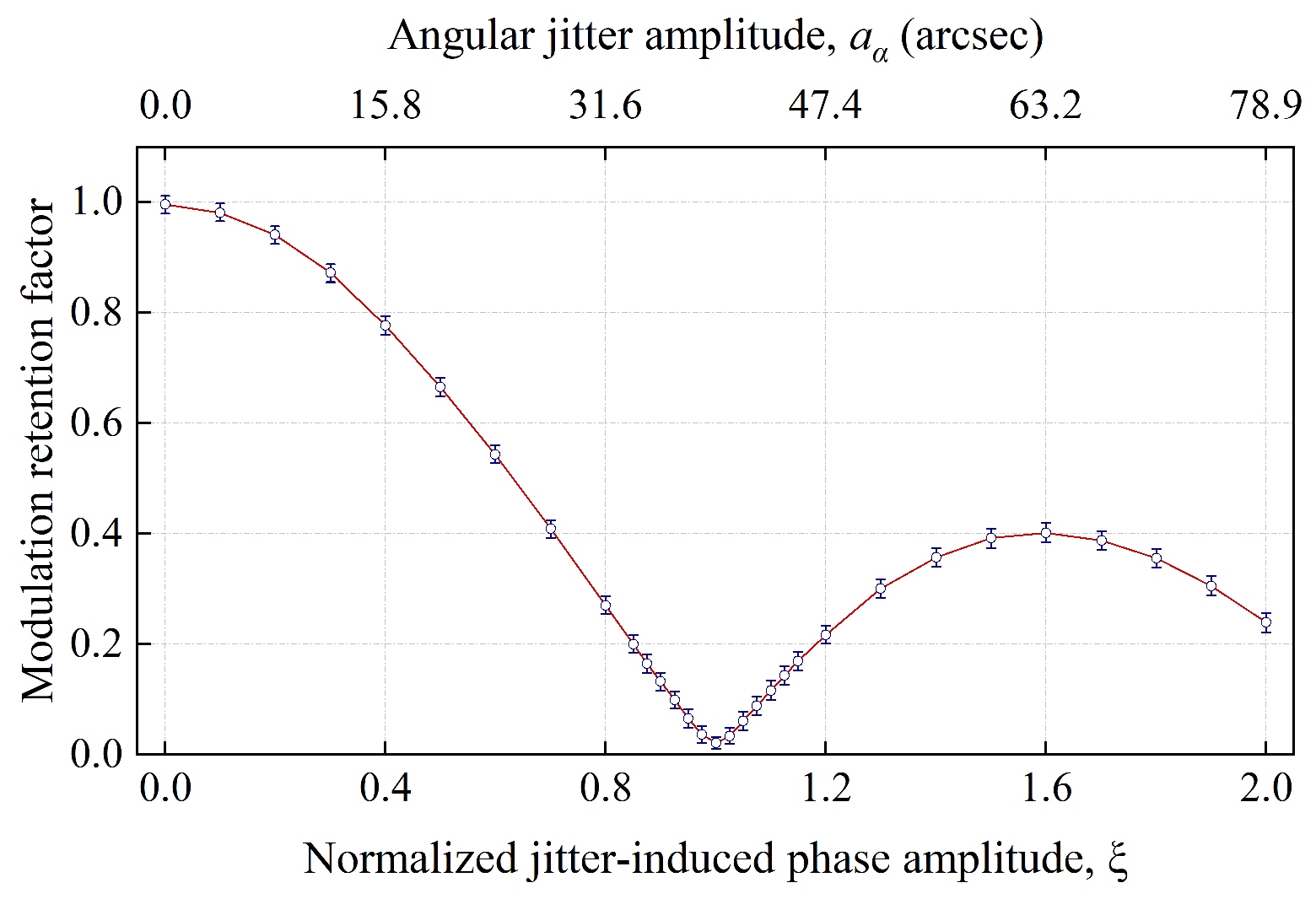
Figure 8 shows the modulation retention factor as a function of ξ. The full-link simulation results agree well with the analytical zeroth-order Bessel response. Within 0 < ξ < 1, the modulation decreases continuously and approaches zero at ξ = 1. The residual value of approximately 0.02 at the theoretical zero is caused mainly by the positive bias introduced when evaluating the magnitude of the noisy complex differential signal. This residual floor reflects the uncertainty of amplitude estimation near the zero-response region rather than a recoverable interferometric response. Beyond the first zero, the response enters the first negative lobe, with its magnitude reaching approximately 0.40 near ξ ≈ 1.6. These results confirm that the complete-period Bessel-type response remains valid in the full-link simulation.

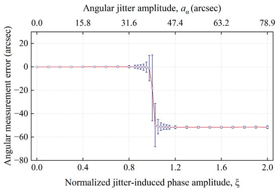
Figure 8. Modulation retention factor under periodic attitude jitter, with each 40 ms exposure spanning one complete jitter cycle. At each parameter point, 1000 noisy simulations were performed. Symbols and error bars indicate the mean and ±1 standard deviation, respectively; lines connect the means.

Figure 9 shows the corresponding angular measurement errors. The same three degradation regimes observed for the sinc response are reproduced here: random error amplification in the first positive-response interval, severe phase instability near the first zero, and phase-branch misidentification after the Bessel response changes sign. For ξ > 1, the reversal of the complex response introduces an approximately π phase shift, causing the mean angular measurement error to approach −51.5 arcsec when no dynamic phase-branch correction is applied.

Figure 9. Angular measurement error under periodic attitude jitter, with each 40 ms exposure spanning one complete jitter cycle. At each parameter point, 1000 noisy simulations were performed. Symbols and error bars indicate the mean and ±1 standard deviation, respectively; lines connect the means.

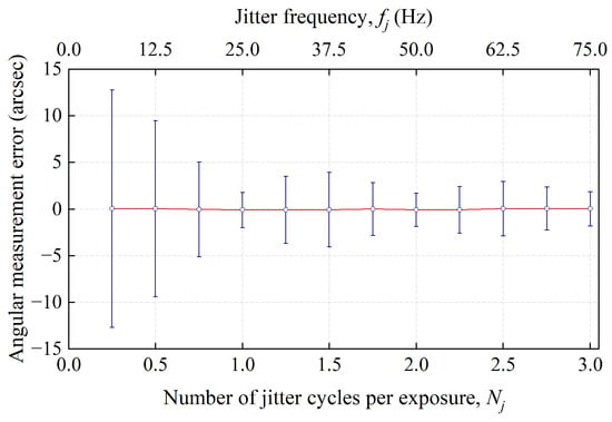
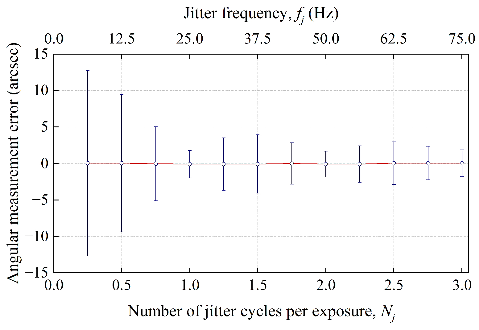
The above results correspond to an exposure containing exactly one jitter period, for which the dynamic response is independent of the jitter initial phase. In practice, however, the exposure time and jitter period are generally not exactly matched. To investigate this effect, ξ is fixed at 0.5, corresponding to an angular jitter amplitude of approximately 19.7 arcsec, while the number of jitter cycles per exposure, N_j = f_jT_e, is varied from 0.25 to 3.00 by changing the jitter frequency. For each N_j, 40 initial phases are uniformly sampled, with 25 independent noisy simulations performed for each phase.

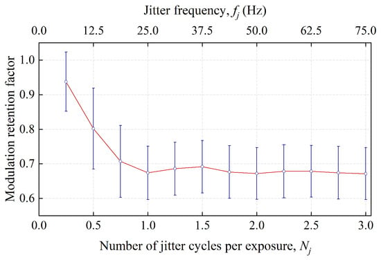
Figure 10 shows how the modulation retention factor varies with N_j. At N_j = 0.25, the exposure spans only one quarter of a jitter period, and the cancellation among complex phasors at different instants is relatively weak, resulting in a modulation retention factor of approximately 0.93. As the number of jitter cycles covered by the exposure increases, positive and negative angular deviations are more fully balanced within the exposure window. Consequently, the modulation retention factor generally decreases and gradually approaches the complete-period response of approximately 0.67, corresponding to the current jitter amplitude.

Figure 10. Modulation retention factor versus the number of jitter cycles per exposure at ξ = 0.5 and an exposure time of 40 ms. At each parameter point, 25 noisy simulations were performed for each of 40 uniformly sampled initial phases. Symbols show the pooled mean, and error bars indicate ±1 standard deviation across initial phases and noise realizations. Lines connect the means.

Figure 11 presents the angular measurement error under the same conditions. Although the overall mean error remains close to zero, this results from statistical cancellation of positive and negative phase shifts associated with different initial phases and does not imply negligible error for each phase. At N_j = 0.25 and 0.5, the error standard deviations are approximately 13 and 9 arcsec, respectively, despite the relatively high modulation retention factors.

Figure 11. Angular measurement error versus the number of jitter cycles per exposure at ξ = 0.5 and an exposure time of 40 ms. At each parameter point, 25 noisy simulations were performed for each of 40 uniformly sampled initial phases. Symbols show the pooled mean, and error bars indicate ±1 standard deviation across initial phases and noise realizations. Lines connect the means.

Since ξ = 0.5 remains within the first positive-response interval, no complex-response reversal occurs in this group of simulations. The results demonstrate that, under noninteger-period jitter, dynamic angular measurement performance depends not only on the jitter amplitude and frequency but also on the jitter initial phase. Therefore, both the magnitude and phase of the dynamic interference factor must be considered when evaluating measurement usability. In practical applications, if the dominant jitter frequency is known and sufficiently stable, exposure timing synchronization or integer-period exposure strategies can reduce this initial-phase sensitivity. However, for spacecraft disturbances with time-varying or multiple-frequency components, complete synchronization is difficult, and the proposed analysis provides a means to evaluate the resulting performance degradation.

5.4.3. Coupled Constant-Rate Angular Motion and Periodic Attitude Jitter

To validate the coupled-response model established in Section 4, a two-dimensional parameter sweep is performed over the normalized phase sweep η and normalized jitter-induced phase amplitude ξ. The target star has an apparent magnitude of 5 and an effective temperature of 5900 K. The exposure time is 40 ms, and the jitter frequency is fixed at 25 Hz. Both η and ξ are varied from 0 to 2 in increments of 0.1, resulting in 441 coupled-motion conditions. For each (η,ξ) condition, 20 jitter initial phases are uniformly sampled, with 50 independent noisy simulations performed for each phase, yielding 1000 measurement samples. The angular measurement uses only the four-channel exposure-integrated energies and the retrieved wrapped phase, without prior knowledge of the motion parameters, jitter initial phase, or dynamic-response sign and phase, and no phase-branch correction is applied. The maximum jitter amplitude is approximately 79 arcsec, and the total angular span during exposure remains below 1.8 × 10⁻³ rad. For reference angles within ±4.01°, this yields a conservative quadratic-to-linear phase-term ratio below 7 × 10⁻⁵, supporting the local linearization throughout the investigated parameter range.

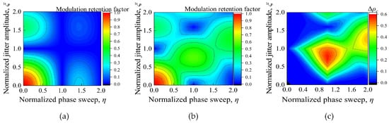
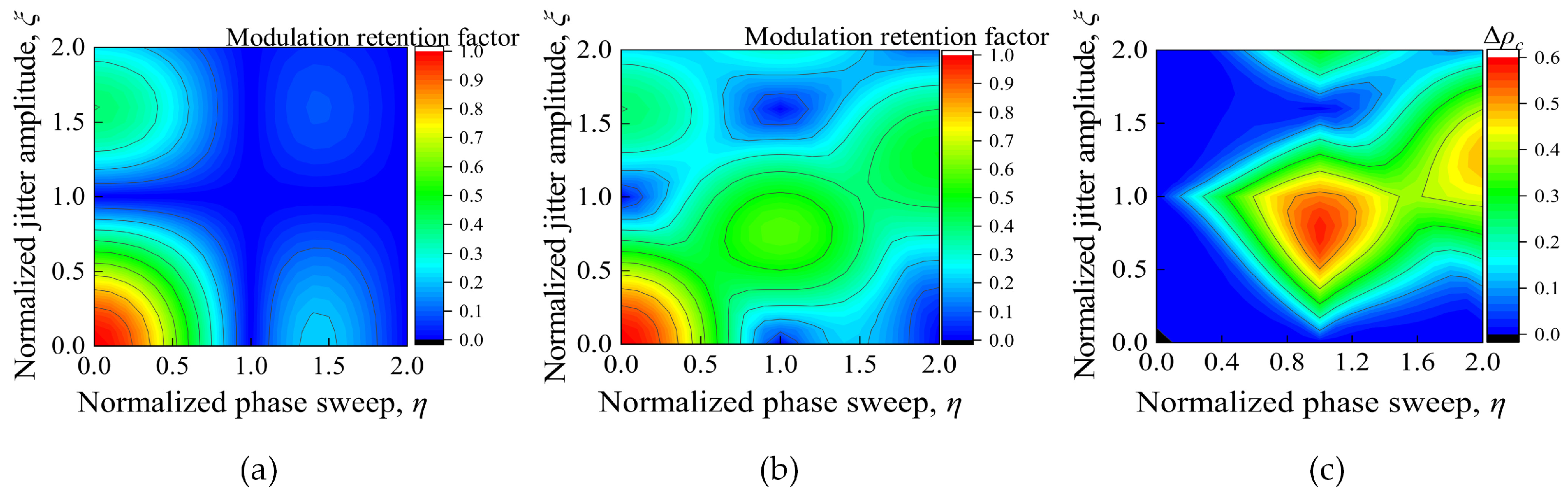
Figure 12 compares the modulation retention factors obtained from the independent sinc–Bessel product model and the full coupled model. The independent model produces vertical and horizontal low-response bands near η ≈ 1 and ξ ≈ 1, corresponding to the first zeros of the individual sinc and Bessel responses. In contrast, the full coupled response exhibits pronounced shifts, bending, and local filling of these low-response regions, demonstrating that the two motion components do not act as independent attenuation factors. The difference between the two models approaches zero along the individual motion boundaries η = 0 and ξ = 0, but increases substantially when both motion components are present, reaching approximately 0.58 near η ≈ 1 and ξ ≈ 0.8. Under the stated system parameters, this corresponds to an angular rate of approximately 0.72°/s and a jitter amplitude of approximately 31.6 arcsec.

Figure 12. Comparison between the independent sinc–Bessel product response and the full coupled response: (a) independent sinc–Bessel product response; (b) full coupled response; (c) difference in modulation retention factor.

This behavior agrees with the analytical model in Section 4. Constant-rate angular motion shifts the jitter-induced frequency components, which the finite-exposure sinc response then weights differently and coherently superimposes in the complex plane. Consequently, simultaneous motion cannot generally be represented by an independent sinc–Bessel product. Its applicability should be assessed using the modulation and phase error criteria in Section 4.2.3.

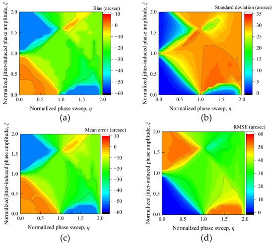
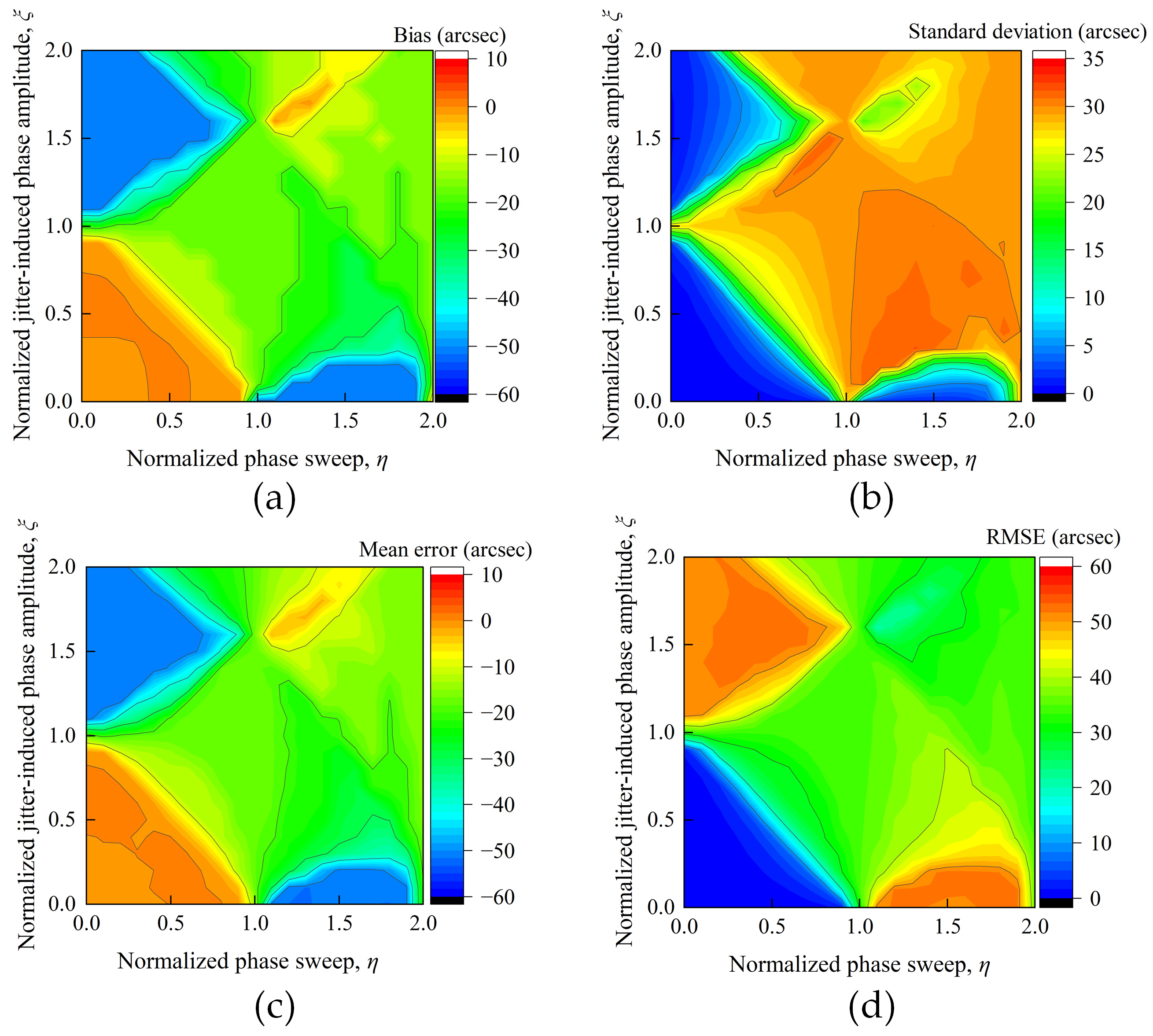
Figure 13 further evaluates the resulting angular measurement performance. The noise-free bias in Figure 13a and the Monte Carlo mean error in Figure 13c exhibit similar regional patterns. When both η and ξ are small, the response remains on a stable correct phase branch, and the angular bias is close to zero. As the motion intensity increases, changes in the dynamic phase and response direction lead to transitions between phase branches and systematic errors of several tens of arcseconds. Along the boundary ξ = 0, the results reduce to those of pure constant-rate angular motion: the bias remains close to zero for 0 ≤ η < 1 and approaches −51.5 arcsec after the first response zero.

Figure 13. Angular measurement performance under coupled constant-rate angular motion and periodic attitude jitter: (a) noise-free bias; (b) standard deviation of error; (c) mean error from Monte Carlo simulations; (d) RMSE.

The error standard deviation in Figure 13b is closely associated with the low-modulation regions of the full coupled response rather than varying monotonically with either motion parameter. This dispersion reflects both initial-phase dependence and detector noise, with low modulation increasing the sensitivity of phase retrieval to noise. The standard deviation can reach approximately 30 arcsec near low-response regions and rapidly varying coupled-response boundaries. By contrast, some stable erroneous-branch regions exhibit relatively small standard deviations despite large systematic biases. The RMSE in Figure 13d therefore reflects the combined effects of random-error amplification and phase-branch bias, and shows that the angular measurement failure regions cannot be inferred solely from the response zeros of the independent sinc–Bessel model.

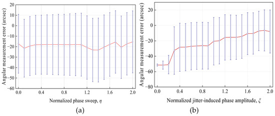
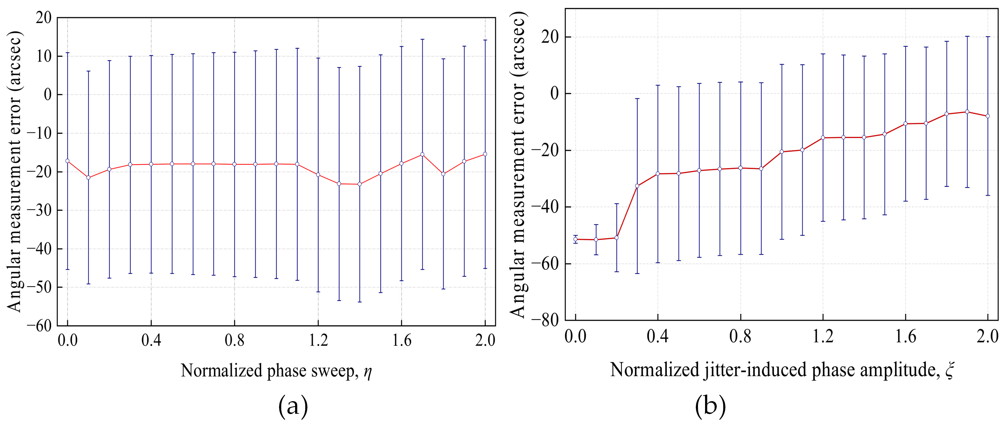
To illustrate the phase-branch evolution more clearly, Figure 14 presents two representative slices of the coupled-motion parameter space. At ξ = 1.0, the mean error remains approximately −15 to −24 arcsec over 0 ≤ η ≤ 2, without the distinct near-zero-error and −51.5 arcsec branches observed under pure constant-rate angular motion. The error dispersion also remains large, indicating strong phase-branch instability when periodic jitter is close to its individual response zero.

Figure 14. Angular measurement error along representative slices of the coupled-motion parameter space: (a) variation with normalized phase sweep η at ξ = 1.0; (b) variation with normalized jitter-induced phase amplitude ξ at η = 1.5. Each 40 ms exposure spans one complete jitter cycle. At each parameter point, 50 noisy simulations were performed for each of 20 uniformly sampled initial phases. Symbols show the pooled mean, and error bars indicate ±1 standard deviation across initial phases and noise realizations. Lines connect the means.

At η = 1.5, the condition ξ = 0 corresponds to the negative sidelobe of the pure constant-rate response, with a mean error of approximately −51.5 arcsec. As ξ increases, the mean error shifts toward zero and shows a pronounced transition near ξ ≈ 0.3, indicating that periodic attitude jitter modifies the magnitude and direction of the coupled-interference phasor and thereby changes the original erroneous phase branch.

For the stated integer-period exposure, the two models coincide on the single-motion axes within the local phase approximation. Near the weak-motion origin, the independent model also provides a first approximation to the phase-averaged modulation retention. However, near η ≈ 1 and ξ ≈ 0.8, it predicts nearly zero modulation, whereas the phase-averaged coupled retention is approximately 0.58. The full coupled response is therefore needed to assess operating limits where coupling displaces or fills the independent-response minima. For angular measurement assessment, the independent model must additionally satisfy both the modulation and phase criteria in Section 4.2.3.

6. Discussion

Previous dynamic star-tracker models relate image motion to star-spot spreading and localization errors. Yan et al. [8] derived a smeared-star energy distribution model and linked it to centroiding error and parameter selection. Yuan et al. [9] modeled rotational and angular vibration blur using trajectory, intensity, and PSF descriptors. These studies establish how motion affects image-based observables. The present results show that an IST additionally requires integration of its phase-dependent interference response during exposure. The resulting modulation cancellation and phase reversal cannot be characterized by star-spot displacement alone. The proposed framework therefore complements image motion modeling by accounting for the interferometric observable.

Our previous broadband IST model [18] described the static relationship between incident angle, multichannel energy distribution, and phase retrieval. The present work extends this relationship to time-varying incident angles through finite-exposure integration. Modulation retention and dynamic phase bias distinguish attenuation of the interference response from shifts in its effective phase. This distinction matters because, under the static inversion used here, modulation recovery in a negative sidelobe can coexist with a substantial angular bias. A retained modulation amplitude therefore does not, by itself, establish reliable angular measurement.

The coupled-motion results further reveal that separate single-motion responses cannot generally determine the combined response. The modulation retention difference of up to 0.58 within the investigated parameter range illustrates the potential error of the independent product approximation. Because both motion components act within the same phase integral, individual sinc or Bessel minima need not locate the minima of the coupled response. Following instrument-specific dynamic validation, the model could compare candidate exposure durations to balance motion-induced degradation against photon noise under the constraints in Section 4.3. If no exposure within the evaluated range meets these constraints, the model could assess whether reducing the angular rate or jitter would achieve the required accuracy. The full coupled response should be used when the independent approximation exceeds the allocated error tolerances.

The static angular scanning measurements support the multichannel response and phase–angle relationship underlying the dynamic model. Direct dynamic validation could use the IST prototype and a single-star simulator, with controlled angular motion along the interferometric sensing direction. A precision angular stage or tip–tilt mechanism synchronized with detector exposure could impose constant-rate motion, periodic jitter, or their combination. Static measurements under matched illumination and exposure conditions would provide the reference modulation amplitude. The exposure-integrated four-channel energies would then yield the modulation retention and phase for comparison with the model predictions. Recovered angles would be compared with calibrated reference angles, following the angular error definition used in the simulations. This focused experiment would test the predicted dynamic responses without reproducing the complete spacecraft disturbance environment.

7. Conclusions

We developed a full-link dynamic imaging model to evaluate angular measurement degradation in interferometric star trackers under finite-exposure platform motion. Static angular scanning experiments yielded four-channel response correlations above 0.97 and normalized-energy RMSE values of 0.0359–0.0510, supporting the modeled incident-angle-dependent response.

Under the local phase linearity condition, constant-rate angular motion and integer-period periodic jitter produce sinc-type and zeroth-order Bessel-type responses, respectively. For these two cases, modulation loss within the first positive-response interval primarily increases angular uncertainty. Under the static inversion used here, response sign reversals can cause phase-branch transitions and systematic angular bias. For noninteger-period jitter, angular errors also depend on the number of jitter cycles per exposure and the jitter initial phase.

Coupled constant-rate motion and single-frequency periodic jitter cannot generally be represented by an independent sinc–Bessel product. The maximum absolute difference in modulation retention between the coupled and independent models reaches approximately 0.58 within the investigated parameter range. The framework supports model-based assessment of angular motion operating limits, exposure selection, and platform stability requirements.

References

- Liebe, C.C. Accuracy Performance of Star Trackers—A Tutorial. IEEE Trans. Aerosp. Electron. Syst. 2002, 38, 587–599. [Google Scholar] [CrossRef] [Scilit]
- Jiang, J.; Zhang, G.J.; Wei, X.G.; Li, X. Rapid Star Tracking Algorithm for Star Sensor. IEEE Aerosp. Electron. Syst. Mag. 2009, 24, 23–33. [Google Scholar] [CrossRef] [Scilit]
- Ma, L.; Dai, D.; Ni, Y. How to Improve the Attitude Accuracy of the Star Sensor under Dynamic Conditions: A Review. Acta Astronaut. 2025, 233, 42–54. [Google Scholar] [CrossRef] [Scilit]
- Sun, T.; Xing, F.; You, Z.; Wang, X.; Li, B. Smearing Model and Restoration of Star Image under Conditions of Variable Angular Velocity and Long Exposure Time. Opt. Express 2014, 22, 6009. [Google Scholar] [CrossRef] [Scilit]
- Wu, X.J.; Wang, X.L. Multiple Blur of Star Image and the Restoration under Dynamic Conditions. Acta Astronaut. 2011, 68, 1903–1913. [Google Scholar] [CrossRef] [Scilit]
- Shen, J.; Zhang, G.J.; Wei, X.G. Simulation Analysis of Dynamic Working Performance for Star Trackers. J. Opt. Soc. Am. A 2010, 27, 2638. [Google Scholar] [CrossRef] [Scilit]
- Yang, H.; Jin, Y.; Hu, Y.; Zhang, D.; Yu, Y.; Liu, J.; Li, J.; Jiang, X.; Yu, X. Image Degradation Model for Dynamic Star Maps in Multiple Scenarios. Photonics 2022, 9, 673. [Google Scholar] [CrossRef] [Scilit]
- Yan, J.; Jiang, J.; Zhang, G. Dynamic Imaging Model and Parameter Optimization for a Star Tracker. Opt. Express 2016, 24, 5961. [Google Scholar] [CrossRef] [Scilit]
- Yuan, H.; Lu, K.; Liu, Q. Motion Modeling and Blurred Image Simulation of the Star Tracker Used for Deep-Space Missions. J. Opt. Soc. Am. B 2022, 39, 2934. [Google Scholar] [CrossRef] [Scilit]
- Tian, L.; Jiang, J.; Yang, J.; Ma, Y. Attitude Modeling of Star Trackers under Complex Vibration Conditions. Measurement 2024, 226, 114087. [Google Scholar] [CrossRef] [Scilit]
- Held, D.N. Interferometric Daylight Star Tracker. U.S. Patent 3,626,192, 7 December 1971. [Google Scholar]
- DeCou, A. Spacecraft Attitude Measurement Using Spatial Coherence of Laser or Star Light. IEEE Trans. Aerosp. Electron. Syst. 1971, AES-7, 288–298. [Google Scholar] [CrossRef] [Scilit]
- DeCou, A.B. Interferometric Star Tracking. Appl. Opt. 1974, 13, 414. [Google Scholar] [CrossRef] [Scilit]
- Hutchin, R.A. Interferometric Tracking Device. U.S. Patent 8 045 178 B2, 25 October 2011. [Google Scholar]
- Dong, L.; Wang, B. Research on the New Detection Method of Suppressing the Skylight Background Based on the Shearing Interference and the Phase Modulation. Opt. Express 2020, 28, 12518. [Google Scholar] [CrossRef] [Scilit]
- Zhang, S.F.; Jiang, S.; Dong, L.; Wang, J.L.; Wu, N.; Li, W.H. High accuracy interferometric star tracker based on diffraction grating. Chin. Opt. 2021, 14, 1368–1377. [Google Scholar] [CrossRef] [Scilit]
- Ruan, Y.X.; Dong, L. Influencing factors of angle measurement accuracy of an interferometer star tracker. Chin. Opt. 2023, 16, 1433–1441. [Google Scholar] [CrossRef] [Scilit]
- Yao, S.; Wang, H.Y.; Zheng, X.J.; Yan, Z.Q.; Liao, Z.; Zang, Y.Z. A Phase-Compensation-Based Method for Improving the Centroiding Accuracy of Interferometric Star Trackers. IEEE Trans. Instrum. Meas. 2026, 75, 4501212. [Google Scholar] [CrossRef] [Scilit]
- Dong, L.; Ruan, Y.X.; Wang, J.L.; Wang, B.; Li, H.Z.; Guo, P.; Wu, Y.H.; Jiang, S.; Zhang, S.F.; Wei, P.F. Progress in High Accurate Angle Measurement Technology of Long-Distance Target Based on Computational Interferometry. Laser Optoelectron. Prog. 2021, 58, 1811016. [Google Scholar] [CrossRef] [Scilit]
- U.S. Naval Observatory. USNO’s NISTEx-II Instrument Successfully Launched on May 4, 2019. 2019. Available online: https://www.cnmoc.usff.navy.mil/Portals/49/NISTEx%20Press%20Release_190513.pdf (accessed on 4 September 2026).
- Powell, R.L.; Stetson, K.A. Interferometric Vibration Analysis by Wavefront Reconstruction. J. Opt. Soc. Am. 1965, 55, 1593. [Google Scholar] [CrossRef] [Scilit]
- Wang, J. Evaluation Method for Noise-Induced Phase Error in Fringe Projection Profilometry. Appl. Opt. 2022, 61, 6167. [Google Scholar] [CrossRef] [Scilit]
Disclaimer/Publisher’s Note: The statements, opinions and data contained in all publications are solely those of the individual author(s) and contributor(s) and not of MDPI and/or the editor(s). MDPI and/or the editor(s) disclaim responsibility for any injury to people or property resulting from any ideas, methods, instructions or products referred to in the content. |
© 2026 by the authors. Licensee MDPI, Basel, Switzerland. This article is an open access article distributed under the terms and conditions of the Creative Commons Attribution (CC BY) license.