


Abstract
Generalizable 3D Gaussian Splatting enables efficient sparse-view novel view synthesis, but accurate Gaussian center estimation remains challenging. Epipolar attention and cost volume methods exhibit complementary limitations in non-Lambertian regions, appearance-ambiguous areas, and scenes with large perspective changes. These limitations lead to feature mismatches, depth estimation errors, and geometric distortions. To address these limitations, we propose GeoSplat, a feed-forward Generalizable 3D Gaussian Splatting framework with geometry-aware priors. Specifically, we introduce a geometry-aware cost volume that injects relative pose distance, view-dependent ray angle, and spatial validity masks into dense depth matching, enabling the network to jointly reason about photometric consistency, triangulation reliability, and visibility. Furthermore, we design a ray-guided iterative refinement module, in which full-resolution 3D ray direction and depth confidence priors jointly guide recurrent residual updates to progressively refine coarse depth predictions in a continuous space. Extensive experiments on RealEstate10K and ACID demonstrate that GeoSplat achieves competitive reconstruction quality with a compact parameter count, while presenting an accuracy efficiency trade-off.
1. Introduction
Single-scene 3D Gaussian Splatting (3DGS) has significantly advanced novel view synthesis due to its explicit scene representation and rasterization-friendly rendering pipeline. By representing a scene as a set of 3D Gaussian primitives, 3DGS enables high-quality rendering with remarkable efficiency [1]. However, conventional 3DGS still requires dense multi-view images and time-consuming per-scene optimization, which limits its applicability to unseen scenes and sparse-view scenarios. To address this limitation, recent Generalizable 3DGS (G-3DGS) methods employ feed-forward networks to directly predict 3D Gaussian parameters from sparse input views. Among these parameters, the 3D Gaussian means, i.e., the spatial centers of Gaussian primitives, are particularly critical because they determine the underlying scene geometry. Since Gaussian centers are usually obtained by estimating pixel-level depth and back-projecting pixels into 3D space, the quality of depth prediction directly affects the geometric consistency and rendering fidelity of the final novel views [2,3,4,5,6,7].
However, three key challenges remain in sparse-view G-3DGS. First, epipolar attention and plane sweep cost volumes exhibit complementary failures. pixelSplat [3] captures reliable correspondences but becomes unstable under view-dependent appearance changes, blurring Gaussian centers in non-Lambertian regions. MVSplat [4] better handles ambiguity and repetitive textures yet can favor inconsistent depths near sharp boundaries, occlusions, large perspective changes, and weak overlap areas. Second, conventional cost volumes rely mainly on appearance similarity and cannot determine whether correspondences are geometrically valid. Without camera baseline, ray intersection, and projection validity cues, the network may confuse mismatches with occlusions or invalid projections. Explicitly concatenating visual features and geometric metadata creates a large 5D tensor, while feature compression weakens matching discrimination. Third, even a reliable initial depth distribution remains constrained by discrete fronto-parallel hypotheses. Such sampling only coarsely approximates continuous slanted surfaces, causing staircase artifacts on angled walls, floors, and ceilings. These errors propagate through back-projection to Gaussian centers, motivating ray- and confidence-guided recurrent residual correction beyond the sampled depth planes.
To address these challenges, we propose GeoSplat, a memory-efficient feed-forward G-3DGS framework from sparse multi-view images with geometry-aware priors. An overview of the qualitative and efficiency advantages of GeoSplat is presented in Figure 1. The core idea is to explicitly inject geometric priors into the depth estimation process while preserving a compact memory footprint. Specifically, we introduce a geometry-aware cost volume that augments appearance-based matching with relative pose distance, view-dependent ray angle, and spatial validity masks. These priors allow the network to evaluate depth candidates according to baseline condition, ray intersection stability, and visibility, thereby disentangling appearance-induced mismatches from occlusions or invalid projections. As a result, GeoSplat preserves sharp structures in geometry-rich regions while improving robustness in appearance-ambiguous or non-Lambertian regions, repetitive textures, and weak overlap regions. However, a reliable initial depth distribution is still insufficient for accurate Gaussian mean localization because discrete fronto-parallel hypotheses cannot fully represent continuous slanted surfaces. We therefore introduce a ray-guided iterative refinement module inspired by PatchMatch Stereo [8]. Ray direction and confidence priors guide recurrent residual updates, propagate reliable geometry from confident regions to uncertain areas, and progressively correct coarse depth in continuous space. Overall, GeoSplat realizes Generalizable 3D Gaussian Splatting from sparse multi-view images through geometry-aware priors. It establishes a geometry-complementary Gaussian architecture in which memory-efficient matching provides initial geometry, while ray-guided iterative refinement corrects discretization errors in continuous space. This design improves Gaussian mean localization while preserving model compactness and inference efficiency.
Figure 1.
Qualitative and efficiency comparisons of GeoSplat. (a) Given sparse-view input images, GeoSplat produces more faithful novel views than PixelSplat and MVSplat, particularly in low-texture regions, weakly matched areas, and complex geometric structures. It preserves clearer boundaries and finer scene details while reducing blurring and structural distortions. (b) Comparison of reconstruction accuracy, inference time, and model size on RealEstate10K, where the horizontal axis denotes inference time, the vertical axis denotes PSNR, and the bubble size represents the number of parameters. GeoSplat achieves a favorable balance between reconstruction quality, inference efficiency, and model compactness.
The main contributions of our work are summarized as follows:
To address the complementary failure modes of existing sparse-view G-3DGS methods, we propose GeoSplat, a geometry-complementary feed-forward framework that coordinates geometry-aware matching and continuous depth refinement, improving Gaussian center estimation while maintaining a compact model size and efficient inference.
To resolve unreliable appearance-driven depth matching, we design a geometry-aware cost volume that reformulates depth hypothesis evaluation using relative pose, ray angle, and visibility cues, improving matching reliability in non-Lambertian regions, repetitive textures, occlusions, and weak overlap areas.
To alleviate discretization errors introduced by fronto-parallel inverse depth hypotheses, we propose a ray-guided iterative refinement module, in which ray direction and confidence priors guide recurrent residual depth updates in a continuous space, reducing staircase artifacts and improving Gaussian center localization.
Extensive experiments on RealEstate10K and ACID demonstrate that GeoSplat achieves competitive reconstruction quality while maintaining a compact parameter count and presenting an accuracy–efficiency trade-off relative to faster baselines.
2. Related Work
2.1. Novel View Synthesis
Novel view synthesis (NVS) aims to generate photorealistic images from unobserved viewpoints, requiring both accurate scene representation and efficient rendering. Neural Radiance Field (NeRF)-based methods have achieved remarkable progress by representing scenes as continuous radiance fields parameterized by multi-layer perceptrons. However, NeRF-based methods rely on dense volumetric sampling along camera rays, leading to high computational costs and limiting their applicability to real-time rendering [9].
Recently, 3D Gaussian Splatting (3DGS) has emerged as an efficient alternative for novel view synthesis [1]. Instead of using implicit volumetric fields, 3DGS explicitly represents a scene with a set of anisotropic 3D Gaussian primitives and renders images through differentiable rasterization. This explicit representation enables high-quality rendering with significantly improved efficiency [10]. Nevertheless, standard 3DGS still depends on dense multi-view inputs and requires time-consuming per-scene optimization, which restricts its ability to generalize to unseen scenes and sparse-view scenarios.
To overcome this limitation, recent works have explored feed-forward reconstruction frameworks that directly infer 3D scene representations from sparse input views [11,12,13,14]. Compared with per-scene optimization methods, these generalizable approaches can reconstruct novel scenes in a single forward pass, making them more suitable for efficient sparse-view novel view synthesis. However, under limited view observations, accurately estimating scene geometry remains challenging, especially when reliable cross-view correspondence is unavailable. This challenge has motivated the development of generalizable 3DGS methods that predict 3D Gaussian parameters directly from sparse-view images.
Building on this direction, GeoSplat introduces geometry-aware priors into feed-forward Gaussian reconstruction, enabling more reliable geometry estimation while achieving a favorable balance among reconstruction quality, model compactness, and inference efficiency.
2.2. Multi-View Stereo
Multi-view stereo (MVS) aims to reconstruct 3D scene geometry from multiple calibrated images by establishing cross-view correspondences and triangulating matched observations [15]. Recent learning-based MVS methods [16,17,18] typically construct plane sweep cost volumes to evaluate feature consistency across a set of depth hypotheses. The resulting cost volumes are then regularized to predict dense depth maps for individual views, which are subsequently fused into point clouds or surface representations.
Although these methods achieve strong reconstruction accuracy under sufficiently dense views and reliable correspondences, they often depend on dense depth supervision or multi-stage depth fusion pipelines. Their performance may also degrade in sparse-view settings, where limited overlap, repetitive textures, occlusions, and non-Lambertian appearance make correspondence estimation less reliable. In addition, independently predicting and fusing multiple depth maps introduces extra computational and processing overhead.
Classical multi-camera reconstruction pipelines may further improve reconstruction accuracy through a downstream geometric correction stage. Chen et al. [19] reconstructed point clouds from calibrated multi-camera observations and applied an adaptive point cloud correction algorithm after the initial reconstruction to reduce geometric errors. In contrast, GeoSplat performs geometry-aware depth matching and ray-guided iterative refinement before Gaussian prediction and does not employ a separate post-reconstruction point cloud correction module.
Geometry-aware reasoning has also been explored in 3D point cloud learning. Wang et al. [20] developed a geometry-aware point cloud framework to improve cutting-point localization under structural clutter and occlusion. Unlike such task-specific methods operating on reconstructed point clouds, GeoSplat estimates geometry directly from sparse calibrated images and incorporates pose, ray angle, and visibility priors into feed-forward 3D Gaussian reconstruction.
In contrast, GeoSplat adapts cost volume-based geometric reasoning to sparse-view feed-forward 3D Gaussian reconstruction. Rather than relying solely on feature similarity, it conditions depth hypothesis evaluation on relative pose, ray angle, and visibility information. The estimated geometry is directly converted into 3D Gaussian primitives without a separate point cloud fusion stage. Moreover, GeoSplat is trained using only RGB image supervision, avoiding the need for ground-truth depth maps and reducing the dependence on costly depth acquisition.
2.3. Sparse-View Generalizable 3DGS
Generalizable 3D Gaussian Splatting has become a promising direction for efficient sparse-view scene reconstruction and novel view synthesis. Unlike conventional 3DGS, which optimizes Gaussian primitives on a per-scene basis, generalizable 3DGS predicts Gaussian parameters through feed-forward networks, enabling fast reconstruction without per-scene optimization. Existing methods typically estimate pixel-level depth from sparse-view images and then unproject pixels into 3D space to obtain Gaussian centers. Therefore, reliable depth estimation and cross-view matching are central to the quality of the predicted 3D Gaussian representation [3,4,21,22,23,24].
Early feed-forward 3DGS methods directly predict 3D Gaussian primitives from image features. Splatter Image [25] predicts Gaussian parameters from a single image, enabling efficient object-level reconstruction. PixelSplat [3] extends this idea to sparse multi-view settings by using epipolar transformers to model depth distributions along epipolar lines. By leveraging epipolar geometry, PixelSplat can effectively capture cross-view correspondences when reliable matches are available. However, epipolar attention-based matching can become unreliable in appearance-ambiguous or non-Lambertian regions, such as shadows, highlights, glossy surfaces, and specular reflections and may further degrade under repetitive textures, occlusions, or limited view overlap.
To introduce stronger dense matching evidence, MVSplat [4] constructs a plane sweep cost volume and estimates depth through dense cross-view feature correlation. This cost volume formulation improves geometric accuracy and provides an explicit depth distribution for Gaussian center prediction. Subsequent methods further enhance sparse-view reconstruction by introducing depth confidence, deformable matching, monocular priors, graph-based aggregation, or iterative refinement [26,27]. For example, TranSplat [7] improves depth estimation by using depth-aware matching and depth refinement, while GraphSplat [2] adaptively combines cross-view and intra-view information to compensate for unreliable sparse correspondences. These methods demonstrate that robust depth estimation is crucial for improving generalizable 3DGS under sparse-view conditions.
LangSurf [28] embeds language features into surface-aligned Gaussians for open vocabulary 2D/3D scene understanding, whereas GeoSplat focuses on feed-forward novel view synthesis from sparse posed images without language supervision. CoSurfGS [29] addresses large-scale surface reconstruction through collaborative distributed learning, while GeoSplat estimates geometry from sparse input views using a single feed-forward model. Knowledge Distillation-Based Distributed Dynamic 3D Gaussian Splatting [30] uses distributed knowledge transfer and time-dependent Gaussian modeling for large-scale dynamic scenes, whereas GeoSplat improves static sparse-view reconstruction through geometry-aware cost volume matching and ray-guided refinement. CityGS-X [31] focuses on scalable and geometrically accurate large-scale scene reconstruction through a system-level architecture, whereas GeoSplat targets static sparse-view feed-forward reconstruction and does not evaluate distributed or large-scale settings.
Despite these advances, existing methods still face two limitations. First, most matching modules primarily rely on appearance or feature similarity, which may be unreliable in appearance-ambiguous or non-Lambertian regions, repetitive textures, occlusions, and weak overlap areas. Without explicitly considering multi-view geometry, the network may assign high confidence to visually similar but geometrically inconsistent depth candidates. Second, depth refinement is often performed by standard 2D convolutional networks, which lack explicit ray-level geometric priors and remain limited by discrete fronto-parallel inverse depth hypotheses. As a result, they may struggle to recover continuous slanted surfaces and fine geometric details.
GeoSplat addresses these limitations through a geometry-aware cost volume and ray-guided iterative refinement, improving Gaussian center localization in appearance-ambiguous, weak overlap, and slanted surface regions while maintaining a compact and efficient feed-forward architecture.
3. Method
Existing sparse-view G-3DGS methods mainly rely on either epipolar attention or appearance-driven cost volumes. PixelSplat captures correspondences along epipolar lines but becomes unreliable in appearance-ambiguous or non-Lambertian regions, leading to blurred Gaussian mean localization. MVSplat provides denser matching through plane sweep cost volumes, yet appearance-only similarity may favor geometrically inconsistent depths near sharp structures, occlusions, and weak overlap regions. Therefore, sparse-view G-3DGS should not rely solely on either paradigm. To address these limitations, GeoSplat explicitly introduces geometry-aware priors through a geometry-aware cost volume and ray-guided iterative refinement (RGIR), improving depth estimation and Gaussian center prediction while maintaining an efficient feed-forward architecture [3,4].
3.1. Geometry-Complementary Gaussian Architecture
In this section, we present the overall framework of GeoSplat, a feed-forward G-3DGS framework with geometry-aware priors. GeoSplat is specifically designed to improve Gaussian mean estimation under sparse-view conditions, where appearance ambiguity, unreliable correspondences, and discretized inverse depth hypotheses jointly limit geometric accuracy. Rather than estimating geometry solely from appearance-based correspondence, our framework conditions depth matching on explicit multi-view geometry and further corrects the resulting coarse depth in a continuous space.
As illustrated in Figure 2, GeoSplat takes sparse multi-view images and their camera parameters as input. A hybrid CNN–Transformer backbone first extracts multi-scale features and establishes cross-view feature interactions. These features are then processed by the proposed geometry-aware cost volume to obtain a coarse depth distribution, depth-aware features, and a confidence map. Subsequently, the coarse depth and high-resolution image features are passed to the ray-guided iterative refinement module, which progressively improves the depth surface before the refined depth is back-projected to determine pixel-wise Gaussian centers. The remaining Gaussian parameters are predicted from the refined depth-aware features and used for novel view rendering.
Figure 2.
Overview of GeoSplat. Sparse calibrated multi-view images are first processed by a hybrid CNN–Transformer backbone to extract local CNN features and cross-view Transformer features. The proposed geometry-complementary architecture then performs two coordinated stages. First, the geometry-aware cost volume (GACV) combines reference features, warped source features, relative pose distance, ray angle, and spatial validity priors to obtain coarse inverse depth and depth confidence. Its channel slicing avoids materializing depth-expanded and concatenated 5D features, keeping the original 128-channel reference for 2D cost volume refinement. Second, ray-guided iterative refinement integrates the initial geometry estimate, input images, high-resolution context features, and full-resolution ray directions. Recurrent residual updates progressively refine inverse depth in continuous space, reducing discretization and staircase artifacts and improving Gaussian-center localization. Finally, the refined depth and image features are converted into 3D Gaussian primitives for efficient novel-view rendering.
The framework consists of three key components. First, the hybrid CNN–Transformer backbone extracts local visual structures while modeling cross-view correspondence from sparse input images. Second, the geometry-aware cost volume reformulates depth hypothesis evaluation using relative pose distance, view-dependent ray angle, and spatial validity masks. These geometric priors allow the network to jointly assess feature similarity, triangulation stability, and projection validity, thereby suppressing appearance-induced mismatches and geometrically inconsistent depth candidates. To preserve high-dimensional visual features without constructing a massive concatenated 5D tensor, the geometry-aware fusion process is implemented through decomposed convolution.
Third, the ray-guided iterative refinement module addresses the discretization errors remaining in the coarse depth estimate. It treats full-resolution 3D ray directions as an explicit geometry-aware prior and uses depth confidence as reliability guidance. Through recurrent residual updates, the module progressively refines depth in a continuous space, improving the representation of slanted surfaces and the spatial localization of Gaussian centers.
Overall, GeoSplat establishes a problem-driven geometry-complementary Gaussian Architecture for generalizable 3D Gaussian Splatting from sparse multi-view images with geometry-aware priors. Its two coupled stages serve distinct but coordinated purposes: geometry-conditioned matching provides a reliable initial depth distribution, while ray-guided iterative refinement corrects the remaining depth discretization errors. Together with memory-efficient decomposed convolution, this design improves per-pixel depth estimation while maintaining a compact parameter count and an accuracy–efficiency trade-off relative to faster baselines.
3.2. Geometry-Aware Cost Volume
Existing sparse-view G-3DGS methods suffer from unreliable depth hypothesis evaluation because conventional matching is dominated by photometric or feature similarity and lacks explicit assessment of multi-view geometry. Without considering the relative camera configuration, triangulation stability, and projection validity, visually plausible but geometrically inconsistent depth candidates may receive high confidence, directly degrading depth estimation and Gaussian mean localization.
Epipolar attention-based methods can effectively exploit reliable correspondences in geometry-dominant regions. However, their matching becomes unstable under view-dependent appearance variations in appearance-ambiguous or non-Lambertian regions, such as shadows, highlights, glossy surfaces, and specular reflections. Plane sweep cost volumes provide denser matching evidence and are more robust to ambiguous appearance and repetitive textures. Nevertheless, appearance-driven cost volume construction may still favor geometrically inconsistent depth candidates around sharp structures, large perspective changes, occlusions, and weak overlap regions [3,4].
To address this problem, we design a geometry-aware cost volume that reformulates depth hypothesis evaluation using explicit geometric priors, including relative pose distance, view-dependent ray angle, and spatial validity masks. As illustrated in Figure 3, these priors enable the network to jointly assess photometric consistency, triangulation reliability, and visibility, thereby suppressing geometrically invalid matches while improving depth estimation in non-Lambertian regions, repetitive textures, occlusions, and geometry-dominant structures.
Figure 3.
The details of the geometry-aware cost volume module.
In feed-forward 3D Gaussian Splatting (3DGS) pipelines, such as MVSplat, the dense cost volume is typically constructed by evaluating the feature-level consistency between the reference feature map and the warped source feature map . For a specific depth candidate , the raw feature correlation is conventionally computed via the scaled dot-product:
3.2.1. Geometry-Aware Priors
To implement this design, we extract a set of explicit geometric priors to condition the correlation evaluation. First, let and denote their respective camera-to-world transformations. We compute the transformation from the reference camera coordinate system to the source camera coordinate system as follows:
where the rotation matrix and translation vector describe the relative rotation and translation from the reference view to the source view, respectively. The corresponding rotation measure and translation measure are defined as:
The combined pose distance is then computed as:
The rotation measure is dimensionless, whereas the translation measure retains the coordinate unit of the input camera poses. The two weighting coefficients and are fixed to 1 rather than learned, and no additional normalization is applied before combining the rotation and translation measures.
Second, for each reference pixel and depth hypothesis , we construct the corresponding 3D point and transform it into the source camera coordinate system. Let denote the normalized reference viewing ray, and let denote the normalized source viewing ray toward the hypothesized 3D point. The ray angle prior is represented by:
Thus, the ray angle prior is evaluated separately for every depth hypothesis and forms a candidate-indexed volume over the depth and spatial dimensions. The ray intersection angle indicates triangulation reliability: nearly parallel rays amplify image-space matching errors into large depth uncertainty, whereas well-conditioned intersections provide stronger depth evidence.
Third, projection validity is evaluated for each reference pixel and depth hypothesis . Let and denote the normalized source-image coordinates of the projected 3D point and let denote its source-view depth. The binary spatial validity mask is defined as:
The validity mask is not applied as a hard gate or used to assign a fixed cost. For out-of-bounds projections, source feature warping uses zero padding, while all invalid hypotheses retain as an explicit input to the learned fusion network. A projection that lies within the image bounds and has valid source-view depth is treated as spatially valid, retained in the cost volume, and processed through the learned aggregation of appearance and geometric cues.
By integrating these geometric priors, the proposed cost volume is transformed from a purely appearance-driven similarity tensor into a geometry-conditioned probabilistic representation. Specifically, the injected priors benefit the matching process in three aspects (). First, baseline awareness allows the network to adaptively balance triangulation strength and perspective distortion according to the relative pose distance. Second, geometric conditioning enables the model to evaluate the reliability of each depth hypothesis based on ray intersection stability. Third, projection validity conditioning distinguishes out-of-bounds or behind-camera warps from spatially valid samples, while occluded but spatially valid projections are handled implicitly by the learned fusion. These properties are particularly important in two-view sparse-input 3DGS pipelines, where the absence of multi-view redundancy makes photometric matching inherently fragile.
3.2.2. Geometry-Aware Feature Fusion via Decomposed Convolution
To integrate high-dimensional visual features and multi-dimensional geometric metadata, a straightforward implementation would explicitly concatenate the reference feature , the warped source feature , and the geometric metadata tensor into a massive 5D tensor:
where denotes the batch size, is the feature channel dimension produced by the feature extractor, denotes the number of inverse depth hypotheses, and represent spatial height and width, respectively. denotes broadcasting the reference feature along the depth dimension. Therefore, the concatenated tensor contains visual feature channels and 4 geometric metadata channels; denotes the fusion tensor constructed for each pixel–depth pair:
The pose distance is broadcasted along the depth and spatial dimensions where required. Consequently, invalid hypotheses enter the learned geometric branch through the zero-valued validity channel rather than being removed before aggregation.
However, directly applying 3D convolutions to such a concatenated tensor incurs prohibitive memory consumption, especially when dense inverse depth hypotheses and high-resolution feature maps are used.
Compressing visual features before cost volume construction reduces memory usage but weakens matching discriminability. We instead reformulate feature fusion as a decomposed convolution, preserving high-dimensional visual representations without explicitly materializing the concatenated 5D tensor.
To avoid explicitly materializing without reducing the feature channel dimension, we decompose the initial 3D convolution used to fuse the reference feature, warped source feature, and geometric metadata. This layer maps the input channels to output channels.
is obtained by removing the singleton depth dimension of . In our implementation, the layer uses unit stride, zero padding, and unit dilation. Because its depth-axis kernel size is 1, adjacent inverse depth hypotheses are not mixed, and the depth-invariant reference response computed by the 2D convolution is identical to that obtained from the corresponding 3D convolution at every depth index.
The reference and source branches use no bias, while the complete bias is added once through the geometric branch; all branch responses are summed before BatchNorm3D and ReLU. Therefore, the decomposition is exactly equivalent to the implemented first convolution, while avoiding materialization of the tensor. Under identical training settings with a batch size of 1 and 128 inverse depth hypotheses, the naïve 5D concatenation, a 32-channel feature compression (reduced from 128-channel feature), and the proposed decomposed implementation require 6.204 GB, 5.082 GB, and 5.204 GB of peak allocated GPU memory, respectively. Although feature compression attains the lowest memory usage, it reduces the matching feature dimensionality from 128 to 32 and therefore changes the matching representation. In contrast, the proposed formulation retains all 128 feature channels and reduces peak memory by 16.1% relative to naïve concatenation without changing the function of the first fusion convolution.
By computing the three branch responses independently and accumulating them in place, GACV preserves the backbone’s high-dimensional features with a compact memory footprint. Unlike feature compression approaches, it improves memory efficiency by reformulating the fusion computation rather than reducing feature dimensionality.
In summary, GACV conditions appearance-based depth hypothesis evaluation on pose, ray angle, and projection validity priors, while decomposed convolution preserves high-dimensional features with low memory overhead. It provides a reliable initial depth distribution, but discrete fronto-parallel hypotheses still limit the modeling of continuous slanted surfaces. The next section introduces the ray-guided iterative refinement module to correct these residual discretization errors and improves Gaussian center localization.
3.3. Ray-Guided Iterative Refinement
After constructing the geometry-aware cost volume, we obtain an initial coarse inverse depth map through soft-argmin regression over discretized inverse depth hypotheses. Although the geometry-aware priors introduced in the previous section substantially improve the reliability of depth probability estimation, the resulting coarse depth representation is still constrained by a finite set of fronto-parallel planes. This discretization is insufficient for accurately modeling continuous slanted surfaces, such as angled walls, floors, ceilings, and other planar structures observed under oblique viewpoints. Consequently, the coarse inverse depth map may exhibit staircase-like artifacts, which further lead to inaccurate Gaussian centers after depth back-projection.
Classical PatchMatch Stereo (PMS) [32] addresses this issue by explicitly maintaining slanted plane hypotheses, spatially propagating reliable candidates, and refining local depth estimates through iterative perturbation. However, directly adopting PMS in feed-forward 3DGS is impractical: per-pixel plane parameterization and random neighborhood sampling disrupt the regular dense-tensor computation pattern on GPUs and introduce additional memory and computational overhead. To retain the geometric advantages of PMS while preserving the efficiency of a convolutional framework, we introduce a ray-guided iterative refinement module. As illustrated in Figure 4, instead of explicitly searching over slanted plane parameters, our module conditions a lightweight recurrent U-Net on ray direction and confidence priors, enabling it to predict iterative residual depth corrections in a continuous and fully differentiable manner.
Figure 4.
The details of ray-guided iterative refinement.
3.3.1. Implicit Slanted Surface Fitting
Traditional PMS explicitly represents a local surface by solving a plane equation for each pixel. In contrast, we implicitly encode local slanted geometry through full-resolution 3D viewing-ray directions. For a homogeneous pixel coordinate in the reference view, the normalized camera ray is computed as
where denotes the camera intrinsic matrix. This produces a dense ray direction map
Unlike a standard 2D refinement network that takes only image features and coarse depth values as input, our ray-guided refinement network additionally receives explicit pixel-wise 3D directional priors. These priors describe how neighboring pixels correspond to different 3D rays in camera space. When combined with the coarse inverse depth map, the ray direction prior allows convolutional kernels to perceive the continuous angular variation of the local viewing geometry. As a result, the network can implicitly infer whether adjacent pixels are likely to lie on a continuous slanted surface, rather than restricting them to discrete fronto-parallel depth planes. This design eliminates the need for explicit plane parameter search while retaining the ability to refine depth along continuous 3D surfaces.
3.3.2. Confidence-Guided Implicit Propagation
In classical PMS, reliable inverse depth hypotheses are propagated from confident pixels to neighboring uncertain pixels. We emulate this propagation mechanism by extracting a confidence prior from the coarse probability volume. Given the probability volume
where is the number of inverse depth hypotheses, we compute the maximum probability at each pixel as
The confidence map indicates the certainty of the coarse depth estimate. Peaked depth distributions yield high confidence, whereas diffuse distributions produce low confidence, often in low-texture, occluded, reflective, or weak overlap regions.
We feed this confidence map into the refinement network as an explicit reliability prior. Within the multi-scale receptive field of the U-Net, acts as a soft guidance signal: high-confidence regions serve as geometric anchors, while low-confidence regions are corrected by adaptively aggregating contextual information from nearby reliable areas. In this way, the refinement network implicitly propagates stable geometric information without requiring hand-crafted neighborhood sampling or explicit hypothesis replacement.
3.3.3. Recurrent Residual Update
A single-pass refinement network may still be insufficient for correcting large local geometric deviations caused by discretized hypotheses or ambiguous matching. To retain end-to-end differentiability, we formulate the refinement process as unrolled recurrent residual updates in the inverse depth domain [33,34,35].
Let denote coarse inverse depth map obtained from the geometry-aware cost volume. At each refinement iteration , we construct the input tensor by concatenating the reference image , the upsampled projected feature , the previous inverse depth estimate , the confidence map , and the full-resolution ray direction map :
A lightweight refinement U-Net predicts a continuous inverse depth residual:
The inverse depth estimate is updated recurrently as
Before Gaussian prediction, the final inverse depth estimate is bounded by the view-specific inverse depth range and converted to camera-axis depth:
We use (T = 2) refinement iterations in all main experiments. The parameters of () and the Gaussian prediction heads are shared across iterations; during training, the rendered output from every iteration is supervised using , where (), while only the final estimate is used at inference.
Thus, ray-guided iterative refinement refines inverse depth in continuous space. Finally, the refined depth is back-projected into 3D space to determine the Gaussian means. Since each refinement step is guided by ray direction and confidence priors and progressively updates the depth through recurrent residual correction, the resulting Gaussian centers are more accurately localized on slanted surfaces, weakly textured regions, and geometrically complex structures. The entire module remains fully convolutional and end-to-end differentiable, introducing minimal computational overhead while effectively alleviating the discretization bottleneck of the initial cost volume depth estimation.
3.4. Gaussian Prediction
In this section, we leverage the refined depth and depth-aware features to predict the parameters of a set of 3D Gaussian primitives
that represent the scene. Following previous generalizable 3DGS methods, we predict one Gaussian primitive for each pixel from input views, thus [3,4].
3.4.1. Gaussian Center
We utilize the final refined depth to directly unproject each pixel into 3D space using the corresponding camera parameters. The resulting 3D points are selected as the centers of the 3D Gaussians.
3.4.2. Opacity
For each pixel, the opacity is closely related to the reliability of the predicted depth, since an accurate depth prediction indicates that the corresponding point lies on the scene surface. Therefore, we predict opacity using an MLP layer with the refined depth-aware feature as input.
3.4.3. Covariance and Color
Similar to 3D Gaussian Splatting and recent generalizable 3DGS methods [1,3,4], we predict spherical harmonic coefficients to represent the color . For the covariance matrix , we predict a scaling matrix and a rotation matrix and formulate it as
All Gaussian parameters are predicted by lightweight MLP layers.
In summary, GeoSplat realizes Generalizable 3D Gaussian Splatting from sparse multi-view images with geometry-aware priors through a coordinated matching-and-refinement pipeline. The geometry-aware cost volume provides reliable and memory-efficient initial depth estimation, while ray-guided iterative refinement corrects the remaining discretization errors in a continuous space. Together, these designs improve Gaussian center localization while maintaining a compact parameter count and an accuracy–efficiency trade-off relative to faster baselines.
4. Experiments
4.1. Experimental Setup
Datasets. We evaluate GeoSplat on two large-scale datasets, ACID [36] and RealEstate10K [37]. RealEstate10K consists of 67,477 training scenes and 6474 testing scenes, which are extracted from home walk-through videos collected from YouTube. The ACID dataset contains 11,075 training scenes and 1972 testing scenes, mainly focusing on aerial landscapes with wide-baseline viewpoints. Both datasets provide camera poses, making them suitable for evaluating sparse-view novel view synthesis. Following PixelSplat, we train GeoSplat using 2 input views per scene and test it on 3 novel target views. To further assess the cross-dataset generalization ability of GeoSplat, we additionally evaluate the model on 16 validation scenes from the object-centric DTU dataset [38], rendering 4 novel views for each scene.
Metrics and Implementation Details. We evaluate the quality of the synthesized RGB images using three widely adopted metrics: pixel-level PSNR, patch-level SSIM [39], and feature-level LPIPS [40]. All images are first rescaled while preserving their aspect ratios and then center-cropped to (256 256) pixels, with the camera intrinsics adjusted accordingly. GeoSplat adopts the same backbone configuration as MVSplat [4]. Specifically, a shallow ResNet-like CNN containing six residual blocks is followed by six stacked multi-view Transformer blocks, each consisting of one self-attention layer and one cross-attention layer. The backbone is initialized using the publicly available UniMatch pretrained weights and produces 128-channel features at one-quarter of the input resolution. Thus, for (256 256) inputs, the backbone features and the geometry-aware cost volume are constructed and initially refined at a resolution of (64 64). We uniformly sample (D = 128) inverse depth hypotheses in the inverse depth domain between the near and far depth planes. The depth range is set to ([1,100]) for RealEstate10K and ACID, while ([2.125,4.525]) is used for DTU. The coarse inverse depth and confidence maps are subsequently upsampled to the full (256 256) resolution, after which ray-guided iterative refinement performs 2 recurrent residual update iterations. We use a fixed global PyTorch seed of 111123 and DataLoader seeds of 1234, 2345, and 3456 for training, testing, and validation, respectively, with rank-dependent offsets for distributed training. The same dataset splits, evaluation indices, sampling protocol, and seed settings are used for all ablation variants. We follow the same data augmentation and context/target sampling strategy as MVSplat.
Our model is implemented in PyTorch and trained on four NVIDIA GeForce RTX 4090 GPUs with a per-GPU batch size of 4, corresponding to an effective batch size of 16. Training is conducted for 300,000 iterations using the Adam optimizer [41] with an initial learning rate of (), a 2000-step linear warm-up, cosine learning-rate decay, and a gradient clipping threshold of 0.5. Training is supervised using ground-truth RGB images, and the objective combines MSE and LPIPS losses with respective weights of 1 and 0.05.
4.2. Comparison with State-of-the-Art Methods
We compare GeoSplat with representative state-of-the-art methods for sparse-view novel view synthesis and Generalizable 3D Gaussian Splatting. The comparison includes NeRF-based methods such as pixelNeRF [42], GPNR [43], AttnRend [44], and MuRF [45], as well as recent generalizable 3DGS methods including PixelSplat [3], MVSplat [4], eFreeSplat [6], and TranSplat [7]. PixelSplat and MVSplat serve as strong baselines, representing epipolar attention-based and cost volume-based generalizable 3DGS pipelines, respectively.
Following the evaluation protocol used in prior work, we report quantitative performance on RealEstate10K and ACID by rendering three novel target views given two reference input views and averaging the results across all testing scenes. We exclude DepthSplat [27] (RealEstate10K:27.47 PSNR, 0.889 SSIM, and 0.114 LPIPS) and IDESplat [5] (RealEstate10K:27.80 PSNR, 0.893 SSIM, and 0.108 LPIPS) from the main comparison because they rely on joint training with external depth estimation datasets (both DepthSplat and IDESplat employ a pre-trained Depth Anything V2 backbone and UniMatch weights that differ from the UniMatch initialization used by MVSplat).
GeoSplat achieves competitive performance against existing baselines on RealEstate10K and ACID, with the quantitative results reported in Table 1. Qualitative comparisons in Figure 5 and Figure 6 reveal that baseline methods struggle to consistently reconstruct scenes where non-Lambertian regions and geometry-dominant structures coexist. In contrast, GeoSplat reconstructs fine details with more coherent geometric structures. In the second row of Figure 6, where reflective water surfaces and distinct geometric structures such as a lighthouse appear simultaneously, GeoSplat maintains structural integrity and produces smoother background transitions, whereas baseline methods tend to exhibit misalignment and distortion.
Table 1.
Quantitative comparisons with SOTA methods. We evaluate performance on RealEstate10K and ACID by rendering three novel views from two reference viewpoints and averaging the results across all testing scenes. The trainable parameter counts are 11.956 M for MVSplat and 12.024 M for GeoSplat. Inference time includes scene encoding and rendering. GeoSplat achieves competitive reconstruction quality with a compact parameter budget, while presenting an accuracy–efficiency trade-off relative to faster baselines. (Bold figures indicate the best, underlined figures indicate the second best).
Figure 5.
Qualitative comparisons with state-of-the-art methods on RealEstate10K. GeoSplat produces more faithful novel views across indoor and outdoor scenes, especially in regions with weak texture, view-dependent appearance variations, occlusions, and complex geometric structures.
Figure 6.
Qualitative comparisons with state-of-the-art methods on ACID.
For a controlled efficiency comparison, the inference times in Table 1 are reported only for PixelSplat, MVSplat, TranSplat, and GeoSplat. All four methods are evaluated under an identical inference protocol: an input resolution of 256 × 256, two context views, three target views, a batch size of one, an NVIDIA GeForce RTX 4090 GPU, CUDA 11.8, and PyTorch 2.1.2. For each scene, the reported latency consists of one scene encoder forward pass plus the average rendering latency per target view. The first five test samples are discarded as warm-up. Each measurement is repeated three times, and Table 1 reports the mean and standard deviation across the three runs. Under this controlled protocol, GeoSplat achieves a competitive runtime: it is faster than PixelSplat while incurring higher latency than MVSplat.
To further analyze the geometric reconstruction quality, we visualize the intermediate depth maps predicted by different methods in Figure 7. The results show that baseline methods often produce noisy, distorted, or over-smoothed depth maps in challenging regions, such as reflective water surfaces, weak-texture areas, and indoor scenes with strong depth discontinuities. These unreliable depth predictions further lead to blurred novel views and geometric misalignment. Such errors are particularly evident around thin structures and occlusion boundaries, where inaccurate depth causes local Gaussian centers to drift, weakening foreground sharpness, background continuity, and cross-view consistency. These artifacts also disrupt local surface continuity and reduce the stability of depth transitions across neighboring pixels.
Figure 7.
Comparisons of synthesized views and intermediate depth maps.
In contrast, GeoSplat generates smoother and more structurally consistent depth maps, with clearer object boundaries and more stable planar regions. This demonstrates that the proposed geometry-aware cost volume provides more reliable initial depth distributions, while the ray-guided iterative refinement module further improves depth accuracy in a continuous space. As a result, GeoSplat achieves higher-quality geometric reconstruction and more faithful novel view synthesis.
4.3. Cross-Dataset Generalization
Following MVSplat [4], we directly evaluate models trained on RealEstate10K on the unseen DTU and ACID datasets without fine-tuning. As shown in Table 2 and Figure 8, GeoSplat achieves the best overall performance among the compared methods on ACID, yet its performance degrades significantly on DTU, where it falls behind most baselines. These results suggest that GeoSplat has a reasonable capacity to generalize to outdoor aerial scenes with wide-baseline viewpoints and large-scale geometric layouts.
Table 2.
Cross-dataset generalization. Zero-shot tests on the DTU and ACID using models trained on RealEstate10K (bold figures indicate the best, underlined figures indicate the second best).
Figure 8.
Cross-dataset generalization. Models trained on RealEstate10K are directly used to render scenes from the target datasets DTU (first row) and ACID (last row).
However, GeoSplat performs less favorably on DTU than MVSplat and TranSplat. Compared with the outdoor aerial scenes in ACID, DTU comprises close-range, object-centric scenes with small foreground objects and markedly different depth scales and viewpoint distributions. This distribution shift may make the camera configuration and ray geometry priors used by GeoSplat less well aligned with the depth matching requirements of DTU, which may contribute to blurred or incomplete object reconstruction. In particular, the translation component of our pose prior is represented by the raw relative translation magnitude without explicit scene scale normalization. This design is therefore not strictly scale-invariant across datasets; however, the present results do not establish it as the sole cause of the DTU performance gap. The direct depth results in Table 3 indicate that GeoSplat does not exhibit a large systematic bias in the directly predicted context-view depth maps.
Table 3.
Direct depth accuracy on DTU. Lower values are better.
GeoSplat achieves the best results among the compared methods on ACID, remains competitive but is not consistently best on RealEstate10K, and performs less favorably on DTU. These findings suggest that GeoSplat has a reasonable capacity to generalize to outdoor aerial scenes with wide-baseline viewpoints and large-scale geometric layouts, while robustness to close-range, object-centric scenes with small foreground objects remains a limitation. Future work will investigate scale-aware pose conditioning and more direct diagnostics of Gaussian center localization.
To complement the RGB-based evaluation, we further assess direct depth accuracy on DTU. As shown in Table 3, GeoSplat achieves the lowest error among the listed methods. AbsRel and RMSE, respectively, measure the mean absolute relative depth error and the root mean squared depth error. These results indicate that the proposed geometry-aware design improves the accuracy of the estimated per-pixel scene depth under the shared DTU protocol.
All models are trained on RealEstate10K and evaluated zero-shot on the 16 DTU validation scenes. AbsRel and RMSE are computed from the directly predicted context-view depth maps over 128 maps and 6,057,712 valid pixels, using identical ground-truth conversion, image preprocessing, and valid-pixel masks. pixelSplat is excluded only from this direct depth comparison because it predicts multiple depth samples per ray for Gaussian generation rather than a single model-defined dense depth map; selecting or averaging these samples would introduce an additional reduction rule.
4.4. Cross-Scene Generalization
As shown in Table 4, to evaluate cross-scene generalization rather than in-domain reconstruction performance, GeoSplat was trained exclusively on the RealEstate10K training set and directly evaluated on two self-constructed out-of-domain datasets: vehicle-mounted KITTI scenes and simulated high-altitude UAV scenes. The trained model was kept frozen during evaluation, without additional training or fine-tuning on either dataset.
Table 4.
Quantitative comparisons with state-of-the-art methods on vehicle-mounted and high-altitude UAV scenes (bold figures indicate the best).
4.4.1. Comparison on Vehicle-Mounted Scenes
KITTI Driving Data. For the KITTI driving scenes [46], we used only the temporally continuous P2 color camera stream; P2 and P3 images were never mixed. Each CorrI2P-preprocessed image [47] was paired by frame index with the corresponding KITTI odometry pose and the P2 projection matrix from calib.txt. The images were resized and center-cropped to 256 × 256, and the focal lengths and principal point were analytically updated through the resize-and-crop operation before intrinsics were normalized. To maintain metadata consistency, the conversion accepts only a valid P2 calibration entry and restricts processing to the common available image–pose–timestamp range.
The sequence was deterministically partitioned into sliding windows beginning at frames (0, 16, 32, …), with each full window containing 32 consecutive frames and a stride of 16. Therefore, adjacent full windows share 16 frames, corresponding to a 50% temporal window overlap; a trailing window is retained only when it contains at least eight views. For each test query, two context views and three held-out target views are selected from the same retained window, following the common evaluation setting used throughout this work. The official KITTI calibration and odometry poses were used directly, without pose refinement, additional training, or fine-tuning of the RealEstate10K-trained GeoSplat model.
We conduct qualitative comparisons on vehicle-mounted scenes, as shown in Figure 9. These scenes contain road surfaces, building facades, vehicles, glass windows, shadows, and foreground–background depth discontinuities, which introduce both geometry-dominant structures and view-dependent appearance variations. Such characteristics make vehicle-mounted scenes challenging for sparse-view novel view synthesis, especially when reliable cross-view correspondences are weakened by occlusions, reflective surfaces, or large perspective changes.
Figure 9.
Qualitative comparisons with state-of-the-art methods on vehicle-mounted scenes. GeoSplat produces more coherent road structures, sharper object boundaries, and fewer geometric distortions under challenging ground-level sparse-view settings.
As shown in Figure 9, baseline methods often suffer from misaligned road boundaries, distorted building edges, blurred foreground objects, and unstable background transitions. In contrast, GeoSplat produces more coherent road structures, sharper object contours, and more stable geometric layouts. This improvement mainly benefits from the proposed memory-efficient geometry-aware matching, which conditions depth hypothesis evaluation on relative pose, ray angle, and visibility priors to suppress geometrically inconsistent candidates. Meanwhile, the ray-guided iterative refinement module further corrects coarse depth estimates in a continuous space, leading to more accurate Gaussian centers in appearance-challenging vehicle-mounted scenes.
4.4.2. Comparison on High-Altitude UAV Scenes
Simulated Aerial Data. For the simulated aerial scenes, we paired the first 1050 extracted Google Earth Studio video frames with the first 1050 camera entries in the exported 3D tracking JSON. Each entry provides a camera position, Euler rotation, and vertical field of view. We converted the frame-wise vertical field of view into focal lengths, set the principal point to the image center, and updated the intrinsics after resizing and center-cropping each frame to 256 × 256. The global camera trajectory was recentered and converted into world-to-camera matrices using a fixed Euler angle and axis convention conversion.
These Google Earth Studio sequences are controlled renderings rather than real UAV acquisitions. Our setup does not explicitly simulate or address rolling shutter effects, motion blur, camera pose inaccuracies, illumination changes, or independently moving objects. Therefore, the simulated UAV results should be interpreted as supplementary evidence under the selected virtual trajectories, not as a comprehensive robustness evaluation for real UAV sensor conditions.
The same deterministic sliding window protocol was used: windows contain up to 32 consecutive frames and advance by 16 frames. Thus, consecutive full windows have a 16-frame (50%) temporal overlap. For the 1050-frame sequence, this produces 64 full 32-frame windows and one final 26-frame window, yielding 65 retained windows in total. Each test query uses two context views and three held-out target views from the same window. The camera poses and field-of-view metadata were used directly from the Earth Studio export, without pose refinement, additional training, or fine-tuning of the RealEstate10K-trained GeoSplat model.
We further evaluate GeoSplat on high-altitude UAV scenes, as shown in Figure 10. Compared with vehicle-mounted scenes, UAV scenes usually contain dense and small-scale buildings, repeated roof patterns, large planar ground regions, and wide spatial layouts. These characteristics introduce strong geometric structures while making cross-view correspondence difficult, especially when buildings are densely distributed and local textures are similar. Therefore, this setting is suitable for verifying whether GeoSplat can preserve fine geometric structures and avoid distortions in geometry-rich aerial scenarios.
Figure 10.
Qualitative comparisons with state-of-the-art methods on high-altitude UAV scenes. GeoSplat better preserves dense building structures, repeated roof patterns, and large-scale geometric layouts, showing competitive reconstruction quality in the evaluated simulated aerial sequences in aerial sparse-view scenarios.
As shown in Figure 10, baseline methods tend to produce distorted building boundaries, unstable roof structures, blurred dense geometric details, and artifacts caused by repeated textures or weak correspondences. In contrast, GeoSplat better preserves small and dense building structures, maintains clearer geometric layouts, and generates more consistent novel views. These results demonstrate that the proposed geometry-aware cost volume can provide more reliable initial depth distributions in geometry-dominant UAV scenes, while ray-guided iterative refinement further improves the spatial accuracy of Gaussian centers and reduces structural distortions.
4.5. Ablation Study
We conduct ablation experiments on RealEstate10K to evaluate the individual and complementary contributions of GACV and ray-guided iterative refinement. Table 5 reports both fine-grained prior ablations and matched refinement controls.
4.5.1. Effect of Geometry-Aware Cost Volume
We conduct ablation experiments on RealEstate10K to evaluate the contribution of each component in GeoSplat. As shown in Table 5, we first examine the individual geometric priors used in GACV by separately introducing the pose distance prior, projection validity mask, and ray angle prior into the Base model. Each prior improves the reconstruction performance to varying degrees, with the ray angle prior providing the largest individual gain, increasing PSNR from 26.38 dB to 26.47 dB while improving SSIM from 0.869 to 0.871 and reducing LPIPS from 0.128 to 0.127. Combining the three priors in Base + GACV further increases PSNR to 26.48 dB, indicating that the pose, ray angle, and projection validity cues provide complementary geometric information for depth hypothesis evaluation.
Table 5.
Ablation study on the RealEstate10K dataset. GACV and ray-guided refinement denote the proposed geometry-aware cost volume and ray-guided iterative refinement module, respectively. “Base (MVSplat)” denotes our reproduction of MVSplat under the same training and evaluation protocol, with the proposed GACV priors and ray direction input removed; “Base + GACV” only introduces geometry-aware matching, and “Full” represents the complete GeoSplat model. The results demonstrate the effectiveness of each proposed component, with the final row corresponding to our complete model. “×” indicates that the corresponding module is not used, while “√” indicates that the corresponding module is used.
4.5.2. Effect of Ray-Guided Iterative Refinement
We further investigate the ray-guided iterative refinement module by varying the use of full-resolution ray direction priors and the number of refinement iterations. Adding ray directions with a single refinement iteration improves PSNR from 26.48 dB to 26.55 dB and reduces LPIPS from 0.127 to 0.126. Increasing the refinement process to two iterations without ray direction guidance yields 26.54 dB PSNR, whereas the complete model with both ray direction guidance and two refinement iterations achieves the best overall performance of 26.59 dB PSNR, 0.873 SSIM, and 0.126 LPIPS. Compared with the Base model, the Full model improves PSNR by 0.21 dB and SSIM by 0.004 while reducing LPIPS by 0.002. These results demonstrate that the geometry-aware priors in GACV and the ray-guided iterative refinement process contribute complementary improvements to the final reconstruction quality.
4.5.3. Qualitative Analysis
Figure 11 provides a qualitative comparison of the three ablation variants. The Base model estimates geometry primarily from appearance similarity without explicit relative pose, ray angle, or projection validity cues. As shown in the second column, it fails to reconstruct the overhead light tube and produces incomplete geometry in the corresponding depth map, demonstrating the limitations of appearance-only matching under sparse-view observations.
Figure 11.
Ablations. The first row displays novel views generated by different model variants, while the second row shows the depth maps. “Base” removes both modules, “Base + GACV” only introduces geometry-aware matching, and “Full” includes both GACV and ray-guided iterative refinement.
After introducing GACV, the overhead light tube is successfully recovered, as shown in the third column. This result indicates that geometry-conditioned matching can preserve valid structures when visual correspondence alone is unreliable. However, the neighboring black lampshade remains distorted in the depth map, suggesting that the coarse prediction is still constrained by discrete fronto-parallel inverse depth hypotheses.
The Full model retains the recovered light tube while producing a more coherent depth structure for the black lampshade, as shown in the fourth column. By using ray direction and confidence priors to guide recurrent residual inverse depth updates, ray-guided iterative refinement further corrects the discretization errors remaining after GACV and improves Gaussian center localization around slanted and geometrically complex structures.
Overall, the quantitative and qualitative results demonstrate the complementary roles of the two modules. GACV improves the reliability of the initial geometry by introducing explicit multi-view geometric constraints, whereas RGIR refines the remaining errors in a continuous inverse depth space. Their combination produces the best evaluation metrics and the most geometrically consistent reconstruction among all variants.
5. Discussion
Although GeoSplat improves depth estimation and Gaussian center localization through the geometry-aware cost volume and ray-guided iterative refinement, its Gaussian generation strategy still follows a pixel-aligned formulation. Specifically, one 3D Gaussian primitive is predicted for each pixel in the sparse input views, and its center is obtained by back-projecting the corresponding refined depth. This design is simple, efficient, and well suited to feed-forward reconstruction, but it also makes the spatial distribution of Gaussians strongly dependent on image space sampling and the visibility of the input cameras.
As a result, surfaces that are clearly visible in the input views generally receive dense Gaussian coverage, whereas oblique surfaces, object sides, thin structures, and partially occluded regions may be represented by substantially fewer primitives. This imbalance becomes more pronounced when the available input views observe an object mainly from similar directions. In such cases, the front-facing surfaces occupy many pixels and therefore generate sufficient Gaussians, while side or rear surfaces occupy only a narrow image region or remain completely unobserved. When the virtual camera moves beyond the input view range or rotates around the object, these underrepresented surfaces may become visible, potentially producing holes, transparent gaps, stretched primitives, blurred boundaries, or discontinuous transitions. This limitation is not fully resolved by improving depth accuracy alone, because GACV and ray-guided iterative refinement mainly refine the positions of Gaussians associated with observed pixels rather than creating additional primitives for insufficiently sampled surfaces.
A promising direction is therefore to replace the fixed one-Gaussian-per-pixel rule with an adaptive Gaussian generation strategy. For example, the model could predict multiple primitives near object boundaries, high-curvature regions, thin structures, or pixels with high depth uncertainty, while retaining fewer primitives in smooth and well-observed regions. The depth confidence produced by GACV, together with the residual corrections and ray direction information from the refinement stage, could provide useful cues for determining where additional Gaussians should be spawned. Other possible directions include surface-normal-aware Gaussian offsets, visibility-guided densification, cross-view Gaussian completion, and learned splitting or merging of primitives. Such mechanisms could improve the representation of side surfaces and previously occluded regions while avoiding unnecessary growth in the total number of Gaussians. An important challenge for future work is to introduce this flexibility without sacrificing the compact model size and fast feed-forward inference that characterize GeoSplat.
A further limitation is that the pose distance descriptor is not strictly scale-invariant because its translation component retains the native coordinate unit of the input camera poses. Its effectiveness may therefore be affected under substantially different camera scales or acquisition geometries. Future work will explore scale-aware translation normalization and adaptive rotation–translation weighting, together with more direct diagnostics of Gaussian center localization.
Our evaluation is limited to two input views. Extending the method to more than two views would require computing and the associated geometric volume for each reference–source pair, followed by an aggregation design across sources. The aggregation strategy, computational scaling, and empirical behavior of this extension for (N > 2) views have not been evaluated in this work and remain future work.
6. Conclusions
In this work, we propose GeoSplat, a memory-efficient feed-forward G-3DGS framework for sparse-view novel view synthesis. Its geometry-complementary Gaussian architecture coordinates two complementary stages. First, the geometry-aware cost volume conditions dense matching on relative pose, ray angle, and projection validity priors, improving depth estimation in non-Lambertian, repetitive-texture, occluded, and weak overlap regions. Second, ray-guided iterative refinement uses ray direction and confidence priors to progressively correct coarse inverse depth in a continuous space, thereby improving Gaussian center localization. Experiments on RealEstate10K and ACID demonstrate competitive reconstruction quality with a compact model size, while presenting an accuracy–efficiency trade-off relative to faster baselines; the ablation results verify the effectiveness and complementary roles of both modules.
Nevertheless, large viewpoint changes and wide camera baselines may severely reduce view overlap, weakening correspondence estimation and leaving under-observed surfaces insufficiently represented by pixel-aligned Gaussians. Future work will explore overlap-aware view selection and adaptive Gaussian generation to improve low-overlap reconstruction and the coverage of thin, occluded, and side surfaces while preserving efficient feed-forward inference.
Author Contributions
Conceptualization, Y.H. and G.C.; Methodology, Y.H. and G.C.; Software, Y.H. and Y.Z.; Validation, Y.Z. and H.J.; Formal Analysis, Y.Z.; Investigation, J.W.; Resources, H.J. and W.H.; Data Curation, Y.H. and Y.Z.; Writing—Original Draft, Y.H.; Writing—Review and Editing, Y.H. and G.C.; Visualization, Y.Z. and H.J.; Supervision, G.C.; Project Administration, G.C. and J.Z.; Funding Acquisition, G.C. and J.Z. All authors have read and agreed to the published version of the manuscript.
Funding
Natural Science Foundation of Zhejiang Province (Grant Nos. LMS26F050009 and LMS26F050010); Fundamental Research Funds for the Provincial Universities of Zhejiang (No. GK269910299001-406).
Institutional Review Board Statement
Not applicable.
Informed Consent Statement
Not applicable.
Data Availability Statement
The public datasets used in this study are available from their original providers, including RealEstate10K, ACID, DTU, and KITTI. The simulated high-altitude aerial evaluation data were constructed from Google Earth Studio videos and the corresponding exported camera-tracking metadata. These datasets are not redistributed in this study and should be obtained from their original providers in accordance with the respective licenses and terms of use. The source code, evaluation configuration files, data-processing scripts, selected quantitative results, and visualization utilities for GeoSplat will be made available at https://github.com/ysHaouh/GeoSplat (accessed on 5 August 2026) upon publication. The repository is intended to provide the implementation and evaluation pipeline used in this study and does not include third-party datasets or other materials that cannot be redistributed under their original licenses.
Acknowledgments
The authors thank the maintainers and providers of the public RealEstate10K, ACID, DTU, and KITTI datasets used in this study. The authors also acknowledge Google Earth Studio (version 1.6) for providing the platform used to construct the simulated high-altitude aerial evaluation data.
Conflicts of Interest
The authors declare no conflicts of interest.
References
- Kerbl, B.; Kopanas, G.; Leimkuehler, T.; Drettakis, G. 3D Gaussian Splatting for Real-Time Radiance Field Rendering. ACM Trans. Graph. 2023, 42, 139. [Google Scholar] [CrossRef] [Scilit]
- Bai, Z.; Wang, Y.; Yu, D.; Xiao, J.; Liu, L. GraphSplat: Sparse-View Generalizable 3D Gaussian Splatting is Worth Graph of Nodes. In Proceedings of the 33rd ACM International Conference on Multimedia, Dublin, Ireland, 27–31 October 2025; pp. 10190–10199. [Google Scholar] [CrossRef] [Scilit]
- Charatan, D.; Li, S.L.; Tagliasacchi, A.; Sitzmann, V. pixelSplat: 3D Gaussian Splats from Image Pairs for Scalable Generalizable 3D Reconstruction. In Proceedings of the 2024 IEEE/CVF Conference on Computer Vision and Pattern Recognition (CVPR), Seattle, WA, USA, 16–22 June 2024; pp. 19457–19467. [Google Scholar] [CrossRef] [Scilit]
- Chen, Y.; Xu, H.; Zheng, C.; Zhuang, B.; Pollefeys, M.; Geiger, A.; Cham, T.-J.; Cai, J. MVSplat: Efficient 3D Gaussian Splatting from Sparse Multi-view Images. In Proceedings of the Computer Vision—ECCV 2024; Springer: Cham, Switzerland, 2025; pp. 370–386. [Google Scholar] [CrossRef] [Scilit]
- Long, W.; Wu, H.; Jiang, S.; Zhang, J.; Ji, X.; Gu, S. IDESplat: Iterative Depth Probability Estimation for Generalizable 3D Gaussian Splatting. In Proceedings of the IEEE/CVF Conference on Computer Vision and Pattern Recognition (CVPR), Denver, CO, USA, 3–7 June 2026; pp. 33248–33258. [Google Scholar]
- Min, Z.; Luo, Y.; Sun, J.; Yang, Y. Epipolar-free 3D Gaussian splatting for generalizable novel view synthesis. In Proceedings of the 38th International Conference on Neural Information Processing Systems, Vancouver, BC, Canada, 9–15 December 2024; p. 1251. [Google Scholar] [CrossRef] [Scilit]
- Zhang, C.; Zou, Y.; Li, Z.; Yi, M.; Wang, H. Transplat: Generalizable 3d gaussian splatting from sparse multi-view images with transformers. In Proceedings of the AAAI Conference on Artificial Intelligence, Philadelphia, PA, USA, 25 February–4 March 2025; pp. 9869–9877. [Google Scholar] [CrossRef] [Scilit]
- Barnes, C.; Shechtman, E.; Goldman, D.B.; Finkelstein, A. The Generalized PatchMatch Correspondence Algorithm; Springer: Berlin/Heidelberg, Germany, 2010; pp. 29–43. [Google Scholar] [CrossRef] [Scilit]
- Mildenhall, B.; Srinivasan, P.P.; Tancik, M.; Barron, J.T.; Ramamoorthi, R.; Ng, R. NeRF: Representing scenes as neural radiance fields for view synthesis. Commun. ACM 2021, 65, 99–106. [Google Scholar] [CrossRef] [Scilit]
- Yu, Z.; Chen, A.; Huang, B.; Sattler, T.; Geiger, A. Mip-Splatting: Alias-Free 3D Gaussian Splatting. In Proceedings of the 2024 IEEE/CVF Conference on Computer Vision and Pattern Recognition (CVPR), Seattle, WA, USA, 16–22 June 2024; pp. 19447–19456. [Google Scholar] [CrossRef] [Scilit]
- Deng, K.; Liu, A.; Zhu, J.-Y.; Ramanan, D. Depth-supervised nerf: Fewer views and faster training for free. In Proceedings of the IEEE/CVF Conference on Computer Vision and Pattern Recognition, New Orleans, LA, USA, 19–24 June 2022; pp. 12882–12891. [Google Scholar]
- Ni, Z.; Yang, P.; Yang, W.; Wang, H.; Ma, L.; Kwong, S. ColNeRF: Collaboration for generalizable sparse input neural radiance field. In Proceedings of the Thirty-Eighth AAAI Conference on Artificial Intelligence and Thirty-Sixth Conference on Innovative Applications of Artificial Intelligence and Fourteenth Symposium on Educational Advances in Artificial Intelligence, Vancouver, BC, Canada, 20–27 February 2024; p. 481. [Google Scholar] [CrossRef] [Scilit]
- Niemeyer, M.; Barron, J.T.; Mildenhall, B.; Sajjadi, M.S.M.; Geiger, A.; Radwan, N. RegNeRF: Regularizing Neural Radiance Fields for View Synthesis from Sparse Inputs. In Proceedings of the 2022 IEEE/CVF Conference on Computer Vision and Pattern Recognition (CVPR), New Orleans, LA, USA, 19–24 June 2022; pp. 5470–5480. [Google Scholar] [CrossRef] [Scilit]
- Truong, P.; Rakotosaona, M.-J.; Manhardt, F.; Tombari, F. SPARF: Neural Radiance Fields from Sparse and Noisy Poses. In Proceedings of the 2023 IEEE/CVF Conference on Computer Vision and Pattern Recognition (CVPR), Vancouver, BC, Canada, 17–24 June 2023; pp. 4190–4200. [Google Scholar] [CrossRef] [Scilit]
- Collins, R.T. A Space-Sweep Approach to True Multi-Image Matching. In Proceedings of the 1996 IEEE Conference on Computer Vision and Pattern Recognition, San Francisco, CA, USA, 18–20 June 1996; p. 358. [Google Scholar] [CrossRef] [Scilit]
- Yao, Y.; Luo, Z.; Li, S.; Fang, T.; Quan, L. MVSNet: Depth Inference for Unstructured Multi-View Stereo; Springer: Cham, Switzerland, 2018; pp. 785–801. [Google Scholar] [CrossRef] [Scilit]
- Gu, X.; Fan, Z.; Zhu, S.; Dai, Z.; Tan, F.; Tan, P. Cascade Cost Volume for High-Resolution Multi-View Stereo and Stereo Matching. In Proceedings of the 2020 IEEE/CVF Conference on Computer Vision and Pattern Recognition (CVPR), Seattle, WA, USA, 13–19 June 2020; pp. 2492–2501. [Google Scholar] [CrossRef] [Scilit]
- Wang, F.; Galliani, S.; Vogel, C.; Pollefeys, M. IterMVS: Iterative Probability Estimation for Efficient Multi-View Stereo. In Proceedings of the 2022 IEEE/CVF Conference on Computer Vision and Pattern Recognition (CVPR), New Orleans, LA, USA, 19–24 June 2022; pp. 8596–8605. [Google Scholar] [CrossRef] [Scilit]
- Chen, M.; Tang, Y.; Zou, X.; Huang, K.; Li, L.; He, Y. High-accuracy multi-camera reconstruction enhanced by adaptive point cloud correction algorithm. Opt. Lasers Eng. 2019, 122, 170–183. [Google Scholar] [CrossRef] [Scilit]
- Wang, H.; Zhang, G.; Cao, H.; Hu, K.; Wang, Q.; Deng, Y.; Gao, J.; Tang, Y. Geometry-Aware 3D Point Cloud Learning for Precise Cutting-Point Detection in Unstructured Field Environments. J. Field Robot. 2025, 42, 3063–3076. [Google Scholar] [CrossRef] [Scilit]
- Wewer, C.; Raj, K.; Ilg, E.; Schiele, B.; Lenssen, J.E. LatentSplat: Autoencoding Variational Gaussians for Fast Generalizable 3D Reconstruction; Springer: Cham, Switzerland, 2025; pp. 456–473. [Google Scholar] [CrossRef] [Scilit]
- Chung, J.; Oh, J.; Lee, K.M. Depth-Regularized Optimization for 3D Gaussian Splatting in Few-Shot Images. In Proceedings of the 2024 IEEE/CVF Conference on Computer Vision and Pattern Recognition Workshops (CVPRW), Seattle, WA, USA, 16–22 June 2024; pp. 811–820. [Google Scholar] [CrossRef] [Scilit]
- Li, J.; Zhang, J.; Bai, X.; Zheng, J.; Ning, X.; Zhou, J.; Gu, L. DNGaussian: Optimizing Sparse-View 3D Gaussian Radiance Fields with Global-Local Depth Normalization. In Proceedings of the 2024 IEEE/CVF Conference on Computer Vision and Pattern Recognition (CVPR), Seattle, WA, USA, 16–22 June 2024; pp. 20775–20785. [Google Scholar] [CrossRef] [Scilit]
- Lu, T.; Yu, M.; Xu, L.; Xiangli, Y.; Wang, L.; Lin, D.; Dai, B. Scaffold-GS: Structured 3D Gaussians for View-Adaptive Rendering. In Proceedings of the 2024 IEEE/CVF Conference on Computer Vision and Pattern Recognition (CVPR), Seattle, WA, USA, 16–22 June 2024; pp. 20654–20664. [Google Scholar] [CrossRef] [Scilit]
- Szymanowicz, S.; Rupprecht, C.; Vedaldi, A. Splatter Image: Ultra-Fast Single-View 3D Reconstruction. In Proceedings of the 2024 IEEE/CVF Conference on Computer Vision and Pattern Recognition (CVPR), Seattle, WA, USA, 16–22 June 2024; pp. 10208–10217. [Google Scholar] [CrossRef] [Scilit]
- Liu, T.; Wang, G.; Hu, S.; Shen, L.; Ye, X.; Zang, Y.; Cao, Z.; Li, W.; Liu, Z. MVSGaussian: Fast Generalizable Gaussian Splatting Reconstruction from Multi-View Stereo; Springer: Cham, Switzerland, 2025; pp. 37–53. [Google Scholar]
- Xu, H.; Peng, S.; Wang, F.; Blum, H.; Barath, D.; Geiger, A.; Pollefeys, M. Depthsplat: Connecting gaussian splatting and depth. In Proceedings of the Computer Vision and Pattern Recognition Conference, Nashville, TN, USA, 10–17 June 2025; pp. 16453–16463. [Google Scholar] [CrossRef] [Scilit]
- Li, H.; Qin, M.; Zou, Z.; He, D.; Ji, X.; Li, B.; Dai, B.; Zhang, D.; Han, J. LangSurf: Language-Embedded Surface Gaussians for 3D Scene Understanding. IEEE Trans. Pattern Anal. Mach. Intell. 2026, 48, 12288–12300. [Google Scholar] [CrossRef] [Scilit] [PubMed]
- Gao, Y.; Dai, Y.; Li, H.; Ye, W.; Chen, J.; Chen, D.; Zhang, D.; He, T.; Zhang, G.; Han, J. CoSurfGS: 3D Surface Gaussian Splatting with Collaborative Distributed Learning for Large-scale Scene Reconstruction. Int. J. Comput. Vis. 2026, 134, 195. [Google Scholar] [CrossRef] [Scilit]
- Fei, S.; Gao, X.; Hu, J.; Hou, X.; Li, L.; Ren, J.; Zhang, D. Knowledge distillation-based distributed dynamic 3D Gaussian splatting for large scale scene reconstruction. Expert Syst. Appl. 2026, 305, 130758. [Google Scholar] [CrossRef] [Scilit]
- Gao, Y.; Li, H.; Chen, J.; Zou, Z.; Zhong, Z.; Zhang, D.; Sun, X.; Han, J. CityGS-: A Scalable Architecture for Efficient and Geometrically Accurate Large-Scale Scene Reconstruction. In Proceedings of the 2025 IEEE/CVF International Conference on Computer Vision (ICCV), Honolulu, HI, USA, 19–25 October 2025; pp. 27187–27196. [Google Scholar]
- Bleyer, M.; Rhemann, C.; Rother, C. PatchMatch Stereo—Stereo Matching with Slanted Support Windows. In Proceedings of the British Machine Vision Conference BMVC 2011, Dundee, UK, 29 August–2 September 2011. [Google Scholar]
- Lipson, L.; Teed, Z.; Deng, J. Raft-stereo: Multilevel recurrent field transforms for stereo matching. In Proceedings of the 2021 International Conference on 3D Vision (3DV), Virtual, 1–3 December 2021; pp. 218–227. [Google Scholar]
- Xu, G.; Wang, X.; Ding, X.; Yang, X. Iterative Geometry Encoding Volume for Stereo Matching. In Proceedings of the 2023 IEEE/CVF Conference on Computer Vision and Pattern Recognition (CVPR), Vancouver, BC, Canada, 17–24 June 2023; pp. 21919–21928. [Google Scholar] [CrossRef] [Scilit]
- Li, Y.; Wang, G.; Ji, X.; Xiang, Y.; Fox, D. DeepIM: Deep Iterative Matching for 6D Pose Estimation. In Proceedings of the Computer Vision—ECCV 2018: 15th European Conference, Munich, Germany, 8–14 September 2018; pp. 695–711. [Google Scholar] [CrossRef] [Scilit]
- Liu, A.; Makadia, A.; Tucker, R.; Snavely, N.; Jampani, V.; Kanazawa, A. Infinite Nature: Perpetual View Generation of Natural Scenes from a Single Image. In Proceedings of the 2021 IEEE/CVF International Conference on Computer Vision (ICCV), Virtual, 11–17 October 2021; pp. 14438–14447. [Google Scholar] [CrossRef] [Scilit]
- Zhou, T.; Tucker, R.; Flynn, J.; Fyffe, G.; Snavely, N. Stereo magnification: Learning view synthesis using multiplane images. ACM Trans. Graph. 2018, 37, 65. [Google Scholar] [CrossRef] [Scilit]
- Jensen, R.; Dahl, A.; Vogiatzis, G.; Tola, E.; Aanæs, H. Large Scale Multi-view Stereopsis Evaluation. In Proceedings of the 2014 IEEE Conference on Computer Vision and Pattern Recognition, Columbus, OH, USA, 23–28 June 2014; pp. 406–413. [Google Scholar] [CrossRef] [Scilit]
- Wang, Z. Image quality assessment: From error visibility to structural similarity. IEEE Trans. Image Process. 2004, 13, 600–612. [Google Scholar] [CrossRef] [Scilit] [PubMed]
- Zhang, R.; Isola, P.; Efros, A.A.; Shechtman, E.; Wang, O. The Unreasonable Effectiveness of Deep Features as a Perceptual Metric. In Proceedings of the 2018 IEEE/CVF Conference on Computer Vision and Pattern Recognition (CVPR), Salt Lake City, UT, USA, 18–22 June 2018; pp. 586–595. [Google Scholar] [CrossRef] [Scilit]
- Kingma, D.P.; Ba, J.A. Adam: A Method for Stochastic Optimization. In Proceedings of the International Conference on Learning Representations (ICLR), San Diego, CA, USA, 7–9 May 2015. [Google Scholar]
- Yu, A.; Ye, V.; Tancik, M.; Kanazawa, A. Pixelnerf: Neural radiance fields from one or few images. In Proceedings of the IEEE/CVF Conference on Computer Vision and Pattern Recognition, Nashville, TN, USA, 20–25 June 2021; pp. 4578–4587. [Google Scholar] [CrossRef] [Scilit]
- Suhail, M.; Esteves, C.; Sigal, L.; Makadia, A. Generalizable patch-based neural rendering. In Proceedings of the European Conference on Computer Vision, Tel Aviv, Israel, 23–27 October 2022; pp. 156–174. [Google Scholar] [CrossRef] [Scilit]
- Du, Y.; Smith, C.; Tewari, A.; Sitzmann, V. Learning to render novel views from wide-baseline stereo pairs. In Proceedings of the IEEE/CVF Conference on Computer Vision and Pattern Recognition, Vancouver, BC, Canada, 17–24 June 2023; pp. 4970–4980. [Google Scholar] [CrossRef] [Scilit]
- Xu, H.; Chen, A.; Chen, Y.; Sakaridis, C.; Zhang, Y.; Pollefeys, M.; Geiger, A.; Yu, F. Murf: Multi-baseline radiance fields. In Proceedings of the 2024 IEEE/CVF Conference on Computer Vision and Pattern Recognition (CVPR), Seattle, WA, USA, 16–22 June 2024; pp. 20041–20050. [Google Scholar]
- Geiger, A.; Lenz, P.; Stiller, C.; Urtasun, R. Vision meets robotics: The KITTI dataset. Int. J. Robot. Res. 2013, 32, 1231–1237. [Google Scholar] [CrossRef] [Scilit]
- Ren, S.; Zeng, Y.; Hou, J.; Chen, X. CorrI2P: Deep Image-to-Point Cloud Registration via Dense Correspondence. IEEE Trans. Circuits Syst. Video Technol. 2023, 33, 1198–1208. [Google Scholar] [CrossRef] [Scilit]
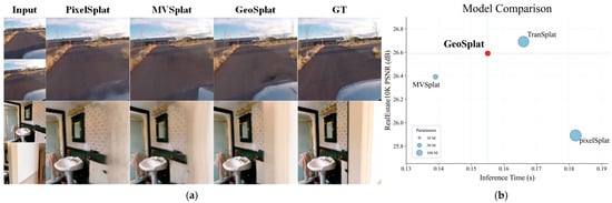
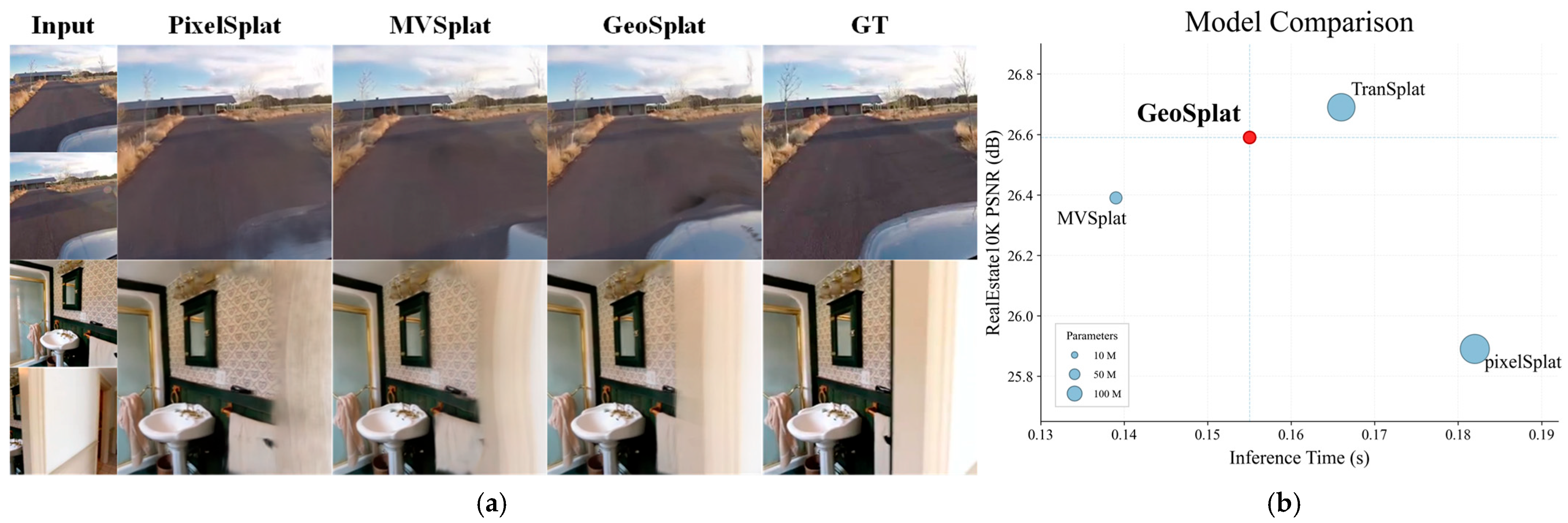
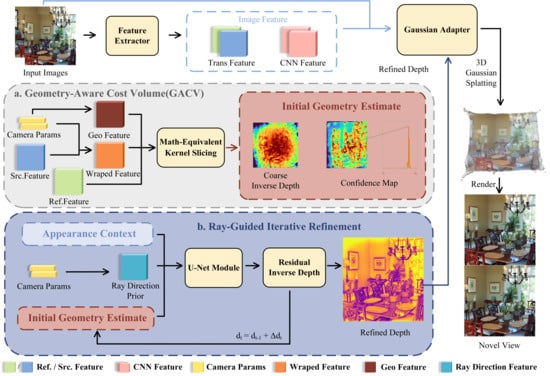
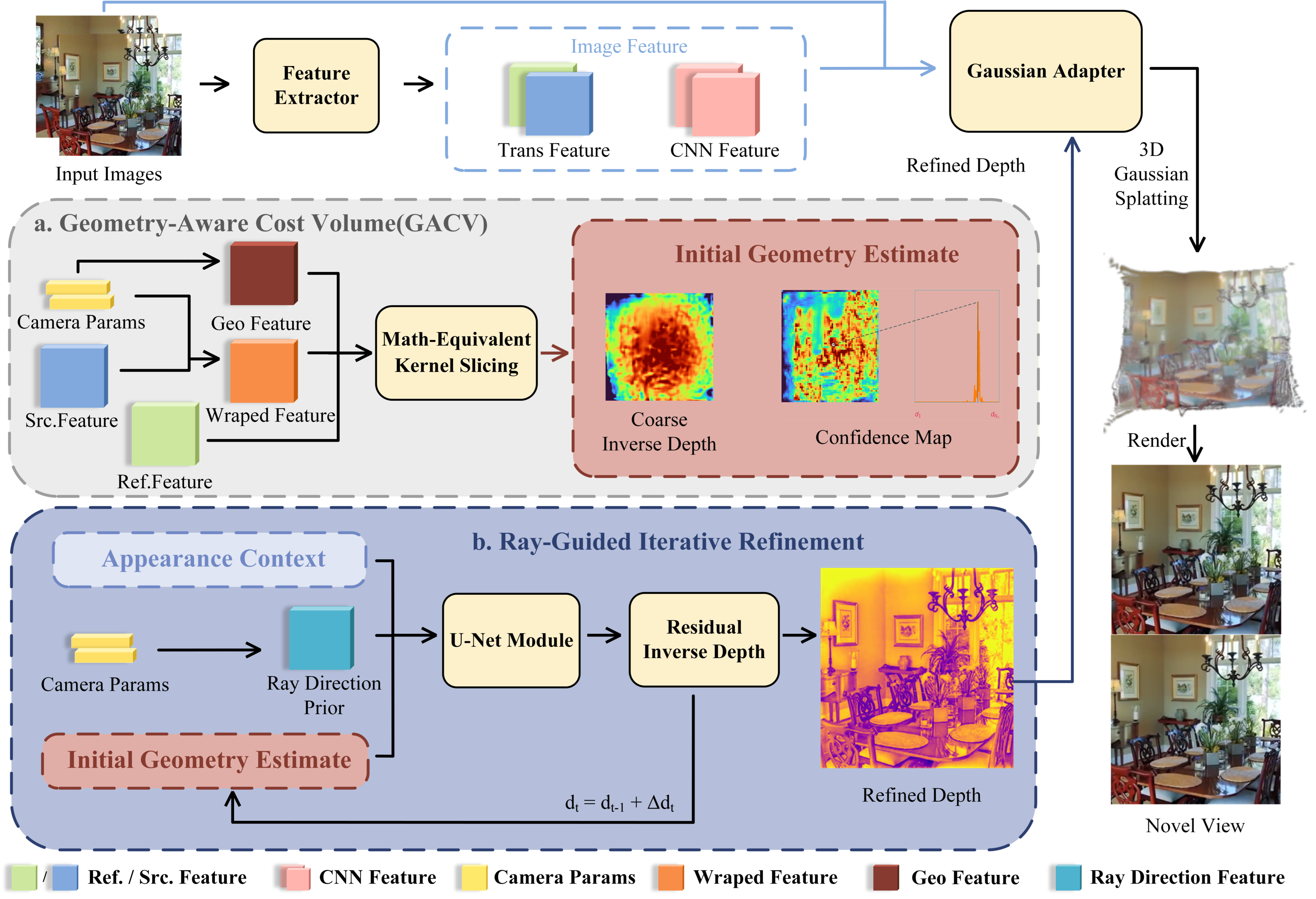
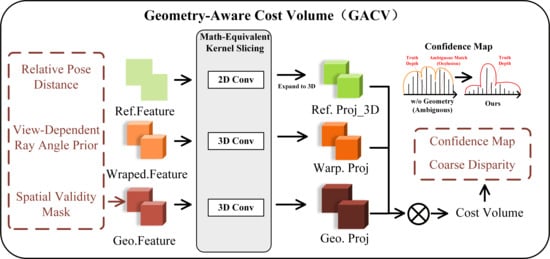
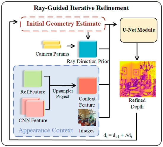
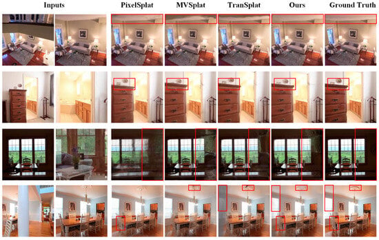
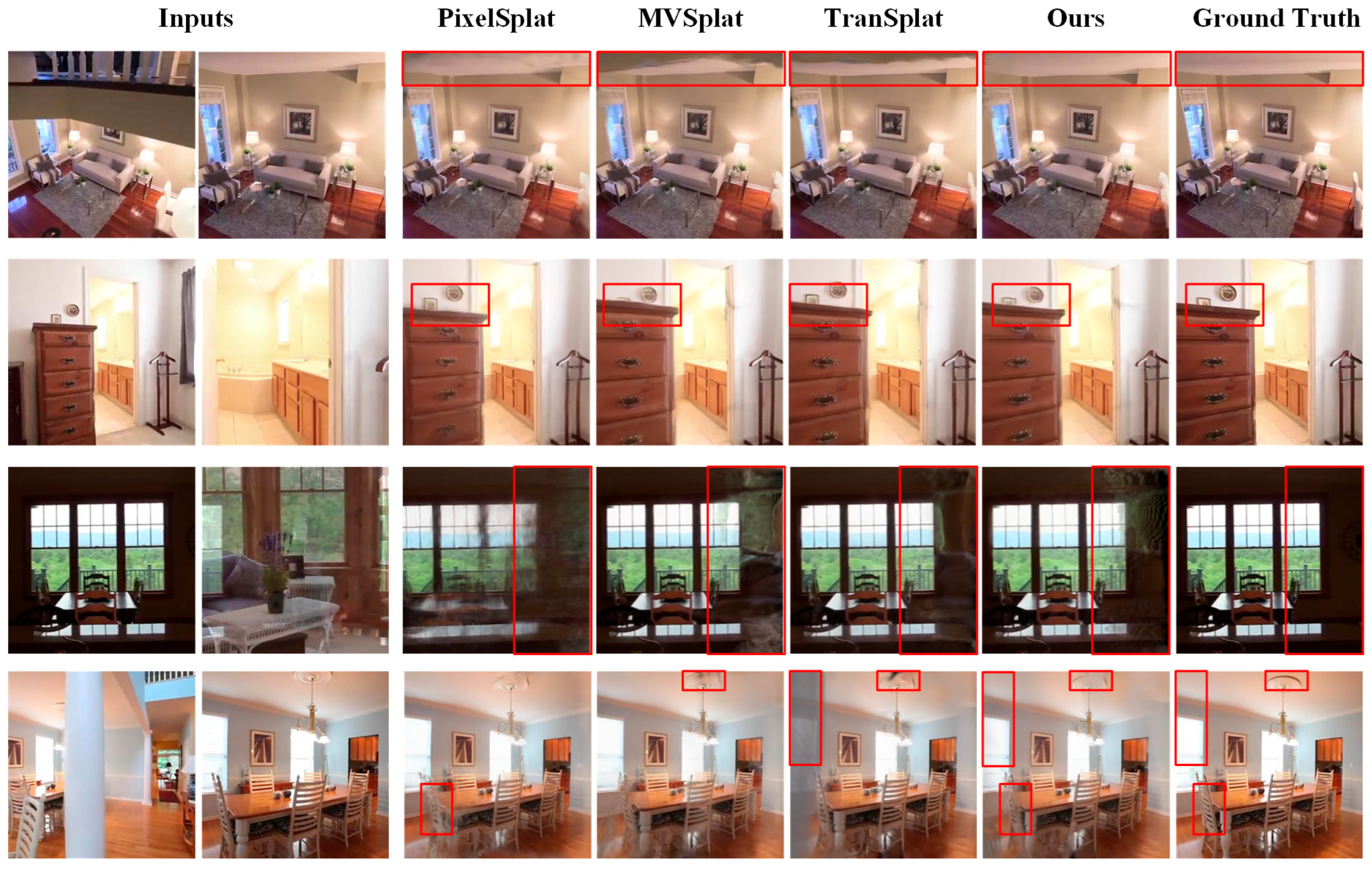
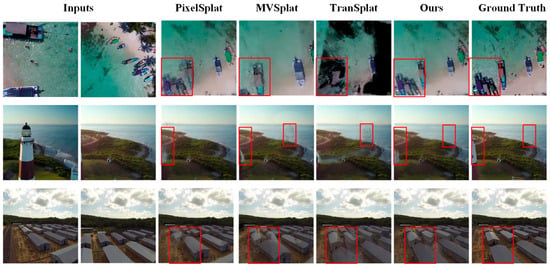
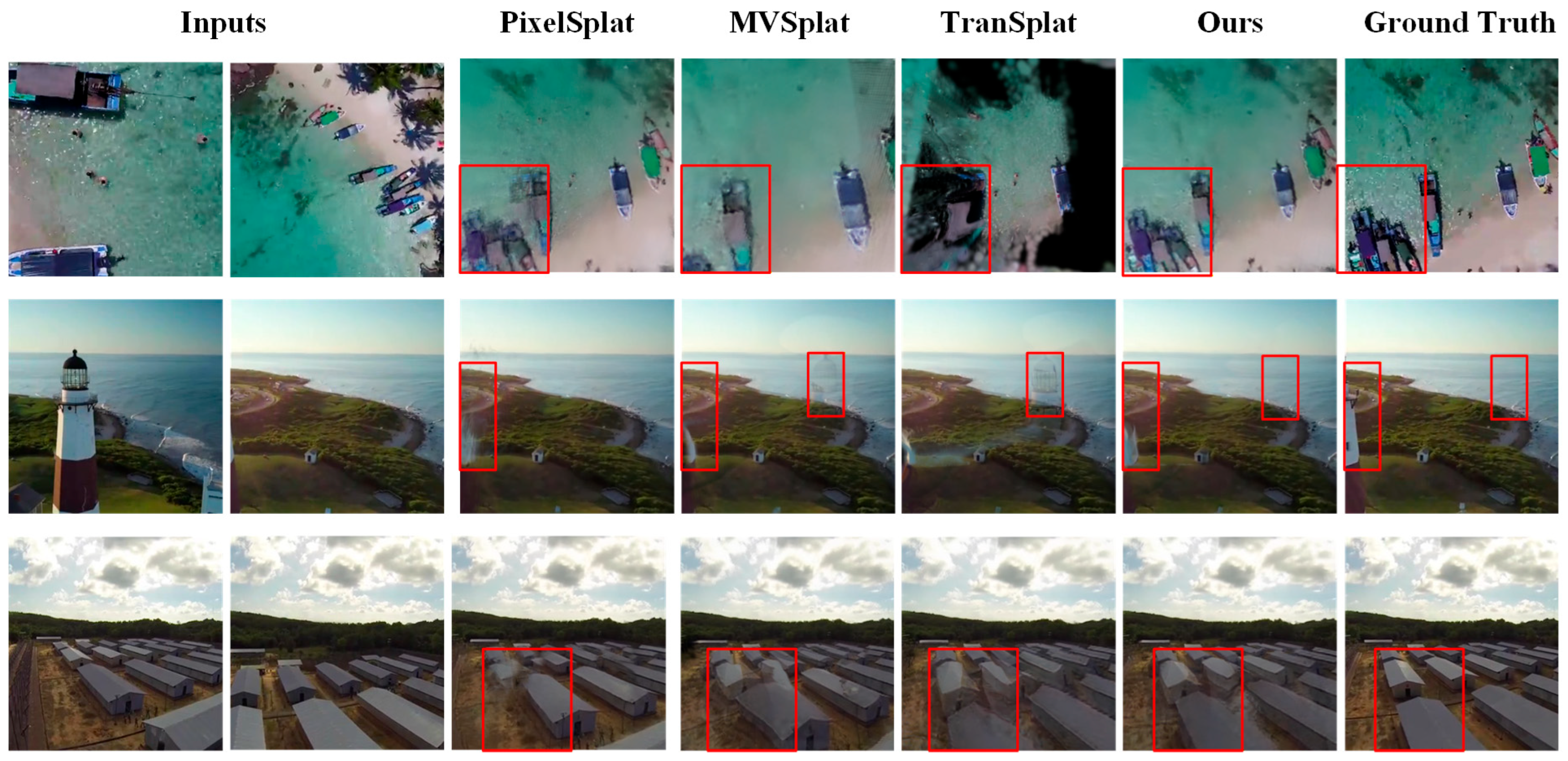
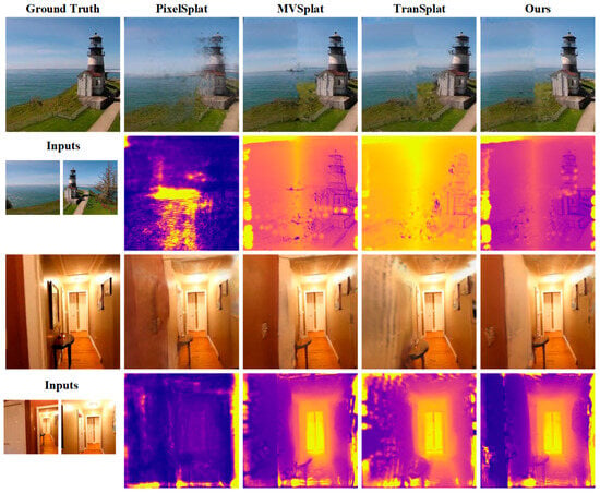
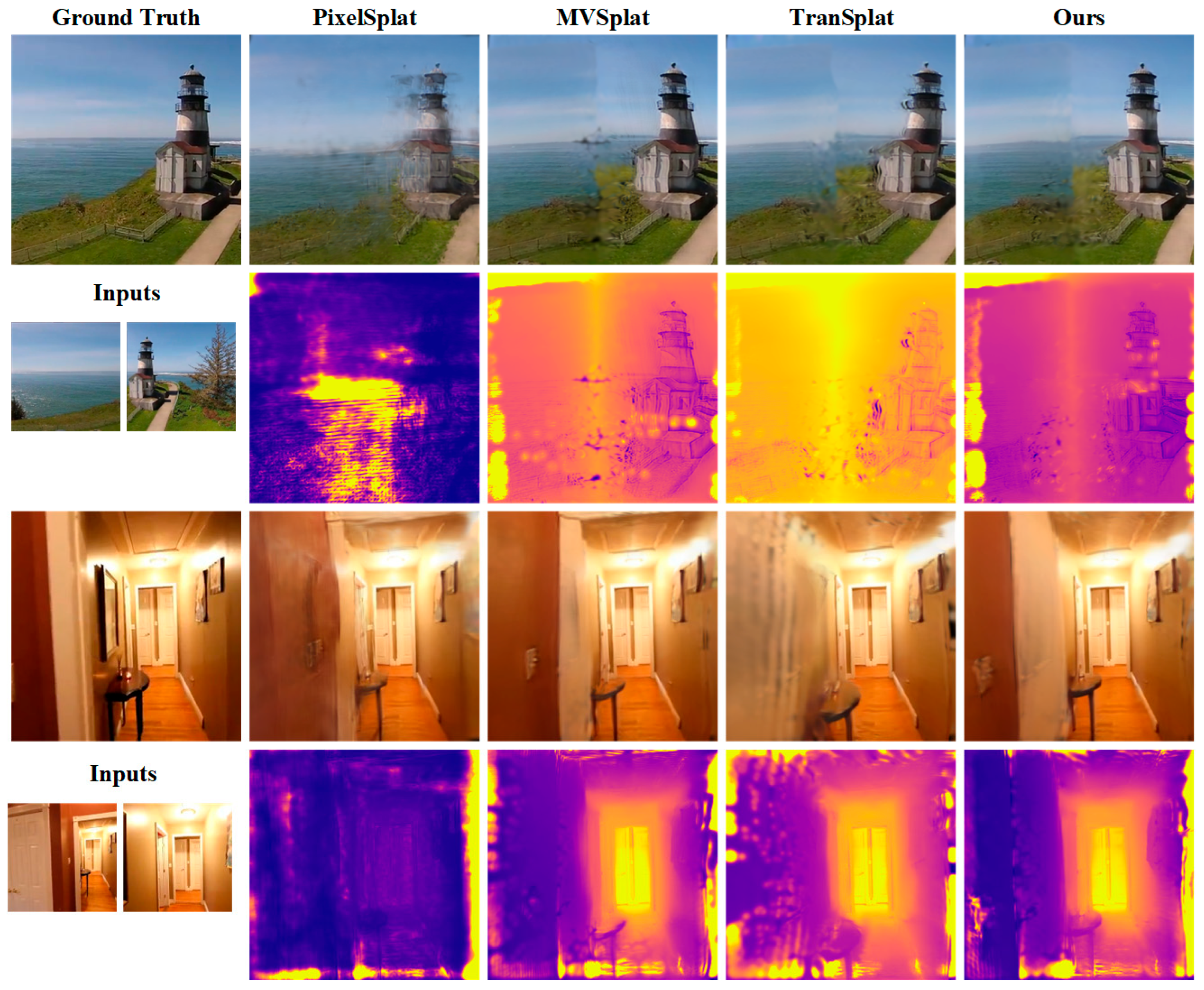
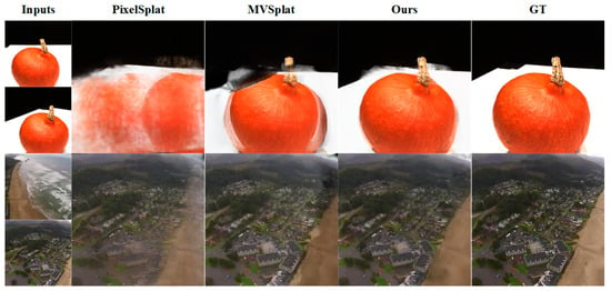
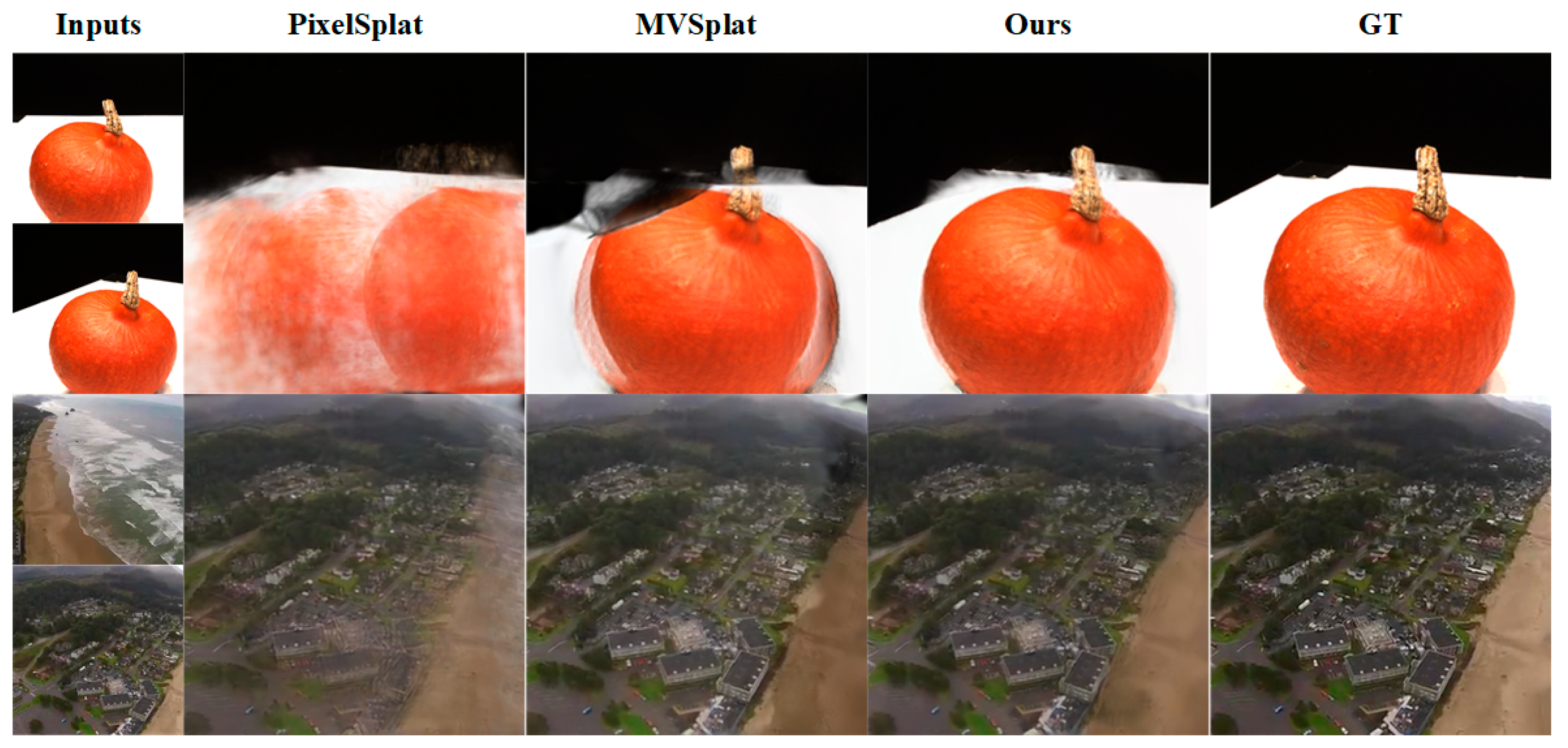
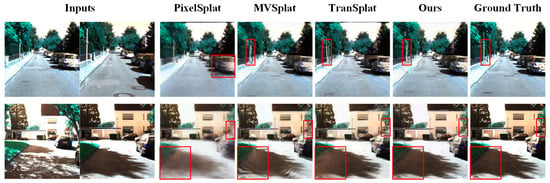
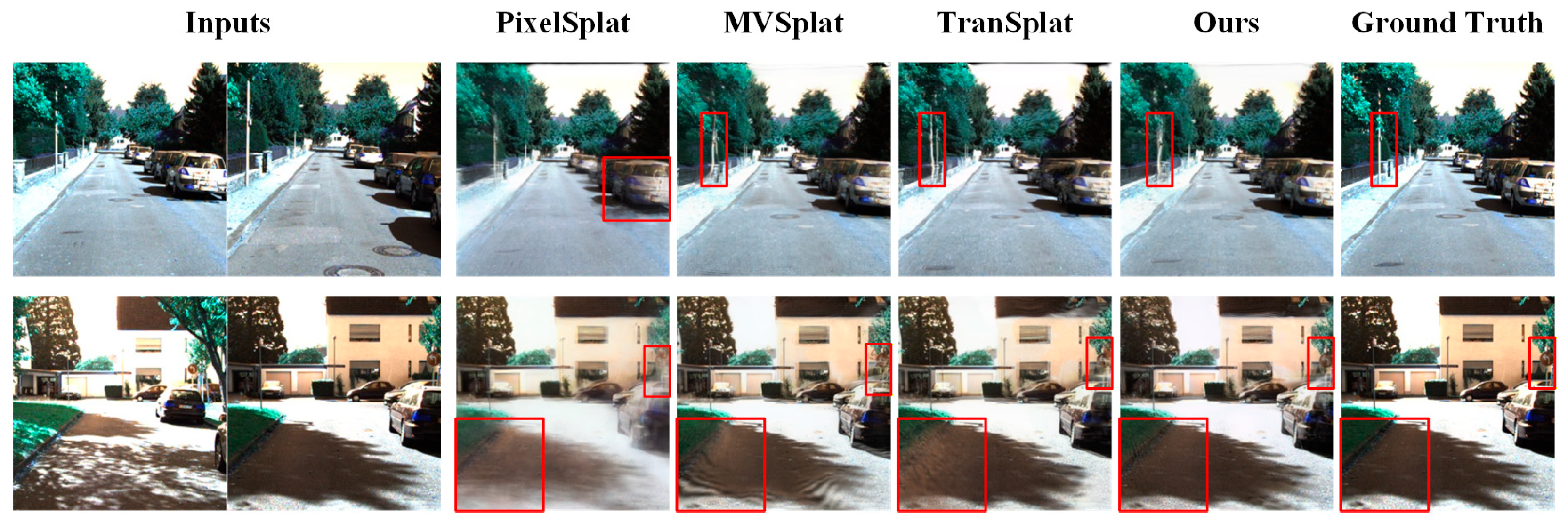
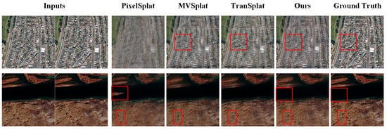
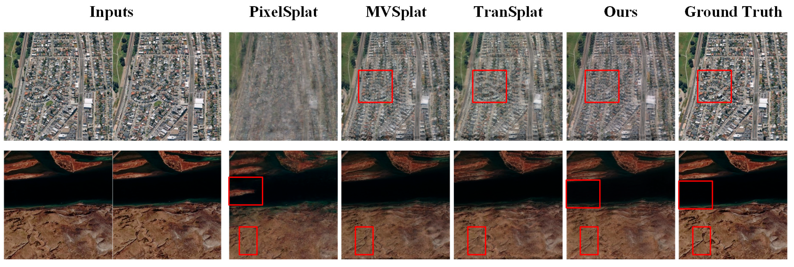
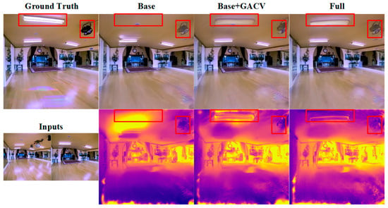
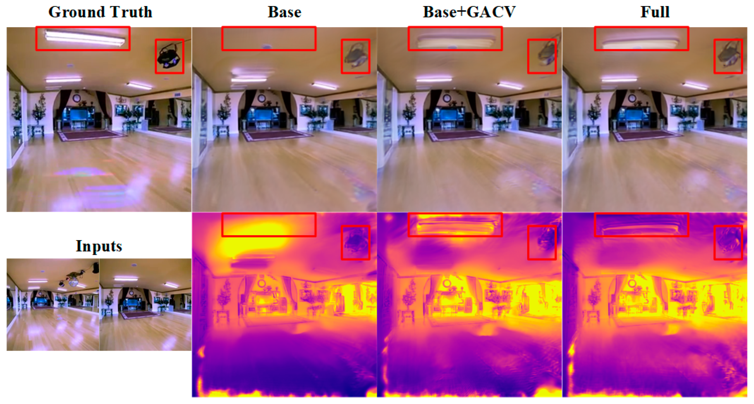

Disclaimer/Publisher’s Note: The statements, opinions and data contained in all publications are solely those of the individual author(s) and contributor(s) and not of MDPI and/or the editor(s). MDPI and/or the editor(s) disclaim responsibility for any injury to people or property resulting from any ideas, methods, instructions or products referred to in the content. |
© 2026 by the authors. Licensee MDPI, Basel, Switzerland. This article is an open access article distributed under the terms and conditions of the Creative Commons Attribution (CC BY) license.