


Abstract
X-ray computed tomography (CT) is widely used in non-destructive testing; however, it exhibits inherent limitations when scanning objects with a large aspect ratio. Computed laminography (CL) provides an alternative solution; nevertheless, due to its distinctive scanning geometry, analytical CL reconstruction methods, such as the filtered back projection (FBP) algorithm, are prone to laminographic and superposition artifacts, thereby degrading image quality. To address this issue, a perspective transformation-based data conversion method (PT-CL-FDK) for cone-beam CL is proposed. Firstly, a virtual detector is introduced, and the perspective transformation relationship between the real and virtual detectors is derived. Secondly, the acquired CL projection data are transformed onto the virtual detector. Finally, the converted projection data are reconstructed using a CL-FDK algorithm. Simulation and real printed circuit board (PCB) experimental results demonstrate that, compared with CL-FBP, the proposed method effectively suppresses superposition artifacts and preserves object boundaries, while significantly enhancing the contrast and resolution of void defects in PCBs.
1. Introduction
Computed tomography (CT) technology, as a non-destructive testing technique, has been widely used in industrial fields [1,2], geological exploration [3], and medical applications [4], among others. Its principle is to visualize internal structures by capturing the attenuation information of X-rays penetrating the sample. However, traditional Cone-Beam CT (CBCT) still faces the following challenges for objects with a large aspect ratio [5,6]: these objects require higher X-ray energy to achieve sufficient penetration, as otherwise the radiation becomes excessively absorbed, which results in incomplete projection data and consequently introduces artifacts in the reconstructed images. To overcome the limitations of traditional CT scanning, the field has developed computed laminography (CL) technology for objects with a large aspect ratio. Different from the geometry of traditional CT where the rotation axis is perpendicular to the X-ray beam, CL introduces a certain tilt angle to reduce the penetration path length of the X-ray within the object with a large aspect ratio, thereby reducing the energy requirement and improving the completeness of the projection data [7]. However, when the tilt angle is too large, it may still cause inter-layer information mixing, resulting in artifacts specific to laminography.
According to the different scanning trajectories, CL can be broadly divided into translation CL [8], rotation CL [9], and swing CL [10]. Among them, rotation CL has become the mainstream CL technology in current research and applications due to its strong adaptability and rich projection information [5]. Therefore, this paper conducts research based on the rotation CL scanning method. In the field of modern CL reconstruction, many scholars have conducted in-depth research on rotation CL technology [11,12]. The methods for rotation CL image reconstruction are mainly divided into two categories: analytical methods and iterative methods. In analytical algorithms, the Feldkamp, Davis, and Kress (FDK) algorithm [13] is a classical representative. It first performs geometric correction and filtering on the cone-beam projection data and then completes the reconstruction through weighted back-projection. However, it should be noted that the standard FDK algorithm framework requires that the line connecting the center of the turntable and the focus of the X-ray source passes through the center of the detector and is perpendicular to the detector plane and the rotation axis [14]. For rotation CL, Yang et al. [12] proposed a filtered back-projection (FBP) method under arc trajectory CL scanning mode (CL-FBP), which performs reconstruction by applying the traditional S-L filter to the original CL data. However, the CL-FBP method does not fully consider the structural characteristics of CL scanning, and its projection data do not strictly meet the requirements of the traditional FBP algorithm. Therefore, Sun et al. [15] proposed a cone-beam CL data conversion method based on projection transformation to obtain the CL projection data required for filtering. Compared with the previous CL-FBP method, this method can effectively reduce artifacts. Additionally, due to the limitations of the physical size of the detector, objects with a large aspect ratio often exceed the field of view (FOV) of the CL system, resulting in truncation artifacts. Fu et al. [16] developed an asymmetric rotational geometry to enlarge the field of view, Zhang et al. [17] adopted a displaced sample stage scanning mode combined with Parker weighting for projection data optimization, and Wang et al. [18] proposed a Two-Step Weighted FBP (TS-FBP) algorithm for truncation artifact correction. These methods effectively solve truncation artifacts but do not address the superposition artifacts inherent in the tilted CL geometry. In contrast, iterative reconstruction techniques, such as the conjugate gradient least squares (CGLS) algorithm [19], have been widely applied to rotational CL due to their ability to flexibly accommodate non-standard geometries and incomplete projection data. For example, Fisher et al. [20] applied the CGLS reconstruction algorithm to a rotational CL scanning configuration, analyzing the causes of image artifacts in cone-beam CL reconstructions and developing correction methods, thereby achieving high-quality reconstruction of projection images under this scanning mode. Subsequently, Wang et al. [11] addressed the problems of projection truncation and Region of Interest (ROI) artifacts that are prone to occur in cone-beam rotation CL scanning for samples with large aspect ratios. They proposed an ROI Conjugate Gradient Weighted Least Squares (ROI-CGWLS) reconstruction method based on ray length and source-detector distance weighting, which significantly improves image contrast and resolution while effectively suppressing ROI artifacts. Furthermore, the incorporation of regularization constraints has proven effective for artifact and noise suppression; starting from total variation (TV) minimization [21], various extensions have been developed, including anisotropic TV (ATV) [22], truncated adaptive-weight TV (TAwTV) [23], and related variants. More recently, Tang et al. [24] proposed an anisotropic adaptive weighted TV (AAwTV) model to mitigate inter-layer aliasing and blurring, while Lu et al. [25] introduced an adaptive weighted dynamically adjusted RTV (AwDaRTV) method to further suppress noise and cone-angle artifacts. Overall, although iterative reconstruction methods provide strong adaptability to complex geometries and incomplete data, their high computational cost and sensitivity to parameter tuning limit their practical deployment; consequently, analytical reconstruction methods still dominate in current industrial applications.
Most commercial AXI systems and planar oblique CT systems employ phantom-based geometric calibration strategies to correct various mechanical errors. In contrast, this work proposes a perspective-transformation-based projection-data conversion method that transforms the actual projection data into an equivalent standard geometry suitable for cone-beam reconstruction, thereby enabling image reconstruction using CL-FDK. Specifically, a virtual detector is first constructed such that the central ray is perpendicular to the detector surface, and the perspective-transformation relationship between the physical detector and the virtual detector is derived. Second, based on the established mapping relationship, the acquired cone-beam CL projection data are transformed onto the virtual detector plane. Finally, the transformed projection data are reconstructed using the CL-FDK algorithm.
This article is structured as follows. Section 2 provides the formulation of the cone-beam CL-FDK algorithm. Section 3 presents the details of the proposed reconstruction method. Our simulation and real-data experimental results are presented in Section 4. Conclusions and discussions are provided in Section 5.
2. Preliminary Knowledge
The core of CL is to reconstruct three-dimensional structures from incomplete projection data. Unlike CBCT, the trajectories of the X-ray source and detector in CL do not cross the central axis of the object but instead are tilted relative to the object. This avoids the requirement for full-angle rotation of large-sized objects and reduces the risk of collision between the source, detector, and object. This geometric design enables CL to significantly reduce X-ray penetration thickness and improve image resolution when inspecting objects with a large aspect ratio such as multi-layer Printed Circuit Boards (PCBs) [9] and Insulated Gate Bipolar Transistors [26].
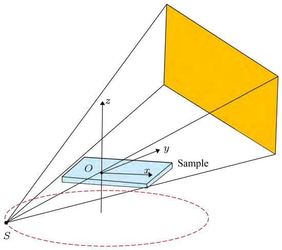
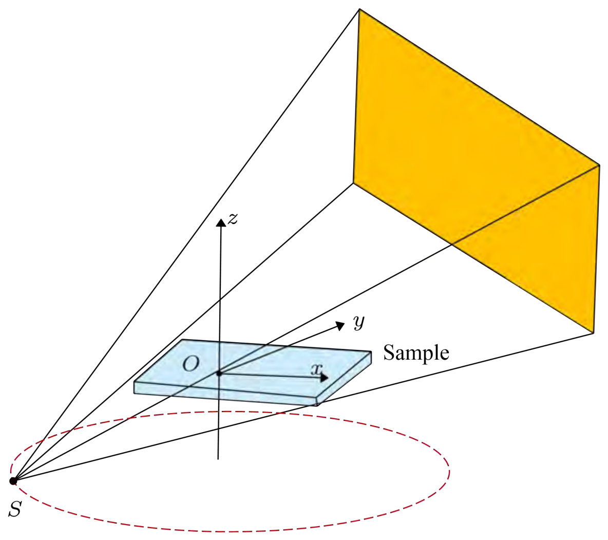
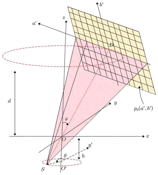
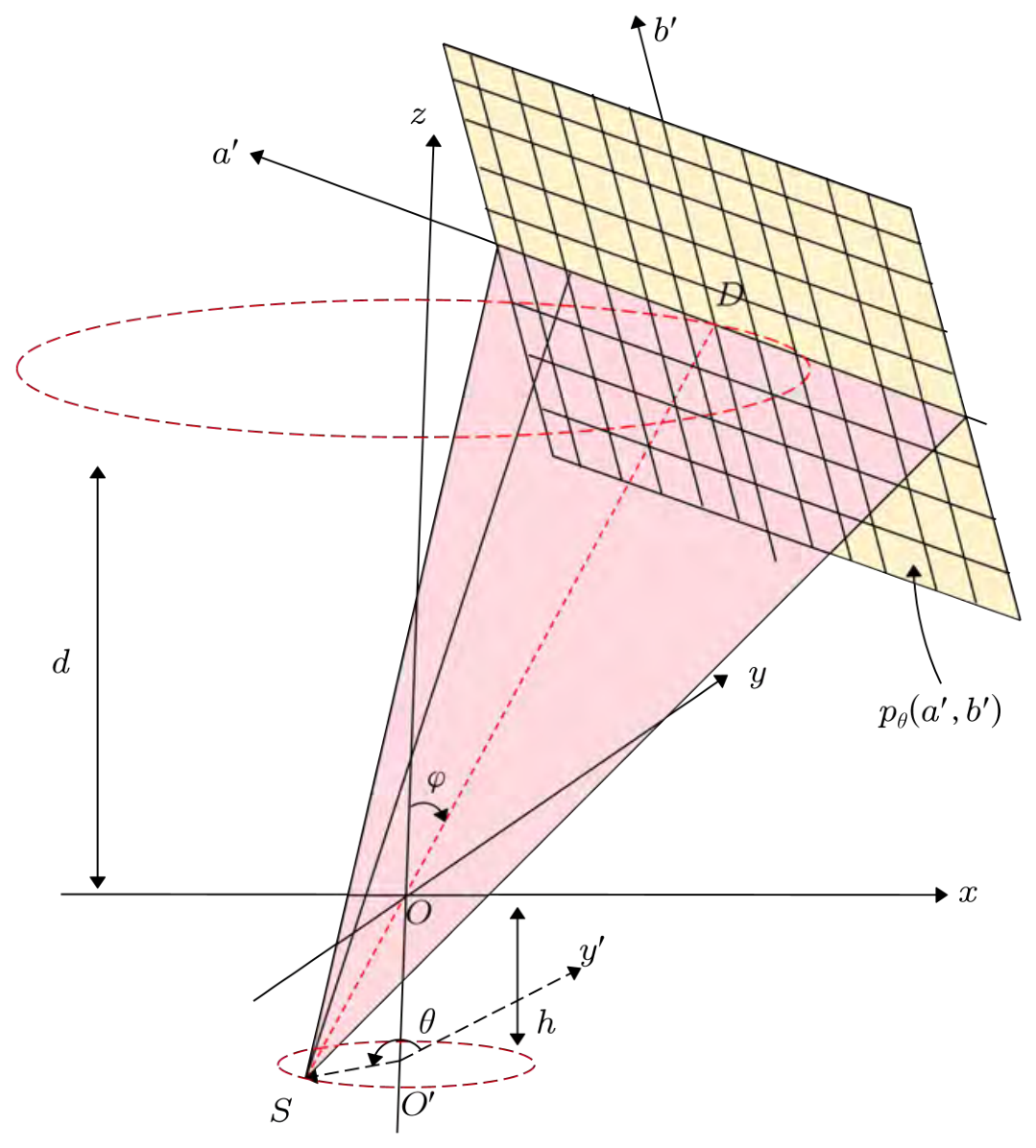
Figure 1 illustrates the rotary CL scanning mode, where the X-ray source and detector rotate synchronously along circular trajectories around the z-axis while the object remains stationary. However, according to the Tuy–Smith condition [27], accurate reconstruction of a point requires that all scanning planes passing through that point intersect the source trajectory plane. The scanning mode shown in Figure 1 does not satisfy the Tuy–Smith condition; therefore, exact reconstruction using a strict analytical back-projection formula is not possible. Figure 2 shows the cone-beam rotary CL scanning geometry with a flat-panel detector. For this scanning mode, Wang et al. [28] introduced an approximate CL-FDK reconstruction algorithm. To simplify the mathematical representation of the geometric projections, a virtual detector is introduced. The projection data on the virtual detector, denoted as , is derived from the actual detector projection data through the scaling relations and . The approximate CL-FDK formula is given as follows:
where
Figure 1.
Schematic illustration of rotary CL scanning.
Figure 2.
The line SD is always perpendicular to and intersects the detector center D. The X-ray source S and the flat-panel detector rotate synchronously along concentric circular trajectories; d is the perpendicular distance from D to the plane, h is the perpendicular distance from S to the plane, the tilt angle is the angle between the z-axis and the central ray SD, and the projection angle is the angle between the projection of the y-axis onto the X-ray source rotation plane and the projection of the central cone beam onto the source plane.
The term represents the weighting applied to the projection data and is the filter function.
3. The Proposed Method
3.1. CL Scanning Geometry
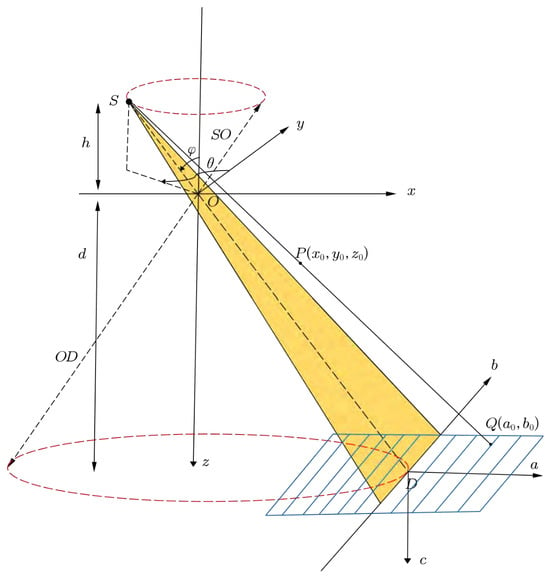
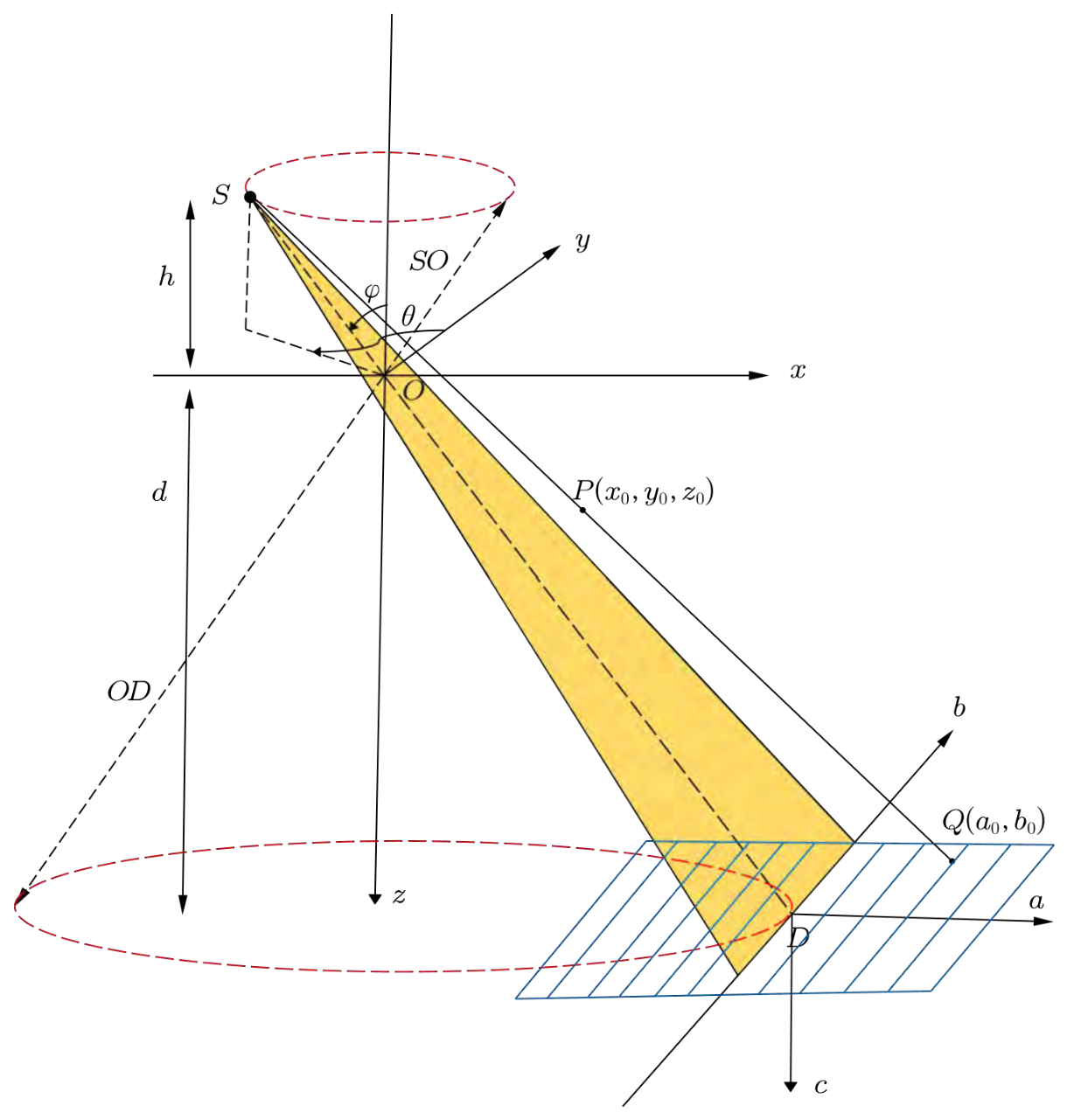
Different from the scanning mode in Figure 2, we focus on the CL scanning mode realized by tilting the source and the detector. Figure 3 illustrates the cone-beam rotary CL with a flat-panel detector. In this configuration, the X-ray source S rotates around the z-axis while the object remains fixed; S and the flat-panel detector rotate synchronously along concentric circular trajectories. The object Cartesian coordinate system is denoted as coordinate system , and the detector coordinate system as coordinate system , where O is the rotation center and D is the detector center. The detector lies in the plane , with its a and b axes parallel to the x and y axes, respectively; while the c-axis is normal to the detector plane. The distance from the X-ray source to the rotation center is , and the distance from the X-ray source to the detector center is . The ray passing through S, O, and D is defined as the central ray. The perpendicular distance from the X-ray source S to the plane is h, and the perpendicular distance from the detector center D to the plane is d. The X-ray source S lies in the plane . The angle is defined as the angle between and the z-axis. The projection angle is defined as the angle between the positive y-axis and the projection of onto the -plane. For an arbitrary point on the object, its projection point on the detector is .
Figure 3.
Cone-beam rotary CL geometry. The X-ray source and the detector rotate synchronously along concentric circular paths, while the object remains stationary. defines the object coordinate system, the detector coordinate system, SO denotes the source-to-center distance, and SD denotes the source-to-detector distance.
Since the geometric scanning modes in Figure 2 and Figure 3 are different, specifically in Figure 3, the central ray SD is not perpendicular to the detector plane; this particular scanning mode renders Equation (1) unsuitable for direct use in approximate reconstruction. Therefore, we propose a method based on perspective transformation to make the projection data satisfy the conditions required by the CL-FDK algorithm, after which the CL-FDK method is applied for reconstruction.
3.2. Perspective Transformation Formula
As illustrated in Figure 3, the circular trajectories of the X-ray source S and the detector center D in the object coordinate system O- can be expressed as
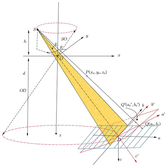
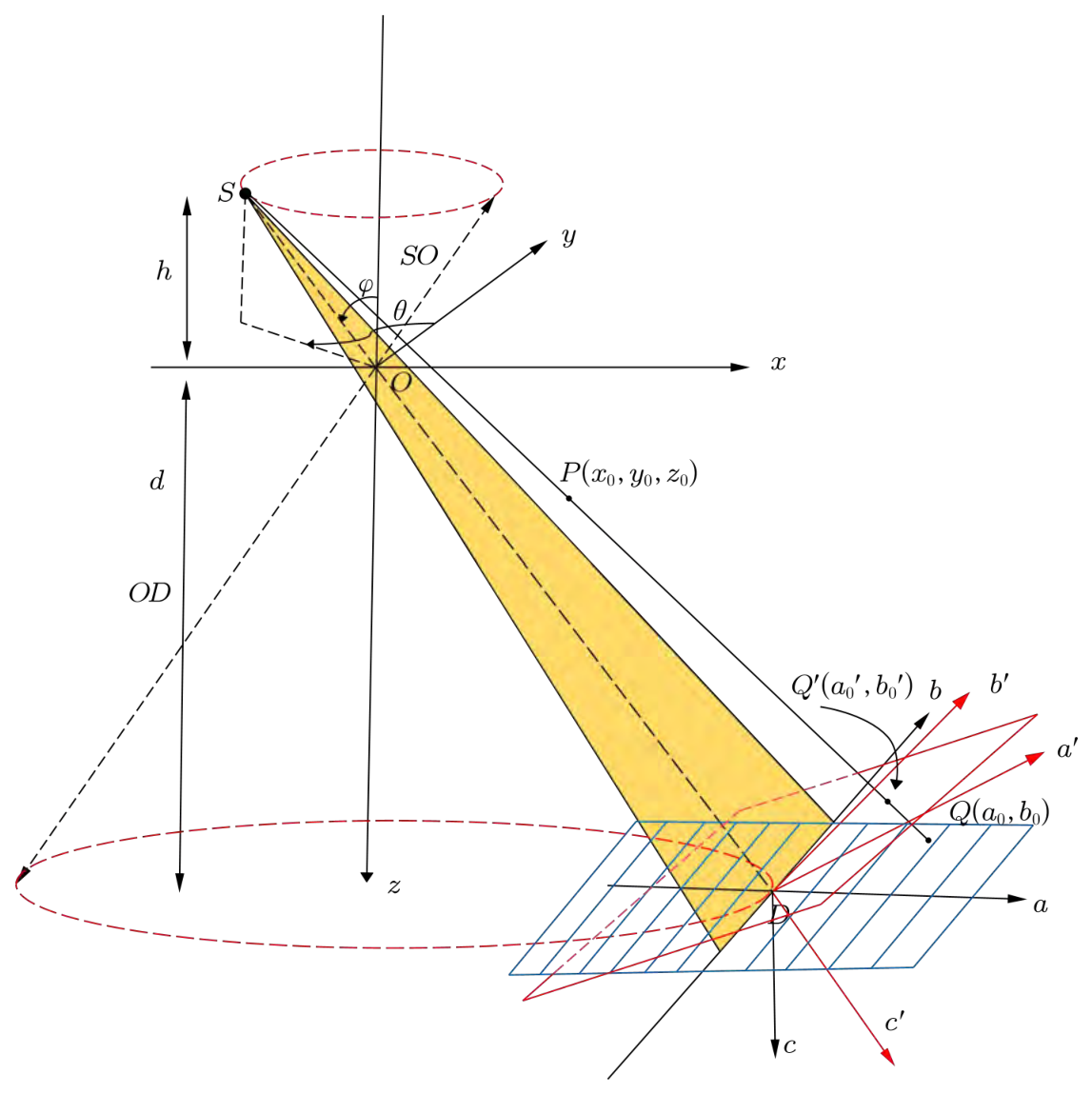
To facilitate subsequent derivations, a virtual detector is introduced, as seen from Figure 4. Let the coordinate system of the virtual detector be denoted as coordinate system , where the detector center coincides with D. The -axis and -axis correspond to the row and column directions of the virtual detector, respectively. This configuration ensures that the central ray is perpendicular to the virtual detector, thereby enabling the application of the CL-FDK reconstruction formula. To describe the transformation between the real and virtual detectors, an intermediate coordinate system is further introduced. The unit normal vector of the real detector is defined as , while the unit normal vector of the virtual detector , is aligned with the direction of . The ray direction vector can be expressed as
Figure 4.
The cone-beam rotary CL with virtual detector: the central ray SD is perpendicular to the virtual detector.
After normalization, we obtain the unit normal vector of the virtual detector
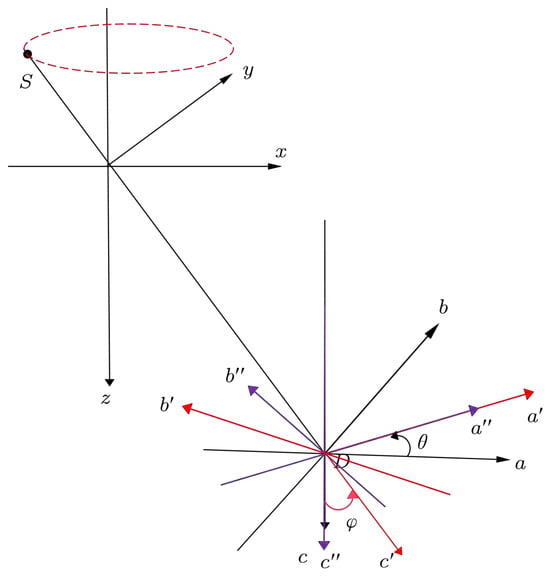
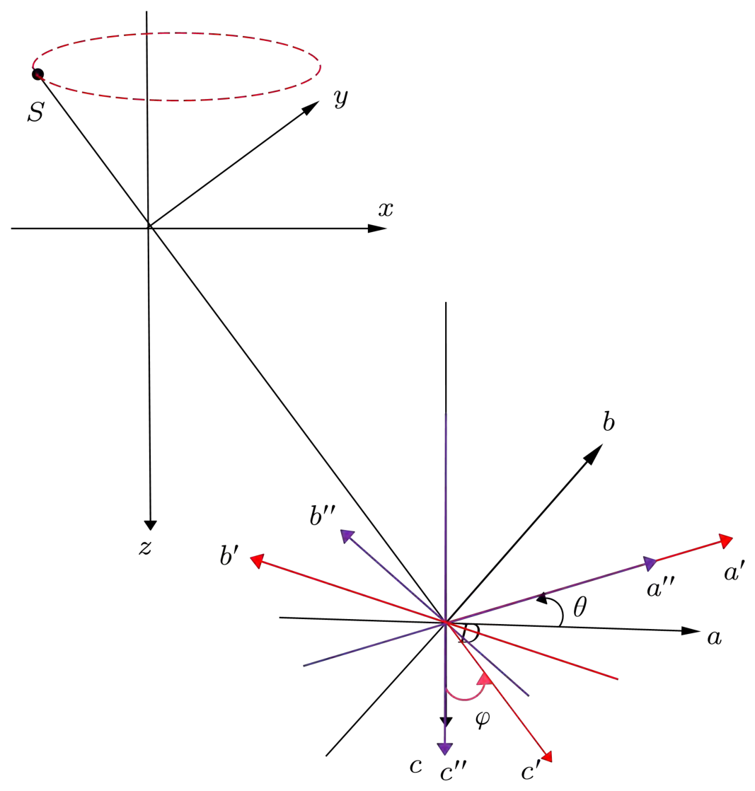
Since the actual detector plane remains parallel to the -plane of the object coordinate system throughout the scan, the detector’s c-axis stays strictly parallel to the object’s z-axis; consequently, the rotation angle around the c-axis in the detector coordinate system is identically the azimuthal angle defined in the object coordinate system . It is precisely this equivalence that dictates the first step when aligning vector with : as illustrated in Figure 5, the real detector coordinate system is first rotated about the c-axis by this same angle (following the right-hand rule), yielding the intermediate coordinate system , and the relation between the coordinate frames can be written as
Figure 5.
The coordinate transformation from coordinate system to coordinate system is performed in two steps: first, coordinate system is rotated about the c-axis by the azimuthal angle to yield the intermediate frame coordinate system ; second, coordinate system is rotated about the -axis by an angle to obtain the virtual detector coordinate system .
Second, with the intermediate coordinate system fixed, the spatial vector is rotated about the -axis by an angle following the right-hand rule to obtain the virtual detector coordinate system. The relationship between the coordinate systems can be written as
Combining Equations (9) and (10), the transformation between the real and virtual detectors can be derived as
Equation (11) characterizes coordinate transformation from the real detector coordinate system to the virtual detector coordinate system . Physically, it integrates the rotational motion of the system and the tilt geometry so that its normal axis is precisely aligned with the central ray . Meanwhile, Equation (11) demonstrates the spatial orientations of the coordinate axes of the virtual detector relative to the world coordinate system , meaning that the unit vector of the virtual detector’s row axis is , the unit vector for the column axis is , and the unit vector for the normal axis is aligned with .
To convert the projection data, a perspective mapping between the real and virtual detector planes must be established. Let P be a point in the object, whose projections on the real, intermediate, and virtual detectors are denoted as , , and , respectively. The goal is to derive the explicit relationship between and .
According to the inverse transformation of Equation (9), the relationship between and can be written as
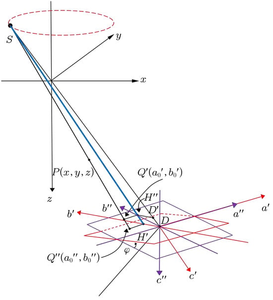
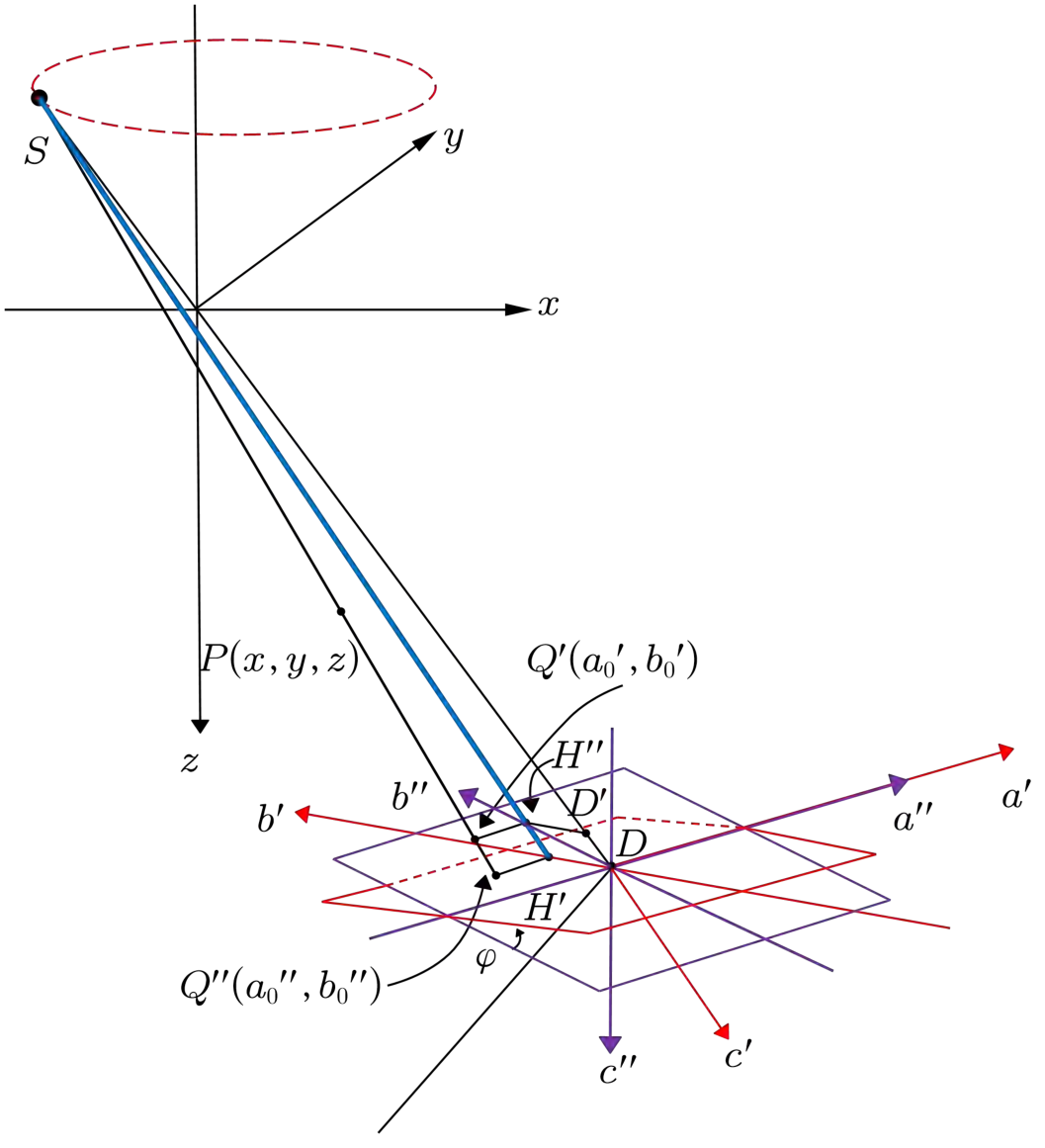
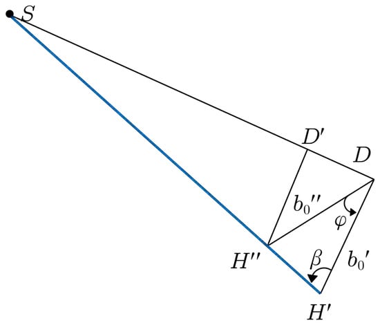
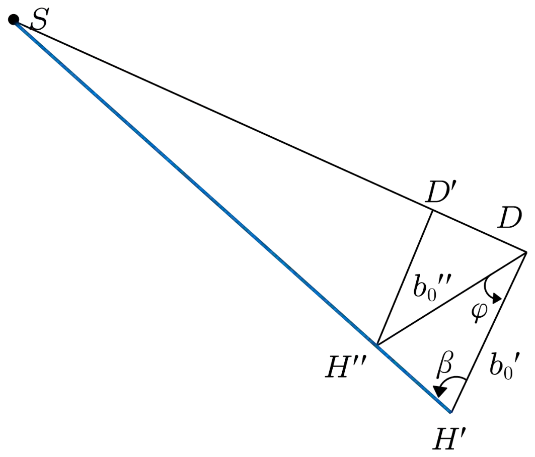
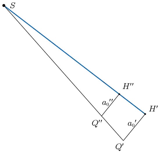
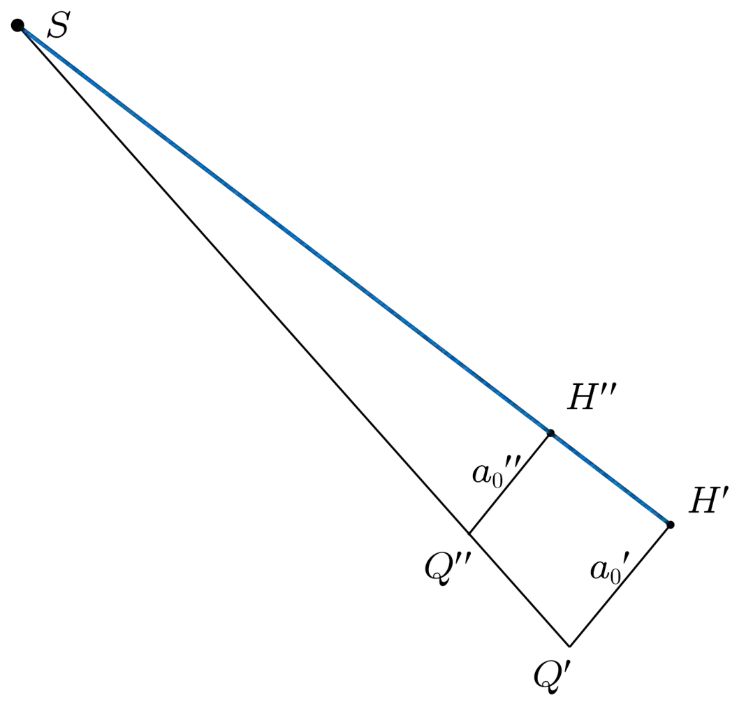
Equations (12) and (13) describe the mapping from the real detector to the intermediate detector. Furthermore, the explicit relationship between and needs to be derived. As illustrated in Figure 6, let denote the projection of onto the -axis, and denote the projection of onto the -axis. A perpendicular is drawn from to , meeting at , and the line segment is also considered. Owing to the perspective projection geometry of X-ray imaging, the points S, , and are co-linear. Figure 7 presents the side view of the geometry shown in Figure 6, providing a clearer representation of the relevant geometric relationships. Let denote the angle between the line segments and . It follows that
Figure 6.
Geometric schematic of the intermediate coordinate system and the virtual detector coordinate system .
Figure 7.
Side view of Figure 6.
Applying the sine theorem to triangle , we have that
For the coordinate along the a-direction, the relationship can be derived from the top view of Figure 6, as illustrated in Figure 8. Based on the similarity of triangles, it follows that
Figure 8.
Top view of Figure 6.
Furthermore, the ratio between and can be expressed as
By combining Equations (12), (13), (16), and (20), the inverse perspective mapping from the virtual detector to the real detector can be obtained as
Equations (21) and (22) establish the explicit coordinate transformation relationship between the virtual detector and the real detector. Based on this perspective mapping relationship, the acquired projection data on the real detector can be converted into the corresponding projection data on the virtual detector plane. Since the virtual detector is constructed by aligning its normal direction with the central ray, the converted projection data satisfy the geometric conditions required by the CL-FDK formulation.
3.3. Conversion and Reconstruction of Projection Data
For the numerical experiment, a uniform sampling grid is defined on the virtual detector. Assuming both detectors share the same resolution and pixel size , the physical coordinates of the sampling points are given by
These coordinates are further converted into pixel indices:
Since are generally non-integer, bilinear interpolation is employed. During the projection conversion process, some mapped coordinates may fall outside the valid detector range due to the perspective transformation. For sampling points beyond the valid detector range, no measured projection information is available. Therefore, these points are assigned zero values during the projection conversion process. Let the real projection data be denoted as , and the converted data on the virtual detector as ; then, we have that
where denotes the bilinear interpolation operator. The actual projection data are converted into the equivalent projection data via that satisfy the standard cone-beam CL geometry. Therefore, the CL-FDK reconstruction formula can be directly applied. The corresponding reconstruction expression is given as
where
The formula describes the following steps:
- denotes the projection data obtained by use of Equation (29) to transform the real projection data ;
- Weighting the projection data by ;
- Filtering each row of the weighted projection data;
- Performing backprojection on the filtered projection data across angles .
It should be pointed out that this algorithm struggles to completely avoid the generation of superposition artifacts during the reconstruction process. Compared to the standard FDK algorithm used in conventional cone-beam scanning, such artifacts are more pronounced under the current geometric configuration, primarily due to the non-standard imaging geometry formed by the tilted detector and the X-ray source. Owing to the inherent geometric limitations of the CL scanning mode, these artifacts are fundamentally difficult to eliminate entirely, and effective correction methods are still lacking. Nevertheless, for some plate-like specimens, this algorithm retains certain practical value. In some reconstructed slices, the impact of artifacts is relatively weak, which can support basic defect identification requirements in industrial non-destructive testing.
4. Simulation and Real Data Experimental Results
4.1. Simulation Data Experimental Results
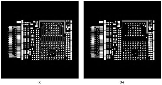
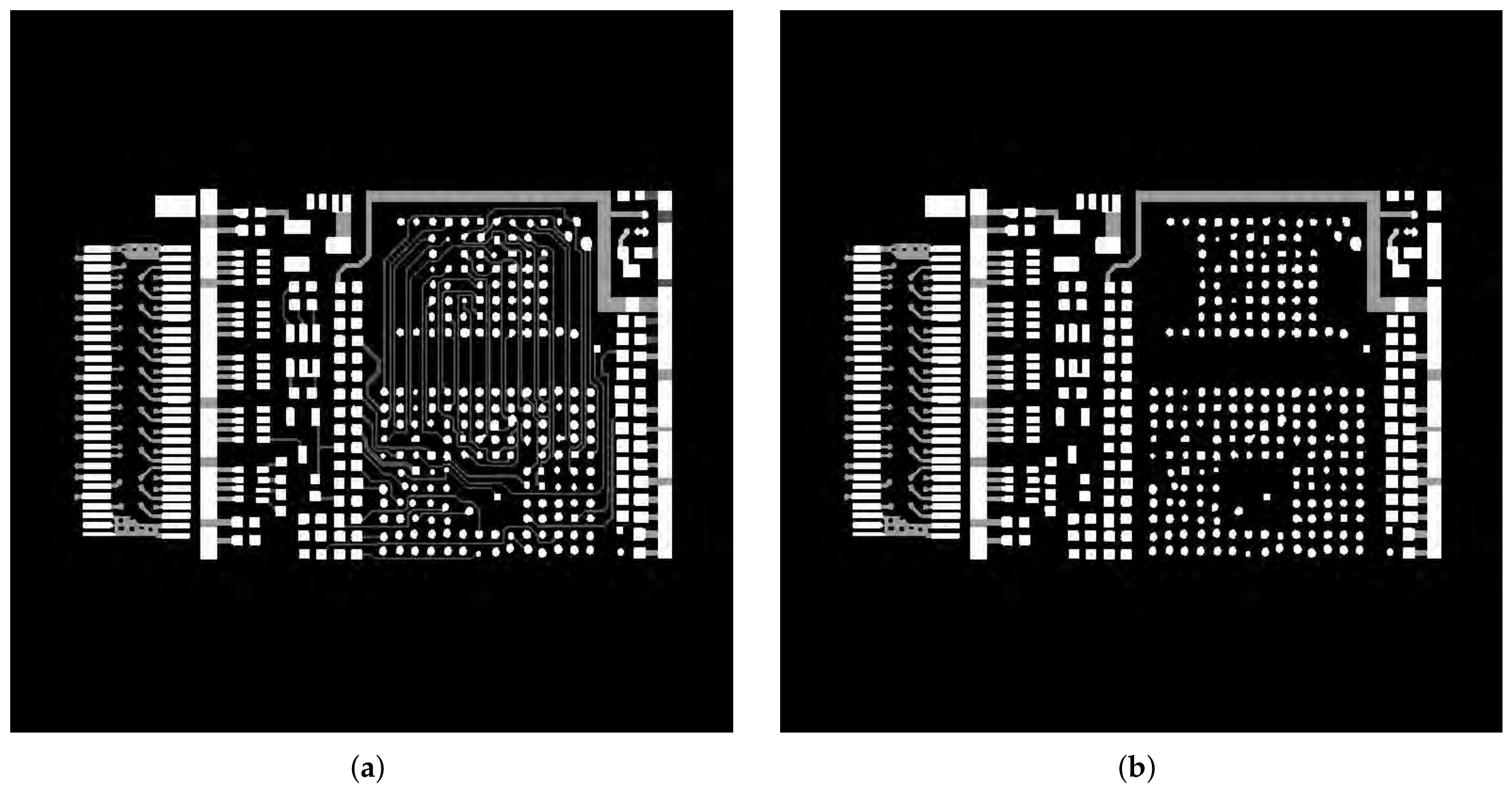
To validate the effectiveness of the proposed PT-CL-FDK method, a simulated PCB phantom is employed. The phantom size is 768 × 768 × 16. The CL-FBP method implemented based on the ASTRA-2.1 toolbox [29] is used for comparison. Both the CL-FBP method and the proposed PT-CL-FDK method use the same simulated projection data acquired under identical scanning geometry conditions. Specifically, the CL-FBP method directly reconstructs the projection data according to the original CL geometry, whereas the proposed PT-CL-FDK method first converts the measured projections onto a virtual detector through the perspective transformation described in Section 3 and then uses CL-FDK reconstruction. The scanning geometry parameters are summarized in Table 1, Figure 9 shows the slices at the 3rd and 7th layers of the phantom.
Table 1.
Simulation parameters of the PCB phantom experiment.
Figure 9.
A simulation PCB phantom. (a) The 3rd slice. (b) The 7th slice.
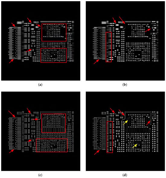
The reconstruction results obtained using the CL-FBP method and the proposed PT-CL-FDK method are presented in Figure 10, for the 3rd slice and 7th slice. The first row shows the CL-FBP reconstruction results, and the second row shows the PT-CL-FDK reconstruction results. The first column corresponds to the 3rd slice, and the second column corresponds to the 7th slice. From these results (highlighted by red arrows and boxes), it can be observed that the proposed PT-CL-FDK method improves the visibility of certain fine structural features, particularly the boundaries of circuit patterns. However, due to the inherent limitations of the CL geometry, this improvement is more evident in relatively homogeneous planar regions, where edges are better preserved than interior areas. Some superposition artifacts remain (indicated by yellow arrows). The experimental results indicate that the PT-CL-FDK method offers practical advantages in certain application scenarios.
Figure 10.
Reconstruction results of simulated data using CL-FBP and PT-CL-FDK: (a) 3rd slice of CL-FBP; (b) 7th slice of CL-FBP; (c) 3rd slice of PT-CL-FDK; (d) 7th slice of PT-CL-FDK.
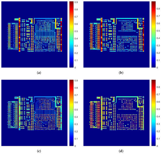
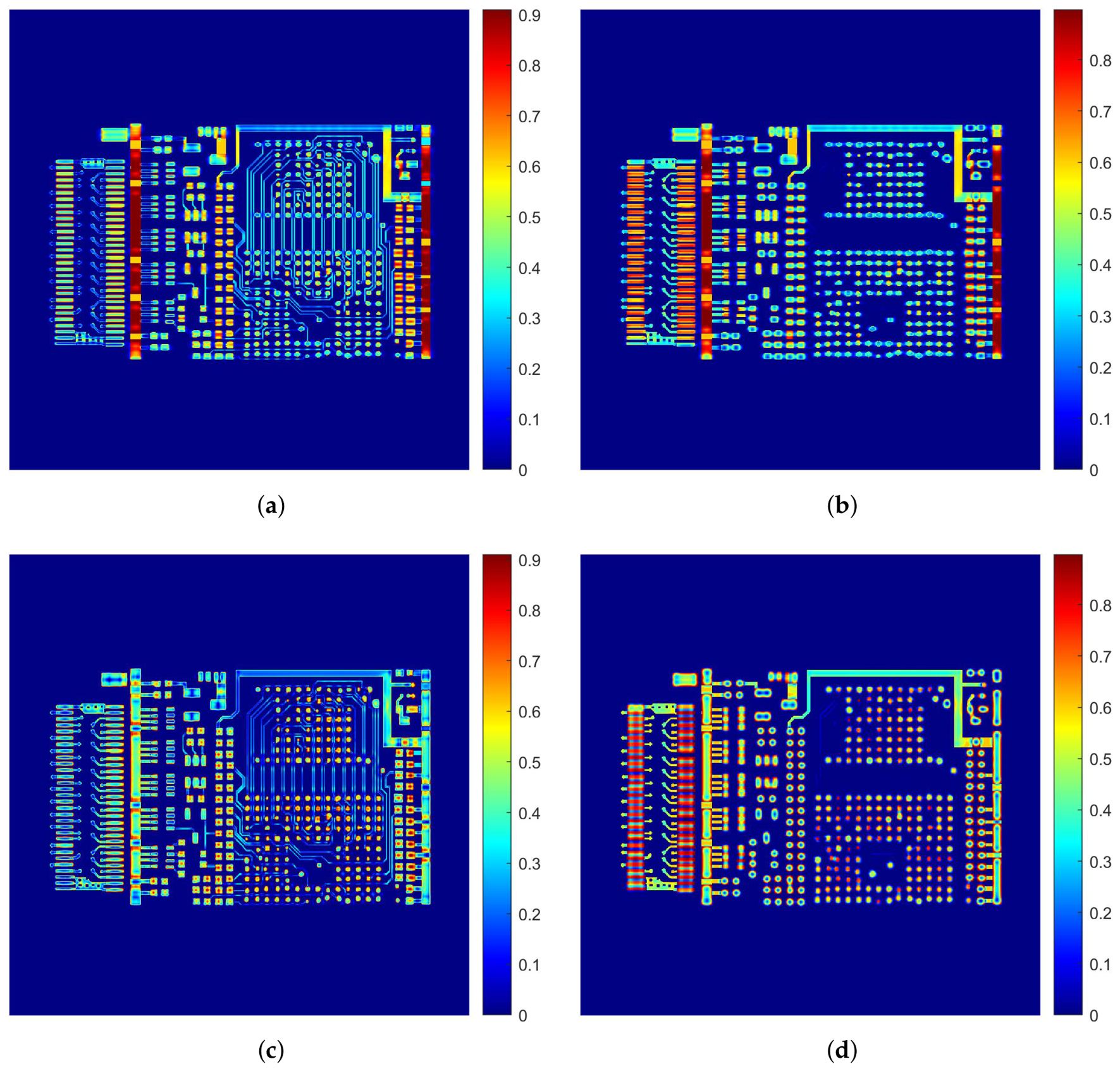
Based on the quantitative evaluation metrics, including root mean square error (RMSE) [30], peak signal-to-noise ratio (PSNR) [31], and structural similarity index (SSIM) [32], together with a visual qualitative assessment, the following observations can be made. The overall average metrics are reported in Table 2. The PT-CL-FDK method outperforms CL-FBP in all three average metrics (RMSE: 51.93 vs. 54.02; PSNR: 13.83 dB vs. 13.49 dB; SSIM: 0.8214 vs. 0.8180), indicating an overall improvement in reconstruction quality. For the individual slices reported in Table 3, the performance of the two methods varies across different slices. For Slice 3, CL-FBP achieves a lower RMSE (54.95 vs. 57.89) and a higher PSNR (13.33 dB vs. 12.88 dB) than the proposed PT-CL-FDK method, indicating better pixel-wise reconstruction accuracy for this particular slice. In contrast, PT-CL-FDK achieves a slightly higher SSIM (0.8236 vs. 0.8055), suggesting better preservation of structural information. In slice 7, the proposed method demonstrates superior performance in two out of three metrics, attaining a lower RMSE (52.23 vs. 52.97) and a higher PSNR (13.77 dB vs. 13.65 dB) compared to the CL-FBP method. Nonetheless, its SSIM is moderately lower than that of CL-FBP (0.8012 vs. 0.8310). Notably, while the quantitative results for slice 3 favor the CL-FBP method, visual comparison indicates that PT-CL-FDK preserves certain structural boundaries more clearly, as illustrated in Figure 10. To further visualize the differences between the two reconstruction methods, Figure 11 presents the absolute difference maps for the 3rd and 7th slices, computed with respect to the ground truth. A blue region indicates that the reconstructed attenuation value closely matches the true physical density, while a red region indicates a large deviation. As can be clearly observed from Figure 11, for the 3rd slice and 7th slice, the PT-CL-FDK difference maps exhibit noticeably darker blue regions (smaller errors) and fewer red regions (large errors) compared to the CL-FBP difference maps, particularly near the edges of some edge features.
Table 2.
Average quantitative results over the 16 reconstructed slices.
Table 3.
The quantitative results of the reconstructed images.
Figure 11.
Difference maps of the reconstructed simulated PCB phantom:. (a) 3rd slice of CL-FBP; (b) 7th slice of CL-FBP; (c) 3rd slice of PT-CL-FDK. (d) 7th slice of PT-CL-FDK.
4.2. Real Data Experimental Results
To validate the effectiveness of the proposed PT-CL-FDK method, we evaluate it on two real PCB projection datasets. For both datasets, all experiments are performed using identical parameters. For comparison, the CL-FBP method implemented in the ASTRA-2.1 toolbox [29] is used. Both the CL-FBP method and the proposed PT-CL-FDK method use the same measured projection data acquired under identical scanning geometry conditions. The scanning geometry parameters are summarized in Table 4.
Table 4.
Real experimental parameters of PCB datasets.
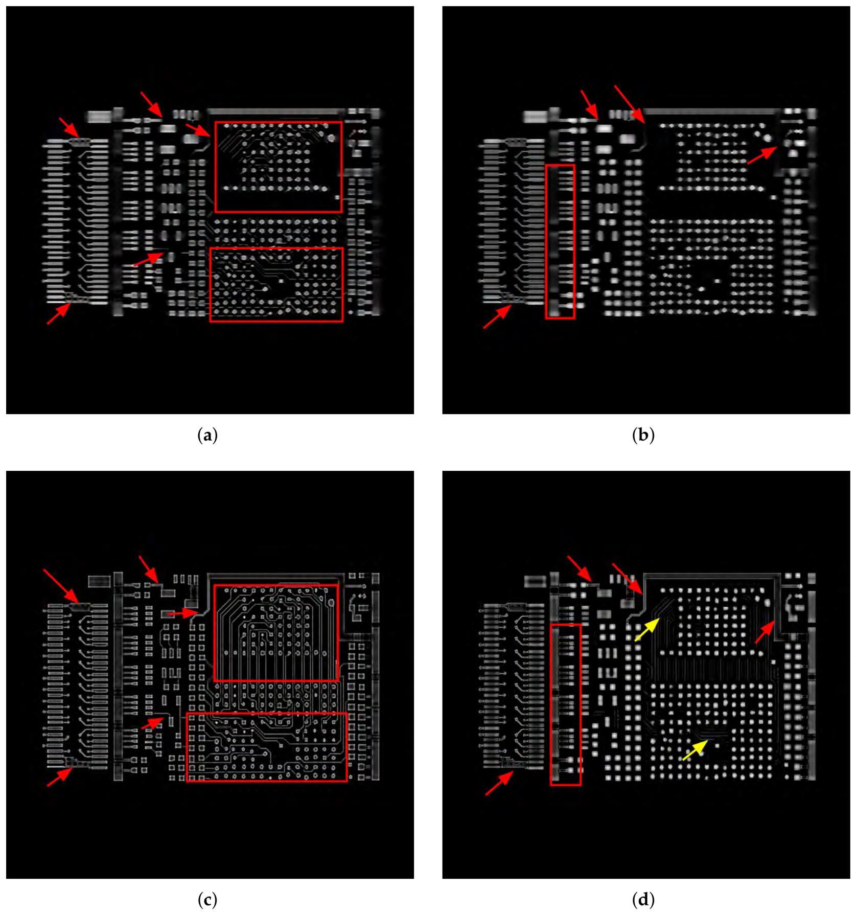
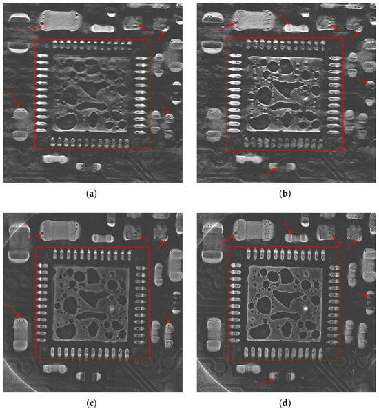
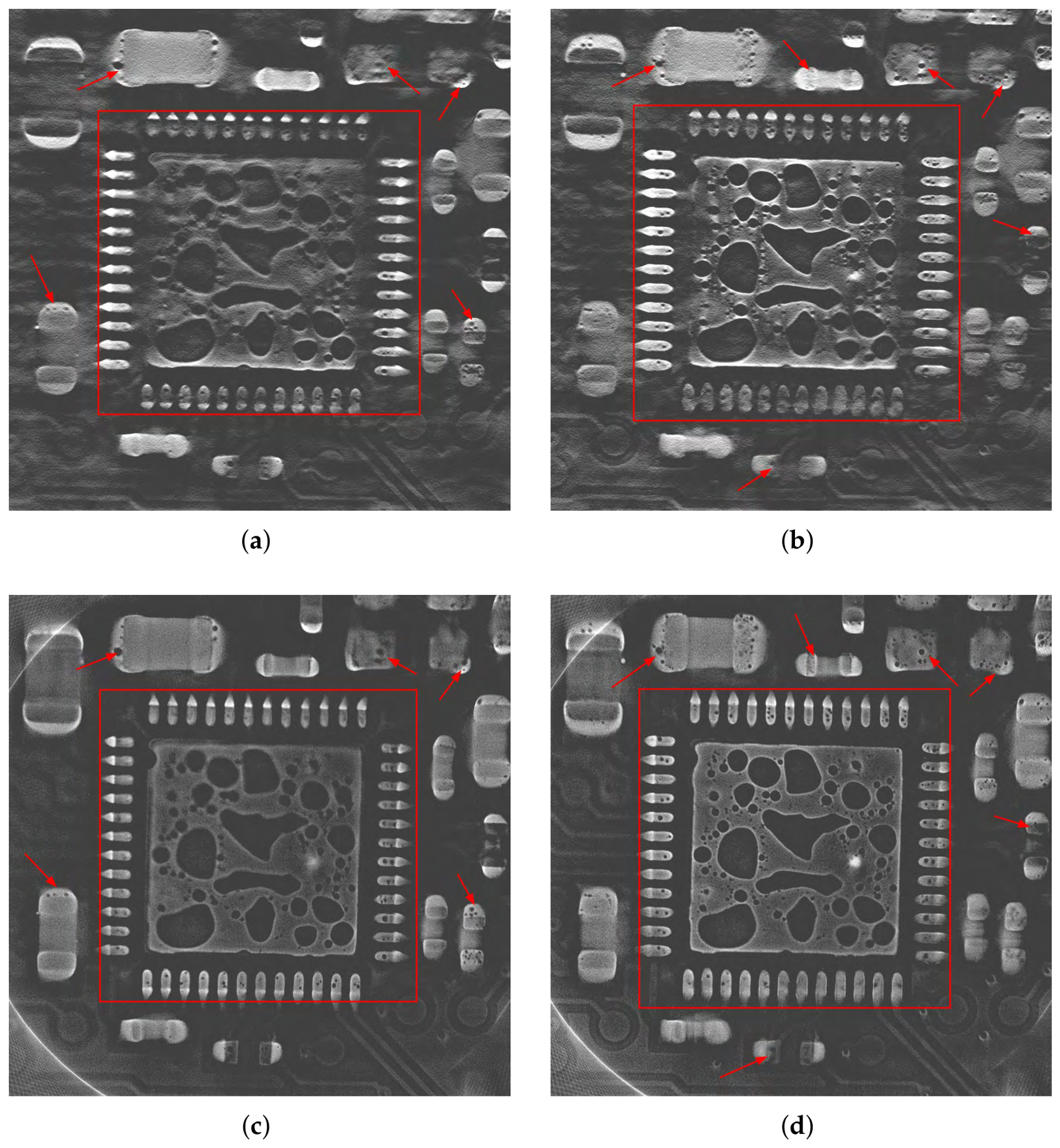
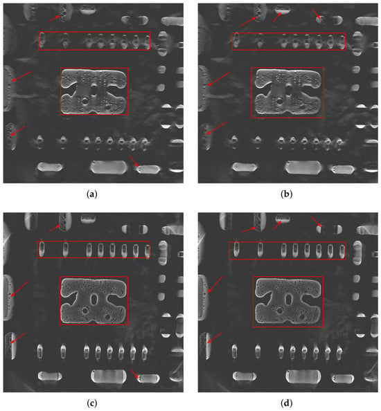
The reconstruction results obtained using the CL-FBP method and the proposed PT-CL-FDK method for the first real dataset are presented in Figure 12, for the 67th slice and for the 73rd slice of the reconstructed volume. For the 67th and 73rd slices, the CL-FBP algorithm fails to clearly reconstruct the rectangular boundaries (indicated by red rectangles), whereas the proposed PT-CL-FDK method not only effectively restores them but also significantly reduces aliasing artifacts. Moreover, for the void defects attached to the surrounding area, the CL-FBP reconstruction results exhibit blurring and obvious superimposition artifacts, while the PT-CL-FDK method effectively suppresses them, allowing the edge contours of tiny voids to be clearly resolved (indicated by red arrows).
Figure 12.
Reconstruction results of the first real data using CL-FBP and PT-CL-FDK: (a) 67th slice of CL-FBP; (b) 73rd slice of CL-FBP; (c) 67th slice of PT-CL-FDK; (d) 73rd slice of PT-CL-FDK.
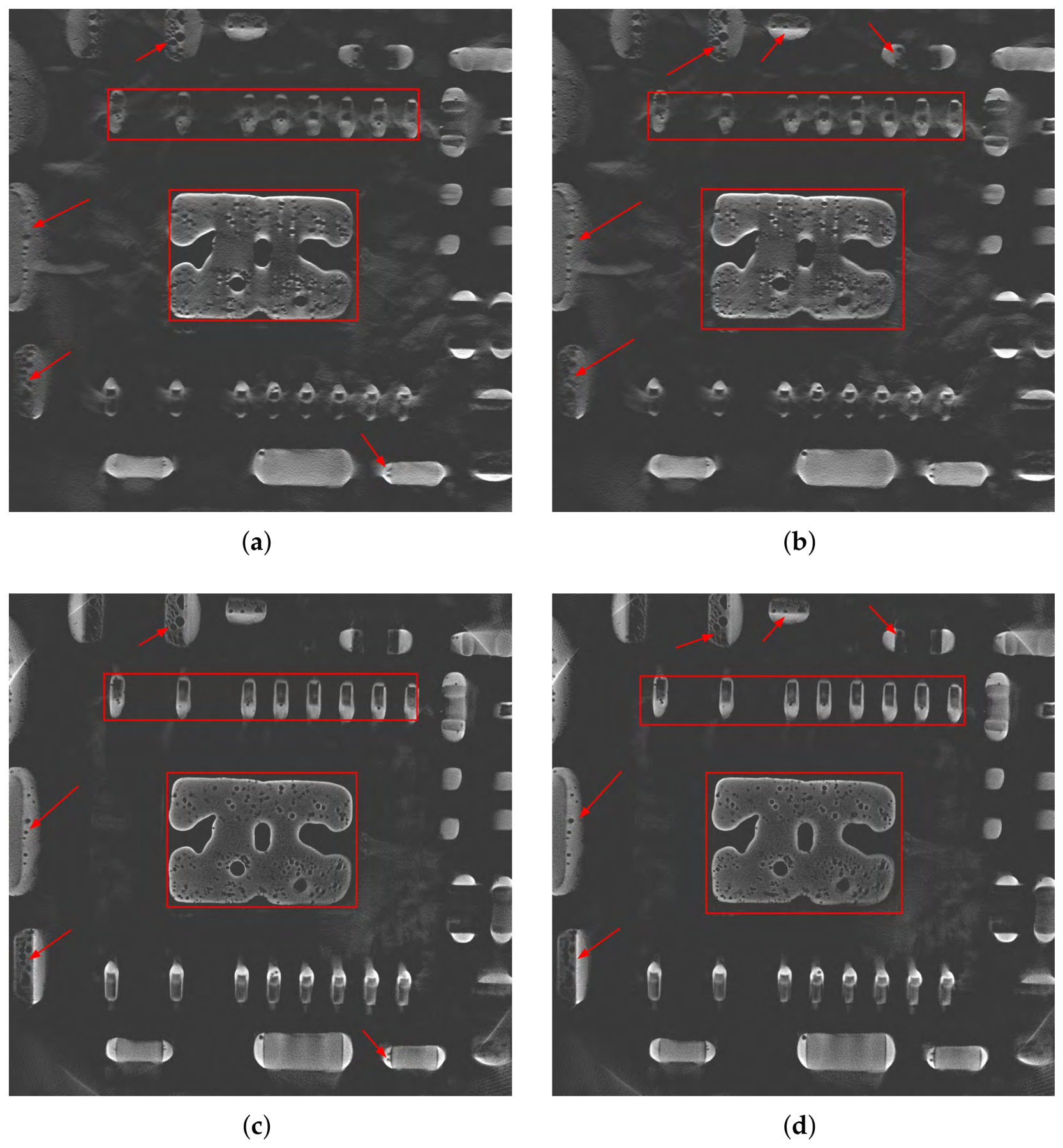
Figure 13 presents the reconstruction results obtained using the CL-FBP and PT-CL-FDK methods for the second real dataset, including the 113th and 115th slices. For the 113th slice, the CL-FBP method produces blurry reconstructions of the internal structure boundaries and adjacent pore boundaries; in contrast, the proposed PT-CL-FDK method effectively restores the corresponding boundary features (indicated by red rectangles), and the adjacent pore boundaries are clearer. For the 115th slice, compared to CL-FBP, PT-CL-FDK achieves more significant improvements in recovering the rectangular boundary structures (indicated by red rectangles), and the identified voids exhibit higher contrast and clearer detail (indicated by red arrows). In summary, compared with CL-FBP, the proposed PT-CL-FDK method reduces laminography-specific superposition artifacts while demonstrating improved preservation of object boundaries more completely. More importantly, it significantly enhances the resolution of tiny voids, yielding reconstructed voids with higher contrast, which provides a foundation for accurate defect identification and quantitative characterization in subsequent steps. The real data experiments support the comparative effectiveness of the proposed PT-CL-FDK method.
Figure 13.
Reconstruction results of the second real data using CL-FBP and PT-CL-FDK: (a) 113th slice of CL-FBP; (b) 115th slice of CL-FBP; (c) 113th slice of PT-CL-FDK; (d) 115th slice of PT-CL-FDK.
5. Conclusions and Discussions
For scanning objects with large aspect ratios, CL provides a viable alternative. However, the unique geometric configuration of cone-beam rotational CL prevents the direct application of the conventional FDK reconstruction algorithm. Although existing CL-FBP methods enable fast reconstruction, the reconstructed images may suffer from severe artifacts and limited visibility of small voids in PCBs. In contrast, based on the CL-FDK framework, this study introduces a virtual detector coordinate transformation to establish a geometric mapping between the actual detector and the virtual detector, and reconstructs the transformed CL data. Experimental results demonstrate that the proposed method exhibits significant advantages, including effective preservation of object boundary integrity, enhanced recognition of tiny voids, and high computational efficiency guaranteed by analytical back-projection and parallelizable coordinate mapping. However, the method also presents certain limitations. Since CL scanning inherently does not satisfy the Tuy–Smith completeness condition, the intrinsic artifact problem in laminography has not been fully resolved. Moreover, the method relies heavily on the precise perspective mapping relationship between the actual and virtual detectors, meaning that for different scanning geometries, the mapping relations must be re-derived and recalculated. In practical industrial inspection, a tilt angle of 45° is widely adopted due to its balance among penetration thickness, resolution, and field of view. In future work, we will explore the use of deep learning techniques for artifact reduction in rotational computed laminography. Through continuous algorithmic improvements, the practicality and reliability of CL technology in industrial non-destructive testing are expected to be further enhanced.
Author Contributions
Conceptualization, Z.B., C.W. and W.Y.; methodology, Z.B., C.W. and W.Y.; validation, C.W.; formal analysis, Z.B.; data curation, Q.W. and W.S.; writing—original draft preparation, Z.B.; writing—review and editing, C.W. and W.Y.; visualization, Z.B.; supervision, C.W. and W.Y.; funding acquisition, W.Y. All authors have read and agreed to the published version of the manuscript.
Funding
This work was supported in part by the National Natural Science Foundation of China (No. 62371184); the Project for Creative Research Groups at Institutions of Higher Education in Chongqing (No. CXQT20014); the Natural Science Foundation of Chongqing (No. CSTB2023NSCQ-MSX0148 and CSTB2023NSCQ-LZX0054); the Xianning Science and Technology Talent Service Special Project (2024RCFW007); and the Natural Science Foundation of Hubei Province (No. 2026AFC0513).
Data Availability Statement
The data that has been used is confidential.
Acknowledgments
The authors thank Shenzhen Zhuomao Technology Co., Ltd. for data support.
Conflicts of Interest
Authors Q.W. and W.S. were employed by the company Shenzhen Zhuomao Technology Co., Ltd. The remaining authors declare that the research was conducted in the absence of any commercial or financial relationships that could be construed as a potential conflict of interest.
References
- Yusuke, K.; Bandara, A.; Soga, N.; Kan, K.; Koike, A.; Aoki, T. Investigation of industrial die-cast Al-alloys using X-ray micro-computed tomography and machine learning approach for CT segmentation. Prod. Eng. Res. Dev. 2023, 17, 291–305. [Google Scholar] [CrossRef] [Scilit]
- Long, C.; Si, L.; Jiang, Y.; Duan, L. Manufacturing errors detection and visualization system for parts with complex internal cavity structural through industrial CT image. Meas. Sci. Technol. 2024, 35, 055205. [Google Scholar] [CrossRef] [Scilit]
- Gao, X.; Sha, J.; Luan, J.; Li, M.; Wang, J. A triple-source CT system for micro-scale investigation of geological materials: A simulation study. Appl. Radiat. Isot. 2022, 190, 110510. [Google Scholar] [CrossRef] [Scilit]
- Frazer, L.; Louis, N.; Zbijewski, W.; Vaishnav, J.; Clark, K.; Nicolella, D. Super-resolution of clinical CT: Revealing microarchitecture in whole bone clinical CT image data. Bone 2024, 185, 117115. [Google Scholar] [CrossRef] [Scilit]
- Gui, Z.; Liu, Y.; Liu, Y.; Liu, W.; Yan, R.; Wang, L.; Zhang, P.; Zhang, Q.; Shu, H. 3-D computed laminography based on prior images and total variation. IEEE Trans. Nucl. Sci. 2023, 70, 189–199. [Google Scholar] [CrossRef] [Scilit]
- Silva, W.; Lopes, R.; Zscherpel, U.; Meinel, D.; Ewert, U. X-ray imaging techniques for inspection of composite pipelines. Micron 2021, 145, 103033. [Google Scholar] [CrossRef] [Scilit]
- Myagotin, A.; Voropaev, A.; Helfen, L.; Hänschke, D.; Baumbach, T. Efficient volume reconstruction for parallel-beam computed laminography by filtered backprojection on multi-core clusters. IEEE Trans. Image Process. 2013, 22, 5348–5361. [Google Scholar] [CrossRef] [Scilit]
- Tian, Z.; Yu, H.; Wang, L.; Pi, Z.; Liu, F. Orthogonal translation computed laminography. Acta Opt. Sin. 2020, 40, 2211002. [Google Scholar] [CrossRef] [Scilit]
- Shi, L.; Wei, C.; Jia, T.; Zhao, Y.; Liu, B. A PCB image segmentation model based on rotational X-ray computed laminography imaging. J. X-Ray Sci. Technol. 2024, 32, 1079–1098. [Google Scholar] [CrossRef] [Scilit]
- Zhao, S.; Xia, D.; Zhao, X. A fast image reconstruction method for planar objects CT inspired by differentiation property of Fourier transform (DPFT). Inverse Probl. 2021, 37, 075001. [Google Scholar] [CrossRef] [Scilit]
- Wang, C.; He, Y.; Wang, J.; Yu, W. A conjugate gradient weighted least squares reconstruction method with region of interest correction for cone-beam rotational computed laminography. NDT E Int. 2025, 155, 103396. [Google Scholar] [CrossRef] [Scilit]
- Yang, M.; Wang, G.; Liu, Y. New reconstruction method for X-ray testing of multilayer printed circuit board. Opt. Eng. 2010, 49, 056501. [Google Scholar] [CrossRef] [Scilit]
- Feldkamp, L.A.; Davis, L.C.; Kress, J.W. Practical cone-beam algorithm. J. Opt. Soc. Am. A 1984, 1, 612–619. [Google Scholar] [CrossRef] [Scilit]
- Mao, L.; Lei, Y.; Ding, L.; Wu, J.; Li, L.; Yang, M.; Ju, Y.; Chiang, F. Evaluation of 3D deformation field in siltstone with a pre-existing 3D surface flaw under uniaxial compression using X-ray computed tomography and digital volumetric speckle photography. Measurement 2022, 189, 110484. [Google Scholar] [CrossRef] [Scilit]
- Sun, L.; Zhou, G.; Qin, Z.; Yuan, S.; Lin, Q.; Gui, Z.; Yang, M. A reconstruction method for cone-beam computed laminography based on projection transformation. Meas. Sci. Technol. 2021, 32, 045403. [Google Scholar] [CrossRef] [Scilit]
- Fu, J.; Jiang, B.; Li, B. Large field of view computed laminography with the asymmetric rotational scanning geometry. Sci. China Technol. Sci. 2010, 53, 2261–2271. [Google Scholar] [CrossRef] [Scilit]
- Zhang, Y.; Yang, M.; Wu, Y.; Sun, L.; Ran, J.; Lin, Q. A new CL reconstruction method under the displaced sample stage scanning mode. IEEE Trans. Nucl. Sci. 2021, 68, 2574–2586. [Google Scholar] [CrossRef] [Scilit]
- Wang, J.; Zou, Y.; Qin, Q.; Liu, Z.; Chen, Y. Truncated projection CL reconstruction based on TS-FBP. Opt. Express 2025, 33, 25415–25435. [Google Scholar] [CrossRef] [Scilit]
- Pengpen, T.; Soleimani, M. Motion-compensated cone beam computed tomography using a conjugate gradient least-squares algorithm and electrical impedance tomography imaging motion data. Philos. Trans. R. Soc. A 2015, 373, 20140390. [Google Scholar] [CrossRef] [Scilit][Green Version]
- Fisher, S.L.; Holmes, D.J.; Jørgensen, J.S.; Gajjar, P.; Behnsen, J.; Lionheart, W.R.B.; Withers, P.J. Laminography in the lab: Imaging planar objects using a conventional X-ray CT scanner. Meas. Sci. Technol. 2019, 30, 035401. [Google Scholar] [CrossRef] [Scilit]
- Sajid, A.; Park, M.; Cho, S. Fast and low-dose computed laminography using compressive sensing based technique. AIP Conf. Proc. 2015, 1650, 586–590. [Google Scholar] [CrossRef] [Scilit]
- Gong, C.; Zeng, L. Self-Guided Limited-Angle Computed Tomography Reconstruction Based on Anisotropic Relative Total Variation. IEEE Access 2020, 8, 70465–70476. [Google Scholar] [CrossRef] [Scilit]
- Liu, Y.; Liu, Y.; Zhang, P.; Yan, R.; Wang, L.; Liu, W.; Gui, Z. Cone-beam computed tomography based on truncated adaptive-weight total variation. NDT E Int. 2023, 133, 102755. [Google Scholar] [CrossRef] [Scilit]
- Tang, H.; Liu, Y.; Zhang, P.; Li, S.; Liu, Y.; Gui, Z. Cone-beam computed laminography with anisotropic adaptive weighted total variation minimization based on the framework of the Chambolle-Pock algorithm. J. Instrum. 2024, 19, P06025. [Google Scholar] [CrossRef] [Scilit]
- Lu, J.; Liu, Y.; Chen, Y.; Shu, H.; Li, Z.; Kang, J.; Gui, Z. Cone beam computed laminography based on adaptive-weighted dynamic-adjusted relative total variation. Nucl. Instrum. Methods Phys. Res. A 2023, 1051, 168200. [Google Scholar] [CrossRef] [Scilit]
- Wei, Z.; Yuan, L.; Liu, B.; Wei, C.; Sun, C.; Yin, P.; Wei, L. A micro-CL system and its applications. Rev. Sci. Instrum. 2017, 88, 115107. [Google Scholar] [CrossRef] [Scilit]
- Smith, B. Image Reconstruction from Cone-Beam Projections: Necessary and Sufficient Conditions and Reconstruction Methods. IEEE Trans. Med. Imaging 1985, 4, 14–25. [Google Scholar] [CrossRef] [Scilit]
- Wang, C.; Bi, Z.; Liu, B.; Que, J.; Zhang, L.; Yu, W. An approximate analytical reconstruction method in inverse problems of cone-beam rotary computed laminography. Inverse Probl. 2025, 41, 075010. [Google Scholar] [CrossRef] [Scilit]
- Van Aarle, W.; Palenstijn, W.J.; Cant, J.; Janssens, E.; Bleichrodt, F.; Dabravolski, A.; De Beenhouwer, J.; Batenburg, K.J.; Sijbers, J. Fast and flexible X-ray tomography using the ASTRA toolbox. Opt. Express 2016, 24, 25129–25147. [Google Scholar] [CrossRef] [Scilit]
- Moulden, B.; Kingdom, F.; Gatley, L.F. The standard deviation of luminance as a metric for contrast in random-dot images. Perception 1990, 19, 79–101. [Google Scholar] [CrossRef] [Scilit]
- Huynh-Thu, Q.; Ghanbari, M. Scope of validity of PSNR in image/video quality assessment. Electron. Lett. 2008, 44, 800–801. [Google Scholar] [CrossRef] [Scilit]
- Wang, Z.; Bovik, A.C.; Sheikh, H.R.; Simoncelli, E.P. Image quality assessment: From error visibility to structural similarity. IEEE Trans. Image Process. 2004, 13, 600–612. [Google Scholar] [CrossRef] [Scilit]

Disclaimer/Publisher’s Note: The statements, opinions and data contained in all publications are solely those of the individual author(s) and contributor(s) and not of MDPI and/or the editor(s). MDPI and/or the editor(s) disclaim responsibility for any injury to people or property resulting from any ideas, methods, instructions or products referred to in the content. |
© 2026 by the authors. Licensee MDPI, Basel, Switzerland. This article is an open access article distributed under the terms and conditions of the Creative Commons Attribution (CC BY) license.