


Abstract
This paper introduces a Joint 4-channel wavelength-division multiplexed (WDM) Dual-Polarization Autoencoder (J-4WDM-DPAE) framework to address the scaling limitations of existing end-to-end learning architectures for long-haul coherent optical transmission. The proposed approach employs a unified one-dimensional residual convolutional neural network (CNN) decoder that processes all eight complex symbol streams (4 WDM channels × 2 polarizations) at the symbol rate, enabling simultaneous exploitation of inter-channel and inter-polarization correlations with low inference latency. The transceiver is trained through a fully differentiable dual-polarization Manakov split-step Fourier method (SSFM) model including span-wise amplified spontaneous emission (ASE) noise and an effective combined transmitter–local-oscillator phase-noise process, enabling co-optimization of a shared geometric constellation shaping (GCS) encoder under realistic nonlinear and linewidth constraints. Robustness is further enhanced by randomized launch powers and signal-to-noise ratio (SNR) conditions during training. Additional robustness is assessed by cross-SPS evaluation (SSFM-resolution mismatch) and SSFM convergence checks, indicating that the reported achievable-rate trends are not an artifact of the baseline SSFM discretization. Evaluations over standard single-mode fiber (SSMF) for 16-, 32-, and 64-quadrature amplitude modulation (QAM) show that at 1000 km, the learned constellations achieve generalized mutual information close to the dual-polarization limits, with pre-FEC bit-error rates remaining below an adopted threshold of (used as a representative soft-decision FEC operating target) up to 4000 km when the model is re-trained for each distance. Complexity analysis further indicates that the unified WDM-aware decoder provides a quantitative performance–computational trade-off compared to existing counterparts under matched link conditions.
1. Introduction
Exponential growth in global data traffic continues to push long-haul optical fiber communication (OFC) networks toward higher capacity, longer reach, and improved spectral efficiency (SE), while recent advancements in optical access networks, such as cost-effective bidirectional wavelength division multiplexing passive optical network (WDM-PON) architectures utilizing intensity modulation/direct detection (IM/DD), have successfully demonstrated multi-terabit aggregate capacities for short-reach scenarios [1]; extending these capacities to continental distances requires overcoming distinct physical constraints. Specifically, the design of long-haul OFC systems remains fundamentally constrained by the physics of light propagation in the optical fiber medium. The light wave is impaired by a combination of linear and nonlinear effects while propagating over transoceanic and continental distances [2,3].
To meet escalating bandwidth demands, researchers have investigated various pathways to maximize the SE of OFC networks, such as spatial-division multiplexing (SDM), multi-band transmission (MBT), and sophisticated multi-level modulation [4]. Moving toward higher-order modulation formats to scale system capacity has gained significant attention. While investigations into long-haul intensity-modulation/direct-detection (IM/DD) systems have demonstrated the potential of high-order QAM to reduce bandwidth requirements, these studies also highlight severe reach penalties for formats like 64-QAM due to fiber nonlinearities and reduced receiver sensitivity, even when employing dispersion-compensating fiber (DCF) modules [5]. However, higher-order constellations in coherent systems require significantly higher signal-to-noise ratios (SNRs) and suffer far worse from fiber nonlinearities over long distances. Consequently, the adaptability of these constellations in future long-haul networks requires a unified approach that can co-optimize the modulation scheme alongside the receiver’s detection mechanism rather than designing them in isolation [6,7].
Feasibility of optimized impairment-mitigation strategies has primarily relied on deterministic physical models of light propagation governed by the Manakov equation [8]. Classical digital signal processing (DSP) approaches for mitigating these impairments typically include electronic chromatic-dispersion compensation (EDC), Volterra-based equalizers, and digital back-propagation (DBP). DBP numerically inverts the Manakov equation at the receiver using a split-step Fourier method (SSFM) that alternates the dispersive and nonlinear operators along the link [9]. While DBP can in principle mitigate both linear and nonlinear effects, its computational cost scales aggressively with the number of spans and steps per span (SPS), as each step involves multiple fast Fourier transform (FFT) operations per polarization. This makes full-resolution DBP implementation highly prohibitive in real time on application-specific integrated circuits (ASICs) or field programmable gate array (FPGA) hardware for multi-span, multi-channel long-haul links [10,11]. Reduced-step DBP variants ease this burden but inevitably trade off nonlinear compensation performance. Furthermore, model-based DBP relies on precise knowledge of fiber-link parameters; even a modest mismatch can reduce its effectiveness and negate overall performance gains [3,6].
To mitigate these computational and parametric bottlenecks, receiver-side machine learning (ML) and deep learning (DL) equalizers have been increasingly explored as flexible and adaptive nonlinear impairment mitigators in long-haul OFC systems [12,13]. In particular, convolutional neural networks (CNNs) have emerged as powerful tools for processing dual-polarization (DP) data streams by treating the in-phase (I) and quadrature (Q) components across polarizations as distinct feature maps, enabling mitigation of nonlinear distortions such as SPM, XPM, and four-wave mixing (FWM) in WDM links modeled with SSFM [10,14]. Beyond conventional equalization, recent trends have introduced advanced generative deep learning structures combined with hardware encryption mechanisms (e.g., chaos masking) to simultaneously enhance signal detection quality and physical-layer security [15]. However, such receiver-only equalizers operate as passive post-processing units; because they are decoupled from the transmitter, they cannot co-optimize the modulation format or signal coordinates to inherently resist the non-Gaussian noise distributions characteristic of nonlinear fiber channels. This limitation restricts their ability to approach information-theoretic limits in long-haul multi-channel systems [6,10].
End-to-end (E2E) learning provides a particularly appealing direction to bridge this gap by treating the transmitter, physical channel, and receiver as a single jointly optimized differentiable model, typically instantiated as an autoencoder (AE) [3,7,10]. In coherent optical systems, AE-based transceivers have been shown to learn geometric constellation shaping (GCS) and matched decoding rules tailored to nonlinear propagation and phase-noise conditions, thereby improving generalized mutual information (GMI) and achievable information rates under realistic constraints [16]. Nevertheless, scaling E2E AE designs to dense multi-channel WDM and dual-polarization operation remains challenging due to inter-channel nonlinearities, phase-noise sensitivity, and the increased dimensionality of joint detection.
This paper addresses these scaling limitations by introducing and analyzing a Joint 4-WDM Dual-Polarization Deep Physical Autoencoder (J-4WDM-DPAE) framework tailored for high-capacity long-haul coherent optical transmission. The proposed approach employs (i) a shared learned constellation encoder reused across all four WDM channels and both polarizations (evaluated for ) and (ii) a single joint one-dimensional residual CNN decoder with dilated convolutions that processes all eight complex symbol streams (4 WDM channels × 2 polarizations) simultaneously at the symbol rate. The transceiver is trained end-to-end through a differentiable dual-polarization Manakov SSFM model with span-wise ASE noise and an effective combined transmitter–local-oscillator (TX + LO) laser phase-noise process, enabling joint optimization under realistic nonlinear and linewidth constraints.
To improve clarity and isolate the research gap, the detailed related-work discussion and the generic mathematical autoencoder formulation previously included in the Introduction are moved to dedicated sections. In particular, the generic AE mappings and loss formulation (previously Equations (1)–(5)) are now presented in the Mathematical Analysis section and integrated with the proposed multi-WDM, dual-polarization physical model.
The remainder of the paper is organized as follows. Section 2 reviews related work and identifies the unresolved research gap in scalable joint WDM/DP E2E learning. Section 3 details the proposed J-4WDM-DPAE system architecture, including the transmitter, differentiable Manakov-SSFM channel, and joint 1D-CNN decoder. The subsequent sections present the mathematical formulation and performance metrics, the simulation and training methodology, and finally the numerical results and discussion. The paper concludes with a summary and future directions.
2. Related Work and Research Gap
This section reviews prior work on long-haul nonlinear impairment mitigation and E2E learning for coherent optical systems and identifies the unresolved gap addressed by this paper.
2.1. Limitations of DBP/LDBP and Receiver-Only Neural Equalizers
The widely employed DBP technique numerically inverts the Manakov equation at the receiver using the SSFM [9]. While DBP can mitigate both linear and nonlinear impairments, its computational cost scales aggressively with link length and SSFM steps per span (SPS), which makes full-resolution DBP highly challenging in real-time multi-span, multi-channel settings [10,11]. Reduced-step DBP eases complexity but degrades nonlinear compensation performance and is sensitive to link-parameter mismatch [3,6].
To mitigate these computational and parametric bottlenecks, physics-based deep learning has been proposed. Häger and Pfister introduced learned DBP (LDBP) by unfolding the SSFM into a trainable network [17]. However, early LDBP configurations were primarily optimized for single-channel links, and scaling to multi-channel WDM systems introduces strong inter-channel nonlinearities. To combat these effects, Chi et al. proposed a joint intra- and inter-channel nonlinear compensation scheme based on an improved Learned Digital Back Propagation (LDBP) framework for WDM systems [18]. Their primary contribution lies in deep-unfolding physical optical models into an interpretable neural network structure that explicitly accounts for chromatic-dispersion-induced pulse broadening and inter-channel walk-off effects. The simulation results proved that their joint LDBP structure delivers superior Q2-factor/BER improvements and requires significantly lower computational complexity compared to conventional multi-step DBP algorithms. However, the scheme requires cross-channel processing or signal synchronization to effectively capture inter-channel nonlinearities, and its performance depends on pre-trained neural network weights that may require adaptive fine-tuning under dynamic optical channel conditions. Consequently, such unfolded approaches remain tied to deterministic propagation equations and offer limited flexibility for real-time constellation adaptation under dynamic channel conditions [6,10].
Alternatively, transmission-side optimization strategies such as PAPR reduction have been explored to mitigate nonlinearity-induced distortions in CO-OFDM systems. For instance, Alhalabi and Taşpınar utilized a Discrete Invasive Weed Optimization (DIWO) algorithm within Partial Transmit Sequence (PTS) schemes to minimize peak power [19]. While effective, such metaheuristic approaches introduce significant side-information overhead and residual computational complexity due to iterative per-symbol processing, which can hinder real-time deployment in high-speed systems.
In parallel, data-driven DL equalizers have been widely explored for receiver-side nonlinear compensation [12,13,20]. CNN-based designs have demonstrated strong potential for mitigating WDM impairments such as SPM, XPM, and FWM without explicit physical modeling [10]. Beyond conventional equalization, generative structures have been explored to enhance detection quality and physical-layer security [15]. Despite these gains, receiver-only neural equalizers remain decoupled from the transmitter and cannot jointly optimize the modulation format, which restricts achievable information rates in nonlinear fiber channels [6,10].
2.2. State-of-the-Art in E2E Autoencoder-Based Optical Transmission
E2E AE transceivers enable joint optimization of constellation geometry and decoding rules under a differentiable channel model. In coherent optical links, AE-based geometric shaping has been shown to improve generalized mutual information (GMI), including under laser phase-noise constraints [16]. Several AE variants have been proposed to handle non-differentiable transceiver blocks, including hybrid reinforcement learning (RL) and decision-tree architectures [21]. More recent work extends E2E learning to DP propagation, launch-power optimization, and phase-noise tracking using differentiable or surrogate fiber models [22]. Advanced E2E AEs have also been designed for WDM coherent systems via learned geometric constellation shaping [6].
Imtiaz and Iqbal [7] proposed an E2E DPAE model for a 4-channel WDM DP system using GCS at the transmitter and a 2D-CNN receiver. However, their results demonstrate that, at 32 Gbaud per channel over a long-haul OFC link governed by the Manakov SSFM, the joint 4-WDM 2D-CNN decoder encounters capacity and convergence bottlenecks when attempting to invert inter-channel impairments simultaneously. In a subsequent work, Imtiaz and Iqbal [3] introduced a per-channel DPAE design with a 1D-CNN receiver and explicit phase-noise modeling, improving robustness but still requiring separate decoders per WDM channel and therefore scaling approximately linearly in hardware and compute with channel count.
2.3. Unresolved Gap and Novelty of This Work
Despite notable progress, a critical architectural gap persists when scaling E2E AEs to dense multi-channel optical environments: fully joint, multi-WDM, dual-polarization deep physical autoencoders (DPAEs) with a single shared encoder and a single joint decoder trained through a physically scaled differentiable dual-polarization Manakov SSFM model with span-wise ASE noise and explicit laser phase noise have been far less explored. In particular, there is limited quantitative understanding of how a joint WDM-aware learned receiver compares, in information-theoretic performance and computational complexity, to strong per-channel DPAE baselines and model-based nonlinear compensation under matched link conditions.
To contextualize the architectural positioning of different schemes, Table 1 summarizes structural differences across paradigms, including WDM scope, polarization handling, Tx–Rx co-optimization, laser phase-noise (LPN) treatment, and core optimization metrics.
Table 1.
Structural comparison of impairment mitigation and shaping paradigms in coherent optical frequency comb (OFC) links.
Based on the above review, the key objective of this work is to develop a scalable E2E transceiver that can (i) jointly exploit inter-channel and inter-polarization correlations in a multi-WDM setting, (ii) remain compatible with physically scaled dual-polarization Manakov SSFM propagation including span-wise ASE noise and an effective TX + LO phase-noise process, and (iii) achieve a favorable performance–complexity trade-off relative to per-channel DPAE receivers and model-based nonlinear compensation. The next section introduces the proposed Joint 4-WDM Dual-Polarization Deep Physical Autoencoder (J-4WDM-DPAE) architecture and details its transmitter, channel, and receiver components.
3. Proposed J-4WDM-DPAE System Architecture
The proposed system configuration establishes a four-channel WDM DP coherent optical link operating at a baud rate of . Distinct from isolated per-channel approaches [3,7], the J-4WDM-DPAE processes all complex symbol streams concurrently at the symbol rate. This is achieved by coupling a unified, shared constellation-shaping encoder with a single joint 1D-CNN decoder that is optimized end-to-end through a differentiable DP Manakov SSFM channel model incorporating span-wise ASE noise and an effective combined TX + LO laser phase-noise process. Training is driven by a binary cross-entropy loss applied to Gray-coded bits, regularized by a penalty term that enforces geometric separation among the learned constellation points.
The signal generation begins at the transmitter, where binary payloads for every wavelength index and polarization state undergo Gray labeling into M-QAM indices. A common, trainable complex-valued embedding layer is employed to map these indices to define the M-point constellation. The individual waveforms are then assigned to their designated WDM frequency bands after pulse shaping through a root-raised cosine (RRC) filter, with a spacing. The aggregate baseband signal is launched into a long-haul SSMF link modeled by a DP Manakov SSFM.
At the receiver, full-link EDC is executed on the aggregate field, followed by application of the effective combined TX + LO phase-noise rotation. Subsequent WDM demultiplexing, RRC matched filtering, and downsampling extract the eight symbol-rate sequences, which serve as the direct input to the joint CNN decoder for simultaneous multi-channel bit-logit generation. Detailed mathematical definitions of the propagation model, noise processes, and training objective are provided in Section 4.
3.1. Transmitter Model
Figure 1 illustrates the transmitter model, which transforms raw bit sequences into a spectrally contained, multi-channel DP baseband field tailored for extended-reach transmission. This involves embedding the data into complex symbol coordinates, applying RRC filtering, and assembling the aggregate WDM spectrum.
Figure 1.
Block diagram of the multi-channel transmitter subsystem.
For a given wavelength and polarization , segments of bits are converted into M-QAM index values . Rather than using fixed mappings, a single shared embedding matrix parameterizes the constellation:
Furthermore, the encoder output undergoes per-mini-batch, per-stream normalization to enforce unit average symbol energy for each WDM/polarization branch and stabilize training:
The mapped symbols are then upsampled by a factor of and convolved with an RRC pulse characterized by a roll-off and a span of symbols. The continuous-time waveform for wavelength i and polarization p is expressed as
with denoting the symbol duration. Each waveform is then up-converted to its specific center frequency to assemble the WDM grid, after which all polarizations and channels are linearly superposed to construct the final launch field.
3.2. Differentiable Long-Haul Propagation Model
Physical channel impairments are introduced by propagating the multiplexed DP WDM baseband signals through a multi-span SSMF link modeled by the dual-polarization Manakov equation and simulated using a symmetric split-step Fourier method (SSFM). Span-wise ASE noise is injected after each span to emulate inline amplification. An effective combined TX + LO phase-noise Wiener process is applied in the receiver DSP chain at baseband. The complete mathematical formulation of the Manakov model, SSFM operators, ASE noise injection, and phase-noise process is provided in Section 4. A high-level block diagram of the multi-channel propagation stage is shown in Figure 2.
Figure 2.
Block diagram of the multi-channel optical transmission channel.
3.3. Receiver Front-End and Joint Symbol Extraction
Data recovery relies on a hybrid architecture merging conventional DSP front-end processing with the deep neural network decoder, as depicted in Figure 3. Linear dispersion is inverted using full-link EDC, followed by phase-noise rotation, WDM demultiplexing, matched filtering, and symbol-rate sampling. The extracted multi-channel sequences are then passed to the joint 1D-CNN for concurrent equalization and soft-bit demapping.
Figure 3.
Block diagram of the receiver processing architecture and joint neural decoder.
The incoming aggregate 4-WDM DP field is digitized at a sampling rate complex samples per polarization. Full-link dispersion inversion over is achieved spectrally via:
The aggregate field then undergoes the adopted baseband phase-noise rotation. Target wavelength i is extracted by a digital downconversion shift, followed by convolution with an RRC filter matching the transmitter’s pulse shape. Downsampling by the factor extracts the symbol-rate sequences .
Transmitter-inserted guard symbols are stripped away, leaving clean sequences of length for all streams. These form the input to the joint neural decoder.
Receiver DSP Chain and Neural Decoder Boundary
To avoid ambiguity in attributing performance gains, the receiver processing chain is explicitly separated into a conventional DSP front-end and the learned joint neural decoder. The following DSP operations are applied before the neural network:
- Full-link EDC: frequency-domain inversion of chromatic dispersion over the total link length.
- Laser phase-noise rotation (baseband model): application of the effective TX + LO Wiener phase process to the aggregate received field (per polarization branch) prior to WDM demultiplexing.
- WDM demultiplexing: digital downconversion via frequency shifting to each WDM channel center frequency.
- Matched filtering and symbol-rate sampling: RRC matched filtering followed by downsampling to one sample per symbol.
- Guard removal: transmitter-inserted guard symbols are removed to avoid transient and wrap-around artifacts.
The joint neural decoder then operates purely at symbol rate on the eight extracted complex streams (4 WDM × 2 polarizations), after per-frame power normalization and I/Q concatenation, producing soft bit logits for all streams simultaneously. No additional conventional equalization is applied after the neural network.
The following practical coherent-receiver blocks are not explicitly modeled in the present study: frequency-offset estimation (FOE), timing recovery, adaptive polarization demultiplexing/PMD compensation, and standalone carrier-phase estimation (CPE). Instead, the receiver operates under an idealized synchronization assumption (symbol timing and carrier frequency aligned), together with the adopted baseband phase-noise model. These omissions define the scope of the numerical study. These omitted blocks constitute limitations of the present numerical study; the reported results therefore quantify the potential of joint end-to-end constellation shaping and learned multi-stream detection under idealized synchronization and polarization assumptions, rather than representing a complete field-deployable coherent receiver implementation.
3.4. Joint Neural Decoder in J-4WDM-DPAE
Distinct from isolated per-channel approaches, the J-4WDM-DPAE decoder ingests all wavelength and polarization dimensions concurrently. The complex sequences undergo per-frame power normalization, after which their in-phase and quadrature components are concatenated into a 16-dimensional real-valued vector per time step:
mapping the real and imaginary parts for every and . Across a training mini-batch of size , this yields an input tensor of dimensions .
The decoding network itself is a 1D residual CNN utilizing dilated convolutions. Initial feature extraction is performed by a stem convolution expanding the 16 input channels to a hidden dimension of . The core processing is handled by residual blocks. Each block contains two 1D convolutional layers (kernel size , channel width H) interrupted by a LeakyReLU activation (negative slope ). To capture long-range temporal dependencies without altering the sequence length, dilated convolutions are employed following the pattern:
Appropriate zero-padding ensures the temporal dimension N remains unchanged. Standard identity skip connections bypass each block via element-wise addition.
The proposed joint 1D residual CNN processes symbol-rate sequences using residual blocks, each containing two dilated 1D convolutional layers with kernel size and stride 1. For a 1D convolution with dilation d, the receptive-field increase is samples; therefore, each residual block increases the receptive field by due to the two convolutions. Hence, the total temporal receptive field (TRF) in symbols is
Using the dilation schedule yields and thus symbols (corresponding to ≈4.16 ns at 32 Gbaud).
To justify the sufficiency of this TRF for a 1000 km link, it is important to distinguish between linear and nonlinear channel memory. While an uncompensated 1000 km SSMF link exhibits large chromatic-dispersion (CD)-induced linear ISI memory, full-link EDC is applied before the neural decoder in the proposed receiver (Section 3), thereby removing the bulk linear CD memory from the signal presented to the CNN. After EDC, the dominant residual memory is governed primarily by nonlinear inter-symbol interference (NL-ISI), in particular cross-phase modulation (XPM) interactions across WDM channels, which are effectively limited by inter-channel walk-off. For a channel spacing GHz and dispersion coefficient , the differential group-delay (walk-off) over a single span of length km is approximated by
which at nm yields nm and ns, i.e., ≈43 symbols at 32 Gbaud. Therefore, the achieved TRF of 133 symbols provides a >3× margin over the estimated nonlinear interaction window, consistent with the stable convergence and the high symbol accuracies observed in Section 6.
The network terminates with a convolution projecting the H latent features down to output channels, generating logits per symbol (where ). These are reshaped into logits of size , representing the k bit positions for all 8 complex streams. A sigmoid activation is applied during training to produce soft bit probabilities. Consequently, the J-4WDM-DPAE acts as a unified, fully learned nonlinear equalizer and bit metric generator operating across the entire WDM DP grid at symbol rate.
4. Mathematical Analysis
This section presents the mathematical formulation of the proposed end-to-end transceiver, including the autoencoder model, the differentiable DP Manakov-SSFM propagation, the ASE and laser phase-noise processes, the complete training objective (including geometric-separation regularization), and the information-theoretic and complexity metrics used for evaluation.
4.1. End-to-End Autoencoder Formulation
In an AE-based transceiver, the system is modeled as a composition of three main components: transmitter (encoder), channel, and receiver (decoder). The transmitter side consists of a neural encoder
parameterized by , which maps the input bit vector to a length-N complex-valued symbol vector . In many practical implementations, includes a bit-to-symbol mapping stage and one or more neural layers that realize geometric constellation shaping (GCS), followed by a normalization step that enforces an average power constraint, e.g.,
The channel is modeled as a stochastic mapping
which captures physical propagation effects and noise. In coherent fiber systems, is instantiated by a differentiable Manakov SSFM model with span-wise ASE noise and an effective baseband laser phase-noise process. The channel output represents the received noisy observations. On the receiver side, a neural decoder
parameterized by , maps the received samples to bit-wise posterior probabilities or logits. The autoencoder is trained end-to-end by minimizing a loss function that measures the discrepancy between and the decoder output , typically the binary cross-entropy (BCE):
where .
In the proposed J-4WDM-DPAE, the constellation encoder is shared across all WDM channels and both polarizations, and the decoder jointly processes all extracted streams. Therefore, the BCE term is applied over the full set of parallel bit streams.
4.2. Dual-Polarization Manakov Propagation and SSFM Discretization
Evolution of the DP baseband field through SSMF is governed by the Manakov equation
where denotes the DP complex envelope, is the attenuation coefficient, is the GVD parameter, and is the nonlinear coefficient. The total link length is with identical spans of length and inline amplification.
Propagation is simulated using a symmetric split-step Fourier method (SSFM) with steps per span and step size . In each step, the linear dispersive operator is applied in the frequency domain as
followed by a nonlinear phase rotation in the time domain
where the effective interaction length is . The symmetric step is finalized by applying the frequency-domain linear operator a second time.
4.3. ASE Noise Model and SNR Definition
Inline ASE noise is modeled as span-wise additive circularly symmetric complex Gaussian noise injected at the end of each span, consistent with lumped EDFA amplification. For an EDFA with gain G (linear) and noise figure (linear), the single-polarization ASE power spectral density is
where h is Planck’s constant and is the optical carrier frequency at wavelength . Using the high-gain approximation, the spontaneous-emission factor is . Over an equivalent noise bandwidth , the per-span ASE noise power per polarization is
The reported SNR is defined after matched filtering and symbol-rate sampling (and after full-link EDC when enabled) as
where s denotes the transmitted symbol sequence and denotes the corresponding received sequence after the DSP front-end. An EVM-based SNR estimate is also reported, using .
In the numerical implementation, ASE accumulation over spans is modeled by injecting independent ASE noise in both polarizations at the end of each span. During training, the ASE variance is randomized by selecting a target SNR uniformly in a specified range and adjusting the injected noise variance accordingly; during evaluation, the ASE variance is computed under a fixed EDFA parameterization (see Section 5).
In discrete-time simulation, ASE is implemented as additive circularly symmetric complex Gaussian noise added to each polarization at the end of every span. The variance is set such that the total injected noise power over the simulated bandwidth equals (per polarization), and independent noise realizations are used across spans.
4.4. Baseband Laser Phase Noise Model and Joint-Processing Assumptions
Finite laser coherence is modeled using a baseband-equivalent Wiener phase-noise process. Assuming independent Wiener processes and for the transmitter and local oscillator lasers, the effective phase shift at the receiver is
which is itself a Wiener process characterized by the combined linewidth . When sampled at rate , the discrete-time evolution is
In the receiver DSP chain, phase noise is applied to the aggregate DP WDM signal prior to demultiplexing as
Applying the phase rotation before demultiplexing ensures that each extracted WDM channel experiences a common phase-error process within a given polarization branch, consistent with coherent reception using a shared LO, and is therefore compatible with joint multi-channel processing.
A common phase-noise process across all demultiplexed WDM channels (within each polarization branch) is physically appropriate when coherent reception uses a shared LO and the WDM channels are generated in a phase-coherent manner (e.g., from a single transmitter laser or an optical frequency comb). In such cases, the dominant LO-induced phase trajectory is common across channels at baseband after digital downconversion, and inter-channel phase differences are primarily determined by deterministic frequency shifts rather than independent random-walk phase noise.
In addition, the present baseband model assumes ideal carrier-frequency alignment (i.e., no residual frequency offset after downconversion), and therefore does not explicitly model frequency-offset estimation and tracking.
For simplicity, the two polarization branches are modeled with independent phase trajectories and ; this matches the implemented simulation model and captures polarization-wise phase perturbations. Extending the model to a shared phase trajectory across polarizations is straightforward if required.
The present model employs a single effective Wiener phase-noise process per polarization branch representing the combined TX + LO contribution. Consequently, it captures a common LO-induced phase trajectory across WDM channels (within each polarization), but it does not explicitly model independent transmitter-laser phase noise for each WDM channel. Explicit per-channel transmitter phase noise can be incorporated by applying independent Wiener processes per WDM channel prior to WDM multiplexing, in addition to the common LO term.
4.5. Training Objective with Geometric-Separation Regularization
The end-to-end model is trained by minimizing BCE over all 8 parallel streams, augmented with a geometric-separation regularizer that discourages constellation-point crowding. The resulting composite objective is
where denotes the decoder soft output for channel i and polarization p, is the learned constellation, and controls the strength of the geometric-separation term. In this work, is implemented as an inverse-distance penalty based on the minimum pairwise Euclidean distance between constellation points, which promotes a non-vanishing and improves training stability (see the sensitivity study in Section 6).
4.6. Bit Metrics, Temperature Scaling, and GMI/AIR Estimation
To assess system throughput beyond hard decision slicing, the proposed framework is evaluated in terms of AIR using GMI under BICM. The joint 1D-CNN receiver produces soft outputs per symbol for each complex stream. These outputs are treated as bit-wise log-likelihood ratios (LLRs) associated with the Gray-labeled bits and are used to compute calibrated GMI/AIR values for the learned constellations.
For each bit position and symbol index n, the decoder produces a logit that is interpreted as an LLR metric for the transmitted bit , i.e., , where denotes the received joint observation across all WDM and polarization streams. To reduce mismatched-metric bias, a per-stream temperature scaling factor is applied prior to information-rate estimation, . The scaling factor is selected by minimizing binary cross-entropy on a small calibration subset via a grid search over a.
GMI is computed using the standard bit-wise BICM estimator
where . In the reported results, GMI values are summed over the k bit positions, aggregated across both polarizations, and averaged across the WDM channels to obtain bits/DP-symbol. AIR values are reported using the same calibrated bit metrics.
4.7. Spectral-Efficiency and Complexity Metrics
SE is reported by accounting for pulse shaping roll-off. For a roll-off factor , the per-channel DP SE derived from a DP-rate metric (in bits/DP-symbol) is
and the total SE over channels is . In this work, is instantiated by calibrated GMI (or AIR) in bits/DP-symbol.
Computational complexity of the joint decoder is quantified by (i) trainable parameter counts and (ii) analytical multiply accumulate (MAC) counts and corresponding FLOPs for 1D convolutional layers. Measured inference latency is reported using an explicit benchmarking protocol described in Section 5.
4.8. Analytical Complexity and FLOP Expressions
This subsection provides explicit analytical expressions for the computational complexity of the considered receiver-side equalization/decoding methods. Complexity is reported in terms of multiply–accumulate operations (MACs) and floating-point operations (FLOPs), using the common approximation for convolutional layers. The expressions below are intended to be implementation-agnostic and complement the measured latency results reported under the benchmarking protocol in Section 5.5. Unless stated otherwise, MAC counts are reported per processed frame for batch size ; for larger batch sizes, MACs scale linearly with B.
- 1D-CNN decoder (joint multi-WDM).
For a 1D convolution layer operating on a length-N sequence with input channels , output channels , and kernel size K (stride 1, no grouping), the MAC count per forward pass is
and the corresponding FLOPs are approximated as . This expression assumes padding and stride settings that preserve the sequence length, which holds for the considered symbol-rate CNN decoders. In the proposed joint decoder, the symbol-rate sequence length is , and the real-valued input channel dimension is (I/Q for two polarizations per WDM channel). The stem layer is a convolution mapping . The core network consists of residual blocks, each containing two convolutions of shape (dilation affects the receptive field but does not change the MAC count). The final layer maps logits per symbol, where . Therefore, the total MAC count per frame for the joint decoder can be written as
with , , and . The dominant term is , which is independent of ; thus, increasing primarily affects the smaller stem and head projections.
For reporting complexity in normalized form, the per-frame MAC/FLOP counts can be converted to per-symbol values. In this work, “FLOPs/symbol” is defined per complex stream symbol (one polarization of one WDM channel). For the joint decoder operating on streams simultaneously, the total number of decoded stream symbols per frame is , and
- Per-channel learned receiver (replicated decoder).
For a per-channel approach that instantiates an independent decoder per WDM channel (and per polarization pair), complexity scales approximately linearly with . If a single-channel DP decoder processes only one WDM channel (two polarizations) at symbol rate, its input dimension is real-valued channels and its output dimension is logits. Under a matched backbone (same H, , K), the per-channel MAC count is
and the total MACs over all WDM channels are , with analogous linear scaling in parameter count. For a single-channel DP decoder, the number of decoded stream symbols per frame is , and the corresponding per-stream normalization is
- DBP/LDBP (FFT-dominated SSFM inversion).
For SSFM-based nonlinear compensation (DBP) and unfolded SSFM variants (LDBP), complexity is dominated by FFT/IFFT operations applied per polarization and per SSFM step. Here, denotes SSFM steps per span. Let denote the number of complex samples per polarization processed in the SSFM domain. A length- complex FFT has complexity . Each SSFM step typically requires one FFT and one IFFT per polarization branch (plus pointwise multiplications), so the dominant transform count scales as . Therefore, the overall FLOP complexity of DBP/LDBP scales approximately as
plus lower-order pointwise nonlinear phase-update terms. This yields rapid growth with link length () and SSFM resolution (), in contrast to the fixed symbol-rate convolutional complexity of the proposed 1D-CNN decoder.
5. Simulation and Training Methodology
Performance of the integrated J-4WDM-DPAE is analyzed through system implementation in a custom PyTorch environment followed by end-to-end training using a differentiable DP Manakov SSFM model. This section summarizes the physical link configuration, training procedure, evaluation protocol, and benchmarking methodology used throughout the numerical study.
5.1. Simulation Setup and Link Parameters
As summarized in Table 2, the baseline configuration considers a 4-channel WDM DP link at 32 Gbaud with 16-, 32-, and 64-QAM. The physical channel includes span-wise ASE noise and a combined TX + LO laser phase-noise process, and is discretized by a symmetric SSFM with 3 steps per 200 km span for the primary 1000 km evaluations.
Table 2.
Physical link, transmission, and machine-learning training parameters.
The baseline choice of 3 SSFM steps per span is adopted as a computationally tractable training resolution that enables stable end-to-end optimization under randomized launch-power and SNR conditions. Unless otherwise stated, training and evaluation are performed under matched SSFM resolution. To explicitly verify robustness to SSFM-resolution mismatch, an additional cross-SPS experiment is included in which a model trained at 3 SPS is evaluated without retraining at test-time SPS ; the resulting best-point BER and calibrated GMI values are reported in Section 6.5.
5.2. ASE/EDFA Parameterization Used in Evaluation
For evaluation under fixed physical EDFA parameters, the span loss is dB and the EDFA gain is set to compensate this loss, i.e., . A representative EDFA noise figure of dB is used, corresponding to in linear units and . The operating wavelength is nm (i.e., THz), and J·s. The noise bandwidth is defined at the symbol rate using the RRC occupied bandwidth, ; for Gbaud and , this yields GHz. The resulting ASE power spectral density and per-span ASE noise power follow the formulation in Section 4.3.
During evaluation, ASE accumulation over spans is modeled by injecting independent ASE noise in both polarizations at the end of each span using the above EDFA parameterization. During training, in contrast, the ASE variance is randomized via a target-SNR selection (see Section 5.3) to improve robustness across operating conditions.
A span length of km (40 dB span loss for dB/km) is larger than conventional EDFA-only long-haul spans (typically 60–100 km). In the present study, the 200 km span is adopted as a logical super-span modeling choice to reduce the number of lumped amplification sites and keep end-to-end training computationally tractable while preserving the total reach. This abstraction can be interpreted as representing extended amplifier spacing enabled by distributed Raman amplification and/or hybrid EDFA–Raman designs. The amplifier gain is set to compensate for the total span loss, and ASE is injected once per span under this lumped-amplifier assumption. A span-length sanity check using an 80 km spacing is reported in Section 6.1.
The EDFA/ASE quantities required to reproduce the evaluation-time ASE accumulation (operating wavelength , noise figure , gain G, and noise bandwidth ) are summarized in Table 2. Using these parameters, the ASE power spectral density and the per-span ASE noise power per polarization are computed according to Section 4.3. This fully specifies the ASE accumulation process used to generate the fixed-parameter evaluation results. During E2E training, in contrast, ASE is modeled via span-wise additive complex Gaussian noise whose variance is selected to match a target effective SNR (uniformly randomized over a specified range), whereas during evaluation the noise variance is derived explicitly from the EDFA/NF-based ASE model described above and applied within the higher-fidelity 24-SPS SSFM.
5.3. Training Objective, Optimization, and Data Augmentation
The transceiver is optimized by minimizing a composite loss function consisting of binary cross-entropy across all eight parallel symbol streams and a geometric-separation penalty () that discourages constellation point crowding and improves optimization stability when jointly learning the transmitter embedding and the joint neural receiver.
The training procedure employs stochastic mini-batch generation to promote robust generalization. The per-channel launch power is uniformly sampled from dBm, and the ASE variance is dynamically adjusted per mini-batch to target an effective received SNR uniformly distributed between 23 and 26 dB. The primary goal is to decouple the training noise model from a single fixed EDFA noise figure and expose the decoder to a range of operating conditions. Model selection is guided by the lowest validation pre-FEC BER on a fixed 1000 km, 32-QAM anchor configuration.
During training, the per-channel launch power is sampled uniformly from dBm. During evaluation, performance curves are reported over a wider sweep of dBm to visualize both the in-distribution operating region and the behavior under out-of-distribution (OOD) launch-power conditions. Results within dBm are interpreted as interpolation within the training distribution, whereas results for dBm or dBm are interpreted as extrapolation and are reported primarily for completeness.
5.4. Evaluation Protocol and Statistical Averaging
Performance is evaluated using pre-FEC BER, symbol accuracy (SA), and AIR via calibrated GMI derived from the decoder bit metrics. Each reported operating point is averaged over independently generated frames with symbols per polarization per WDM channel, yielding transmitted bits per test point for statistical stability in the – BER regime.
All compared methods are evaluated using the same launch-power grid, the same number of frames, and the same symbol/noise generation procedure. Random seeds are fixed at the beginning of each run for reproducibility; however, unless otherwise stated, different methods do not necessarily reuse identical test sequences on a frame-by-frame basis.
To quantify finite-sample variability, BER and calibrated GMI are computed over multiple independently generated frames per operating point and reported as frame-averaged means. For BER, approximate 95% confidence intervals are additionally reported using a normal approximation to the binomial distribution, , where is the measured BER and is the total number of evaluated bits. For GMI/AIR estimation, temperature scaling factors are calibrated on an independent subset and then held fixed during evaluation to avoid conflating calibration variability with channel-induced variability.
5.5. Latency and Complexity Benchmarking Protocol
To ensure a fair and reproducible latency comparison, all receiver-side timing measurements are reported under explicitly stated implementation conditions in Table 3. Latency is measured as wall-clock time averaged over multiple independent frames using a warm-up phase and explicit device synchronization to avoid asynchronous GPU timing bias. All timing is performed in inference mode (torch.no_grad) with FP32 arithmetic.
Table 3.
Latency benchmark settings and implementation conditions.
Experiments are executed on an x86_64 CPU host with an NVIDIA Tesla T4 GPU (15.64 GB VRAM), using PyTorch 2.11.0+cu128 and CUDA 12.8. Benchmarking uses FP32 arithmetic with batch size to represent online-style processing and a frame length of symbols per polarization per WDM channel. Timing results are reported separately for the DSP front-end (rx_frontend), which includes SSFM propagation, EDC, phase-noise rotation, frequency shifting, matched filtering, and symbol-rate sampling, and for the neural decoder, which includes input normalization, the joint 1D-CNN forward pass, and output-logit generation. Host–device transfer time is excluded by generating all tensors directly on the GPU, and CUDA synchronization is applied immediately before and after each timed block to avoid asynchronous timing bias.
For FFT-based baselines (DBP and LDBP), the same computational platform and FFT implementation are used (cuFFT via the PyTorch torch.fft back-end). The manuscript explicitly states whether reported DBP/LDBP latencies correspond to the nonlinear-compensation stage only or include additional receiver DSP operations and, likewise, distinguishes decoder-only CNN latency from the full receiver pipeline time. This avoids mismatched accounting and enables reproducible comparisons.
6. Simulation Results and Discussion
This section provides a detailed assessment of the integrated J-4WDM-DPAE framework across multiple operational parameters. Initial analysis encompasses baseline performance characterization over a 1000 km SSMF link for 16-, 32-, and 64-QAM to establish pre-FEC BER, AIR/GMI, and symbol accuracy (SA). Subsequent subsections extend the baseline evaluation to analyze robustness and scalability by assessing tolerance to varying SSFM spatial discretization, laser phase noise, and OFC link lengths up to 4000 km. For clarity of interpretation, the launch-power sweep is discussed in two regimes: an interpolation regime within the training range dBm and an extrapolation regime outside this range ( dBm and dBm), where performance is expected to degrade due to out-of-distribution operation. Finally, a computational analysis benchmarks latency and complexity against classical and learning-based baselines.
Figure 4 demonstrates the performance of the baseline model in terms of the pre-FEC BER versus per-channel launch power. It can be observed that curves for all modulation formats exhibit the expected trade-off between amplifier noise at low powers and fiber nonlinearities at high powers [3,10]. Analysis of Figure 4 illustrates that the joint architecture maintains a wide acceptable operating window of approximately 8 dB (from dBm to dBm) for the 16-QAM configuration while achieving a minimum pre-FEC BER of at dBm. This high symbol-level fidelity is further corroborated by the SA in Figure 5, which peaks at within this same power range. Minor fluctuations at extremely low launch powers are attributed to out-of-distribution extrapolation and finite-sample variability.
Figure 4.
Pre-FEC BER versus per-channel launch power over a 1000 km SSMF transmission link.
Figure 5.
Decoded symbol accuracy versus per-channel launch power over a 1000 km SSMF transmission link.
Further analysis of Figure 4 illustrates that the optimal operating region shifts toward lower launch powers for the denser 32-QAM constellation. This behavior stems from the reduced Euclidean distance between adjacent points in higher-order modulation formats, which reduces the noise margin and increases sensitivity to Kerr nonlinear phase perturbations. Nevertheless, the J-4WDM-DPAE maintains an 8 dB passing window with a minimum pre-FEC BER of at dBm and a peak SA of , consistent with tighter decision boundaries inherent to higher-order formats.
Further analysis of Figure 4 reveals a tighter constraint on the launch-power margin for 64-QAM. The viable operational window contracts to a narrow region between dBm and dBm, attaining a minimum pre-FEC BER of at dBm with an SA of approximately . Despite the reduced power margin, the results confirm that the proposed architecture possesses sufficient model capacity to jointly equalize and demap dense constellations over a 1000 km 4-WDM DP link under strong nonlinear distortion.
The physical mechanisms behind these error-rate and accuracy trends are visually corroborated by the transmitter and receiver constellation diagrams. Figure 6 and Figure 7 illustrate that the employed E2E learning mechanism departs from standard rectangular M-QAM grids and learns asymmetric, non-uniform geometric point layouts (geometric constellation shaping), which reallocate Euclidean distances and decision-region geometry under the considered nonlinear and phase-noise conditions. Symbol indices are sampled uniformly in the proposed transceiver; therefore, the shaping mechanism is purely geometric rather than probabilistic. The received symbols form compact clusters centered around the shaped points after 1000 km propagation, while cluster dispersion increases for 64-QAM due to tighter decision boundaries; the overall structures remain distinguishable at optimal launch powers, providing visual validation of the joint 1D-CNN decoder’s ability to mitigate combined CD, Kerr nonlinearities, ASE, and phase noise.
Figure 6.
Transmitter constellations for 16-, 32-, and 64-QAM.
Figure 7.
Received constellations after 1000 km transmission for 16-, 32-, and 64-QAM.
To assess system throughput beyond hard decision slicing, the integrated J-4WDM-DPAE is further quantified using AIR reported through GMI under BICM, computed from the decoder soft outputs using the calibrated bit-metric procedure described in Section 4.6.
Figure 8 illustrates GMI versus per-channel launch power across tested modulation formats over a 1000 km SSMF transmission link. It can be observed that the GMI curves closely follow the pre-FEC BER profiles across the linear operating regions, indicating that the temperature-calibrated neural soft outputs provide reliable bit metrics under the considered channel conditions. Analysis of Figure 8 demonstrates that the 16-QAM setup rises to a plateau of bits/DP-symbol at dBm, while 32-QAM achieves a peak GMI of bits/DP-symbol at dBm against a theoretical limit of bits/DP-symbol. This marginal gap of less than bits/DP-symbol highlights the effectiveness of the joint architecture in extracting near-maximum information. Correspondingly, the calibrated AIR shown in Figure 9 remains nearly flat across the dBm to dBm window.
Figure 8.
GMI versus per-channel launch power over a 1000 km SSMF transmission link.
Figure 9.
AIR versus primary operational power window ( dBm to dBm) over a 1000 km SSMF transmission link.
Figure 8 demonstrates a comparable trend for the more demanding 64-QAM format, which achieves a peak GMI of bits/DP-symbol at dBm against a theoretical maximum of bits/DP-symbol. Beyond this optimal power, GMI exhibits a pronounced decline driven by strong inter- and intra-channel nonlinearities. In terms of AIR, 64-QAM reaches bits/DP-symbol at dBm and drops to bits/DP-symbol at dBm and bits/DP-symbol at dBm, illustrating the rapid erosion of achievable throughput with increasing launch power.
As an illustrative uncertainty example, for 32-QAM at 1000 km and dBm, evaluation over 20 independent frames ( bits) yields an aggregated pre-FEC BER of with an approximate 95% confidence interval of as shown in Table 4. Under the same conditions, the calibrated GMI is bits/DP-symbol (mean ± standard deviation across frames) when using fixed temperature scaling factors. These uncertainty estimates provide a quantitative basis for interpreting small performance differences between methods.
Table 4.
Illustrative uncertainty reporting for 32-QAM at 1000 km and dBm.
To demonstrate physical consistency of the randomized training noise, a consistency check is performed by comparing the fixed-parameter EDFA/NF-based operating regime against the adopted training SNR range. Using dB, gain compensating span loss, GHz, and spans, the received SNR measured after the DSP front-end using the EVM-based estimator lies in the 21–23 dB range in the operating region (e.g., ≈23.06 dB at dBm). In addition, an NF-based SNR mapping calibrated at dBm yields approximately 22.76–26.76 dB over to dBm, which is within or close to the 23–26 dB range used for training-time SNR randomization. This confirms that the dynamically generated training noise corresponds to a physically plausible multi-span EDFA-amplified link operating regime.
6.1. Span-Length Sanity Check
To verify that the main conclusions are not an artifact of the 200 km super-span abstraction, a span-length sanity check is performed by repeating the best-point (maximum calibrated GMI) evaluation using a more conventional span spacing. Specifically, the baseline configuration ( km, , total reach 1000 km) is compared against an km configuration (, total reach 1040 km) under otherwise identical transceiver, modulation, and evaluation settings, and without retraining the learned parameters. Here, denotes the number of fiber spans used in the link. Table 5 shows that the best calibrated GMI and the corresponding pre-FEC BER remain essentially unchanged across the two span settings ( bits/DP-symbol and BER ), while the optimal launch power shifts slightly toward lower values for the shorter-span case. This indicates that the reported achievable-rate and error-rate trends are not dependent on the specific 200 km span choice.
Table 5.
Span-length sanity check (no retraining) using best-point (maximum calibrated GMI) selection for 32-QAM.
6.2. Scalability with Transmission Distance
The scaling behavior of the J-4WDM-DPAE architecture with transmission distance is evaluated next by training separate 32-QAM models for 1000, 2000, 3000, and 4000 km links, proportionally scaling the total number of propagation spans (and hence the total SSFM steps) and the number of training epochs. Pre-FEC BER curves in Figure 10 illustrate that the optimal operating region remains centered near dBm across all distances. It is further observed that the pre-FEC BER degrades gracefully at this power from at 1000 km to at 4000 km due to accumulated ASE noise and nonlinear penalties, without abrupt performance collapse.
Figure 10.
Pre-FEC BER versus per-channel launch power for 32-QAM transmission over SSMF link lengths from 1000 km to 4000 km. Legend labels (5, 10, 15, 20) denote the number of 200 km fiber spans; each span is simulated with 3 symmetric SSFM steps during training and with 24 SPS during evaluation.
To further clarify scalability with respect to transmission distance, a no-retraining generalization test is conducted. A single 32-QAM J-4WDM-DPAE model is trained at 1000 km and evaluated without retraining at longer distances by increasing the number of spans while keeping all other settings unchanged. The peak calibrated GMI remains close to the 32-QAM DP limit of 10 bits/DP-symbol at all tested distances, and the optimal launch power shifts toward lower values as distance increases, consistent with accumulated ASE noise and nonlinear penalties.
6.3. Phase-Noise Tolerance
The phase-noise tolerance of the jointly optimized transceiver is assessed by varying the combined TX + LO linewidth at a fixed launch power of dBm while using the 32-QAM format at 1000 km and 9 SPS. Table 6 summarizes performance across linewidths from 100 kHz to 1 MHz. Increasing linewidth introduces greater rotational spreading, which increases RMS and BER. Despite this penalty, all tested linewidths remain below the adopted pre-FEC threshold. Receiver constellations in Figure 11 corroborate this by showing increasing angular elongation at 1 MHz while preserving distinguishable cluster centroids.
Table 6.
Performance versus combined TX + LO linewidth at dBm launch power.
Figure 11.
Received 32-QAM constellations for different combined TX + LO linewidths at dBm.
6.4. Ablation Study: Contribution of Decoder Architecture and Shaping
A targeted ablation study is performed to isolate the contribution of key design choices in the proposed J-4WDM-DPAE receiver. Each ablation modifies a single component while keeping the remaining transceiver chain unchanged (DP Manakov-SSFM link, DSP front-end boundary, training/evaluation protocol, and launch-power sweep). Table 7 reports: (i) the best launch power selected by the minimum pre-FEC BER over the sweep, (ii) the corresponding BER, (iii) the calibrated at that same power (when available), and (iv) the passing operating-window size in launch power, defined as the contiguous region in which BER remains below the adopted threshold of [3,6].
Table 7.
Ablation summary for 32-QAM at 1000 km (4-WDM DP). Best point is selected by the minimum pre-FEC BER over the launch-power sweep. Passing window is the contiguous range where BER .
The full joint model (dilated + residual, learned-GCS, ) achieves a wide 8 dB passing window ( to dBm) and reaches its best BER at dBm. In contrast, removing dilated convolutions (no-dilation) or residual skip connections (no-residual) prevents successful decoding across the entire sweep: no passing window is observed, and the best calibrated collapses to only 1.38 and 1.24 bits/DP-symbol, respectively. This indicates that dilations (temporal receptive-field expansion) and residual learning are essential for learning and exploiting residual nonlinear channel memory after EDC in the joint multi-stream setting. Finally, fixing the constellation to conventional 32-QAM while retaining the joint CNN (No GCS) still yields a non-trivial 6 dB passing window ( to 0 dBm) and a best bits/DP-symbol at dBm, confirming that joint neural detection alone provides substantial impairment mitigation, while learned geometric shaping provides additional operating-margin and/or achievable-rate gains (quantified in the benchmark comparison subsection).
6.5. Robustness to SSFM Resolution (Cross-SPS Evaluation Without Retraining)
Robustness of the J-4WDM-DPAE architecture is assessed next with respect to the SSFM spatial discretization, expressed as the number of steps per span (SPS). It is pertinent to mention that changing SPS at test time can be interpreted as a controlled form of channel-model mismatch because SPS controls the numerical resolution of the differentiable Manakov SSFM channel used during E2E optimization. Therefore, to effectively quantify the resulting sensitivity without conflating it with re-optimization effects, a cross-SPS evaluation without retraining is performed in this section. A single 32-QAM learned-GCS J-4WDM-DPAE model is trained at 3 SPS over the 1000 km link, after which the learned constellation encoder and the joint 1D-CNN decoder parameters are frozen and evaluated at test-time SPS while keeping all other settings unchanged (WDM configuration, pulse shaping, EDC, laser linewidth, and evaluation SNR). No additional optimization is performed at any test SPS, and performance is computed using the same launch-power sweep and evaluation protocol as in the baseline experiments.
Table 8 reports, for each test SPS, the operating point that maximizes calibrated GMI. The achievable-rate performance is essentially invariant to SSFM resolution. The best calibrated GMI ranges from to bits/DP-symbol across the full SPS sweep (variation bits/DP-symbol, i.e., <0.1% relative). The corresponding best pre-FEC BER remains within , and all best points remain below the adopted pre-FEC threshold of . These results indicate that the information-theoretic throughput learned by the proposed joint receiver is not an artifact of the coarse 3-SPS training channel and transfers without retraining to substantially finer SSFM discretizations.
Table 8.
Cross-SPS evaluation without retraining (trained at 3 SPS).
In contrast to the near-constant GMI, the numerically estimated optimal launch power exhibits SPS dependence, shifting from 0 dBm at 3 SPS to dBm at 9–12 SPS and to dBm at 15 SPS. This behavior is physically expected: a coarse SSFM step can under-resolve nonlinear phase accumulation within each step and may therefore bias the apparent nonlinear-tolerance threshold toward higher launch powers. As SPS increases and the nonlinear interaction is resolved more accurately, the estimated optimal operating point shifts toward a lower-power region.
Minor differences in the reported best-point BER across SPS are attributed to finite-sample variability and to the fact that the operating point is selected by maximum calibrated GMI (rather than by minimum BER), which can introduce small shifts in the chosen launch power between SSFM resolutions.
For comprehensiveness of the analysis, a numerical step-size sensitivity check is performed at the highest launch power considered ( dBm per channel) by computing a receiver-side genie-aided FIR EVM metric after the DSP front-end for progressively finer SSFM resolutions. Using SPS , the measured EVM decreases from (15 SPS) and (18 SPS) to (21 SPS) and (24 SPS), corresponding to an SNR-from-EVM increase from 3.91 dB (15 SPS) to 4.45 dB (24 SPS). The residual change between 21 and 24 SPS is absolute EVM (0.24 dB in SNR-from-EVM), indicating that SSFM discretization remains a non-negligible factor in the strongly nonlinear high-power regime and that finer step sizes improve physical fidelity at the upper end of the launch-power sweep.
6.6. SSFM Convergence Study (Channel-Model Validation)
To address concerns regarding numerical under-resolution at low SSFM step densities, we perform an explicit SSFM convergence study for the baseline 32-QAM, 1000 km link by progressively increasing the number of SSFM steps per span (SPS) and using SPS as a finest-resolution reference. For each SPS, we sweep launch power and select the operating point that maximizes the calibrated GMI (best-point selection). Table 9 summarizes the resulting GMI-optimal launch power, the best calibrated GMI, and the corresponding pre-FEC BER.
Table 9.
SSFM convergence study using best-point (maximum calibrated GMI) selection for 32-QAM over 1000 km (4-WDM DP). SPS is used as the finest-resolution reference.
The results demonstrate that achievable-rate estimates are essentially converged at moderate SPS values: across SPS , the best GMI differs by at most bits/DP-symbol relative to SPS (i.e., ≈0.02% of the 32-QAM DP limit). In addition, the GMI-optimal launch power stabilizes at dBm for SPS , consistent with more accurate resolution of nonlinear phase accumulation at higher SSFM discretizations. The corresponding BER values remain in the same regime (approximately –), confirming that the principal performance claims reported in this work are not artifacts of an under-resolved SSFM channel model.
6.7. Computational Complexity and Latency Results
The computational feasibility of the proposed J-4WDM-DPAE is evaluated by measuring average GPU wall-clock execution time per frame across varying SSFM step densities. Unless explicitly stated otherwise, latency numbers reported for the proposed method correspond to the neural decoder-only forward pass, whereas the receiver front-end time reported in Figure 12 includes SSFM propagation, EDC, phase-noise rotation, demultiplexing, matched filtering, and symbol-rate sampling. The same boundary convention is applied when reporting DBP/LDBP timing results in the benchmark comparison section. Figure 12 shows the execution-time breakdown between the receiver front-end DSP and the joint 1D-CNN decoder as a function of SPS over a 1000 km SSMF link. Benchmarking conditions and timing protocol are specified in Section 5.5.
Figure 12.
Average execution time per frame for the receiver front-end DSP and the 1D-CNN joint decoder as a function of SSFM SPS over a 1000 km SSMF link.
The results demonstrate that the neural decoder incurs approximately constant execution time with respect to SSFM step density since the 1D-CNN topology and the number of convolution operations per processed symbol remain fixed while only the channel simulation granularity changes. In contrast, the receiver front-end latency increases markedly with SPS due to additional FFT/IFFT operations and dispersion filtering steps. Consequently, as physical simulation becomes more stringent, the relative contribution of the neural decoder decreases, highlighting that the learned decoder introduces a predictable compute footprint that is decoupled from SSFM discretization.
Table 10 further quantifies parameter count and MAC/FLOP estimates as a function of WDM channel count for the fixed decoder topology, illustrating that the dominant -dependent term arises from the input stem convolution, whereas the residual blocks operate at fixed hidden width.
Table 10.
Decoder complexity scaling with WDM channel count. Joint 1D-CNN uses fixed hidden width and residual blocks; sequence length . FLOPs are approximated as .
6.8. Sensitivity to Geometric-Separation Weight
Sensitivity to the geometric-separation penalty weight is evaluated by retraining the 32-QAM model under identical conditions (1000 km, 3 SPS, kHz) while varying . Table 11 reports the minimum constellation distance along with the best calibrated GMI and the corresponding BER at the GMI-optimal launch power.
Table 11.
Sensitivity to geometric-separation penalty weight (1000 km, 32-QAM, learned-GCS; trained for 15k epochs). Best point selected by maximum calibrated GMI.
It can be observed that when , the learned constellation collapses (), yielding a large performance penalty (best bits/DP-symbol and BER ). In contrast, for the learned constellations remain well separated (–), and performance is stable, with best – bits/DP-symbol and BER –. Moreover, the comparatively small variation in best GMI and BER across indicates that is a robust operating choice rather than a narrowly tuned value. In Table 11, BER@Best-GMI denotes the pre-FEC BER evaluated at the same launch power that maximizes the calibrated GMI.
6.9. Benchmark Comparison and Complexity–Performance Trade-Off
Benchmarking is performed under a unified 4-WDM DP 32-QAM setting at 1000 km. Unless stated otherwise, the reported learned-receiver results correspond to models trained for 10,000 epochs. A common waveform framing, WDM grid, and receiver DSP boundary are used (EDC, phase-noise placement, WDM demultiplexing, matched filtering, and symbol-rate sampling). Training is conducted with 3 SSFM steps per span (SPS) using launch-power and SNR randomization, while evaluation uses a higher-fidelity 24 SPS SSFM together with EDFA/NF-based ASE accumulation. Performance is reported as calibrated and pre-FEC BER over an identical launch-power grid and frame-averaging procedure. For clarity and reproducibility, Table 12 reports the AIR-optimal launch power together with BER evaluated at the same operating point (BER@Best-GMI). Complexity is quantified via trainable parameter count, analytical MAC/FLOP counts for CNN decoders (), and measured latency under the timing protocol in Section 5.5. To avoid mismatched accounting, latency is reported with two explicit boundaries for every method: (i) decoder/equalizer-only latency and (ii) full receiver pipeline latency including the stated DSP boundary.
Table 12.
Benchmark comparison for 32-QAM, 4-WDM DP at 1000 km (best point selected by maximum calibrated ).
Table 12 additionally reports decoder/equalizer complexity in terms of FLOPs per frame and FLOPs per symbol. Here, symbol refers to a single complex symbol on one polarization of one WDM channel (i.e., one stream symbol). For joint receivers operating on all streams simultaneously,
which directly accounts for dual polarization and the full WDM grid. Under this definition, the proposed Joint-1D decoder requires FLOPs per symbol, while the Joint-2D baseline requires FLOPs per symbol, consistent with its larger compute footprint and higher measured latency. For the PerCh-1D baseline (single WDM channel, DP), FLOPs/symbol is normalized per stream over that channel only, i.e., , yielding FLOPs per symbol.
Table 12 shows that Joint-1D achieves bits/DP-symbol at dBm with BER@Best-GMI of , while maintaining low decoder-only latency (0.599 μs/symbol) and modest full-pipeline latency (0.961 μs/symbol). The Joint-2D param-matched baseline exhibits lower AIR ( bits/DP-symbol) and higher BER@Best-GMI, together with higher FLOPs and latency. The PerCh-1D baseline achieves a comparable AIR on the evaluated channel ( bits/DP-symbol), but with substantially larger latency due to per-channel processing (2.110 μs/symbol decoder-only for one WDM channel) and with linear scaling in hardware resources under decoder replication. For the PerCh-1D baseline, and BER are measured on a representative demultiplexed WDM channel (WDM index 1). To enable a like-for-like aggregate SE comparison against joint 4-WDM receivers, the reported total SE is obtained by scaling this per-channel DP-rate by and dividing by , i.e., .
Finally, DBP(1) and an LDBP-lite baseline are included as physics-based nonlinear-compensation references using fixed 32-QAM signaling with Gray-consistent bit metrics. Laser linewidth is set to zero (LW = 0) for DBP/LDBP to avoid confounding the comparison with an explicit carrier-phase estimation (CPE) stage, which is not included in the implemented DBP/LDBP pipeline. Even under LW = 0, the implemented DBP/LDBP full receiver pipeline latency is dominated by timing search and LS-FIR processing (approximately 143–144 μs/symbol), whereas the learned receivers operate at sub-μs/symbol full-pipeline latency under the same timing protocol. For completeness, Table 12 also reports an FFT-dominated FLOPs estimate for DBP/LDBP inversion based on the transform count and the per-FFT complexity model described in Section 4.8.
7. Conclusions
This paper presented a joint 4-WDM DP deep physical autoencoder (J-4WDM-DPAE) for long-haul coherent optical transmission, combining a shared learned constellation encoder with a joint 1D-CNN decoder trained end-to-end through a differentiable Manakov SSFM channel including ASE noise and laser phase noise. For a 1000 km 4-WDM DP SSMF link, the proposed transceiver achieves pre-FEC BER below the adopted threshold of (used in this work as a representative soft-decision FEC operating target) over a useful launch-power range for 16-, 32-, and 64-QAM. The calibrated GMI results show that, at their respective optimal operating points, the learned 16-QAM and 32-QAM formats operate within about bits/DP-symbol of their ideal DP limits, while 64-QAM remains within roughly bits/DP-symbol. The learned constellations depart from conventional rectangular grids in a manner consistent with geometric constellation shaping and are supported by high symbol accuracies.
Additional studies indicate that the architecture can be retrained to handle increased SSFM step densities, combined TX + LO linewidths up to 1 MHz, and extended link lengths up to 4000 km, maintaining pre-FEC BER below the adopted threshold at suitable launch powers. Cross-SPS evaluation without retraining further indicates that the calibrated GMI is essentially invariant to SSFM-resolution changes over the tested SPS range, and an SSFM convergence study confirms that the achievable-rate conclusions are not driven by an under-resolved propagation model. Benchmarks at 1000 km under the stated receiver-DSP boundary and timing protocol show that the J-4WDM-DPAE achieves bits/DP-symbol, while its joint 1D-CNN decoder incurs 0.599 μs/symbol decoder-only latency (and 0.961 μs/symbol full receiver latency). Using the updated benchmark table values, the stated speedup claim is consistent for decoder/equalizer-only timing: 0.599 μs/symbol vs. 0.394–0.427 μs/symbol for DBP/LDBP-lite implies no decoder-only speedup over the implemented DBP/LDBP equalizer stage. However, if the comparison is made against the full receiver pipeline as implemented in Table 12, the learned receiver achieves 0.961 μs/symbol versus 143–144 μs/symbol for DBP/LDBP-lite, corresponding to an overall end-to-end latency reduction of approximately . These results indicate that fully joint, WDM-aware deep physical autoencoders are a promising direction for quantitatively hardware-feasible coherent transceivers and motivate future extensions to integrated probabilistic shaping and larger WDM/SDM configurations.
Author Contributions
A.I.: Conceptualization, methodology, data curation, writing—original draft, visualization, and funding acquisition. W.A.I.: Implementation, investigation, validation, writing—review and editing, and formal analysis. M.I.M.: Models comparison, validation, project supervision, resources, funding acquisition, and review and editing. M.K.A.: Supervision, resources, writing and review, quality assurance, and project administration. All authors have read and agreed to the published version of the manuscript.
Funding
This work was supported by the Deanship of Scientific Research, Vice Presidency for Graduate Studies and Scientific Research, King Faisal University, Saudi Arabia Grant No. KFU265069.
Data Availability Statement
The original contributions presented in the study are included in the article. Further inquiries can be directed to the corresponding author.
Conflicts of Interest
The authors declare no conflicts of interest.
References
- Alhalabi, M.; Taşpınar, N.; El-Nahal, F.I. Bidirectional intensity modulated/direct detection optical OFDM WDM-PON system. Optoelectron. Lett. 2023, 19, 83–87. [Google Scholar] [CrossRef] [Scilit]
- Alnaseri, O.; Alzubaidi, L.; Himeur, Y.; Ala’anzy, M.A.; Timmermann, J.; Gismalla, M.S.M. A review on deep learning autoencoder in the design of next-generation communication systems. IEEE Open J. Commun. Soc. 2026, 7, 1001–1015. [Google Scholar] [CrossRef] [Scilit]
- Imtiaz, W.A.; Iqbal, A. Per-channel autoencoder receiver with geometric constellation shaping for nonlinear wavelength-multiplexed long-haul coherent links with phase noise. Opt. Commun. 2026, 619, 133525. [Google Scholar] [CrossRef] [Scilit]
- Müller, J.; Di Rosa, G.; Jovanovic, O.; Wenning, M.; Autenrieth, A.; Elbers, J.-P.; Mas-Machuca, C. Physical-layer-aware multi-band optical network planning framework for rate-adaptive transceivers. J. Opt. Commun. Netw. 2024, 16, B71–B80. [Google Scholar] [CrossRef] [Scilit]
- Taşpınar, N.; Alhalabi, M. Performance investigation of long-haul high data rate optical OFDM IM/DD system with different QAM modulations. J. Electr. Eng. 2021, 72, 366–374. [Google Scholar] [CrossRef] [Scilit]
- Abbass, A.M.; Fyath, R.S. Performance investigation of geometric constellation shaping-based coherent WDM optical fiber communication system supported by deep-learning autoencoder. Results Opt. 2024, 15, 100629. [Google Scholar] [CrossRef] [Scilit]
- Imtiaz, W.A.; Iqbal, A. Autoencoder-based nonlinear impairment mitigation in high-capacity four-channel wavelength division multiplexed long-haul optical communication systems. Opt. Eng. 2026, 65, 058106. [Google Scholar] [CrossRef] [Scilit]
- Agrawal, G.P. Nonlinear Fiber Optics, 6th ed.; Academic Press: Burlington, MA, USA, 2019. [Google Scholar]
- Ip, E.; Kahn, J.M. Compensation of dispersion and nonlinear impairments using digital backpropagation. J. Light. Technol. 2008, 26, 3416–3425. [Google Scholar] [CrossRef] [Scilit]
- Kareem, A.H.A.; Murdas, I.A. Advanced convolutional neural networks for fiber impairments compensation in long haul optical communication systems. e-Prime-Adv. Electr. Eng. Electron. Energy 2025, 14, 101123. [Google Scholar] [CrossRef] [Scilit]
- Liga, G.; Xu, T.; Alvarado, A.; Killey, R.I.; Bayvel, P. On the performance of multichannel digital backpropagation in high-capacity long-haul optical transmission. Opt. Express 2014, 22, 30053–30062. [Google Scholar] [CrossRef] [Scilit] [PubMed]
- Khan, F.N.; Lu, C.; Lau, A.P.T. Machine learning methods for optical communication systems. In Proceedings of the Advanced Photonics 2017 (IPR, NOMA, Sensors, Networks, SPPCom, PS), New Orleans, LA, USA, 24–27 July 2017. [Google Scholar]
- Wu, N.; Wang, X.; Lin, B.; Zhang, K. A CNN-based end-to-end learning framework toward intelligent communication systems. IEEE Access 2019, 7, 110197–110204. [Google Scholar] [CrossRef] [Scilit]
- Li, C.; Wang, Y.; Wang, J.; Yao, H.; Liu, X.; Gao, R.; Yang, L.; Xu, H.; Zhang, Q.; Ma, P.; et al. Convolutional neural network-aided DP-64QAM coherent optical communication systems. J. Light. Technol. 2022, 40, 2880–2889. [Google Scholar] [CrossRef] [Scilit]
- Vu, D.A.; Do, N.K.H.; Nguyen, H.N.T.; Dam, H.M.; Tran, T.T.T.; Nguyen, Q.X.; Truong, D.C. DeepChaos+: Signal detection quality enhancement of high-speed DP-16QAM optical fiber communication based on chaos masking technique with deep generative models. Photonics 2024, 11, 967. [Google Scholar] [CrossRef] [Scilit]
- Dzieciol, H.; Liga, G.; Sillekens, E.; Bayvel, P.; Lavery, D. Geometric shaping of 2-D constellations in the presence of laser phase noise. J. Light. Technol. 2021, 39, 481–490. [Google Scholar] [CrossRef] [Scilit]
- Häger, C.; Pfister, H.D. Physics-based deep learning for fiber-optic communication systems. IEEE J. Sel. Areas Commun. 2021, 39, 280–294. [Google Scholar] [CrossRef] [Scilit]
- Chi, X.; Bai, C.; Yang, F.; Zhang, J.; Chi, N. Joint intra and inter-channel nonlinear compensation scheme based on improved learned digital back propagation for WDM systems. Opt. Express 2024, 32, 5493–5509. [Google Scholar] [CrossRef] [Scilit] [PubMed]
- Alhalabi, M.; Taşpınar, N. Peak-To-Average Power Ratio (PAPR) Reduction Using Discrete Invasive Weed Optimization (DIWO) in Coherent Detection Optical OFDM (CO-OFDM) Communication Systems. Wirel. Pers. Commun. 2024, 139, 715–732. [Google Scholar] [CrossRef] [Scilit]
- Iqbal, M.; Ghafoor, S.; Ahmad, A.; Aljohani, A.J.; Mirza, J.; Aziz, I.; Poti, L. Symbol error rate minimization using deep learning approaches for short-reach optical communication networks. Front. Phys. 2024, 12, 1387284. [Google Scholar] [CrossRef] [Scilit]
- Zhang, Q.; Wang, Z.; Duan, S.; Cao, B.; Wu, Y.; Chen, J.; Zhang, H.; Wang, M. An improved end-to-end autoencoder based on reinforcement learning by using decision tree for optical transceivers. Micromachines 2022, 13, 31. [Google Scholar] [CrossRef] [Scilit] [PubMed]
- Zaman, Z.; Khan, Y.; Ali, F.; Armghan, A.; Shereen, M.K.; Alkdheelalah, S.S.; Roslee, M. Autoencoder-Pelican optimization for nonlinear impairment mitigation in long-haul optical fiber systems. Phys. Commun. 2026, 75, 102972. [Google Scholar] [CrossRef] [Scilit]
- Jovanovic, O.; Da Ros, F.; Yankov, M.P.; Zibar, D. Geometric constellation shaping for fiber-optic channels via end-to-end learning. J. Light. Technol. 2023, 41, 3726–3736. [Google Scholar] [CrossRef] [Scilit]




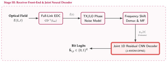
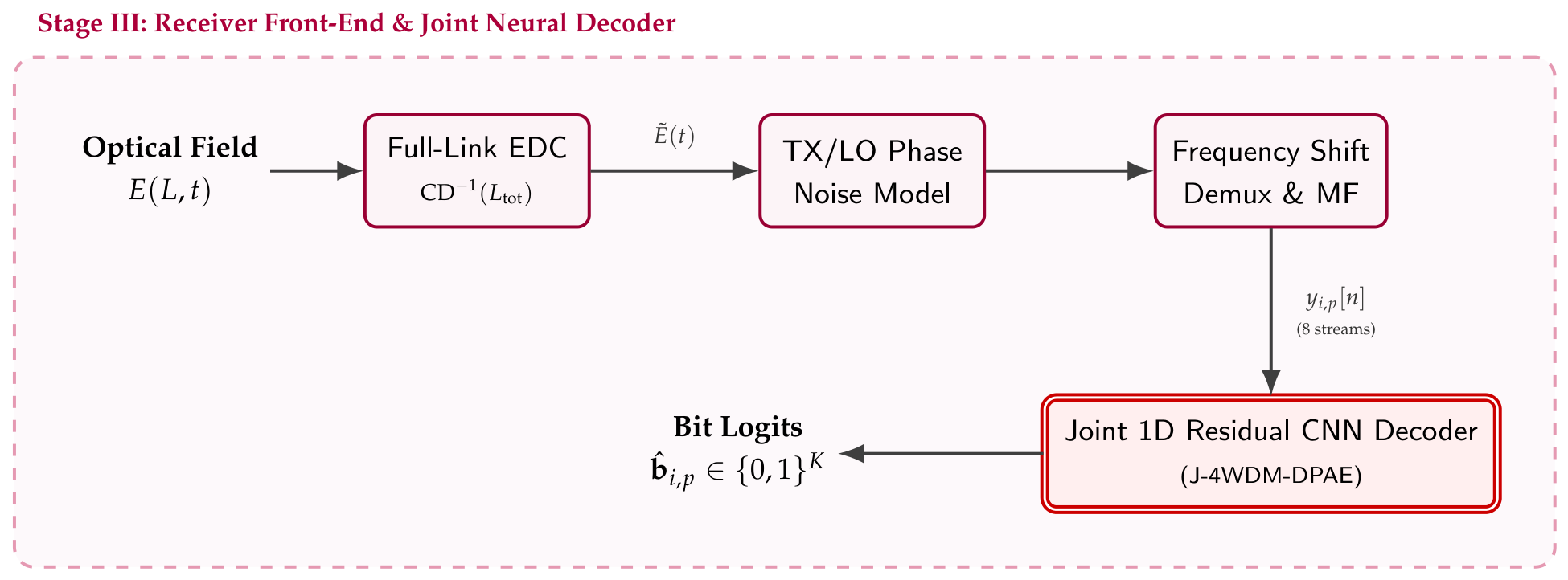
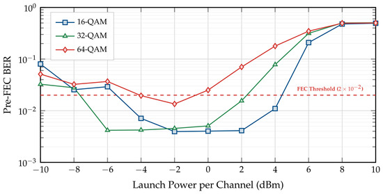
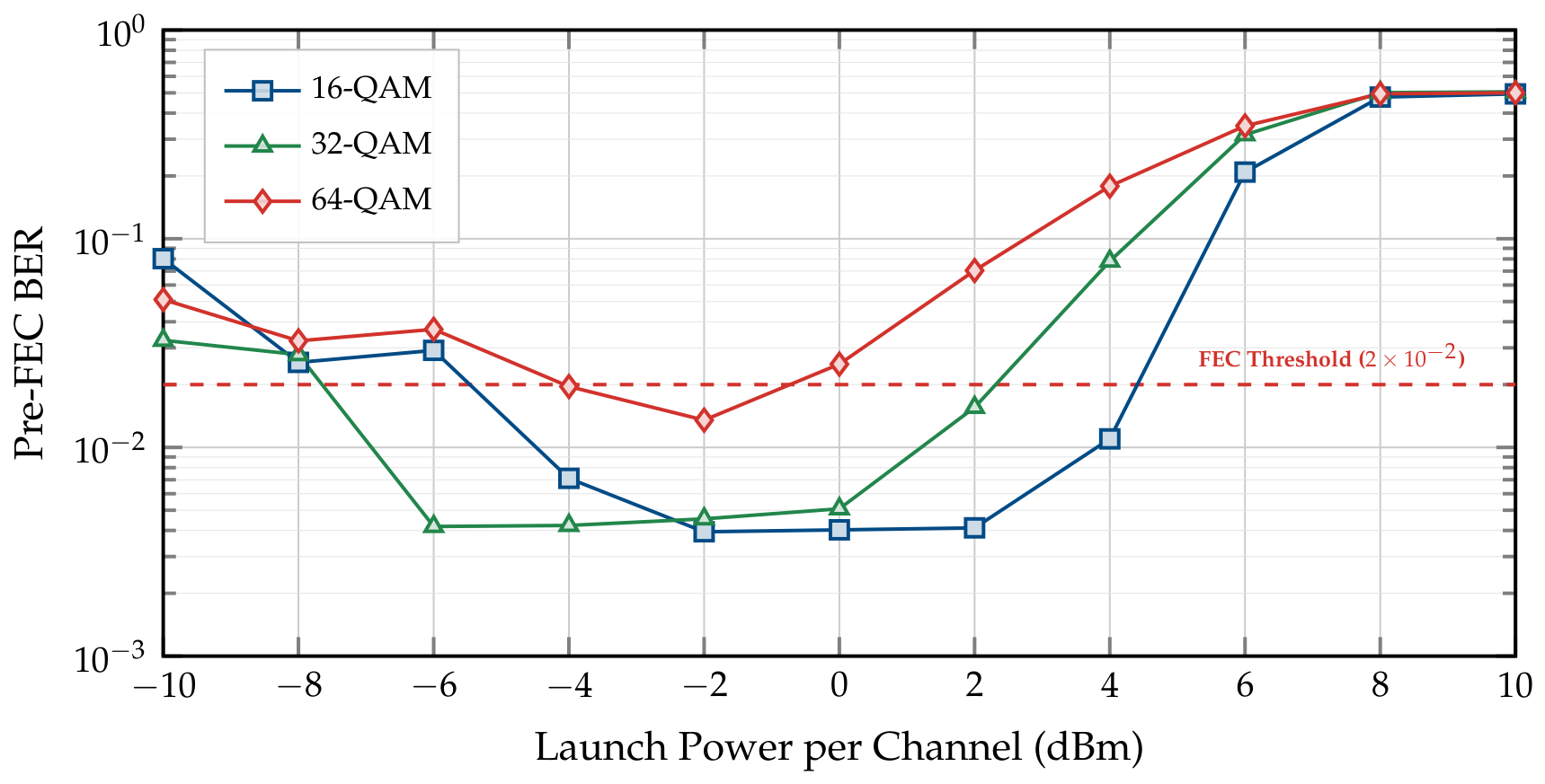
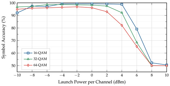
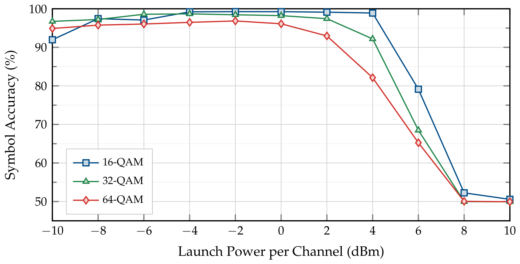
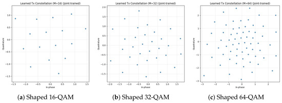
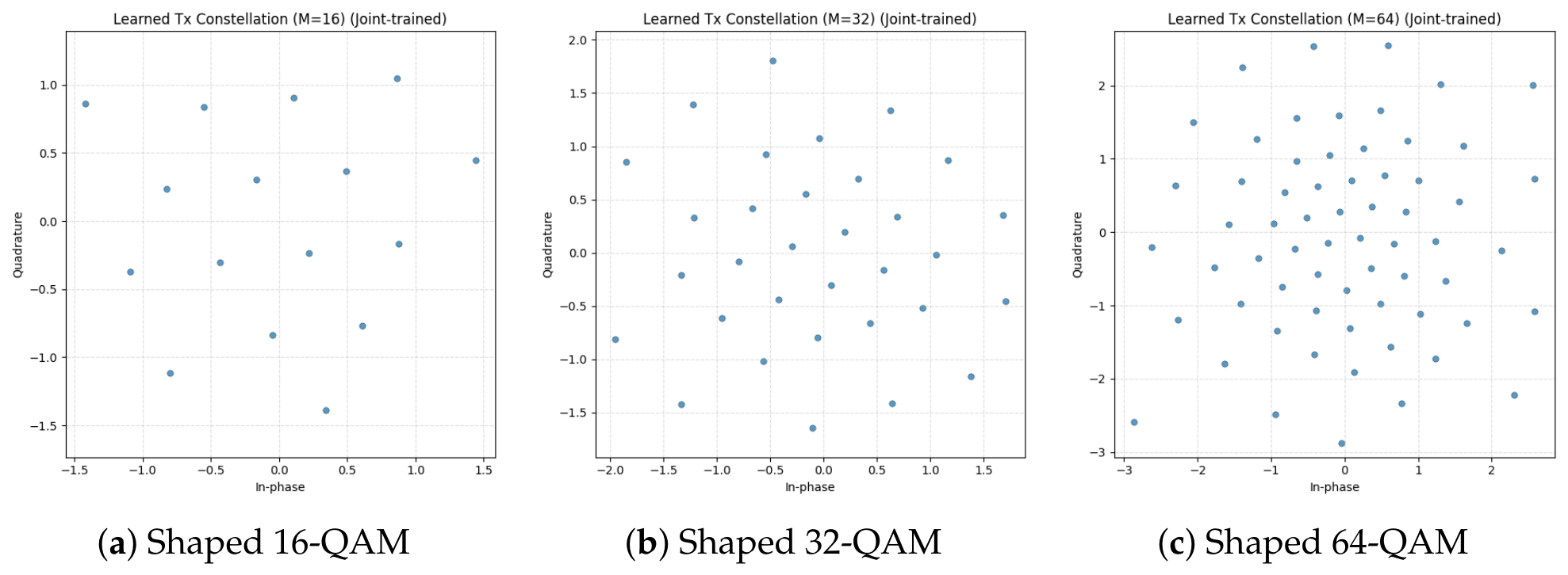
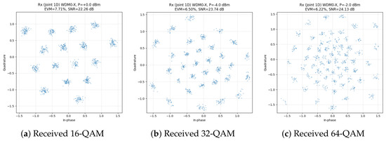
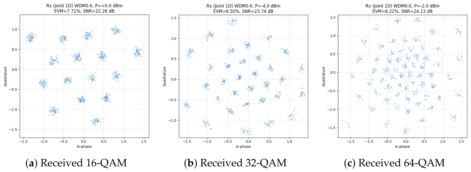
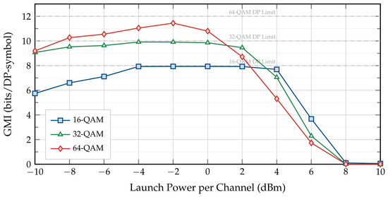
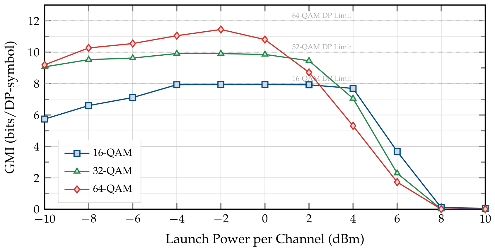
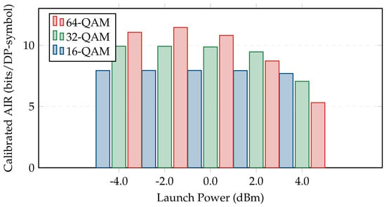
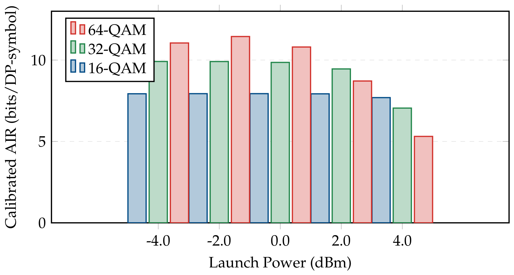
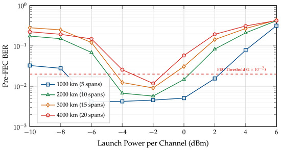
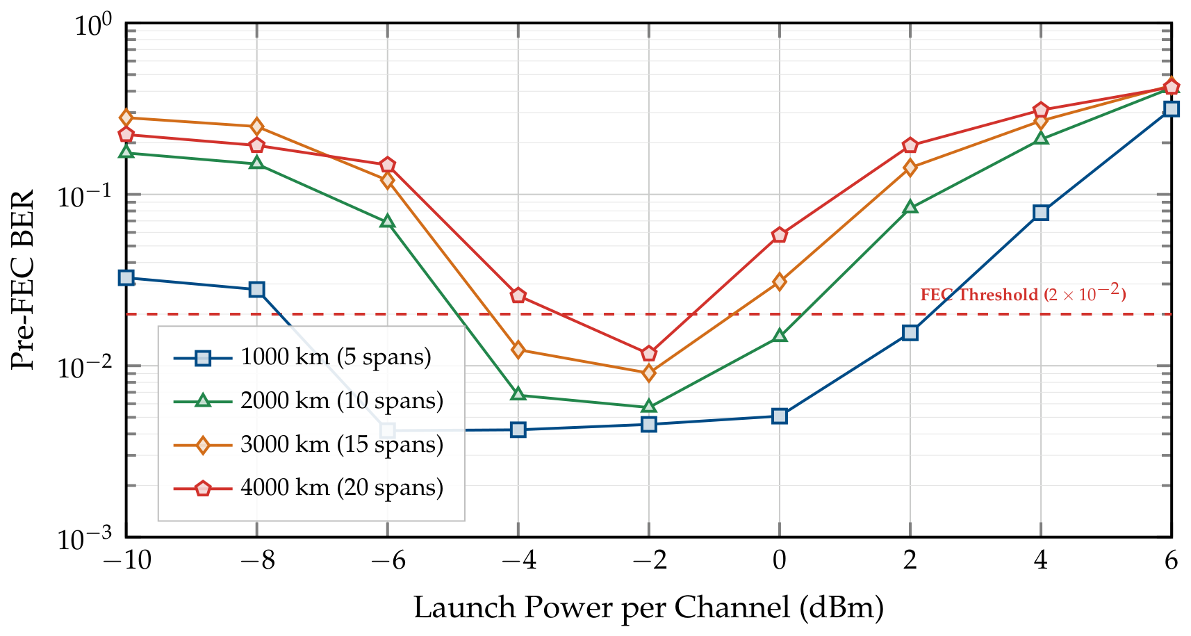
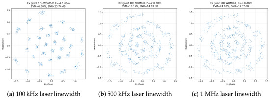
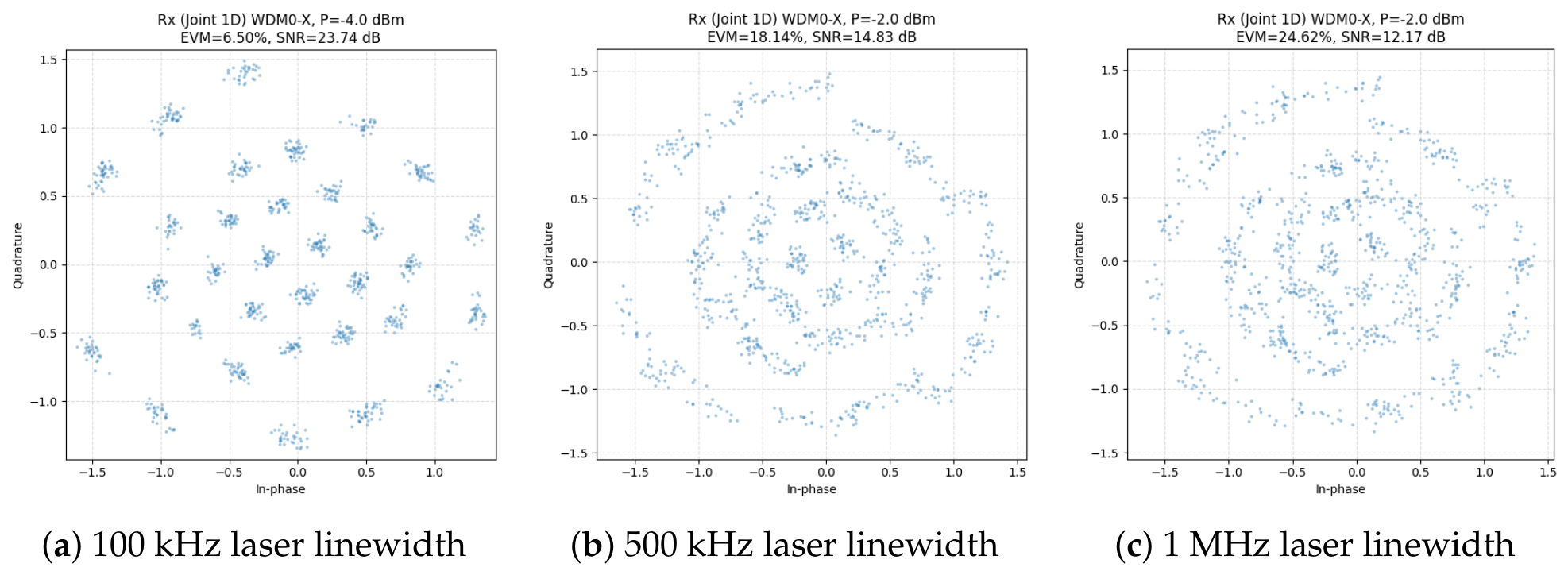
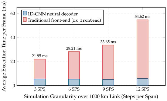
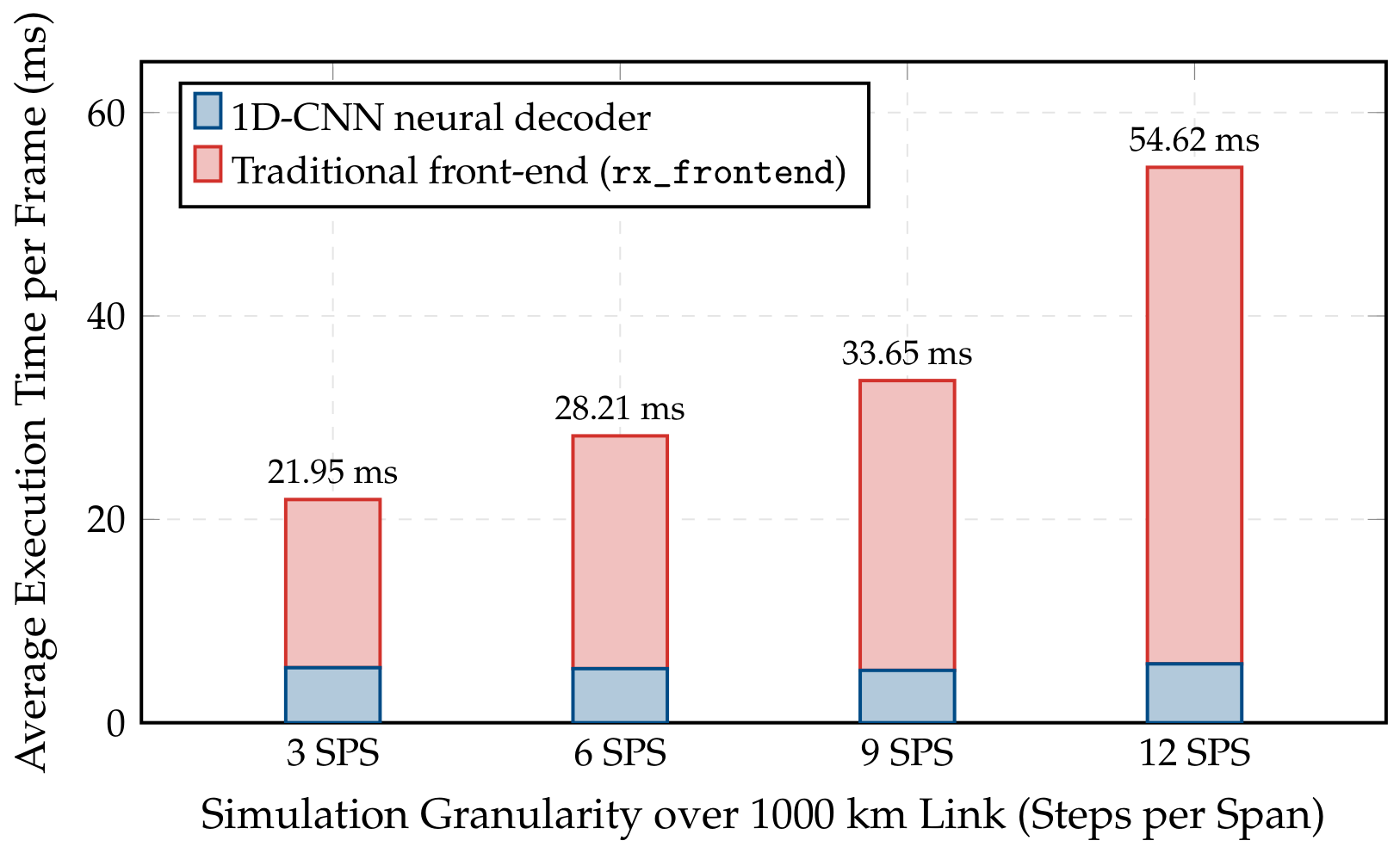

Disclaimer/Publisher’s Note: The statements, opinions and data contained in all publications are solely those of the individual author(s) and contributor(s) and not of MDPI and/or the editor(s). MDPI and/or the editor(s) disclaim responsibility for any injury to people or property resulting from any ideas, methods, instructions or products referred to in the content. |
© 2026 by the authors. Licensee MDPI, Basel, Switzerland. This article is an open access article distributed under the terms and conditions of the Creative Commons Attribution (CC BY) license.