


Abstract
Fringe projection profilometry (FPP) is widely used for high-precision three-dimensional measurement, but its performance is severely degraded when measuring non-Lambertian surfaces with complex reflectance. In such cases, fringe saturation and low modulation lead to unreliable phase values and missing reconstructed data. To address this problem, this paper proposes a photometric feature-guided phase inpainting method for high-dynamic-range FPP. Within the proposed FPP with multi-illumination framework, fringe images are used for phase calculation, while multi-illumination images provide additional photometric cues for phase inpainting. A photometric feature-guided phase inpainting network is designed to extract photometric features from multi-illumination images and fuse them with the damaged phase map. The network is trained on a large-scale synthetic dataset and validated using a prototype system. In standard copper-sphere measurements, PF-PINet increases the average reliable reconstruction ratio from 81.85% to 84.31% while maintaining comparable reconstruction accuracy, indicating that the proposed method can improve measurement completeness for non-Lambertian surfaces.
1. Introduction
Fringe projection profilometry (FPP) has been extensively used as a high-precision optical three-dimensional (3D) measurement technique in industrial inspection, robotic vision guidance, and intelligent manufacturing applications [1]. By projecting structured fringe patterns and establishing a calibrated phase-to-geometry mapping, FPP can provide dense and metric 3D reconstruction with high spatial resolution. However, the measurement of non-Lambertian surfaces with complex reflectance remains a challenging problem. For metallic parts, solder joints, polished components, and other industrial objects, the captured fringe images may suffer from local saturation, low modulation, or severe intensity distortion. These degradations directly affect phase calculation and may lead to unreliable phase values, reconstruction errors, and missing regions in the recovered 3D data [2].
High-dynamic-range (HDR) measurement has therefore become an important research topic in FPP, aiming to extend the effective irradiance range of the imaging system and improve the completeness and accuracy of 3D reconstruction [3]. A representative strategy is multi-exposure fusion. Zhang et al. [4] introduced the multiple-exposure technique into FPP, where fringe patterns captured under different exposure times were combined by selecting unsaturated pixels at each position. Jiang et al. [5] further improved the fusion reliability by selecting the phase value corresponding to the highest fringe modulation. Subsequent studies have focused on exposure optimization and adaptive parameter selection to increase the valid information coverage with limited exposures [6,7,8]. In addition to adjusting camera exposure, the dynamic range can also be extended from the projection side. By exploiting the pixel-level programmability of digital projectors, adaptive projection methods modulate the projected fringe intensity according to scene reflectance, thereby reducing local saturation and improving fringe visibility [9,10,11]. Other methods, including frequency-domain filtering [12] and polarization-based glare suppression [13], have also been investigated for suppressing specular interference. Although these methods are effective in certain scenarios, they still mainly rely on recovering valid fringe information within the conventional camera–projector configuration, and their performance may be limited when the local fringe modulation has been severely degraded.
In recent years, learning-based methods have been introduced into HDR-FPP measurement [14,15]. These methods learn the mapping from degraded fringe or phase data to the desired phase distribution and have shown promising performance in highlight suppression and detail recovery. However, when large phase regions are damaged or missing, a model that only exploits fringe-phase priors may not have sufficient information to infer the correct surface structure. This limitation suggests that, besides improving the fringe images themselves, it is also meaningful to introduce additional observations that are physically related to the measured surface.
The conventional FPP setup has fixed illumination and observation directions determined by the projector and camera. For non-Lambertian surfaces, the reflected intensity is governed by the bidirectional reflectance distribution function (BRDF), which depends on the illumination direction, viewing direction, surface normal, and material reflectance [16]. As a result, the same surface point may exhibit significantly different responses under different illumination directions. Multi-illumination images can therefore provide complementary photometric cues, including shading variation, specular response, local shape-dependent intensity changes, and shadow information. These cues do not directly replace the phase information in FPP, but they can provide additional constraints for damaged phase inpainting when the fringe images are unreliable.
Multi-illumination imaging has been widely used in photometric stereo to estimate surface normals from images captured under different illumination directions [17]. This indicates that multi-illumination images contain rich surface-dependent photometric responses. Existing studies have introduced such photometric information into FPP by using reconstructed surface normals to assist 3D reconstruction or damaged phase recovery [18,19]. These normal-guided methods provide an effective way to incorporate additional geometric constraints into FPP. However, their performance is dependent on the accuracy of the intermediate normal reconstruction, and normal estimation errors may further affect the subsequent reconstruction process.
This paper proposes a photometric feature-guided phase inpainting method for HDR-FPP. Within the proposed FPP with multi-illumination framework, fringe images are used for phase calculation, while multi-illumination images are used to extract photometric features that provide auxiliary cues for damaged phase inpainting. A dedicated phase inpainting network is then designed to fuse the damaged phase map and the extracted photometric features, producing an inpainted phase map for subsequent 3D reconstruction. The network is trained using a large-scale synthetic dataset generated by a physically based rendering engine, and the proposed method is further validated using a developed prototype system.
The main contributions of this work are summarized as follows:
- (1)
- A photometric feature-guided phase inpainting strategy is proposed for HDR-FPP measurement of non-Lambertian surfaces, in which multi-illumination images provide complementary photometric cues for recovering unreliable phase regions.
- (2)
- PF-PINet is developed to directly extract illumination-dependent photometric features from multi-illumination images and integrate them with phase-domain information through a coarse-to-fine phase inpainting framework.
- (3)
- A physically based synthetic data-generation pipeline is developed for network training and evaluation, and a prototype FPP system with multi-illumination imaging is developed for experimental validation. Experiments on synthetic and real data are conducted to verify the effectiveness of the proposed method.
2. Principle and Problem Formulation
2.1. Radiometric Analysis of Reflection
Under ideal conditions, the irradiance–reflection relationship in an imaging system [20] can be expressed as
where I denotes the reflected radiance captured by the camera sensor, and is an intensity coefficient determined by the system response coefficient , the exposure time t, and the incident irradiance . The unit vectors and denote the illumination and viewing directions, respectively, while is the surface normal at the measured position. The function characterizes the surface reflectance property. For an ideal Lambertian surface, the BRDF reduces to a constant , determined by the diffuse reflectance coefficient , and is independent of illumination or viewing direction. In contrast, non-Lambertian surfaces exhibit nonlinear dependencies on and , leading to complex directional reflectance behavior [16].
To analyze the influence of directional reflectance, a spherical coordinate system is established with the camera optical axis aligned along Z and the viewing direction fixed at . The surface normal and illumination zenith angle are kept constant, while the illumination azimuth angle and the intensity coefficient are varied to examine the changes in captured radiance.
Figure 1 shows the polar distribution of captured radiance for an approximately Lambertian matte ceramic surface and a non-Lambertian alumina surface with a roughness coefficient of 0.2. For the Lambertian surface, the radiance variation is mainly determined by the cosine term and the intensity coefficient , so adjusting exposure time or incident intensity can usually bring the captured signal into the valid dynamic range. In contrast, the non-Lambertian surface exhibits a much stronger directional dependence. Under certain illumination directions, the captured radiance may still fall outside the valid dynamic response range even when the intensity coefficient is adjusted. This indicates that, under non-Lambertian reflection, HDR strategies based only on intensity adjustment may be insufficient when directional reflectance dominates the fringe degradation.
Figure 1.
Polar distribution of captured radiance for an approximately Lambertian matte ceramic surface and a non-Lambertian alumina surface with a roughness coefficient of 0.2.
2.2. Multi-Illumination Cues and Photometric Feature Representation
The directional dependence of non-Lambertian reflection motivates the use of the FPP with multi-illumination framework proposed in this work, as illustrated in Figure 2. In this framework, fringe images are used for phase calculation, while multi-illumination images provide additional observations of the same surface under different illumination directions.
Figure 2.
Schematic of the FPP with multi-illumination framework. Fringe images are used for phase calculation, while multi-illumination images provide additional photometric observations under different illumination directions.
Figure 3 illustrates the complementary relationship between these two types of images at the information level. For a non-Lambertian hemispherical object, Figure 3a,b show fringe images under two different projection intensities. Due to the directional reflectance of the surface, changing the projection intensity cannot completely eliminate unreliable regions caused by specular reflection. Figure 3c,d show images captured under two different illumination directions. Although the multi-illumination images do not provide structured phase encoding, they contain complementary surface-dependent intensity cues related to local shape, shading, and reflectance variations, especially in regions where the fringe images are locally unreliable.
Figure 3.
Complementary information provided by fringe projection and multi-illumination imaging on a non-Lambertian hemisphere. (a,b) Fringe images under two different projection intensities. (c,d) Images captured under two different illumination directions.
Such multi-illumination observations have been widely studied in photometric stereo for surface normal estimation. Classical photometric stereo estimates the surface normal from images captured under multiple illumination directions under the Lambertian assumption [21]. Given the illumination direction matrix and the captured radiance vector , the surface normal can be estimated as
where denotes the pseudo-inverse of . Although this classical model is sensitive to non-Lambertian reflectance, recent data-driven photometric stereo methods have shown that multi-illumination images can still be used to estimate surface normals for non-Lambertian surfaces by learning from large-scale data [22,23,24].
Based on this observation, our previous work [19] attempted to use normals reconstructed by a data-driven photometric stereo method to guide FPP phase inpainting. This method improved the reconstruction of non-Lambertian surfaces to some extent, but its performance depended on the accuracy of the intermediate normal reconstruction. When the estimated normals were inaccurate, the errors could be propagated to the subsequent phase inpainting process.
In data-driven photometric stereo, surface normals are not obtained directly from raw image intensities. Instead, multi-illumination observations are first transformed into high-dimensional feature representations, which are then decoded or regressed into three-channel normal maps. Although different methods construct these representations in different forms, they share a similar principle. For example, CNN-PS organizes pixel-wise multi-illumination observations into observation maps for normal regression [22], while PS-FCN extracts features from images captured under different illumination directions and aggregates them for normal estimation [23]. These methods suggest that the normal map is a compact geometric representation derived from richer photometric features related to surface shape, shading, shadowing, and reflectance variations. Therefore, instead of using reconstructed normals as intermediate constraints, this work directly introduces photometric features extracted from multi-illumination images into the FPP measurement pipeline. This allows phase-domain processing to exploit photometric information beyond the compact normal representation while avoiding potential error propagation caused by normal reconstruction.
2.3. Photometric Feature-Guided Phase Inpainting Formulation
In a standalone FPP measurement pipeline, the unwrapped phase is first decoded from the captured fringe images using a phase-shifting algorithm [25]:
where denotes the intensity of the i-th fringe image, T is the fringe order obtained from the phase-unwrapping process, is the number of phase-shifting steps, and is the phase shift.
After obtaining , the 3D coordinates of each pixel are computed from the calibrated system model [26]:
where , , and are calibration coefficients along the X, Y, and Z axes, respectively. These coefficients are determined through system calibration and remain fixed during measurement.
Equations (3) and (4) show that the phase map is the core intermediate variable in FPP. When fringe saturation or low modulation occurs, phase errors are introduced during phase decoding and are further propagated to the reconstructed 3D coordinates. Therefore, this work formulates HDR measurement of non-Lambertian surfaces as a photometric feature-guided phase inpainting problem. Given a damaged phase map and a set of multi-illumination images , the phase inpainting process is expressed as
where denotes the damaged phase map, is the inpainted phase map, and denotes the set of multi-illumination images. Here, H and W denote the image height and width, respectively, and represents the photometric feature-guided phase inpainting function.
The function is expected to exploit both the damaged phase map and the photometric features extracted from multi-illumination images. The valid regions in provide the geometric baseline and structural continuity of the measured surface, while the photometric features provide complementary information for inferring phase values in unreliable regions. Therefore, can be regarded as a phase-domain inpainting function guided by multi-illumination photometric features.
Based on this formulation, the inpainting process is performed in the phase domain rather than in the reconstructed point-cloud domain. Since phase errors caused by saturation or low modulation are propagated to the 3D coordinates through Equation (4), correcting the damaged phase before 3D reconstruction addresses the measurement error closer to its source. Meanwhile, the phase map retains a regular image structure and is pixel-wise aligned with the captured multi-illumination images, which facilitates image-domain feature fusion. After inpainting, remains a standard phase map and can be converted into 3D coordinates using the original calibrated phase-to-geometry mapping. Thus, the proposed formulation introduces photometric cues into FPP without changing the calibrated geometric model of the system.
3. Proposed Method
The phase inpainting function involves complex nonlinear relationships among non-Lambertian reflectance, phase degradation, and multi-illumination photometric observations, making it difficult to explicitly describe with parametric models. Leveraging the feature extraction and nonlinear approximation capabilities of deep neural networks, this work models in a data-driven manner. Specifically, a Photometric Feature-Guided Phase Inpainting Network (PF-PINet) is proposed to learn this mapping by extracting photometric features from multi-illumination observations and integrating them with phase-domain information for damaged phase inpainting.
3.1. Network Architecture
The overall pipeline of the proposed PF-PINet is illustrated in Figure 4a, which consists of five main components as follows.
Figure 4.
Illustration of the proposed PF-PINet: (a) overall pipeline of PF-PINet; (b) UNet++-based multi-scale feature fusion module.
Shared-weight photometric feature extractor. Inspired by the shared-weight feature extraction and max-pooling fusion scheme in PS-FCN [23], this module is designed to extract and aggregate photometric features from images captured under different illumination directions. For each illumination source, its 3D direction vector is spatially expanded into a three-channel direction map and concatenated with the corresponding input image along the channel dimension, forming a 6-channel tensor as input. All illumination conditions are independently processed by the same fully convolutional backbone with shared weights. Since the network parameters are shared across illumination observations, the feature extraction process is structurally decoupled from the number of input illumination sources, and the same backbone can be applied to an arbitrary number N of illumination inputs without modifying the network architecture.
The photometric features extracted under different illuminations are then fused by max pooling along the illumination dimension:
where c denotes the channel index, are spatial coordinates, and denotes the feature map associated with the i-th illumination. This max-pooling operation provides a simple parameter-free and permutation-invariant aggregation of the illumination set. In particular, changing N affects only the number of feature maps participating in the pooling operation, while the dimensionality of the aggregated feature remains unchanged. Therefore, the photometric encoding does not require a fixed number or ordering of illumination observations.
The fused photometric feature forms a dense 128-channel feature tensor, where each spatial location is represented by an illumination-aggregated photometric feature vector. This tensor representation is preserved and subsequently aligned with the phase feature for cross-modal feature fusion, allowing the network to exploit complementary photometric information from multiple illumination observations directly in the feature space.
Phase feature extractor. In the phase inpainting task, the undamaged regions of the phase map provide reliable geometric references and boundary constraints, while the damaged regions require reconstruction by the network. Since phase maps exhibit typical image structural properties, the phase feature extractor takes the damaged phase as input and progressively extracts deep structural representations through a series of convolutional layers. The resulting phase feature encodes both local geometric details and global phase continuity, supplying a stable geometric prior that complements photometric features and supports subsequent cross-modal fusion.
UNet++-based multi-scale feature fusion module. The multi-scale feature fusion module is designed to deeply integrate photometric and phase features, as illustrated in Figure 4b. The photometric features are first upsampled via transposed convolution to match the spatial resolution of the phase features. The two modalities are then concatenated along the channel dimension and passed through a convolution to compress channels and generate an initially aligned cross-modal representation. This fused representation is further processed by a three-level UNet++ architecture [27], which leverages dense skip connections, cross-scale interactions, and nested decoders to progressively integrate multi-scale semantics and refine geometric details. The resulting fused feature serves as the input to both the coarse inpainting and refinement modules.
Mask-guided coarse inpainting module. The coarse inpainting module performs an initial reconstruction of the phase map using the fused feature . After passing through several convolutional layers with progressive dimensionality reduction, the network outputs a preliminary reconstruction .
Since the coarse inpainting stage predicts a complete phase map, directly replacing all pixels with would introduce unnecessary deviations in regions where the original phase values are already reliable. Therefore, the reconstruction should be applied only to recoverable damaged regions. In HDR-FPP measurement, such regions should satisfy two conditions: the phase is unreliable due to low fringe modulation, and the corresponding pixel still belongs to the observable region of the FPP system. Pixels caused by occlusion or outside the valid observable region do not have valid phase correspondence and should be excluded from phase inpainting.
To this end, a mask-gated strategy is adopted by introducing a binary damaged-region mask . The coarse phase is obtained by enforcing only in the selected damaged regions while preserving the original phase elsewhere:
where ⊙ denotes element-wise Hadamard multiplication.
The phase reliability is evaluated using the fringe modulation map computed from the phase-shifting sequence:
A high modulation value indicates reliable phase decoding, whereas a low modulation value usually corresponds to unreliable phase values caused by saturation or insufficient exposure.
In addition to phase reliability, the observability of each pixel is estimated using the average intensity of the phase-shifting sequence:
The average intensity represents the DC component of the captured fringe sequence. A very low value of indicates that the corresponding pixel receives insufficient effective irradiance from the projected fringes, which usually occurs in occluded regions or outside the valid observable region of the FPP system. Such pixels are not considered recoverable by phase inpainting.
The final binary mask is defined by jointly considering the modulation map and the average intensity:
where and are predefined thresholds for modulation and average intensity, respectively.
This mask-gated mechanism restricts coarse inpainting to low-modulation but observable regions. It preserves reliable phase values in intact regions and excludes physically invalid pixels from the inpainting process, thereby providing a more appropriate initialization for subsequent refinement.
Complex-domain residual refinement module. To further enhance the phase accuracy, the refinement module adopts a residual learning strategy that improves the coarse phase by directly predicting its residual components. Since phase values are highly sensitive to noise, performing residual regression directly in the real domain can lead to unstable predictions. To obtain a noise-robust and continuous representation, the coarse phase is first mapped into the complex domain through Euler’s formula:
where denotes the two-channel complex-valued encoding. The unit-magnitude constraint of this representation provides a smoother and more stable feature space for residual estimation while suppressing noise-driven fluctuations.
The complex-domain phase is concatenated with the scale-aligned fused feature along the channel dimension and fed into a convolutional network, which learns to predict the complex-domain residual . The predicted residual is then mapped back to the real domain using the inverse tangent:
where and denote the real and imaginary components, respectively.
Finally, the network outputs the inpainted phase by adding the real-domain residual to the coarse phase:
Overall, PF-PINet organizes phase inpainting according to the complementary roles of photometric observations and phase-domain information. Multi-illumination observations are used to introduce surface-dependent photometric information into regions where the fringe-derived phase is unreliable, whereas the phase representation provides the geometric context required for phase-domain reconstruction. Their joint representation is used for selective reconstruction of recoverable damaged regions, followed by residual refinement of the reconstructed phase, while reliable phase measurements are retained by the mask-gated formulation. The overall architecture therefore combines photometric feature guidance, selective phase reconstruction, and residual refinement within a unified phase-domain framework.
3.2. Loss Functions
According to the distinct mechanisms of the coarse inpainting and residual refinement modules in PF-PINet, separate supervision terms are designed for the coarse phase , the final output , and the complex-domain residual , enabling stage-wise optimization tailored to each module.
For real-domain phase supervision, the phase loss is composed of a pixel-wise loss , a structural similarity loss , and a gradient consistency loss :
where and are weighting factors for the structural similarity and gradient consistency terms, respectively.
The pixel-wise loss provides direct numerical supervision for the predicted phase map. For a predicted phase map and the ground-truth phase map , it is defined using the Huber loss:
where denotes the Huber loss:
Compared with the standard squared error, the Huber loss improves robustness to local outliers while maintaining accurate numerical supervision.
The structural similarity loss is introduced to preserve local structural consistency in the phase map:
where is computed following [28]. This term encourages the predicted phase to maintain local structural similarity with the ground truth, rather than only minimizing point-wise errors.
The gradient consistency loss is designed according to the local monotonic and continuous variation of the unwrapped phase along the principal coding direction of FPP. In the adopted phase representation, this direction corresponds to the horizontal direction. Therefore, the gradient loss is defined as
where denotes the finite difference along the horizontal direction. In the adopted FPP configuration, the camera and projector are arranged with approximately parallel optical axes, while the camera–projector baseline and fringe coding direction are predominantly aligned with the image horizontal axis. Therefore, the principal phase variation associated with depth changes occurs along the x direction, and the horizontal gradient is used to constrain local phase continuity.
Overall, is formulated with the pixel-wise Huber loss as the primary numerical supervision, while the SSIM and gradient terms provide complementary constraints on local structural similarity and phase-gradient continuity. In this way, the loss function balances point-wise phase accuracy with local structural preservation during phase reconstruction. The weighting factors and control the relative contributions of the two auxiliary terms and are empirically selected according to the training objective.
For the refinement module, supervision is further applied to the complex-domain residual. The ground-truth residual is constructed as the complex phase difference between the ground-truth phase and the coarse phase:
Residual learning is then performed by minimizing the Euclidean distance between the predicted complex-domain residual and the ground-truth residual:
This complex-domain supervision provides a bounded representation for residual refinement and improves the stability of local phase correction.
3.3. Training Strategy
A progressive three-stage training strategy is adopted to match the coarse-to-fine architecture of PF-PINet and reduce optimization interference between the coarse inpainting and residual refinement modules.
Stage 1: Coarse inpainting training. In the initial stage, the parameters of the residual refinement module are frozen, while the photometric feature extractor, phase feature extractor, multi-scale feature fusion module, and mask-guided coarse inpainting module remain trainable. The coarse phase is supervised by the real-domain phase loss . Since includes pixel-wise, structural, and gradient consistency terms, this stage enables the network to learn a stable coarse reconstruction while preserving the structural continuity of the phase map. A relatively larger is used at this stage to place greater emphasis on the recovery of the overall phase structure during coarse reconstruction.
Stage 2: Residual refinement training. After the coarse inpainting module has converged, all modules except the residual refinement module are frozen. The refinement module is trained independently using the complex-domain residual loss , which directly supervises the predicted residual . This stage allows the refinement branch to focus on learning residual corrections in the complex representation without interfering with the coarse inpainting capability established in Stage 1.
Stage 3: Joint fine-tuning. Finally, all network parameters are unfrozen and jointly fine-tuned with a reduced learning rate. In this stage, the final output phase is supervised by the real-domain phase loss . The lower learning rate helps preserve the coarse reconstruction and residual refinement abilities learned in the previous stages, while allowing different modules to adapt to each other during end-to-end optimization. Meanwhile, is reduced to emphasize fine numerical correction of the final phase output.
This staged training process first establishes a reliable coarse phase initialization, then learns local residual correction, and finally improves the consistency between different modules through joint fine-tuning. It provides a stable optimization procedure for the proposed coarse-to-fine phase inpainting network.
4. Experiments
Since training PF-PINet requires large-scale data and obtaining ground-truth phase for real objects is challenging, a dedicated synthetic dataset is generated for network training and synthetic evaluation. In addition, a prototype system based on the FPP with multi-illumination framework is developed to collect real-world data and validate the measurement accuracy and practical effectiveness of the proposed method.
4.1. Synthetic Dataset and Training
4.1.1. Dataset Generation
The dataset generation pipeline is implemented using the physically based rendering engine Mitsuba [29] to simulate the full working process of the FPP with multi-illumination imaging system. The implementation details are described as follows.
Imaging system simulation. By extending Mitsuba through plugin customization, we constructed a simulated imaging system that follows the same principles as the prototype FPP with multi-illumination system and consists of three major components:
Camera. A perspective-sensor plugin with a resolution of is employed. The field of view (FOV) is randomly selected within 18–, and the sensor coordinate system is used as the reference frame for the entire rendering space.
Illumination. Thirty directional-emitter plugins are randomly distributed over the upper hemisphere with respect to the camera optical axis. Their intensities follow Mitsuba’s default emission model, allowing physically based simulation of shading and BRDF interactions under different illumination directions.
Fringe projector. A four-step phase-shifting fringe pattern set with 64 fringe periods is loaded onto a custom perspective-emitter plugin to simulate the fringe projector. The projector’s FOV is randomized within 20–, with its optical axis constrained to lie in the same horizontal plane as the camera. The angle between the projector and camera optical axes is randomly set to 20–, and the output intensity is scaled to – times the default illumination level.
Object property configuration. To simulate real-world reflectance behavior during measurement, a series of 3D digital models are collected and configured in terms of shape, material, and spatial pose to construct a diverse object library.
Shape. A total of 50 shape models are used, including 40 models from the Blobby and Sculpture datasets of [30], where the Blobby shapes exhibit smooth, low-frequency surface features and the Sculpture shapes contain sharp, high-frequency geometric details. The remaining 10 models are industrial part geometries collected from authorized online sources to improve applicability in industrial scenarios.
Material. Material properties are defined using 62 measured isotropic BRDFs from the MERL BRDF database [31]. This dataset contains physically measured reflectance profiles of real-world materials captured under controlled laboratory conditions, enabling the rendering process to reproduce diverse reflectance behaviors such as diffuse reflection and mixed diffuse–specular interactions commonly observed on metallic and non-Lambertian surfaces.
Spatial. Each model is initially placed 500 mm in front of the camera, then scaled by a random factor between 0.5 and 1.5 and subjected to a random 3D rotation, emulating practical variations in object placement.
Rendering configuration and sample generation. All scenes are rendered using Mitsuba’s physically based path-tracing integrator. The rendering process uses 256 samples per pixel to obtain stable radiance estimation and simulate light transport under multi-illumination conditions, particularly for specular highlights and complex BRDF interactions.
For each object instance, a randomized FPP with multi-illumination imaging configuration is instantiated within the predefined parameter ranges. The system renders a set of fringe patterns and multi-illumination images. The damaged phase map is obtained by applying the phase-decoding algorithm in Equation (3) to the rendered fringe patterns, while the corresponding ground-truth phase map is extracted using Mitsuba’s inverse ray-tracing functionality. Each generated sample therefore contains 10 fringe images, including 4 phase-shifting images and 6 Gray-code images, 30 directional-light illumination images, a damaged phase map, and its corresponding ground-truth phase map.
Following this procedure, the synthetic dataset is constructed by pairing each of the 50 shape models with 6 randomly selected BRDF materials and rendering them under 100 randomized spatial configurations, resulting in a total of 30,000 samples. Representative examples are shown in Figure 5. By reproducing the optical behavior of the FPP with multi-illumination system, the dataset covers variations in geometry, material, illumination, and projection conditions, providing a diverse basis for network training.
Figure 5.
Examples of the synthetic dataset. (a) Fringe rendering of a non-Lambertian material; (b) Fringe rendering of a Lambertian material; (c,d) Multi-illumination images of a non-Lambertian material under different illumination directions; (e) Ground-truth phase map; (f) Phase error map between the damaged and ground-truth phases.
4.1.2. Training Configuration
The 30,000-sample synthetic dataset is divided at a 9:1 ratio, with 90% of the samples used for network training and the remaining 10% reserved only for internal performance monitoring during training. Samples in the latter subset are not used for network parameter optimization or for the final quantitative evaluation. Before being fed into the network, each sample undergoes the following preprocessing steps:
Normalization: Based on the 64-period structure of the phase map, the raw phase values (0–128) are linearly normalized from the range [0, 128] to [0, 1]. Similarly, the multi-illumination images are linearly normalized from their original intensity range [0, 255] to [0, 1].
Cropping and Rescaling: For each sample, all input tensors, including illumination images and phase maps, are processed using one of the following two strategies: (1) center cropping to a resolution of ; (2) cropping based on the shorter side followed by resizing to .
It should be noted that the cropping operation is only used during the training stage. This design is adopted to increase training data diversity and to reduce GPU memory consumption as well as training time. During inference, the full-resolution experimental images are directly used as network inputs without resizing or cropping, and the output phase map is generated at the same resolution as the input images.
Image Sampling: For each sample, 30 images rendered under different illumination directions form a candidate illumination set. During training, 10–20 illumination images are randomly selected from this set for each batch as network inputs. This random sampling strategy exposes the network to varying illumination counts during training and, together with the shared-weight feature extractor and max-pooling aggregation, reduces the dependence of the learned representation on a fixed number of input illumination sources.
The training framework is implemented using PyTorch (version 2.5.0) [32]. The network contains approximately 5.2 million learnable parameters. Following the multi-stage training strategy described in Section 3.3, the full training procedure is performed on a workstation equipped with an NVIDIA RTX 4090D GPU. A total of 50 epochs are used for training, and the overall runtime is approximately 12 h.
The mask thresholds are selected empirically according to their roles in the staged training process. The modulation threshold controls the extent of low-modulation regions involved in phase reconstruction. A relatively larger threshold is used during coarse-stage training to expose the network to broader damaged regions and strengthen its ability to reconstruct severe phase degradation. In the subsequent stages, a stricter threshold is adopted because moderately degraded regions can retain partially usable phase information and are further corrected by residual refinement. The average-intensity threshold is mainly used to exclude occluded or unobservable regions and is therefore kept fixed throughout training. The main training hyperparameters are summarized in Table 1.
Table 1.
Training hyperparameters for the three-stage optimization. Stage 1 performs coarse inpainting, Stage 2 performs residual refinement, and Stage 3 performs joint fine-tuning.
4.2. Evaluation on Synthetic Data
The proposed PF-PINet is evaluated on an additional synthetic validation set containing 150 samples generated separately after network training using the same rendering pipeline. These samples are not used for network training, parameter optimization, or internal performance monitoring. Each sample is independently generated with randomized object pose, position, scale, and illumination conditions, while the material configurations are selected from several BRDFs with pronounced non-Lambertian reflectance to emphasize challenging HDR measurement conditions. Although the validation set is not explicitly constructed as a strict shape-disjoint benchmark, the independently generated configurations produce different phase distributions and photometric observations from those used during training, and all compared methods are evaluated on exactly the same samples and measurement conditions. To provide inputs for the traditional multi-intensity HDR baseline, three sets of fringe images are generated for each sample using projection intensities scaled by factors of 0.5, 1, and 2.
The evaluation considers phase accuracy, root mean square error (RMSE), and signal-to-noise ratio (SNR). For a predicted phase map and the ground-truth phase map , the RMSE is calculated as
and the SNR is defined as
where RMSE is reported in radians and SNR in decibels (dB).
Although RMSE and SNR provide global measures of the phase reconstruction error, severely damaged phase regions in HDR-FPP may contain large invalid errors that dominate these metrics and weaken the distinction between usable and unusable phase estimates. Therefore, phase accuracy is additionally introduced to evaluate the proportion and quality of usable phase reconstruction. It is defined as
where
The two thresholds in Equation (24) are selected according to different considerations. The lower threshold of 0.1 rad is used as a practical tolerance to distinguish small phase perturbations from the more pronounced degradation considered in HDR-FPP. The upper threshold of rad has a more direct physical and algorithmic interpretation in FPP phase reconstruction: errors exceeding rad generally indicate severe phase mismatch, such as an incorrect fringe order or phase-unwrapping failure. In addition, the residual refinement branch of PF-PINet predicts phase corrections within . Therefore, errors larger than rad are treated as unsuccessful recovery and assigned zero score, while intermediate errors are linearly weighted. This definition therefore provides a bounded evaluation of phase usability and avoids excessive influence from invalid large-amplitude phase errors.
The compared methods include the initial damaged phase, two baseline methods, and four ablation variants. The initial damaged phase is reported as the input reference. The baseline methods include the traditional multi-intensity HDR method based on intensity fusion [5] and the previous normal-guided phase inpainting method [19]. The four ablation variants evaluate the effects of photometric guidance, the mask-gated mechanism, the complex-domain residual representation, and the staged training strategy, respectively. Specifically, the corresponding variants remove the photometric guidance, remove the mask-gated mechanism, replace the complex-domain residual with direct real-domain residual regression, and replace the proposed staged optimization with end-to-end training. All ablation variants are evaluated using the same synthetic dataset and evaluation protocol as the full PF-PINet, with only the design factor under investigation modified in each experiment.
Table 2 summarizes the quantitative results of all compared methods on the synthetic validation set. In addition to the overall phase accuracy, SNR, and RMSE, the phase accuracy is further evaluated in the severely damaged regions to specifically assess phase inpainting performance in these regions. These regions are defined from the initial damaged phase as pixels whose absolute phase error with respect to the ground truth exceeds rad, and the same fixed region is used for all compared methods. Figure 6 presents representative phase residual maps for the baseline methods and the two structural ablations involving photometric guidance and mask gating.
Table 2.
Quantitative evaluation of phase inpainting performance on the synthetic validation set.
Figure 6.
Visual comparison of phase inpainting results on the synthetic data. (a) Ground-truth phase; (b) residual of the initial damaged phase; (c) residual of the phase reconstructed by the traditional HDR method; (d) residual of the phase inpainted by the normal-guided method; (e) residual of the phase inpainted by the ablation model without photometric guidance; (f) residual of the phase inpainted by the ablation model without the mask-gated mechanism; (g) residual of the phase inpainted by the proposed PF-PINet.
4.2.1. Comparison with Baseline Methods
As shown in Table 2, the proposed PF-PINet achieves the best performance among the compared methods in terms of phase accuracy, RMSE, and SNR. Compared with the initial damaged phase, PF-PINet increases the phase accuracy from 84.94% to 97.19%, while reducing the RMSE from 52.73 to 1.13. These results demonstrate that the proposed photometric feature-guided strategy can effectively recover usable phase information from severely degraded non-Lambertian samples.
The traditional multi-intensity HDR method improves the phase accuracy to 89.30%, indicating that projection-intensity modulation can partially reduce phase degradation caused by overexposure or insufficient exposure. However, its RMSE remains high, and the residual map in Figure 6c shows that obvious phase errors remain after HDR fusion. This behavior is consistent with the radiometric analysis in Section 2.1. Varying the projection intensity changes the irradiance level but does not alter the projection–observation geometry. Therefore, for non-Lambertian surfaces with strong directional reflectance, some regions may remain poorly modulated under all tested projection intensities. As a result, multi-intensity fusion can recover part of the exposure-related phase degradation but cannot fully resolve phase loss associated with directional reflectance. In contrast, PF-PINet introduces multi-illumination images acquired under different illumination directions as auxiliary photometric observations, providing additional surface-dependent cues for inferring phase values in regions where the fringe-derived phase is unreliable.
The normal-guided phase inpainting method achieves higher phase accuracy than the traditional HDR method, confirming that auxiliary geometric information is beneficial for phase-domain repair. However, its accuracy is still lower than that of PF-PINet. Although both methods perform inpainting in the phase domain, the normal-guided method first reconstructs surface normals using PS-FCN and then feeds the estimated normal map into the phase inpainting network. This two-step strategy may propagate normal estimation errors to the subsequent phase repair stage. Moreover, the normal map is a compact three-channel representation, which may discard part of the illumination-dependent information contained in the original multi-illumination observations. In contrast, PF-PINet directly extracts photometric features from multi-illumination images, preserving richer cues related to shading, shadowing, and reflectance variations for phase inpainting.
This direct photometric feature-guided design also improves computational efficiency. The average inference time is measured on an NVIDIA RTX 4090D platform with an input resolution of , 15 multi-illumination images, and 32-bit floating-point inference. The PS-FCN + normal-guided baseline requires 67.53 ms per sample with a peak allocated GPU memory of 1739 MB, whereas PF-PINet requires 45.11 ms per sample with a peak allocated GPU memory of 1694 MB, reducing the inference time by approximately 33.2% with comparable memory consumption. This improvement is mainly because PF-PINet avoids the intermediate process of normal reconstruction and subsequent feature extraction from the reconstructed normal map.
The phase accuracy distributions in Figure 7 further support the above analysis. The traditional HDR method has a relatively high upper range, indicating that it remains effective for samples where phase degradation is mainly caused by exposure-level mismatch. However, its wide 5–95% range and lower mean and median values indicate greater sample-to-sample variation under pronounced non-Lambertian reflectance. The normal-guided method produces a more concentrated distribution, while PF-PINet achieves the highest mean and median accuracy with a distribution concentrated in the high-accuracy range. This demonstrates that using multi-illumination photometric features provides more stable phase recovery across different non-Lambertian materials and geometries.
Figure 7.
Distribution of phase accuracy for different methods over 150 synthetic validation samples. The solid blue lines indicate the median, the dashed red lines indicate the mean, and the black whiskers denote the 5th–95th percentile range. The violin width represents the distribution density of the sample-wise phase accuracy.
4.2.2. Ablation Study
Photometric guidance. In the variant without photometric guidance, the concatenation and the initial convolution used for fusing and in the multi-scale feature fusion module are removed. Only is fed into the subsequent network, reducing the model to a UNet++-based phase inpainting framework driven by the damaged phase map. As shown in Table 2, the overall phase accuracy decreases from 97.19% to 89.87% when the photometric branch is removed. This variant still outperforms the initial damaged phase and slightly improves upon the traditional HDR method, indicating that the network can learn certain structural priors from the damaged phase map. However, its accuracy is lower than both the normal-guided method and the full PF-PINet, suggesting that phase-domain contextual information alone is insufficient for accurate inpainting under non-Lambertian reflectance. This difference becomes more pronounced in the severely damaged regions, where the phase accuracy decreases from 80.39% to 35.33%. The residual comparison between Figure 6e,g further shows that removing photometric guidance leads to more residual errors in large damaged regions and high-frequency detail areas. Without multi-illumination photometric features, the network mainly relies on neighboring phase continuity and learned data priors, while lacking surface-dependent cues related to shading, shadowing, and reflectance variations. These results indicate that the photometric branch provides essential auxiliary information beyond the damaged phase map.
Mask-gated mechanism. In the variant without the mask-gated mechanism, the damaged-region mask is removed from the coarse inpainting module, and the entire phase map is reconstructed directly. As shown in Table 2, this variant achieves lower RMSE and higher SNR than the traditional HDR method, whereas its overall phase accuracy decreases to 85.81%, below the 89.30% achieved by the traditional HDR method. This indicates that full-map reconstruction can reduce part of the large-amplitude errors in severely corrupted regions, but may also introduce unnecessary deviations into originally reliable phase areas. Since phase accuracy measures the usability of the reconstructed phase, such perturbations directly reduce the proportion of valid phase estimates. The residual map in Figure 6f also shows additional errors outside the main damaged regions. Without mask gating, the coarse inpainting module reconstructs the entire phase map rather than concentrating on the regions that require correction. This not only introduces unnecessary modifications to originally reliable phase measurements, but also weakens the targeted reconstruction of severely damaged regions, where the phase accuracy decreases from 80.39% to 47.56%. By contrast, the mask-gated mechanism restricts coarse inpainting to low-modulation but observable damaged regions, leading to more targeted phase inpainting while preserving reliable measurements.
Complex-domain residual representation. To evaluate the effect of the residual representation independently, the complex-domain residual branch is replaced with direct real-domain residual regression. The feature extraction, feature fusion, and coarse inpainting modules preceding the refinement branch use the same architecture and pretrained weights for both variants and are kept frozen during this comparison. Only the residual refinement branch is trained using the corresponding residual representation.
As shown in Table 2, the real-domain variant achieves an overall phase accuracy of 96.80%, compared with 97.19% for the proposed PF-PINet. Although the difference in the overall performance is relatively small, the advantage of the complex-domain formulation becomes more evident in the severely damaged regions, where the phase accuracy increases from 78.53% to 80.39%. To further examine this behavior, the required fine-stage correction after coarse inpainting is analyzed in the severely damaged regions. Among these pixels, 93.16% require a correction within , indicating that the coarse stage has already reduced most phase errors to a local correction range. In contrast, direct real-domain residual regression produces corrections larger than rad for 1.71% of these pixels. Although this proportion is relatively small, 60.85% of such out-of-range corrections increase the phase error relative to the coarse estimate rather than reducing it. These results indicate that allowing unrestricted residual regression can introduce excessive corrections that are not beneficial to the final phase inpainting.
The complex-domain formulation intrinsically bounds the predicted residual within , which is consistent with the intended role of the refinement branch as a local correction stage following coarse phase inpainting. This bounded representation reduces the occurrence of excessive phase adjustments while retaining sufficient correction capability, leading to slightly improved overall performance and more accurate inpainting in severely damaged regions.
Staged training strategy. To evaluate the staged training strategy, the same network is also trained end-to-end from scratch under the same training configuration, with the phase loss applied directly to the final output and all modules optimized jointly throughout training. As shown in Table 2, end-to-end training achieves an overall phase accuracy of 96.92% and an RMSE of 1.15 rad, which are close to the results of the proposed training strategy. The staged strategy nevertheless achieves slightly better overall performance and increases the phase accuracy in the severely damaged regions from 77.95% to 80.39%. By first establishing coarse phase inpainting and subsequently learning residual refinement before joint optimization, the staged training process provides clearer objectives for the two branches and facilitates phase inpainting in severely damaged regions.
4.2.3. Photometric Feature Visualization and Analysis
Although the internal working mechanism of a deep neural network is difficult to interpret explicitly, intermediate feature visualization can provide a qualitative way to examine learned representations. To analyze the possible contribution of the photometric branch to phase inpainting, representative feature responses are visualized in Figure 8 using a sample selected from the synthetic validation set, where the damaged phase contains large unreliable regions caused by non-Lambertian reflectance.
Figure 8.
Visualization of intermediate feature responses for a representative sample. (a) Representative multi-illumination image; (b) clipped phase error map of the damaged input; (c,d) high-response channels of the photometric feature tensor; (e) PCA visualization of the photometric features; (f) PCA visualization of the phase features.
Figure 8a shows a representative image from the multi-illumination observations, and Figure 8b shows the clipped phase error map of the damaged input. The error map indicates that large phase errors appear around regions affected by non-Lambertian reflectance and high-curvature surface structures. In these regions, the damaged phase map provides incomplete or unreliable local information, making phase inference difficult when relying only on phase-domain context.
Figure 8c,d show two high-response channels selected from the photometric feature tensor . For each feature channel, the spatial response score is calculated as
where and denote the spatial dimensions of the feature map. The two channels with the largest are selected for visualization. Although individual feature channels cannot be assigned explicit physical meanings, their responses exhibit clear spatial structures around object contours and local high-frequency geometric details. This observation suggests that, after shared feature extraction and channel-wise max-pooling aggregation over different illumination directions, the photometric branch tends to retain activated responses related to illumination-dependent surface structures and shape curvature.
Principal component analysis (PCA) is used to visualize the learned feature representations [33]. For a feature tensor , the feature vectors at all spatial locations are rearranged into a matrix , where each row represents the C-dimensional feature vector at one spatial location. After mean centering, PCA projects the feature matrix onto the first three principal directions:
where denotes the mean-centered feature matrix obtained by subtracting the channel-wise mean feature vector from each row of , and contains the first three principal directions. PCA is applied separately to the photometric feature tensor and the phase feature tensor of the same representative validation sample, as shown in Figure 8e,f, respectively. The three PCA score maps are reshaped into a three-channel image and jointly normalized to using the global minimum and maximum over all spatial locations and all three components. The normalized components are then mapped to the R, G, and B channels for visualization.
The phase feature representation mainly reflects structural information extracted from the damaged phase map and is affected in regions where the input phase is severely corrupted. In comparison, the photometric feature representation preserves more visible object contours and surface-related structures in some of these regions. This difference suggests a potential complementary relationship between the phase-domain features and the photometric features.
These observations are generally consistent with the ablation results in Table 2, where removing the photometric branch leads to degraded phase inpainting performance. Therefore, the visualization provides qualitative evidence that the photometric branch may contribute useful surface-dependent information for guiding phase inpainting in non-Lambertian damaged regions.
Overall, the synthetic experiments support the contribution of photometric guidance to phase inpainting under the evaluated non-Lambertian conditions.
4.3. Experimental Validation on the Prototype System
4.3.1. Prototype System Design
The prototype system for FPP with multi-illumination imaging is shown in Figure 9. A Digital Light Processing (DLP) projector (DLP3010, Texas Instruments, Dallas, TX, USA) is used for fringe pattern projection, with a resolution of pixels and an illumination power of 12 W. To acquire multi-illumination images, eight LED light sources (JL086R6, XINJE Electric, Wuxi, China) are arranged at different spatial positions and orientations around the measured object. Each light source consists of a LED array with a rated illumination power of 4.1 W. Image acquisition is performed using a CMOS camera (MER2-041-302GM, DAHENG IMAGING, Beijing, China) with a resolution of pixels. The camera is operated at a nominal exposure time of 20 ms for the proposed method and is equipped with a lens (HN-P-1228-6M, DAHENG IMAGING, Beijing, China) with a focal length of 12 mm. The FPP module is calibrated using the method proposed in [26], while the illumination directions of the LED light sources are calibrated following the method in [34]. An embedded development board (Jetson Nano, NVIDIA, Santa Clara, CA, USA) is used for system timing control and synchronized acquisition.
Figure 9.
Prototype system for FPP with multi-illumination imaging.
The measurement workflow is as follows. First, the projector displays fringe patterns under program control, and the camera is synchronously triggered to capture the corresponding fringe images for phase calculation. A four-step phase-shifting scheme with and a fixed phase-shift interval of is adopted for both synthetic data generation and real measurements, following the phase calculation in Equation (3). Then, the LED light sources are sequentially activated, and the camera captures multi-illumination images under different illumination conditions. The fringe images provide the damaged phase input, while the multi-illumination images provide auxiliary photometric information for phase inpainting. After the damaged phase regions are inpainted by PF-PINet, the inpainted phase map, together with the calibrated FPP parameters, is substituted into Equation (4) to reconstruct the three-dimensional coordinates of the object surface.
4.3.2. Evaluation on Real Objects
To validate the effectiveness of the proposed method under real measurement conditions, experiments were conducted on a standard copper sphere with a radius of 20 mm using the prototype system. The copper sphere represents a typical non-Lambertian object with strong specular reflection. For the traditional HDR baseline, three sets of fringe images were captured with exposure times of 10 ms, 20 ms, and 40 ms, and the multi-exposure HDR method in [5] was applied for phase calculation. For the proposed method, the phase map calculated from the 20 ms fringe images was used as the damaged phase input, and eight multi-illumination images were used as auxiliary photometric observations for PF-PINet. The modulation threshold was set to .
To reduce the influence of a particular measurement position, the copper sphere was measured at five different positions within the calibrated measurement region. Figure 10 shows one representative measurement, including the captured fringe images, modulation map, reconstructed point clouds, and corresponding error maps. The marked contour in Figure 10c indicates the effective sphere region used for evaluation, while pixels outside this contour or not directly encoded by the projector were excluded.
Figure 10.
Representative prototype measurement result of a standard copper sphere. The first row shows the captured inputs, including (a) a low-exposure fringe image, (b) a high-exposure fringe image, and (c) the modulation map, where the marked circular contour indicates the effective evaluation region. The second row shows the reconstructed point clouds obtained from (d) the initial damaged phase, (e) the traditional HDR method, and (f) the proposed PF-PINet. The third row shows the corresponding error maps in (g–i).
For quantitative evaluation, the sphere center was estimated for each reconstructed result using the same robust least-squares fitting procedure. A common high-reliability region determined from the initial phase was used for all compared methods, thereby avoiding the influence of differences in reconstruction coverage on sphere fitting. For each reconstructed point , the radial reconstruction error was calculated as
where denotes the fitted sphere center and mm is the nominal radius of the standard copper sphere. Points with mm were regarded as reliable reconstructed points. The ratio between the number of reliable points and the number of effective sphere pixels was used to evaluate reconstruction completeness. The mean absolute error (MAE) was calculated only over the reliable reconstructed points to reduce the influence of large outliers caused by failed reconstruction. Accordingly, the reported MAE characterizes the reconstruction quality of the reliably reconstructed surface rather than the absolute error over the complete sphere surface.
Table 3 summarizes the mean and standard deviation over the five measurements. PF-PINet achieves an average reliable reconstruction ratio of 84.31%, compared with 81.85% for the initial damaged phase and 82.22% for traditional multi-exposure HDR. Moreover, PF-PINet achieves the highest reliable reconstruction ratio in each of the five measurements, indicating a consistent improvement in reconstruction completeness across different sphere positions. Meanwhile, the reliable-point MAEs of the three methods remain close, with average values of approximately 0.17 mm. These results indicate that PF-PINet improves reconstruction completeness while maintaining comparable reconstruction accuracy for the reliably reconstructed surface.
Table 3.
Quantitative results of five standard copper-sphere measurements.
As shown in Figure 10g–i, the initial reconstruction contains an obvious missing region around the specular highlight, while the traditional HDR method reduces but does not eliminate this region. In comparison, PF-PINet reconstructs a larger portion of the corrupted region and produces a more complete spherical surface, in agreement with the higher reliable reconstruction ratio reported in Table 3. This observation is also consistent with the radiometric analysis in Section 2.1, which indicates the limitation of exposure adjustment under strongly directional reflection.
Since controls the spatial extent of the mask-guided phase inpainting region, its influence was further evaluated using the same five copper-sphere measurements. For each threshold, the selected low-modulation region is represented by its proportion of the effective sphere area, while the reliable reconstruction ratios before and after phase inpainting are evaluated within this same region, with the reported values obtained by averaging the five measurements.
As shown in Table 4, increasing progressively enlarges the region assigned to mask-guided phase inpainting. At , the selected region accounts for only 2.88% of the effective sphere area, and the reliable reconstruction ratio increases from 16.82% to 83.46% after phase inpainting. As the threshold increases, a substantially larger region must be reconstructed, while an increasing proportion of the selected pixels already retains usable phase information. Consequently, the benefit of phase inpainting decreases and becomes negligible when the threshold is further enlarged. This result indicates that the mask-guided inpainting is most effective when it is concentrated on severely degraded low-modulation regions, rather than being extended to regions that still contain usable phase measurements. Therefore, the selection of should balance the coverage of severely damaged phase regions against the preservation of reliable phase information. For the present measurement configuration, provides an appropriate balance between these two objectives.
Table 4.
Effect of the modulation threshold on phase inpainting in low-modulation regions.
Furthermore, two non-Lambertian objects with more complex surface structures were measured using the prototype system, including a chrome-painted plaster statue and a metal workpiece. The qualitative reconstruction results are shown in Figure 11. For both objects, the fringe images and modulation maps indicate that unreliable phase regions appear around strong reflections and complex local structures. Compared with the initial reconstruction and the traditional multi-exposure HDR method, the proposed PF-PINet produces more complete point clouds in these corrupted regions, suggesting that the proposed strategy can improve reconstruction completeness under the evaluated prototype-system conditions.
Figure 11.
Qualitative reconstruction results of two non-Lambertian objects measured by the prototype system. The first row shows a chrome-painted plaster statue, and the second row shows a metal workpiece. For each row, (a,b) show two fringe images captured under different exposure times, (c) shows the modulation map, and (d–f) show the reconstructed point clouds obtained from the initial damaged phase, the traditional multi-exposure HDR method, and the proposed PF-PINet, respectively.
5. Discussion
The synthetic experiments validate the effectiveness of PF-PINet at the network level, while the prototype experiments further demonstrate its applicability under real measurement conditions. Nevertheless, a gap remains between synthetic validation and practical deployment. The current synthetic validation evaluates independently generated geometric, material, and illumination configurations rather than a strictly shape-disjoint setting, and an explicitly shape-disjoint evaluation could provide further evidence of generalization to unseen geometries. In addition, real FPP measurements involve effects such as interreflection, indirect light transport, illumination nonuniformity, and optical imperfections that cannot be fully reproduced by synthetic rendering. Therefore, although the proposed method effectively inpaints phase regions degraded by overexposure or low modulation, its performance may remain limited for more complicated phase damages.
A practical extension is to combine large-scale synthetic training with a small amount of real data. Since a reliable ground-truth phase is difficult to obtain for non-Lambertian objects, weakly supervised or self-supervised strategies based on FPP reliability cues are worth exploring. The modulation map used in this work already provides useful phase-reliability information and could be incorporated into training through consistency constraints or confidence weighting. The threshold-sensitivity experiment also shows that the fixed modulation threshold directly affects the extent of mask-guided phase inpainting. More adaptive phase-reliability estimation or damage localization could therefore reduce the dependence on empirical threshold selection and better distinguish severely damaged regions from partially reliable phase measurements.
The multi-illumination configuration is another factor affecting practical performance. Although the shared-weight feature extractor and max-pooling aggregation allow PF-PINet to accept a variable number of illumination observations, the available photometric information still depends on their number and angular distribution. Increasing the number of illumination sources can provide richer surface-dependent responses but also increases acquisition and system complexity. The eight-illumination configuration used in the prototype should therefore be regarded as a practical trade-off rather than an optimal arrangement. Future work may explore more lightweight illumination configurations and simplified illumination calibration or estimation.
It is also worth noting that the proposed method performs phase-domain inpainting by treating the phase map as the reconstruction target and introducing multi-illumination images as physical auxiliary cues. Therefore, it does not conflict with traditional HDR-FPP strategies, such as multi-exposure fusion or adaptive projection, but can instead serve as a complementary phase-inpainting module. For example, PF-PINet can be applied to phase maps obtained from conventional HDR methods to further inpaint residual corrupted regions. Given its moderate inference time and memory consumption under GPU acceleration, such a post-processing strategy may provide a practical way to further improve measurement completeness and extend the applicability of the proposed framework.
6. Conclusions
This paper presents a photometric feature-guided phase inpainting method for HDR fringe projection profilometry of non-Lambertian surfaces. Within the FPP with multi-illumination framework, fringe images are used for phase calculation, while multi-illumination images provide auxiliary photometric cues for inpainting damaged phase regions. Based on this idea, PF-PINet directly extracts photometric features from multi-illumination images to guide phase-domain inpainting without explicitly reconstructing intermediate surface normals. Experiments on synthetic data and a prototype system indicate that the proposed method improves phase inpainting performance and yields more complete 3D reconstruction compared with traditional HDR methods based on intensity/exposure modulation. These results suggest that incorporating complementary photometric information provides a feasible approach to HDR-FPP measurement of non-Lambertian surfaces.
Author Contributions
Conceptualization, Q.C. and F.P.; methodology, Q.C.; software, Q.C.; validation, Q.C., F.P. and B.G.; investigation, F.P.; resources, F.P. and B.G.; data curation, Q.C.; writing—original draft preparation, Q.C.; writing—review and editing, F.P.; visualization, Q.C.; supervision, F.P.; project administration, F.P.; funding acquisition, B.G. All authors have read and agreed to the published version of the manuscript.
Funding
This research was funded by the National Natural Science Foundation of China, grant number 82373644.
Institutional Review Board Statement
Not applicable.
Informed Consent Statement
Not applicable.
Data Availability Statement
The raw data supporting the conclusions of this article will be made available by the authors on request.
Conflicts of Interest
The authors declare no conflicts of interest.
References
- Xu, J.; Zhang, S. Status, challenges, and future perspectives of fringe projection profilometry. Opt. Lasers Eng. 2020, 135, 106193. [Google Scholar] [CrossRef] [Scilit]
- Zhang, Z.; Yu, J.; Gao, N.; Meng, Z. Three-dimensional shape measurement techniques of shiny surfaces. Infrared Laser Eng. 2020, 49, 0303006. [Google Scholar] [CrossRef] [Scilit]
- Liu, Z.; Li, M.; Lu, X.; Zhang, M. On-machine detection technology and application progress of high dynamic range fringe structured light. Chin. Opt. 2024, 17, 1–18. [Google Scholar] [CrossRef] [Scilit]
- Zhang, S.; Yau, S.T. High dynamic range scanning technique. Opt. Eng. 2009, 48, 033604. [Google Scholar] [CrossRef] [Scilit]
- Jiang, H.; Zhao, H.; Li, X. High dynamic range fringe acquisition: A novel 3-D scanning technique for high-reflective surfaces. Opt. Lasers Eng. 2012, 50, 1484–1493. [Google Scholar] [CrossRef] [Scilit]
- Cui, J.; Chen, Z.; Li, X.; Chen, Z.; Wu, Z.; Zhang, Q. Adaptive high dynamic range 3D shape measurement based on time-domain superposition. Opt. Lasers Eng. 2025, 187, 108873. [Google Scholar] [CrossRef] [Scilit]
- Luo, H.; Wan, S.; Shen, J.; Nan, Z.; Tian, F.; Tao, W. An Efficient Adaptive Fringe Projection Framework for High-Dynamic Range 3-D Measurement via Phase Differential Mapping and Residual-Robust Optimization. IEEE Trans. Instrum. Meas. 2025, 74, 1–17. [Google Scholar] [CrossRef] [Scilit]
- Zhang, L.; Ji, Y.; Wu, W.; Wang, J. High-dynamic-range 3D shape measurement: The original and inverted fringe projection method combined with the K-means clustering exposure time estimation algorithm. J. Opt. Soc. Am. A 2025, 42, 679–689. [Google Scholar] [CrossRef] [Scilit] [PubMed]
- Wang, J.; Yang, Y. A new method for high dynamic range 3D measurement combining adaptive fringe projection and original-inverse fringe projection. Opt. Lasers Eng. 2023, 163, 107490. [Google Scholar] [CrossRef] [Scilit]
- Xu, P.; Liu, J.; Wang, J. High dynamic range 3D measurement technique based on adaptive fringe projection and curve fitting. Appl. Opt. 2023, 62, 3265–3274. [Google Scholar] [CrossRef] [Scilit] [PubMed]
- Yuan, H.; Li, Y.; Zhao, J.; Zhang, L.; Li, W.; Huang, Y.; Gao, X.; Xie, Q. An adaptive fringe projection method for 3D measurement with high-reflective surfaces. Opt. Laser Technol. 2024, 170, 110062. [Google Scholar] [CrossRef] [Scilit]
- Tan, J.; Su, W.; He, Z.; Bai, Y.; Dong, B.; Xie, S. Generic saturation-induced phase error correction for structured light 3D shape measurement. Opt. Lett. 2022, 47, 3387–3390. [Google Scholar] [CrossRef] [Scilit] [PubMed]
- Salahieh, B.; Chen, Z.; Rodriguez, J.J.; Liang, R. Multi-polarization fringe projection imaging for high dynamic range objects. Opt. Express 2014, 22, 10064–10071. [Google Scholar] [CrossRef] [Scilit] [PubMed]
- Xi, D.; Hou, L.; Wu, F.; Qin, Y. Deep learning-based inpainting of high dynamic range fringe pattern for high-speed 3D measurement of industrial metal parts. Adv. Eng. Inform. 2024, 60, 102428. [Google Scholar] [CrossRef] [Scilit]
- Han, M.; Chen, W.; Zhang, Q.; Bai, X.; Pan, B. Dual-strategy-guided 2D wavelet transform for single-exposure high dynamic range 3D shape measurement. Opt. Express 2025, 33, 13145–13160. [Google Scholar] [CrossRef] [Scilit] [PubMed]
- Matusik, W.; Pfister, H.; Brand, M.; McMillan, L. A data-driven reflectance model. ACM Trans. Graph. 2003, 22, 759–769. [Google Scholar] [CrossRef] [Scilit]
- Argyriou, V.; Petrou, M. Photometric Stereo: An Overview. In Advances in Imaging Electron Physics; Hawkes, P.W., Ed.; Elsevier: Amsterdam, The Netherlands, 2009; Volume 156, pp. 1–54. [Google Scholar] [CrossRef] [Scilit]
- Pei, X.; Ren, M.; Wang, X.; Ren, J.; Zhu, L.; Jiang, X. Profile measurement of non-Lambertian surfaces by integrating fringe projection profilometry with near-field photometric stereo. Measurement 2022, 187, 110277. [Google Scholar] [CrossRef] [Scilit]
- Cheng, Q.; Pan, F.; Gu, B.; Wang, C. High Dynamic Range Phase Inpainting Method Integrating Photometric Stereo. Laser Optoelectron. Prog. 2026, 63, 0412001. [Google Scholar]
- Walter, B.; Marschner, S.R.; Li, H.; Torrance, K.E. Microfacet models for refraction through rough surfaces. In Proceedings of the Eurographics Conference on Rendering Techniques (EGSR’07); Eurographics Association: Goslar, Germany, 2007; pp. 195–206. [Google Scholar]
- Woodham, R.J. Photometric method for determining surface orientation from multiple images. Opt. Eng. 1980, 19, 191139. [Google Scholar] [CrossRef] [Scilit]
- Ikehata, S. CNN-PS: CNN-Based Photometric Stereo for General Non-Convex Surfaces. In Proceedings of the European Conference on Computer Vision (ECCV); Lecture Notes in Computer Science; Springer: Cham, Switzerland, 2018; Volume 11219, pp. 3–18. [Google Scholar] [CrossRef] [Scilit]
- Chen, G.; Han, K.; Wong, K.Y.K. PS-FCN: A Flexible Learning Framework for Photometric Stereo. In Proceedings of the European Conference on Computer Vision (ECCV); Lecture Notes in Computer Science; Springer: Cham, Switzerland, 2018; Volume 11213, pp. 3–18. [Google Scholar] [CrossRef] [Scilit]
- Zheng, Q.; Shi, B.; Pan, G. Summary study of data-driven photometric stereo methods. Virtual Real. Intell. Hardw. 2020, 2, 213–221. [Google Scholar] [CrossRef] [Scilit]
- Chen, Y.; Kemao, Q. Phase-shifting algorithms with known and unknown phase shifts: Comparison and hybrid. Opt. Express 2022, 30, 8275–8302. [Google Scholar] [CrossRef] [Scilit] [PubMed]
- Cheng, Q.; Pan, F. Calibration method for fringe projection profilometry with complex distortion based on B-spline surface. Opt. Lasers Eng. 2024, 180, 108323. [Google Scholar] [CrossRef] [Scilit]
- Zhou, Z.; Siddiquee, M.M.R.; Tajbakhsh, N.; Liang, J. UNet++: A Nested U-Net Architecture for Medical Image Segmentation. In Proceedings of the Deep Learning in Medical Image Analysis and Multimodal Learning for Clinical Decision Support (DLMIA/ML-CDS); Lecture Notes in Computer Science; Springer: Cham, Switzerland, 2018; Volume 11045, pp. 3–11. [Google Scholar] [CrossRef] [Scilit] [PubMed]
- Wang, Z.; Bovik, A.C.; Sheikh, H.R.; Simoncelli, E.P. Image quality assessment: From error visibility to structural similarity. IEEE Trans. Image Process. 2004, 13, 600–612. [Google Scholar] [CrossRef] [Scilit] [PubMed]
- Jakob, W.; Speierer, S.; Roussel, N.; Nimier-David, M.; Vicini, D.; Zeltner, T.; Nicolet, B.; Crespo, M.; Leroy, V.; Zhang, Z. Mitsuba 3 Renderer, Version 3.0.1. Mitsuba-Renderer.org. 2022. Available online: https://mitsuba-renderer.org (accessed on 31 July 2025).
- Wiles, O.; Zisserman, A. SilNet: Single- and Multi-View Reconstruction by Learning from Silhouettes. In Proceedings of the British Machine Vision Conference (BMVC); Kim, T.K., Zafeiriou, S., Brostow, G., Mikolajczyk, K., Eds.; BMVA Press: London, UK, 2017; pp. 99.1–99.13. [Google Scholar] [CrossRef] [Scilit]
- Dupuy, J.; Jakob, W. An adaptive parameterization for efficient material acquisition and rendering. ACM Trans. Graph. 2018, 37, 274. [Google Scholar] [CrossRef] [Scilit]
- Paszke, A.; Gross, S.; Massa, F.; Lerer, A.; Bradbury, J.; Chanan, G.; Killeen, T.; Lin, Z.; Gimelshein, N.; Antiga, L.; et al. PyTorch: An Imperative Style, High-Performance Deep Learning Library. In Proceedings of the Advances in Neural Information Processing Systems 32 (NeurIPS); Wallach, H., Larochelle, H., Beygelzimer, A., d’Alché Buc, F., Fox, E., Garnett, R., Eds.; Curran Associates, Inc.: Red Hook, NY, USA, 2019; pp. 8024–8035. Available online: https://papers.nips.cc/paper/9015-pytorch-an-imperative-style-high-performance-deep-learning-library.pdf (accessed on 30 August 2026).
- Nguyen, A.; Yosinski, J.; Clune, J. Understanding Neural Networks via Feature Visualization: A Survey. In Explainable AI: Interpreting, Explaining and Visualizing Deep Learning; Springer: Cham, Switzerland, 2019; pp. 55–76. [Google Scholar] [CrossRef] [Scilit]
- Quéau, Y.; Durix, B.; Wu, T.; Cremers, D.; Lauze, F.; Durou, J.D. LED-Based Photometric Stereo: Modeling, Calibration and Numerical Solution. J. Math. Imaging Vis. 2018, 60, 313–340. [Google Scholar] [CrossRef] [Scilit]
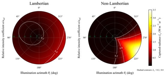
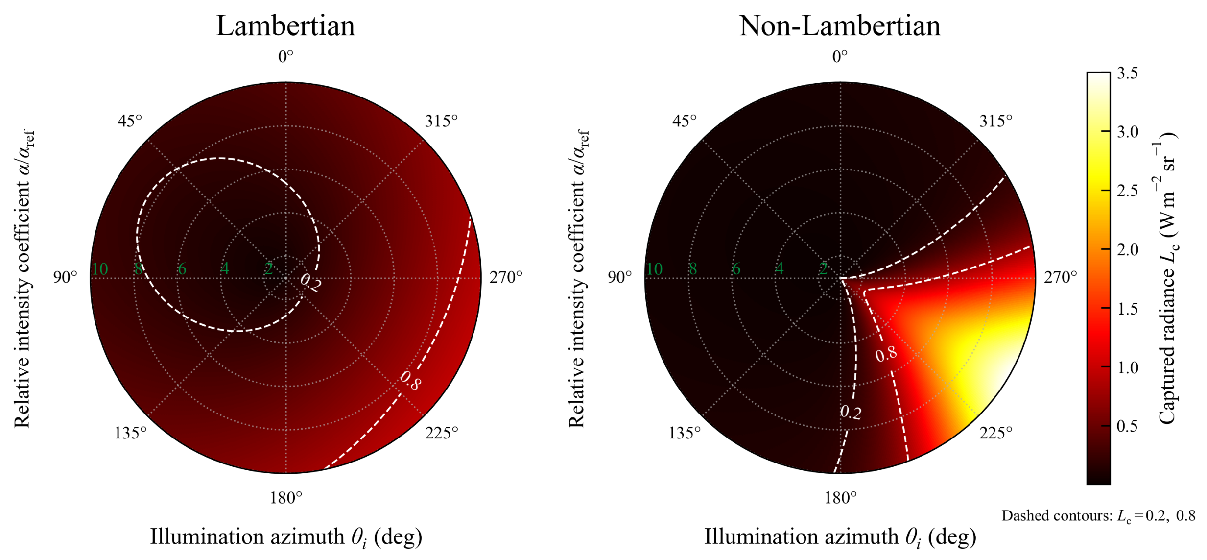
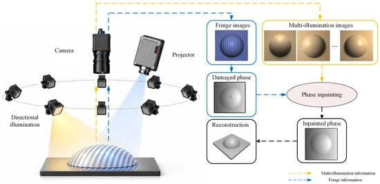
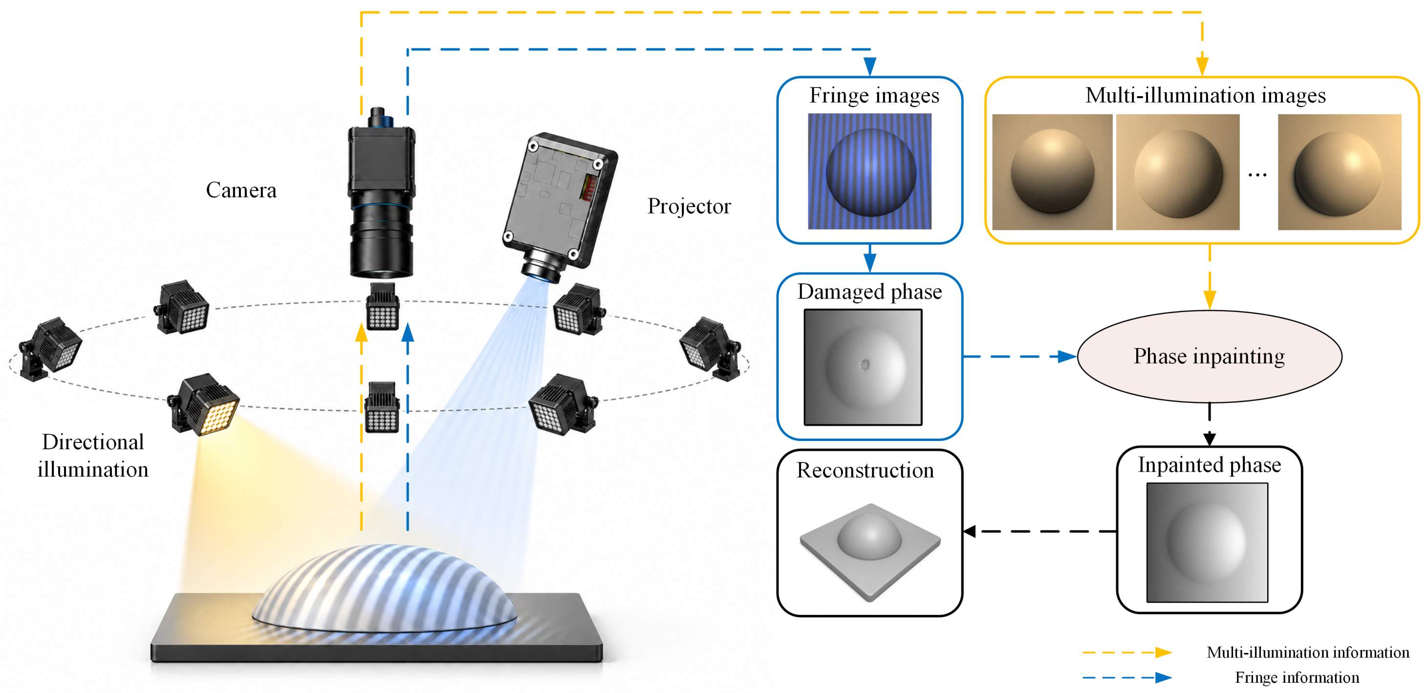
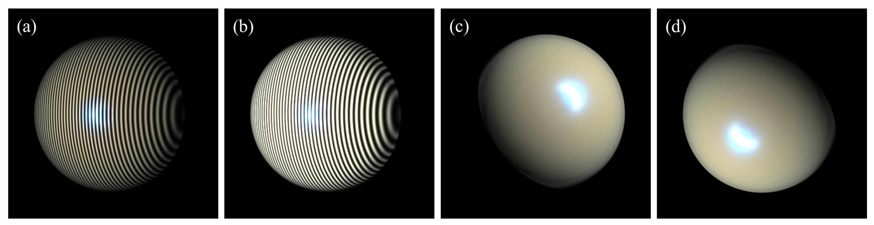
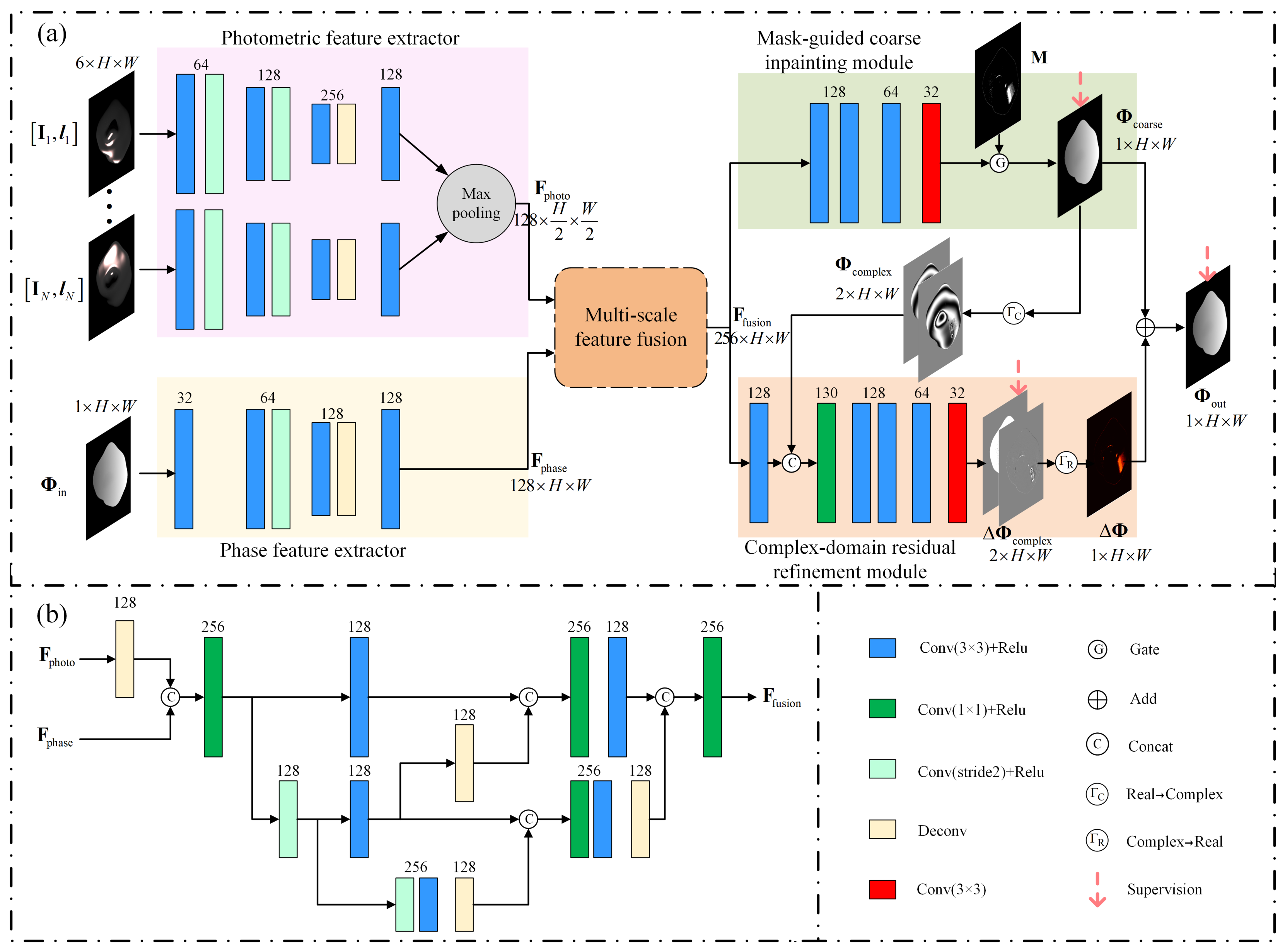
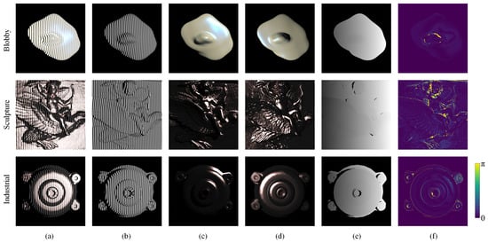
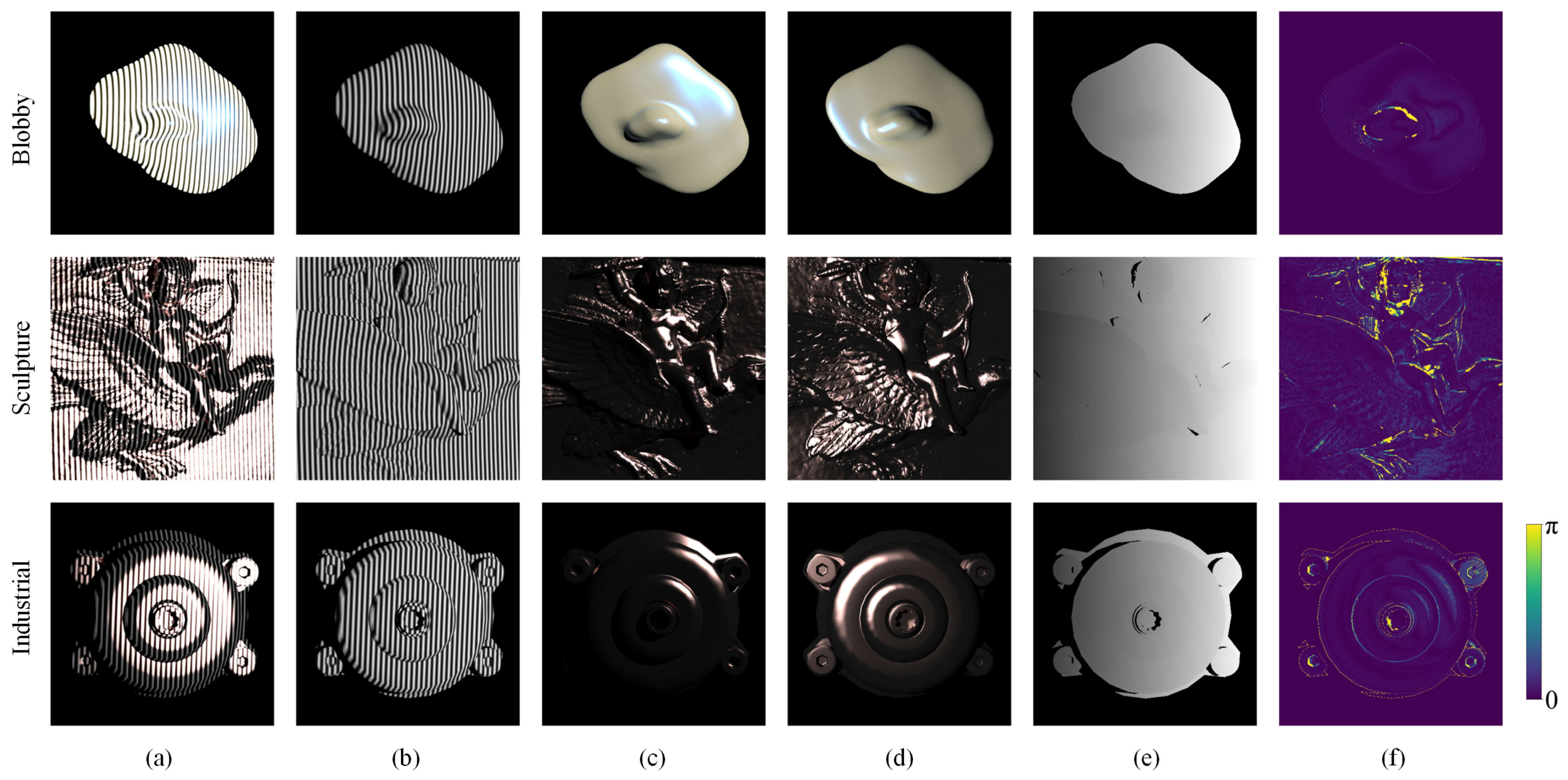
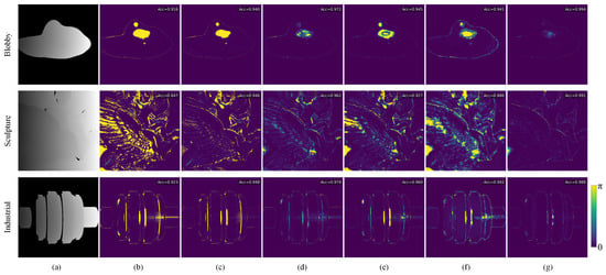
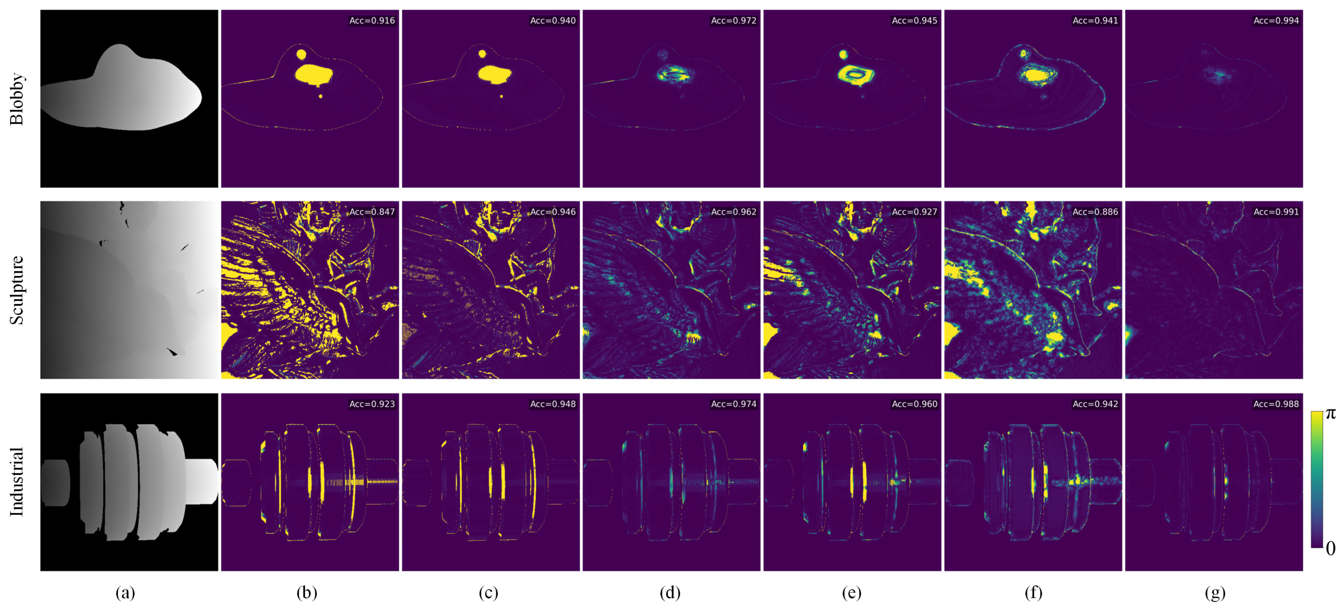
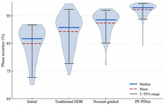
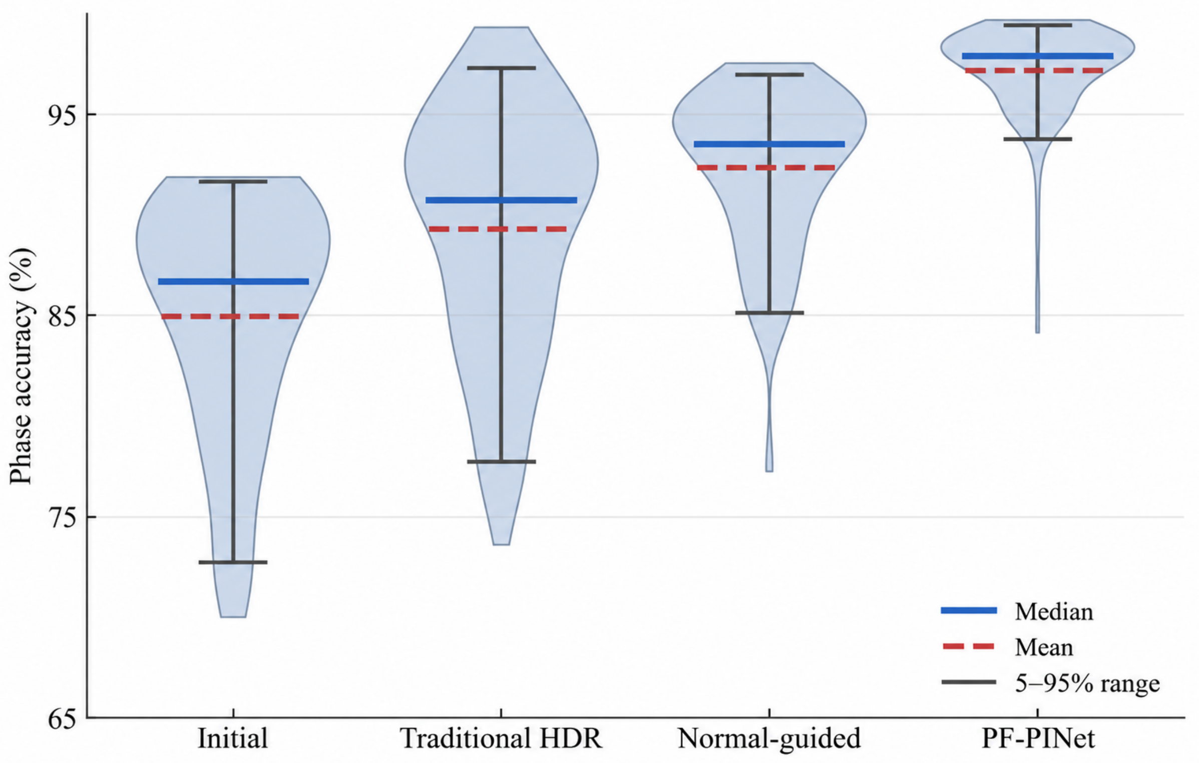


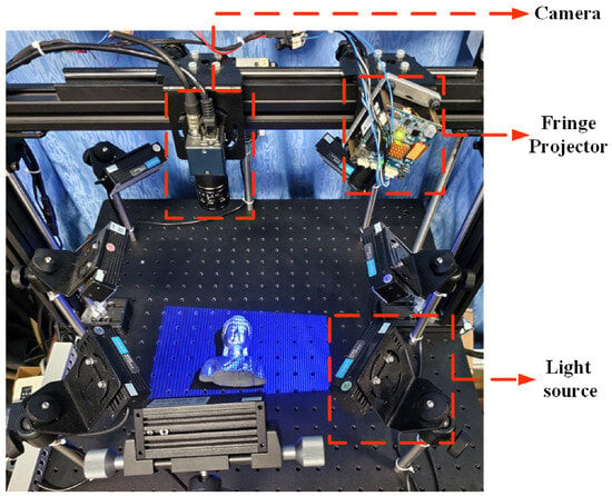
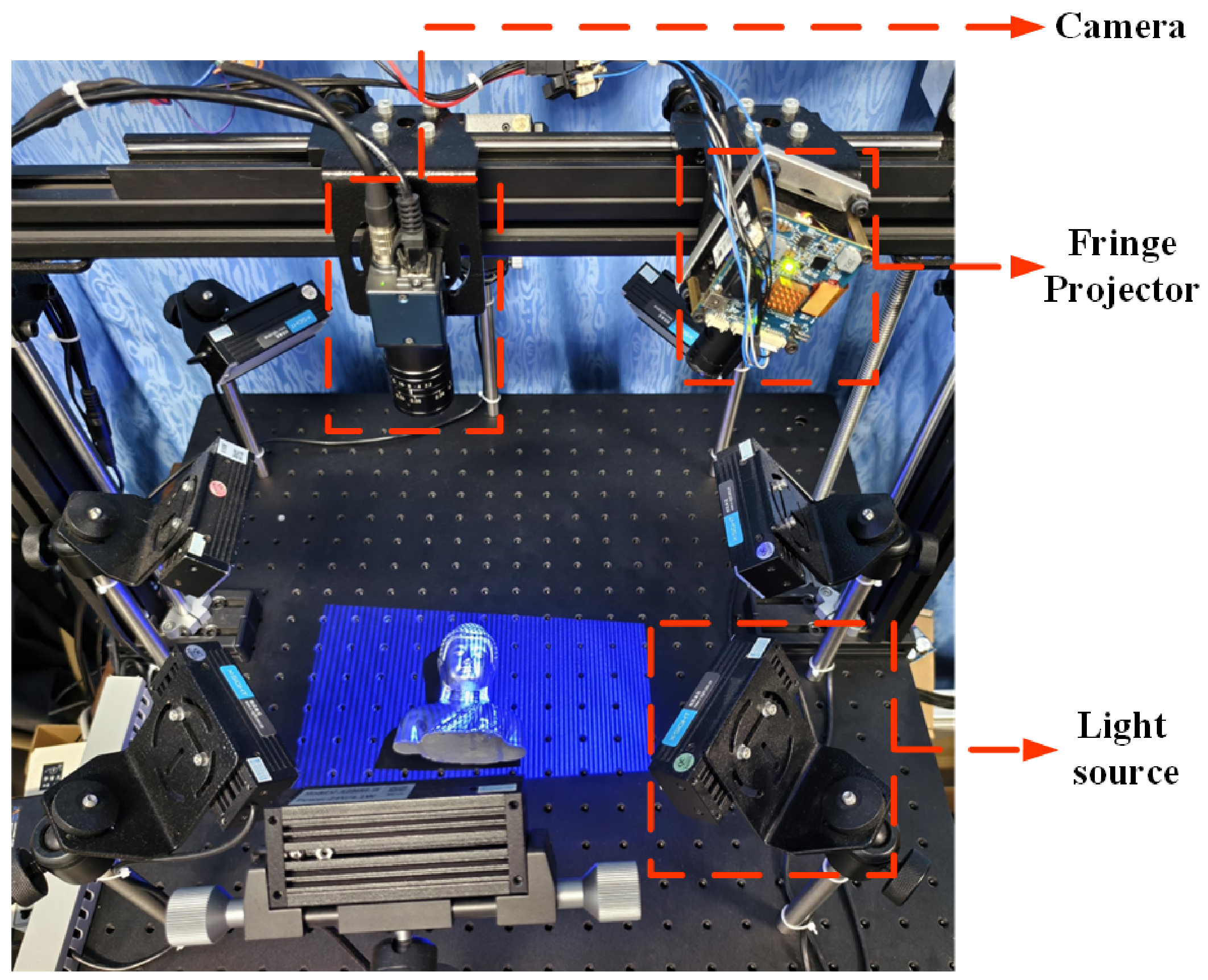
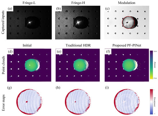
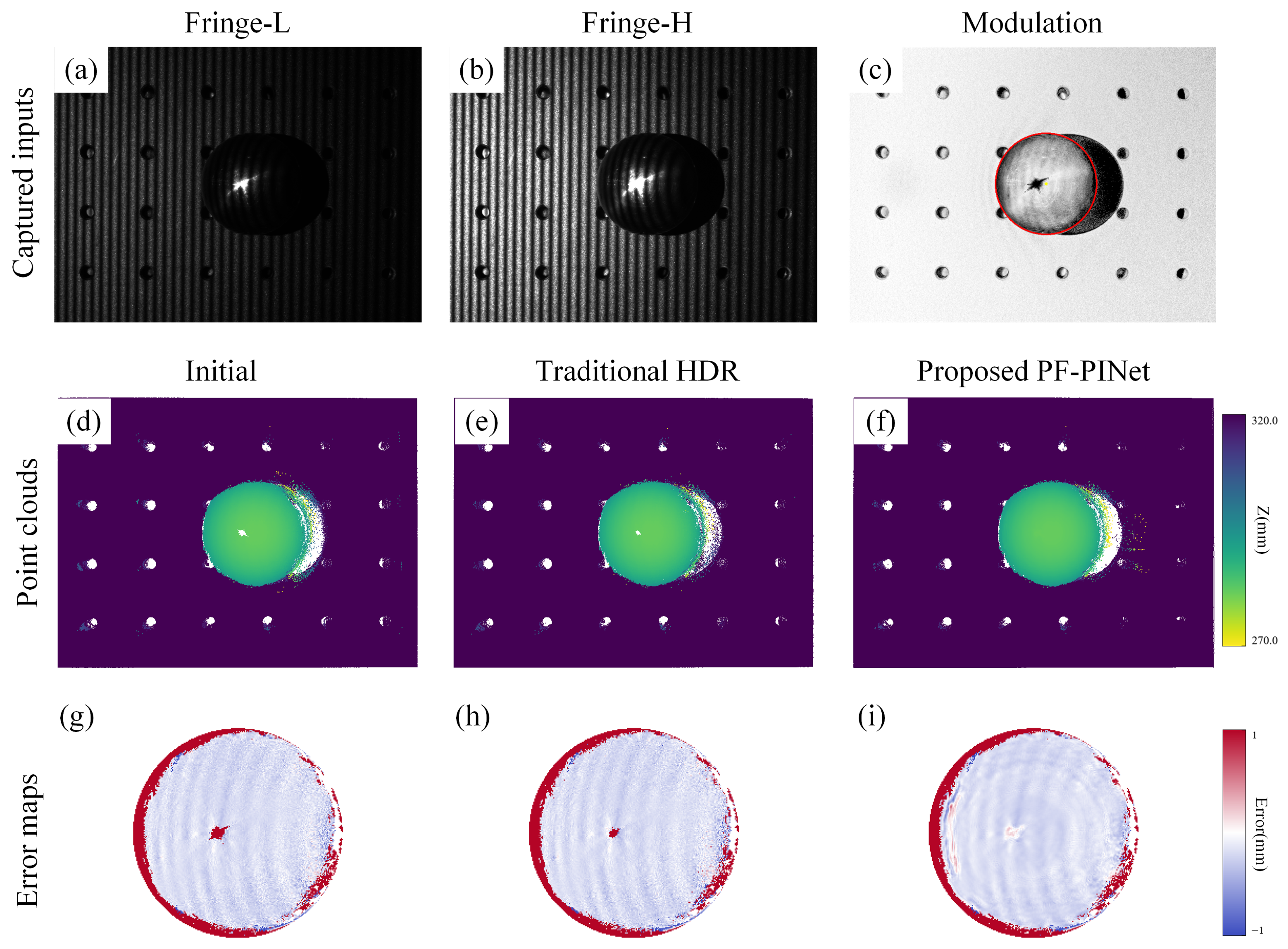
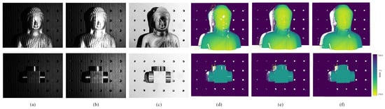
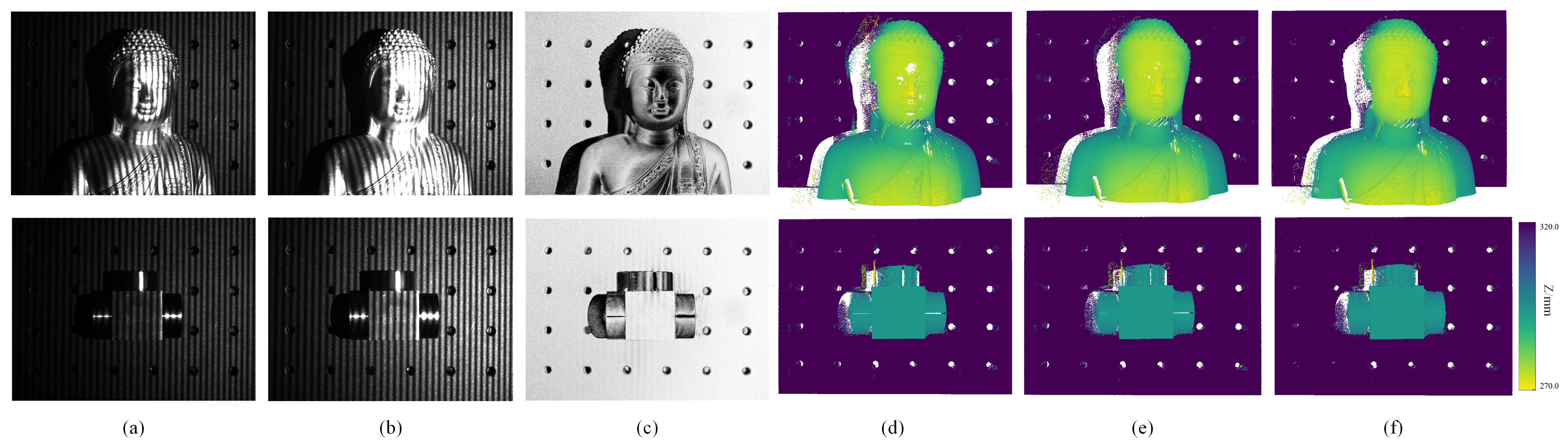

Disclaimer/Publisher’s Note: The statements, opinions and data contained in all publications are solely those of the individual author(s) and contributor(s) and not of MDPI and/or the editor(s). MDPI and/or the editor(s) disclaim responsibility for any injury to people or property resulting from any ideas, methods, instructions or products referred to in the content. |
© 2026 by the authors. Licensee MDPI, Basel, Switzerland. This article is an open access article distributed under the terms and conditions of the Creative Commons Attribution (CC BY) license.