Structural Consistency-Aware LiDAR Super-Resolution Method

Abstract

Existing LiDAR super-resolution methods primarily aim to increase point cloud density or improve coordinate reconstruction accuracy. However, they tend to introduce blurred edges and distorted planar surfaces during reconstruction, making it difficult to preserve the consistency of local scene geometry. To address this issue, this paper proposes a structural consistency-aware LiDAR super-resolution method that aims to preserve the local geometric relationships of the reconstructed point cloud with respect to the ground-truth point cloud in edge and planar regions. Specifically, complementary observations from adjacent frames are first fused using multi-scale dilated convolutions. An anisotropic Swin Transformer and a Coordinate-Aware Structure Enhancement (CASE) module are then employed to accommodate the horizontally dense and vertically sparse sampling pattern of LiDAR, strengthen long-range geometric modeling, and reduce the loss of critical structural information. During training, a local curvature-based structural consistency loss is designed to separately constrain edge sharpness and planar smoothness. During inference, prediction uncertainty and point cloud height are combined to adaptively remove low-confidence points, further improving the geometric reliability of the reconstructed point cloud. Experiments on the KITTI dataset show that the proposed method achieves an MAE of 0.4916 and an IoU of 0.4633, outperforming the representative comparison methods on both metrics. When the reconstructed point clouds are applied to A-LOAM, the average RTE and RRE values are reduced by 34.6% and 31.2%, respectively. In addition, experiments on the self-collected CSU-SLAM dataset provide preliminary evidence of the applicability of the proposed method to indoor and outdoor scenes under a different LiDAR configuration.

1. Introduction

LiDAR serves as a core sensor for environment perception in mobile robotics and autonomous driving systems, with its output 3D point clouds providing an essential foundation for high-precision scene understanding and downstream tasks [1]. High-resolution point clouds can finely represent the geometric structure of the environment and provide dense and stable spatial topological information, playing a critical role in tasks such as 3D reconstruction and object detection [2]. However, the physical resolution of LiDAR, especially the number of vertical scanning lines, which is strongly correlated with cost, is limited by sensor hardware architecture and manufacturing expenses. High-resolution devices therefore remain expensive and difficult to deploy on a large scale [3]. Consequently, utilizing algorithmic means to improve point cloud resolution on low-cost sensor platforms has become an important approach to balancing system cost and perception performance, driving the development of LiDAR super-resolution technology [4,5].

Given the rotational scanning mechanism of LiDAR, existing methods typically project 3D point clouds into 2D range images [6], thereby transforming the problem into a more mature 2D image super-resolution task. Based on the modeling approach, related methods are primarily categorized into implicit and explicit types. Implicit methods achieve high-resolution reconstruction by learning local interpolation functions of low-resolution images. While they offer flexibility for arbitrary scale factors, they tend to introduce blurring and structural distortion at complex geometric boundaries [7]. Explicit methods, which learn the end-to-end mapping relationship between low-resolution and high-resolution representations, offer higher reconstruction fidelity at fixed scales and have thus become the current mainstream technical route [8]. Nevertheless, most existing methods focus on increasing spatial density as the primary optimization objective. In SLAM applications, an increase in spatial density does not necessarily lead to improved localization performance. Particularly in feature-based SLAM frameworks, system performance highly depends on the clarity and stability of structural features, and existing methods struggle to effectively translate the reconstruction gains of super-resolution into enhanced localization accuracy [9].

However, simply increasing point cloud density does not necessarily lead to accurate recovery of scene geometry. In critical regions such as edges and planar surfaces, super-resolution reconstruction may introduce blurred boundaries, surface fluctuations, or outliers. Even when the global range error is low, these artifacts can disrupt local spatial relationships and cause geometric distortion. In this paper, structural consistency refers to the degree to which a reconstructed point cloud agrees with the ground-truth point cloud in terms of edge continuity, planar smoothness, and local structural stability within these critical regions. For downstream tasks such as LiDAR SLAM, reliable geometric features are essential for pose estimation. If super-resolution focuses only on increasing point density while neglecting structural consistency, improvements in reconstruction accuracy may not translate into better localization performance. Therefore, effectively preserving structural consistency during super-resolution reconstruction remains an important problem in LiDAR super-resolution [10].

To address these challenges, this paper proposes a structural consistency-aware LiDAR super-resolution method. The proposed method consists of four modules: Multi-scale Dilated Convolution Fusion (MDCF), anisotropic Swin Transformer encoding, Coordinate-Aware Structure Enhancement (CASE), and uncertainty-guided adaptive filtering. Furthermore, a structural consistency loss function is introduced, enabling the super-resolution reconstruction process to explicitly focus on preserving the integrity of critical geometric structures. The specific contributions are as follows:

(1)

A structural consistency-aware LiDAR point cloud super-resolution framework is proposed. By incorporating local geometric structure preservation into the super-resolution objective, the framework jointly optimizes range prediction accuracy and geometric integrity.

(2)

A feature extraction network is developed by integrating multi-frame temporal information, anisotropic global encoding, and coordinate-aware structure enhancement. By accounting for the scanning characteristics of LiDAR range images, the network strengthens long-range geometric dependency modeling and improves the recovery of critical structural information.

(3)

A structural consistency loss and an uncertainty-guided height-adaptive filtering module are designed to improve the recovery of critical geometric structures during training and output refinement, respectively.

2. Related Work

2.1. Implicit Methods

Implicit methods formulate LiDAR point cloud super-resolution as a continuous function-learning problem and reconstruct data at arbitrary scales by predicting the range value at any queried coordinate. This formulation provides a continuous representation and flexible upsampling ratios. LIIF [11] first introduced a local implicit image function that learns the mapping between local features and continuous coordinates, enabling high-accuracy prediction in continuous space. ILN [7] subsequently extended implicit representation to LiDAR super-resolution and improved reconstruction accuracy by modeling local interpolation relationships in the laser scanning process. IPN [12] further incorporated ray-position encoding to integrate LiDAR scanning directions and spatial positions into the implicit representation, thereby enhancing geometric modeling. Zhao et al. [13] proposed a self-supervised upsampling method based on implicit neural representations, enabling multi-scale point cloud reconstruction without high-resolution annotations and improving model generalization. WIN [4] constructed orthogonal virtual views in the horizontal and vertical directions and used complementary multi-view information to improve geometric recovery in complex regions. Overall, implicit methods mainly improve reconstruction accuracy through continuous representation learning. However, their objectives still focus on local interpolation or range prediction errors and lack explicit constraints on local geometric relationships such as edge continuity and planar smoothness. Consequently, over-smoothed regions and structural distortion may still occur in areas with abrupt geometric changes, making it difficult to preserve structural consistency between the reconstructed and ground-truth point clouds [14].

2.2. Explicit Methods

Explicit methods learn an end-to-end mapping from low-resolution to high-resolution range images. They generally provide higher reconstruction accuracy at fixed upsampling ratios and have therefore become a mainstream direction in LiDAR super-resolution. Triess et al. [15] first applied convolutional neural networks to scene-level LiDAR super-resolution and generated high-resolution point clouds by learning range-image mappings. LiDAR-SR [16] employed a U-Net architecture for range-image reconstruction and combined Monte Carlo Dropout with an outlier rejection strategy to suppress prediction noise and artifacts, improving output reliability. Chen et al. [17] introduced a channel-attention mechanism into a CNN to adaptively enhance the representation of critical features. TULIP [8] further applied the Swin Transformer to LiDAR super-resolution and used self-attention to strengthen long-range dependency modeling, thereby improving reconstruction in complex geometric regions. In addition, Tian et al. [18] combined semantic segmentation with geometric analysis and designed category-specific reconstruction strategies, whereas Jung et al. [19] jointly considered real-time inference and prediction uncertainty to achieve efficient and reliable LiDAR super-resolution.

Compared with implicit methods, explicit methods have stronger global feature modeling capabilities and generally perform better in range prediction accuracy. Nevertheless, most existing methods focus on network architecture and feature representation, while their training objectives still rely primarily on pixel-wise L1, L2, or similar range losses and thus lack direct constraints on local geometric relationships. Although attention mechanisms, Transformer architectures, and semantic information can improve feature representation, they do not explicitly guarantee the consistency of critical geometric structures. As a result, problems such as blurred edges and distorted planar surfaces remain [20].

3. Methodology

3.1. System Overview

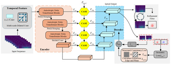
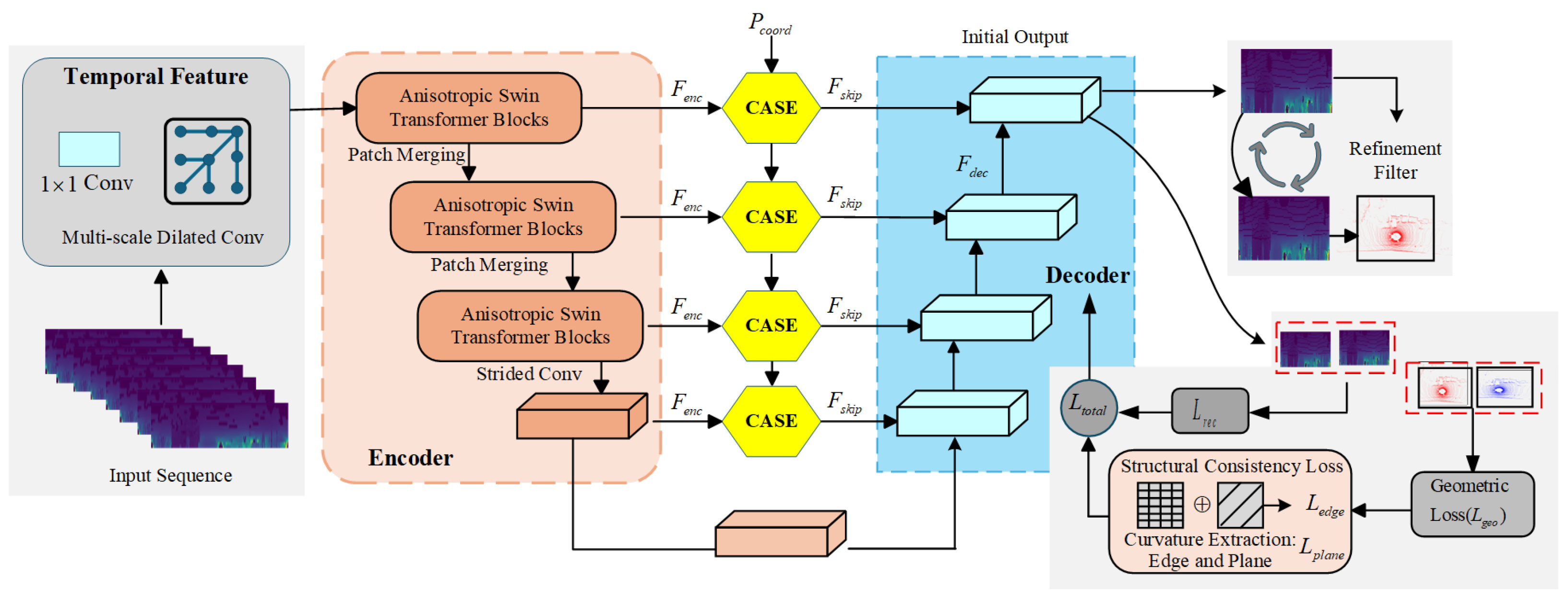
This paper proposes a structural consistency-aware LiDAR point cloud super-resolution method, whose overall architecture is illustrated in Figure 1. The system takes consecutive multi-frame range images as input. The MDCF module first uses temporal redundancy to compensate for spatial sampling sparsity and obtain a more complete temporal feature representation. The fused features are then fed into an anisotropic Swin Transformer encoder to model long-range geometric dependencies and structural topology in the point cloud. In the skip connections between the encoder and decoder, a CASE module embeds physical-coordinate priors into feature propagation, enhancing local structural information and improving the preservation of critical geometric structures. The decoder reconstructs the high-resolution range image. During training, a local curvature-based structural consistency loss explicitly constrains critical edge and planar features to jointly optimize reconstruction accuracy and geometric consistency. During inference, an uncertainty-guided height-adaptive filtering module suppresses and removes high-uncertainty regions, thereby reducing artifacts and producing super-resolved point clouds with higher geometric consistency.

Figure 1. System overview.

3.2. Multi-Frame Temporal Feature Extraction

In a single LiDAR scan frame, the point clouds often suffer from insufficient geometric information and physical occlusions due to the inherent spatial sparsity of scanning lines, especially in long-range regions. To address this, we introduce continuous multi-frame temporal data as input, leveraging redundant observations in the temporal dimension to compensate for sparsity in the spatial dimension, thereby enhancing the completeness and robustness of scene representation.

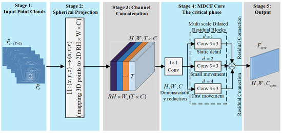
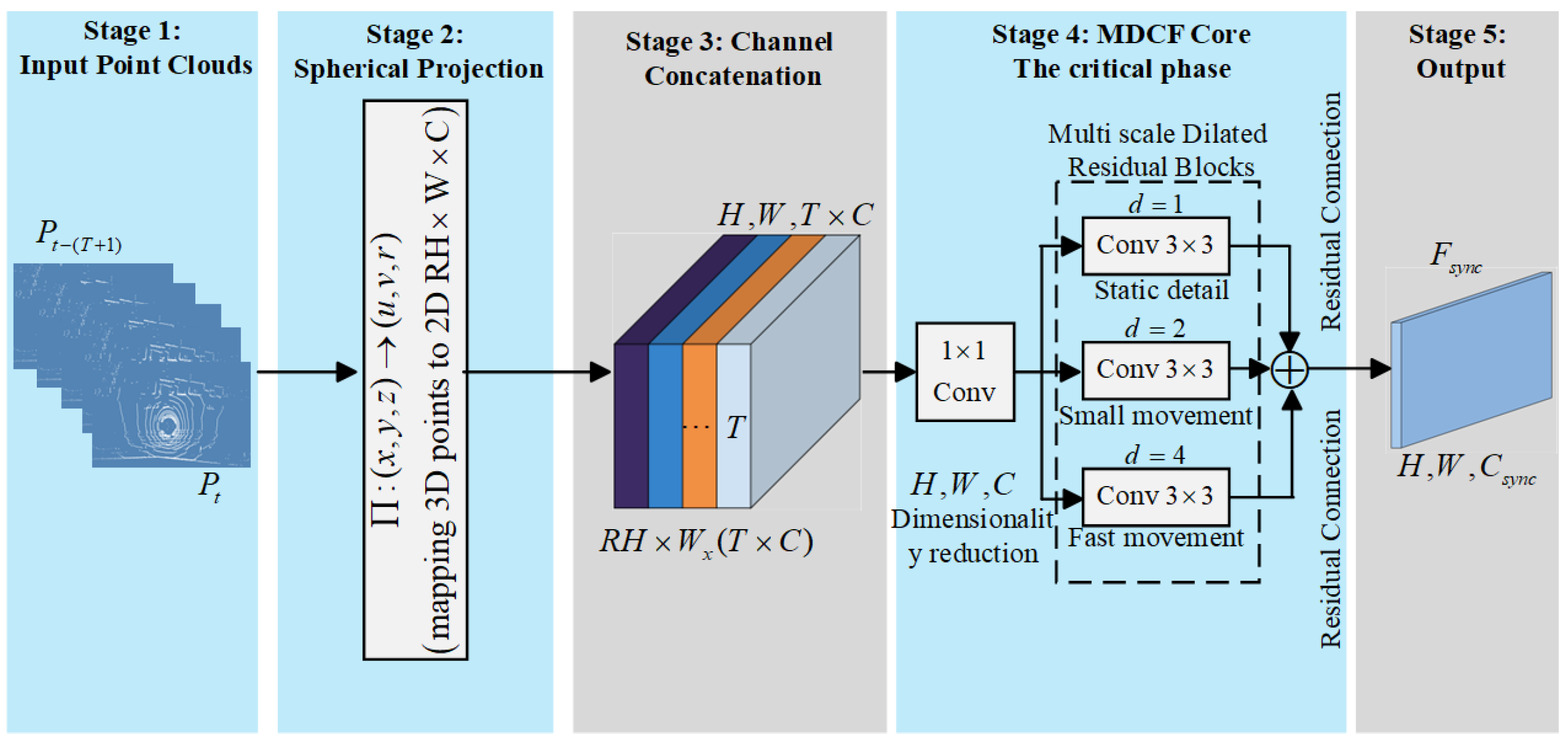
As illustrated in Figure 2, unordered 3D point clouds are first mapped into a 2D image space via spherical projection. For any point $p_i\left(x,y,z\right)$, it is converted into pixel coordinates $\left(u,v\right)$ on the range image [7]:

$$\left\{\begin{array}{c}u={\displaystyle \frac{1}{2}}\left[1-\arctan \left(y,x\right)/\pi \right]\cdot W\\ v=\left[1-\left(\arcsin \left(z/r\right)+f_{up}\right)/f\right]\cdot H\end{array}\right.$$

(1)

where $r=\sqrt{x^2+y^2+z^2}$ represents the range from the point to the sensor, $H$ and $W$ are the height and width of the projected image, and $f$ denotes the total vertical Field of View (FoV) of the sensor. $f_{up}$ represents the upper boundary bias of the FoV, used for vertical coordinate system calibration.

Figure 2. Schematic Diagram of Multi-Frame Temporal Feature Extraction.

Before multi-frame temporal fusion, ego-motion compensation is performed. Taking frame $t$ as the reference frame, other point cloud frames are transformed into the reference frame according to their relative poses and then re-projected onto the spherical range-image grid using Equation (1), thereby unifying the geometric reference frame across different timestamps before feature fusion.

For a sequence of $T$ consecutive range image frames $\left\{I_1,I_2,\dots ,I_T\right\}$, after ego-motion compensation and re-projection, the resulting range images are concatenated along the channel dimension to form the initial input tensor $X=Comcat\left(I_1,I_2,\dots ,I_T\right)$.

Subsequently, a $1\times 1$ convolutional layer is employed for feature embedding, mapping raw physical observations into a high-dimensional feature space to achieve preliminary cross-channel information fusion while compressing temporal redundancy. Although ego-motion compensation substantially reduces the geometric displacement caused by platform motion, residual inter-frame inconsistencies may still remain due to pose errors, viewpoint changes, occlusions, and dynamic objects. Standard convolutions, limited by their local receptive fields, have limited capability to model such residual spatial variations and complementary observations across frames. To address this issue, an MDCF module is designed in this work. Based on the embedded features, this module processes data through parallel multi-branch $3\times 3$ convolutions with different dilation rates $d\in \left\{1,2,4\right\}$. Specifically, branches with smaller dilation rates are used to preserve local details, while branches with larger dilation rates capture residual spatial variations and complementary structural information across temporally aligned frames. Finally, features from each branch are weighted and fused via residual connections to generate a spatial-consistency-enhanced feature map $F_{md}$, which serves as the input for subsequent modules.

3.3. Global Feature Encoding Based on Anisotropic Swin Transformer

Global feature encoding aims to fully model the geometric distribution characteristics and long-range topological dependencies of point clouds, providing stable and highly discriminative feature support for subsequent reconstruction. Influenced by the rotational scanning mechanism of LiDAR, point clouds exhibit continuous and dense sampling in the horizontal direction, while displaying significant discrete sparsity in the vertical direction due to the fixed number of scanning lines. Traditional Swin Transformers employ square attention windows and uniform token partitioning, which tend to introduce cross-vertical information mixing during the early stages of feature extraction, thereby weakening the representation of critical structures [9]. To address this, this paper designs an anisotropic Swin Transformer encoder, specifically optimized in terms of token partitioning, attention windows, and shifting strategies:

Firstly, the input feature map $F_{md}$ is partitioned into elongated tokens of size $1\times P_w$, where $P_w$ denotes the horizontal partitioning stride. This partitioning method ensures that each processing unit contains only consecutive observations within the same scan line, effectively avoiding premature fusion of vertical features.

Subsequently, in the self-attention calculation, the conventional square window is adjusted to an elongated window of size $M_h\times M_w$, which is set to 1 × 16 in our implementation, with the constraint $M_h\ll M_w$ strictly enforced. This design significantly expands the receptive field of the attention mechanism in the horizontal direction, enabling the model to capture long-distance geometric correlations and more accurately perceive horizontally extended structural information.

Finally, to break the isolation between local windows, a purely horizontal window shifting mechanism is proposed. Elongated windows and horizontally shifted windows are used alternately in consecutive encoding blocks. Specifically, the standard window is used for local feature modeling, while the shifted window cyclically shifts to the right by $M_w/2$ only in the horizontal direction, without any vertical offset. This strategy enables cross-window information transfer within the same scan line, thereby enhancing global modeling capabilities while maintaining vertical structural consistency.

3.4. Coordinate-Aware Structure Enhancement Module

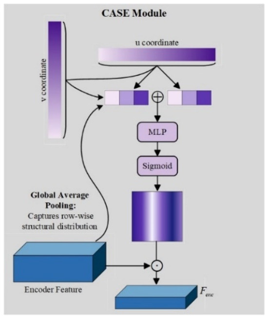
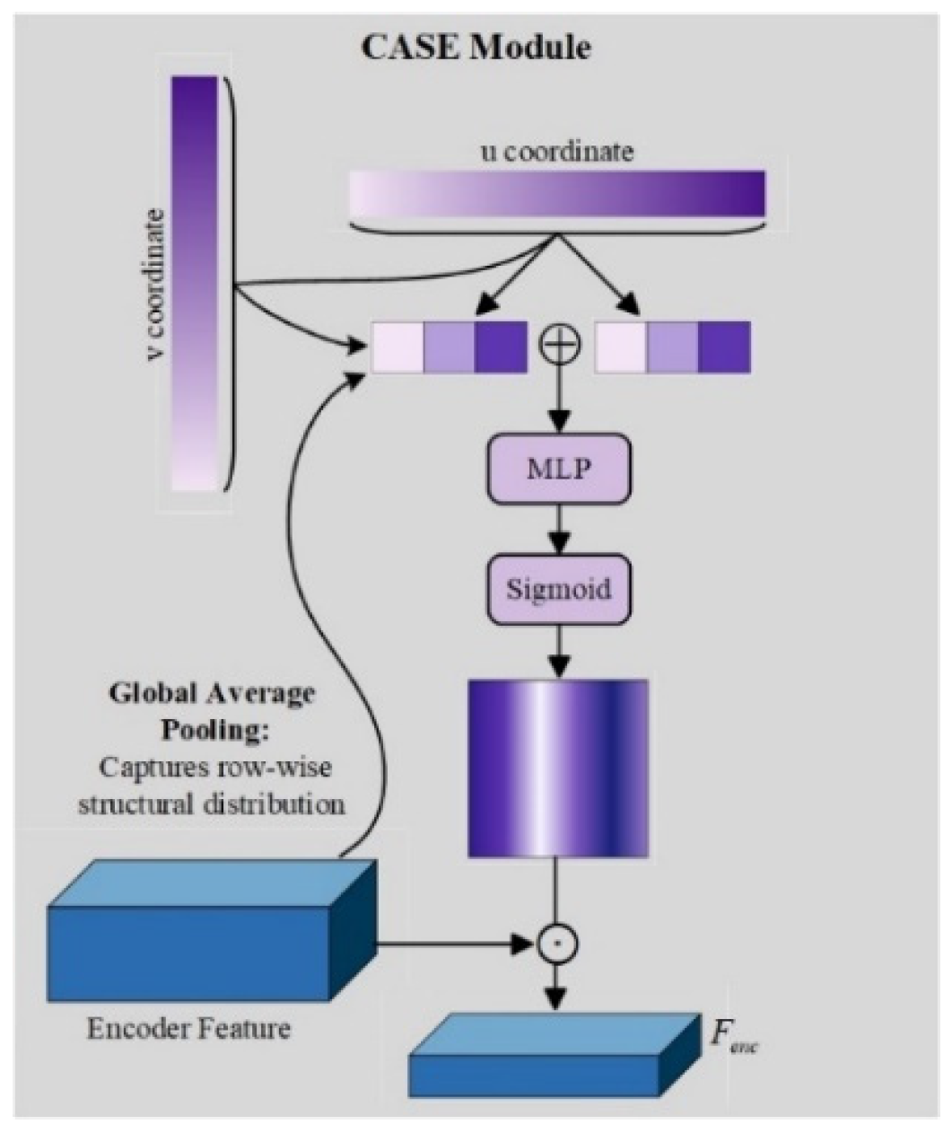
Although the anisotropic Swin Transformer can efficiently model horizontal geometric features, the overlapping receptive fields and feature fusion during the continuous downsampling process of the U-Net encoding stage lead to aliasing and resolution loss of fine vertical geometric features. Furthermore, standard skip connections only perform channel concatenation between encoder and decoder features, lacking explicit guidance and calibration for geometric structures. To address this, this paper designs a CASE module within the skip connection path, which guides the decoder to prioritize the reconstruction of key regions with geometric consistency by transforming physical coordinate priors of point clouds into spatial attention weights. As illustrated in Figure 3, the specific workflow is as follows:

Figure 3. Schematic diagram of CASE module.

Firstly, the vertical structure vector is extracted. For the feature map $F_{enc}\in R^{B\times C_l\times H_l\times W_l}$ of the $l$-th layer in the encoder, global average pooling is performed along the horizontal direction to obtain a vector $V_{vert}$ that reflects the overall structural distribution in the vertical direction, where $B$, $C_l$, $H_l$, and $W_l$ denote the batch size, number of channels, feature-map height, and feature-map width, respectively. This vector encodes the average response intensity of each scan line, roughly capturing the geometric information density at different height levels.

Subsequently, the absolute coordinate prior is injected. To provide an accurate spatial position reference, a standardized coordinate tensor $P_{coord}$ is constructed, with its two channels storing the normalized horizontal and vertical coordinates of each pixel, respectively. This coordinate tensor provides the network with absolute positional information for feature points within the original projected image.

Then, the spatial attention map is generated. The spatial dimensions of the vertical structure vector $V_{vert}$ are expanded to match the original feature map, resulting in $V_{vert}^{\prime }$. $V_{vert}^{\prime }$ and the coordinate tensor $P_{coord}$ are concatenated along the channel dimension to form a tensor that fuses semantic features and spatial positions. This fused tensor is processed by a lightweight Multi-Layer Perceptron (MLP) to learn and generate a spatial attention weight map $M_{case}$:

$$M_{case}=\sigma \left(MLP\left(\left[V_{vert}^{\prime };P_{coord}\right]\right)\right)$$

(2)

where $\sigma$ denotes the sigmoid activation function. The MLP maps the channel dimension of the input tensor from $C_l+2$ to 1 in a pixel-wise manner.

Finally, feature calibration and transmission are performed. The generated spatial attention map is used for pixel-level weighting of the original encoder features to obtain the calibrated skip connection features:

$$F_{skip}^l=F_{enc}^l\odot M_{case}$$

(3)

where $\odot$ represents element-wise multiplication. The calibrated features $F_{skip}^l$ are then transmitted to the corresponding layer of the decoder for upsampling and feature fusion.

By guiding the decoder with geometrically enhanced features, this module prioritizes the preservation of key vertical edges and structures with physical consistency during the reconstruction process, thereby improving geometric reconstruction accuracy in complex scenarios.

3.5. Uncertainty-Guided Height-Adaptive Filtering

After processing by the aforementioned modules, the network generates a preliminary high-resolution image. However, due to factors such as sensor noise and motion ghosting from dynamic objects, geometric artifacts and regions of high uncertainty inevitably exist in the predicted results. If these unreliable regions are not effectively identified and removed, the geometric reliability of the reconstructed point clouds will be degraded, thereby affecting the accuracy of subsequent point cloud processing tasks. To address this, this paper proposes an uncertainty-guided height-adaptive filtering module that identifies and removes unreliable predicted points by quantifying the uncertainty of model predictions.

First, an MC Dropout method is employed, where the dropout layers remain active during the inference stage, and $N$ random forward passes are performed on the same input sequence to generate multiple sets of range image prediction samples [17].

Subsequently, the sample variance ${\sigma }^2\left(u,v\right)$ of the predicted values at each pixel location is calculated to describe the dispersion of the model’s prediction results. A larger variance indicates poorer stability in the model’s prediction for that specific point. After normalizing the variance, a normalized confidence map $M_{prob}$ representing the existence of a true and reliable point at each pixel location is obtained:

$$M_{prob}\left(u,v\right)=1-{\displaystyle \frac{{\sigma }^2\left(u,v\right)}{\max \left({\sigma }^2\right)}}$$

(4)

This normalization does not require a predefined variance scale, can adapt to each input sample, and preserves the monotonic relationship that a larger variance corresponds to a lower confidence score. In addition, normalization is performed only at locations with valid range predictions, thereby avoiding interference from invalid pixels.

The reliability of point cloud prediction is jointly affected by several factors, such as measurement noise and the laser incidence angle. These factors have complex distributions in the range-image domain, making it difficult to establish a unified explicit mapping. In contrast, point height has a clear physical and topological relationship with the ground: near-ground regions usually correspond to stable static structures, whereas elevated regions are more susceptible to sparse noise caused by atmospheric scattering, multipath effects, and limited angular resolution [14]. Therefore, height is used as the control variable of the adaptive threshold to model differences in artifact distributions across elevation ranges more directly. Specifically, the filtering threshold $\tau$ is defined as a nonlinear function of the height $z$:

$$\tau \left(z\right)={\tau }_{\min }+\left({\tau }_{\max }-{\tau }_{\min }\right)\cdot \sigma \left(\gamma \cdot \left(z-z_{ref}\right)\right)$$

(5)

where $z_{ref}$ represents the ground reference height, ${\tau }_{\max }$ and ${\tau }_{\min }$ set the upper and lower bounds for confidence filtering, respectively, and $\gamma$ is a scale factor controlling the steepness of the function. Compared with an unbounded linear or exponential function, the sigmoid function has explicit lower and upper asymptotes, ensuring that the filtering threshold always remains within the prescribed bounds and reducing abrupt changes in filtering strength between adjacent spatial regions.

Finally, the system combines the confidence map with the height-adaptive threshold to perform pixel-wise determination. A reconstructed 3D point is retained only when its confidence score satisfies $M_{prob}>\tau \left(z\right)$; all remaining low-confidence predictions are regarded as artifacts and removed.

3.6. Geometric Structural Consistency Loss Function Design

LiDAR super-resolution networks typically prioritize coordinate reconstruction accuracy as the core optimization objective, utilizing loss functions such as $L1$ or $L2$ to minimize the Euclidean distance deviation between predicted and ground-truth points. However, simply improving pixel-level range accuracy is insufficient to guarantee the geometric quality of the reconstructed point clouds. Even minor distortions in local geometry may lead to blurred edges, inflated planes, or generated artifacts, significantly degrading the structural consistency of the point clouds. Accordingly, a local curvature-based structural consistency loss is introduced to further constrain the geometric agreement between the reconstructed and ground-truth point clouds while optimizing coordinate accuracy.

Local curvature effectively describes the degree of geometric variation on a point cloud surface. High-curvature regions generally correspond to geometric discontinuities such as edges and corners, whereas low-curvature regions generally correspond to planar or ground surfaces. Therefore, the curvature distribution provides a concise representation of local point cloud geometry. When a super-resolved point cloud maintains a curvature distribution consistent with that of the ground-truth point cloud, critical structures such as edges and planar surfaces can be preserved more effectively. This idea is also consistent with curvature-based feature extraction in SLAM methods such as LOAM [21]. To calculate structural consistency, the predicted and ground-truth range images are first back-projected into their corresponding 3D point clouds. Following the feature extraction strategy of LOAM, the local curvature of each valid 3D point is calculated using neighboring points on the same LiDAR scan line:

$$c={\displaystyle \frac{1}{\left|S\right|\cdot ‖x_i‖}}‖{\displaystyle \sum _{j\in S,j\ne i}\left(x_j-x_i\right)}‖$$

(6)

where $S$ denotes the local neighborhood of point $p_i$ on the same LiDAR scan line, consisting of the five preceding and five succeeding valid points, and $x$ denotes the 3D coordinate vector. Only points with a complete valid neighborhood are considered; invalid points and points located within the first or last five positions of each scan line are excluded from the curvature calculation.

According to the LOAM feature extraction criterion, points with curvature values greater than 0.1 are classified as edge candidates, whereas those with curvature values less than 0.1 are classified as planar candidates. The edge point set $\epsilon$ and planar point set $H$ used for structural supervision are both extracted from the ground-truth point cloud, and the predicted and ground-truth curvature responses are compared at the corresponding locations. For these two types of features, an edge sharpness loss $L_{edge}$ and a planar smoothness loss $L_{plane}$ are designed. $L_{edge}$ constrains the curvature distribution of the predicted results in edge regions, forcing the network to maintain or enhance edge sharpness and preventing edge blurring or dilation caused by super-resolution:

$$L_{edge}={{\displaystyle \sum _{i\in \epsilon }‖c_i^{sr}-c_i^{gt}‖}}^2$$

(7)

where $c_i^{sr}$ and $c_i^{gt}$ denote the curvature values of the predicted and ground-truth point clouds at location i, respectively. This term is computed only over the edge-point set and encourages the prediction to preserve a relatively large local curvature response consistent with the target point cloud at ground-truth edge locations.

$L_{plane}$ constrains the local consistency of the predicted results in planar regions, encouraging the network to generate smooth and coherent planes while suppressing noise or outliers that might introduce pseudo-planar features:

$$L_{plane}={{\displaystyle \sum _{j\in H}‖c_j^{sr}-c_j^{gt}‖}}^2$$

(8)

This term is computed only over the planar-point set and encourages the prediction to maintain a small and stable local curvature response in ground-truth planar regions.

The structural consistency loss is defined as the weighted sum of the two:

$$L_{struct}=\alpha L_{edge}+\beta L_{plane}$$

(9)

where $\alpha$ and $\beta$ are weighting coefficients to balance the two loss terms.

Finally, by combining the traditional geometric coordinate reconstruction loss with the structural consistency loss, the overall training objective is obtained:

$$L_{total}={\lambda }_1{L}_{geo}+{\lambda }_2{L}_{struct}$$

(10)

where $L_{geo}$ is the $L1$ loss, and ${\lambda }_1$ and ${\lambda }_2$ are weighting coefficients used to balance the two loss terms.

4. Experiments

4.1. Experimental Setup

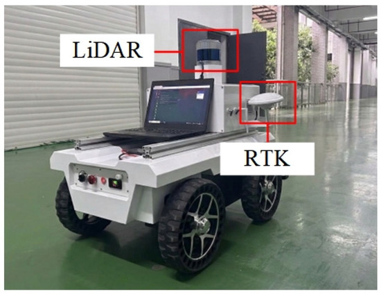
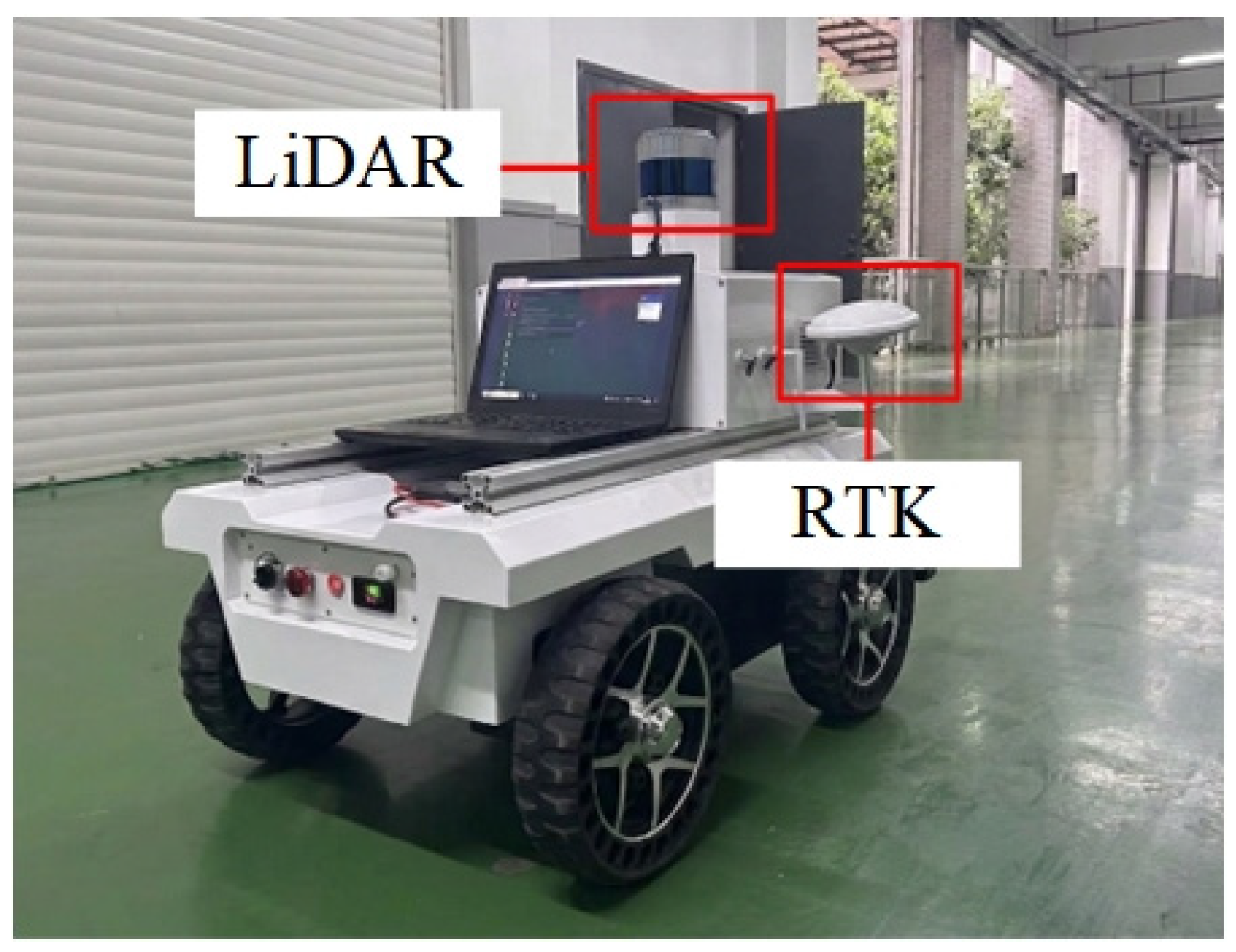
To comprehensively evaluate the performance of the proposed method, the KITTI dataset [22] is selected as the benchmark for training and testing. Additionally, a self-collected CSU-SLAM dataset is introduced to further evaluate the applicability of the proposed method under different sensor and scene conditions. The KITTI dataset is a classic open benchmark in the autonomous driving field, covering various urban road scenarios. Following common partitioning practices, sequences 00–08 are used as the training set, while sequences 09 and 10 serve as the test set. The CSU-SLAM dataset was collected on the campus of Central South University using the mobile robotic platform shown in Figure 4, which was equipped with a Leishen C16 LiDAR and a high-precision RTK system. Under normal conditions, the RTK system provides a positioning accuracy of approximately 1–5 cm. This dataset was used only for testing and was not involved in model training. The main specifications of the LiDAR are listed in Table 1.

Figure 4. Robot platform.

Table 1. Main specifications of the Leishen C16 LiDAR.

Specification	Value
Detection range	0.4–150 m
Ranging accuracy	±3 cm
Horizontal angular resolution	0.36°
Vertical angular resolution	2°
Scan rate	10 Hz

The input to the network consists of four consecutive low-resolution range images with a resolution of 16 × 1024, and the target high-resolution output has a resolution of 64 × 1024, corresponding to a 4× vertical upsampling ratio. Specifically, the original LiDAR point clouds are first projected into range images with a resolution of 64 × 1024. The low-resolution inputs are generated by uniformly downsampling one scan line out of every four in the vertical direction. The range values are normalized using a scale factor of 1/80, and missing or invalid measurements are filled with zero. During projection, measurements beyond 120 m are treated as invalid, while the effective prediction range is limited to 80 m during reconstruction and evaluation. In addition to the network architecture, the remaining key hyperparameters were selected by grid search on the validation set. The weights of the geometric reconstruction loss and structural consistency loss were set to ${\lambda }_1=0.87$ and ${\lambda }_2=0.51$, respectively. Within the structural consistency loss, the weights of the edge sharpness loss and planar smoothness loss were set to $\alpha =0.73$ and $\beta =0.34$, respectively. During inference, the dropout rate was set to 0.1, and 10 stochastic forward passes were performed to estimate prediction uncertainty. For the height-adaptive filtering module, the parameters were set to ${\tau }_{\min }=0.4$, ${\tau }_{\max }=0.75$, $z_{ref}=0.12$, and $\gamma =5$. The model was implemented in PyTorch (1.12.0) and trained on four NVIDIA GeForce RTX 3060 GPUs using the AdamW optimizer. The initial learning rate was 5 × 10⁻⁴, the model was trained for 200 epochs, and the batch size was 8. The main implementation parameters and training settings are summarized in Table 2.

Table 2. Detailed implementation parameters and training configurations of the model.

Parameters	Value	Parameters	Value
Input resolution	16 × 1024	Training epochs	200
Output resolution	64 × 1024	${\lambda }_1$$/{\lambda }_2$	0.87/0.51
Vertical upsampling ratio	4	$\alpha$ $\beta$	0.73/0.34
Number of input frames	4	Number of MC Dropout samples	10
$M_h\times M_w$	1 × 16	Dropout rate	0.1
$P_w$	16	${\tau }_{\min }$$/{\tau }_{\max }$	0.4/0.75
Optimizer	AdamW	$z_{ref}$	0.12
Initial learning rate	5 × 10−4	$\gamma$	5
Batch size	8	Parameter count	29.3 M

Representative methods in the current LiDAR super-resolution field, encompassing both implicit and explicit types, are selected as baselines for comparison. For explicit methods, the classic learning-based reconstruction method LiDAR-SR [16] and the Transformer-based method TULIP [8] are chosen; for implicit methods, the general approach LIIF [11], which supports arbitrary-scale upsampling, is selected. To ensure experimental fairness, all comparative methods utilize their official open-source implementations and are retrained on the same training set to unify the experimental baseline.

The evaluation metrics cover both super-resolution reconstruction and downstream-task performance. For super-resolution results, Mean Absolute Error (MAE) and Intersection over Union (IoU) are used as evaluation metrics. MAE is calculated as the mean absolute difference between the predicted and ground-truth range values over all pixels in the two-dimensional range image and measures the pixel-level reconstruction error. Since MAE is calculated directly from the normalized range values rather than from the range values restored to the metric scale, it is dimensionless. A smaller value indicates higher reconstruction accuracy. IoU quantifies the geometric consistency of the reconstructed point clouds by performing voxelization on both the predicted and ground-truth point clouds in 3D space and calculating the intersection over union of the occupied voxels; higher values signify better geometric fidelity. During evaluation, the predicted and ground-truth range images are first back-projected into 3D point clouds in the LiDAR coordinate frame, with a maximum range of 80 m. Both point clouds are then voxelized using a voxel size of 0.1 m. For each sample, the voxel-grid boundaries are jointly determined by the minimum and maximum coordinates of the predicted and ground-truth point clouds, and a voxel containing at least one point is considered occupied [4,8]. For downstream task performance, this paper selects A-LOAM, a classic LiDAR SLAM method in the field of robot navigation, for testing to verify the effectiveness of the super-resolved point clouds in practical applications. All SLAM experiments were conducted using the official A-LOAM implementation. The feature curvature threshold was set to 0.1, and each scan line was divided into six sectors for feature extraction. In each sector, at most 2 sharp-edge points, 20 less-sharp-edge points, and 4 planar points were selected. The maximum number of Ceres optimization iterations was set to 4. For the 64-line configuration, the voxel resolutions for mapping edge and planar features were set to 0.4 m and 0.8 m, respectively, and the mapping skip-frame parameter was set to 1. Under the same input configuration, all parameters were kept unchanged across different super-resolution methods. SLAM performance is assessed using Relative Pose Error (RPE) as the core metric, which includes two components: Relative Translation Error (RTE) and Relative Rotation Error (RRE). RPE measures the deviation between the estimated pose and the ground-truth pose within a fixed time interval, effectively reflecting the local cumulative drift characteristics of the SLAM system.

4.2. Validation on the KITTI Dataset

In this section, a quantitative validation of the super-resolution performance of the proposed method and the baseline models is conducted on the KITTI test set, with the results summarized in Table 3. The results show that the proposed method achieves the best performance in both MAE and IoU, improving upon the second-best method, TULIP, by approximately 7.6% and 12.7%, respectively. Specifically, the proposed method obtains an MAE of 0.4916, corresponding to a lower range prediction error and indicating higher range reconstruction accuracy. It also achieves an IoU of 0.4633, indicating greater structural agreement between the reconstructed and ground-truth point clouds and better preservation of critical scene geometry.

Table 3. Super-resolution performance results on the KITTI test set.

Methods	MAE	IoU
LIIF	0.6945	0.1397
LiDAR-SR	0.5720	0.4101
TULIP	0.5321	0.4112
Ours	0.4916	0.4633

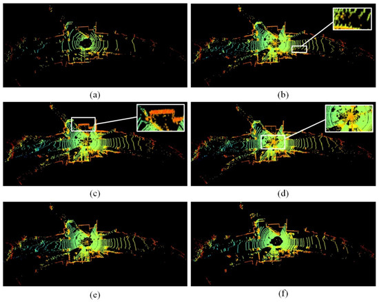
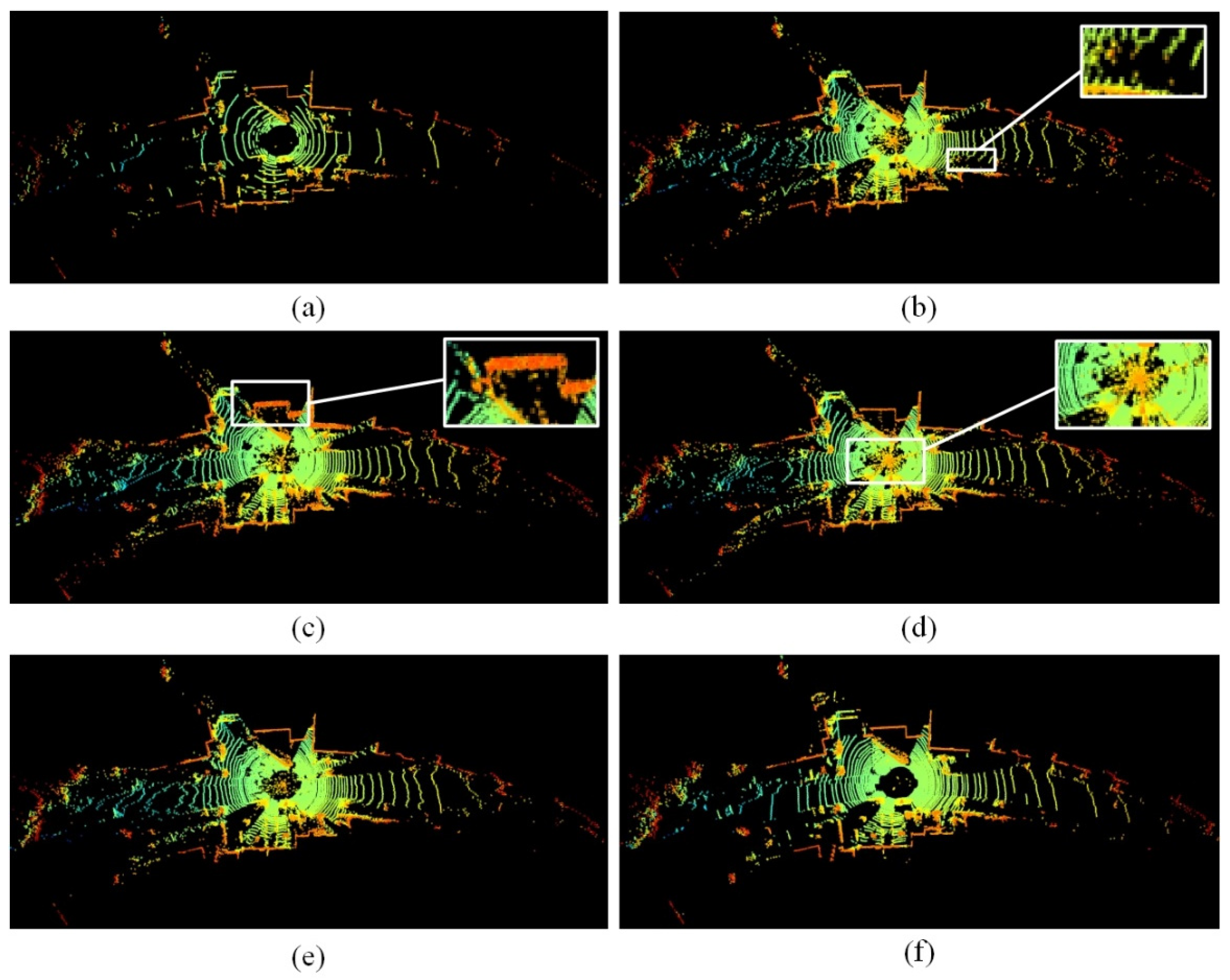
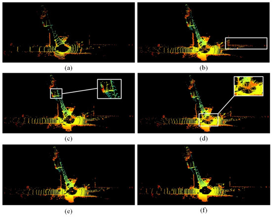
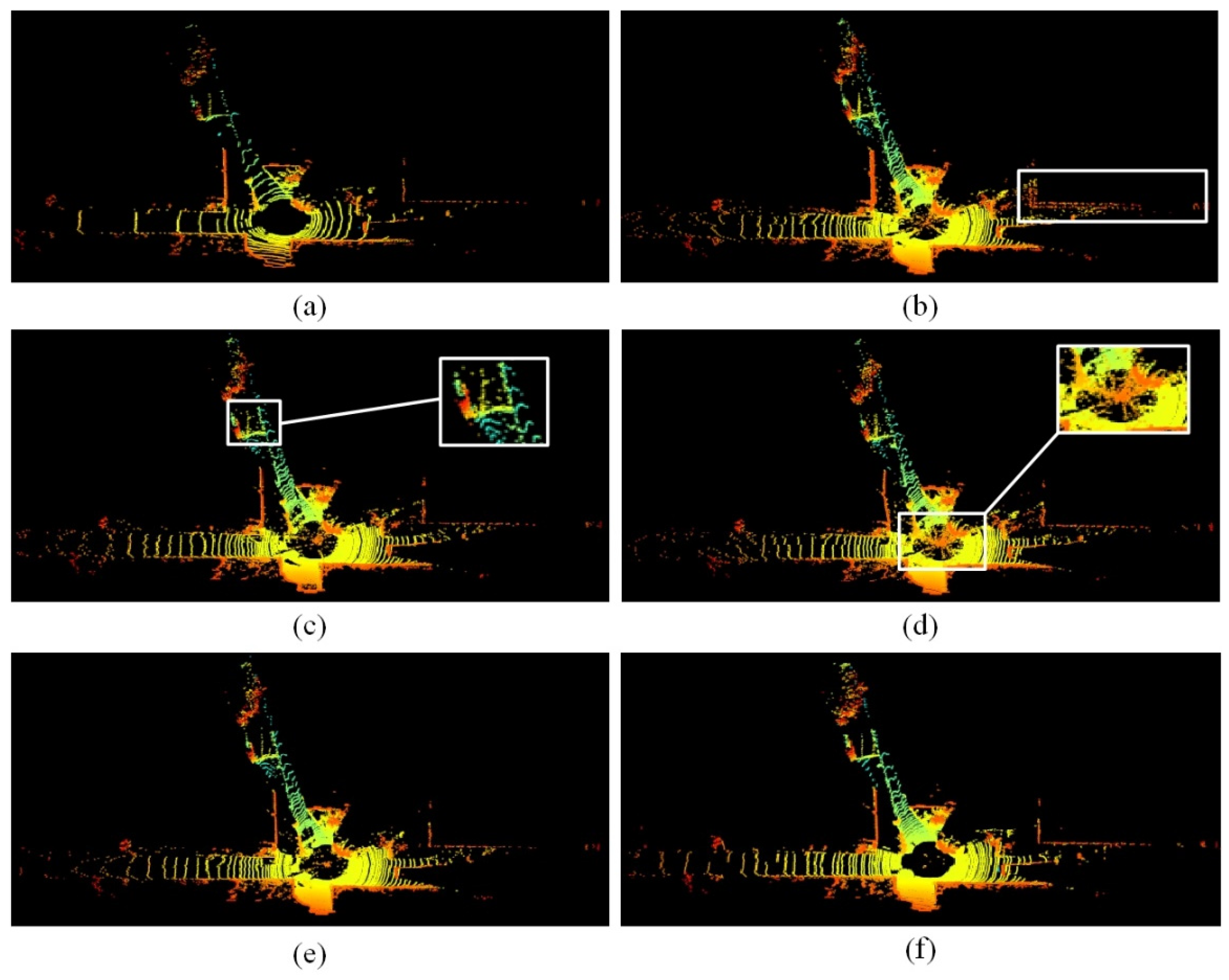
To intuitively verify the super-resolution effects, two typical scenes were selected from the KITTI test set to compare the reconstruction results of each method, as shown in Figure 5 and Figure 6. In large planar regions such as building façades, LIIF produces clearly over-smoothed point clouds, which weakens depth variations near planar boundaries and makes geometric boundaries less distinct. Although LiDAR-SR increases point cloud density, the point distribution over planar regions remains uneven, and local blur and structural discontinuities occur along object contours. TULIP recovers the overall scene outline relatively well, but isolated points and geometric artifacts remain near building edges and regions with abrupt depth changes. In contrast, the proposed method produces more continuous and planar surfaces with a more uniform point distribution, without evident local swelling or depressions. It also preserves clearer and more continuous geometric boundaries in depth-discontinuous regions such as road edges, thereby reducing boundary diffusion and excessive smoothing. In addition, the number of floating outliers is substantially reduced, indicating that the proposed uncertainty-guided height-adaptive filtering strategy effectively suppresses geometric artifacts caused by low-confidence predictions. Overall, the proposed method improves planar continuity, edge clarity, and local geometric integrity while increasing point cloud density, consistent with the quantitative results.

Figure 5. Super-resolution results on Sequence 09. (a) Input, (b) LIIF, (c) LiDAR-SR, (d) TULIP, (e) ours, (f) ground truth.

Figure 6. Super-resolution results on Sequence 10. (a) Input, (b) LIIF, (c) LiDAR-SR, (d) TULIP, (e) ours, (f) ground truth.

To verify the contribution of each core module in the proposed method, ablation experiments were conducted on the KITTI test set, and the results are shown in Table 4. In these experiments, W/o MDCF replaces the MDCF module with a standard 3 × 3 convolution having the same input and output channel dimensions; W/o motion compensation indicates that motion compensation is not performed; instead, consecutive multi-frame LiDAR point clouds are directly projected into range images and concatenated. W/o Anisotropy replaces the anisotropic Swin Transformer with a standard Swin Transformer encoder, W/o CASE uses standard feature concatenation for skip connections, and W/o adaptive filtering uses basic MC Dropout without the proposed adaptive filtering strategy. W/o structural loss removes the proposed structural consistency loss.

Table 4. Super-resolution performance results on the KITTI dataset.

Methods	MAE	IoU
W/o MDCF	0.5251	0.4423
W/o motion compensation	0.5012	0.4537
W/o Anisotropy	0.5711	0.4044
W/o CASE	0.5257	0.4137
W/o adaptive filtering	0.5363	0.4301
W/o structural loss	0.5064	0.4308
Ours	0.4916	0.4633

The ablation results show that the full model achieves the best performance in both MAE and IoU, indicating that all components contribute positively to the overall performance. Among them, the anisotropic Swin Transformer provides the largest contribution. Removing it causes the most substantial performance degradation, demonstrating that it effectively exploits the physical characteristics of LiDAR data and models long-range horizontal geometric dependencies, making it a key component for improving reconstruction performance. After removing the MDCF module, MAE increases from 0.4916 to 0.5251 and IoU decreases from 0.4633 to 0.4423, indicating that multi-frame temporal feature fusion effectively exploits complementary observations from adjacent frames and improves both range prediction accuracy and structural recovery. After removing ego-motion compensation, the MAE increases from 0.4916 to 0.5012, while the IoU decreases from 0.4633 to 0.4537. Although the performance degradation is moderate, the consistent deterioration in both metrics indicates that registering the preceding frames to the current reference frame can effectively reduce geometric inconsistencies caused by platform motion, providing a more reliable basis for subsequent multi-frame temporal fusion. After removing CASE, the decrease in IoU is more pronounced than the increase in MAE, suggesting that this module has a limited effect on point-wise range error but substantially improves local geometric details and overall structural integrity. Compared with basic MC Dropout, the proposed adaptive filtering strategy combines a height prior with a nonlinear adaptive threshold, enabling more accurate identification and suppression of low-confidence artifacts and further improving reconstruction quality. Finally, removing the structural consistency loss increases MAE by 3.0% and decreases IoU by 7.0%. This result indicates that the point-wise loss maintains basic range prediction accuracy but is insufficient to constrain local geometric relationships.

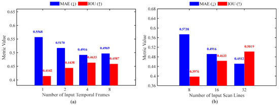
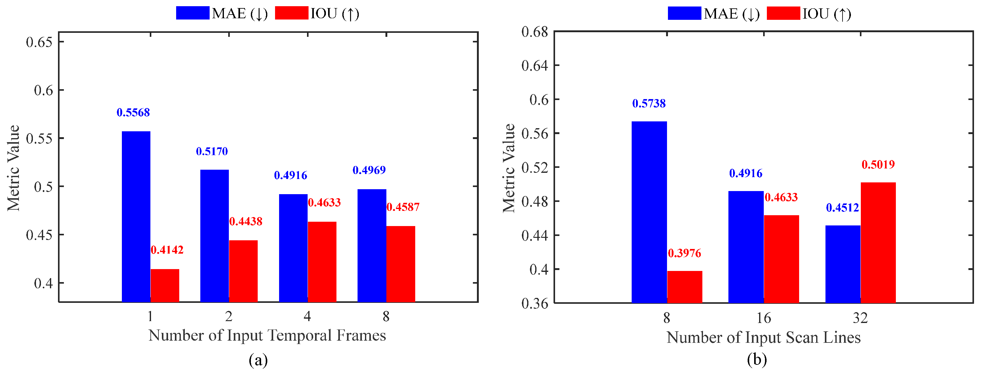
To further evaluate the adaptability of the proposed method to different input configurations, comparative experiments were conducted using different numbers of input temporal frames and different vertical scan-line resolutions. For the temporal-frame experiment, the number of input frames was set to 1, 2, 4, and 8. For the scan-line-resolution experiment, point clouds with 8, 16, and 32 scan lines were used as input, and the target output was a 64-line point cloud in all cases. Each configuration was trained independently, while the remaining network architecture, data split, and training parameters were kept unchanged. The results are shown in Figure 7.

Figure 7. Robustness of the proposed method to different input configurations. (a) Input temporal frames, (b) input scan lines.

As shown in Figure 7a, model performance improves as the number of input frames increases from 1 to 4. Compared with the single-frame setting, the four-frame setting reduces MAE from 0.5568 to 0.4916 and increases IoU from 0.4142 to 0.4633, corresponding to improvements of approximately 11.7% and 11.9%, respectively. These results indicate that multi-frame observations effectively compensate for the spatial sparsity of a single-frame point cloud and improve both range prediction accuracy and geometric recovery. When the number of frames is further increased to 8, both MAE and IoU deteriorate slightly, suggesting that the benefit of temporal information tends to saturate near four frames and may be affected by redundant observations over a longer temporal window. As shown in Figure 7b, model performance improves steadily as the number of input scan lines increases. Increasing the input from 8 to 16 scan lines improves MAE and IoU by 14.3% and 16.5%, respectively. A further increase from 16 to 32 scan lines yields additional improvements of 8.2% and 8.3%. These results indicate that a higher vertical scan-line resolution provides more complete geometric observations and reduces the difficulty of super-resolution reconstruction. The stable performance trend across different input resolutions also demonstrates that the proposed method can adapt to point clouds with different degrees of sparsity.

To verify whether the performance improvement of the proposed method mainly results from the use of multi-frame inputs, we conducted a multi-frame comparison experiment. Specifically, while keeping the original backbone architectures and other training hyperparameters unchanged, the inputs of LiDAR-SR and TULIP were extended to four consecutive range images. As shown in Table 5, introducing multi-frame observations improves the reconstruction performance of both baselines, indicating that additional temporal information itself is beneficial for LiDAR super-resolution. When the number of input frames for LiDAR-SR is increased from one to four, the MAE decreases from 0.5720 to 0.5368, while the IoU increases from 0.4101 to 0.4327. Similarly, for the four-frame TULIP variant, the MAE decreases from 0.5321 to 0.5076, and the IoU increases from 0.4112 to 0.4398. However, under the same four-frame input setting, the proposed method still achieves the lowest MAE (0.4916) and the highest IoU (0.4633). Compared with the four-frame TULIP variant, the proposed method further reduces the MAE by approximately 3.2% and improves the IoU by approximately 5.3%. These results demonstrate that, under the same temporal input conditions, the temporal fusion and structural modeling mechanisms of the proposed method can make more effective use of multi-frame observations, thereby achieving better reconstruction accuracy.

Table 5. Comparison under single-frame and matched four-frame input settings.

Method	Input Frames	MAE	IoU
LiDAR-SR	1	0.5720	0.4101
LiDAR-SR	4	0.5368	0.4327
TULIP	1	0.5321	0.4112
TULIP	4	0.5076	0.4398
Ours	1	0.5568	0.4142
Ours	4	0.4916	0.4633

To verify the impact of super-resolution results on downstream SLAM performance, experiments were conducted on sequences 09 and 10. The original low-resolution point clouds and the super-resolution point clouds from each method were separately fed into A-LOAM, and the RPE results are shown in Table 6.

Table 6. RPE results on the KITTI dataset.

Seq.	Methods	RTE (%)	RRE (deg/100 m)
09	Raw point cloud	1.91	0.79
	LIIF	1.99	0.81
	LiDAR-SR	1.65	0.68
	TULIP	1.41	0.66
	Ours	1.18	0.53
10	Raw point cloud	2.48	1.39
	LIIF	2.67	1.66
	LiDAR-SR	2.23	1.15
	TULIP	2.07	1.10
	Ours	1.71	0.98

The results indicate that not all super-resolution methods improve SLAM accuracy. For example, after inputting the point clouds processed by LIIF into A-LOAM, the localization accuracy was slightly lower than that of the original low-resolution point clouds. This suggests that while increasing point cloud density, the method blurred key geometric features in the original point clouds, interfering with the feature matching process and leading to increased pose estimation errors. Although LiDAR-SR and TULIP bring certain improvements, their performance gains are still limited. In contrast, the proposed method achieves the most significant performance improvement. Compared with the original low-resolution point clouds, the point clouds reconstructed by the proposed method reduce RTE and RRE by 38.2% and 32.9%, respectively, on Sequence 09. On Sequence 10, the two errors are reduced by approximately 31.0% and 29.5%, respectively. These improvements mainly arise from the method’s emphasis on structural consistency, which produces clearer and more stable edge and planar features and therefore provides more reliable geometric constraints for feature matching and pose estimation in SLAM.

4.3. Validation on the Self-Collected Dataset

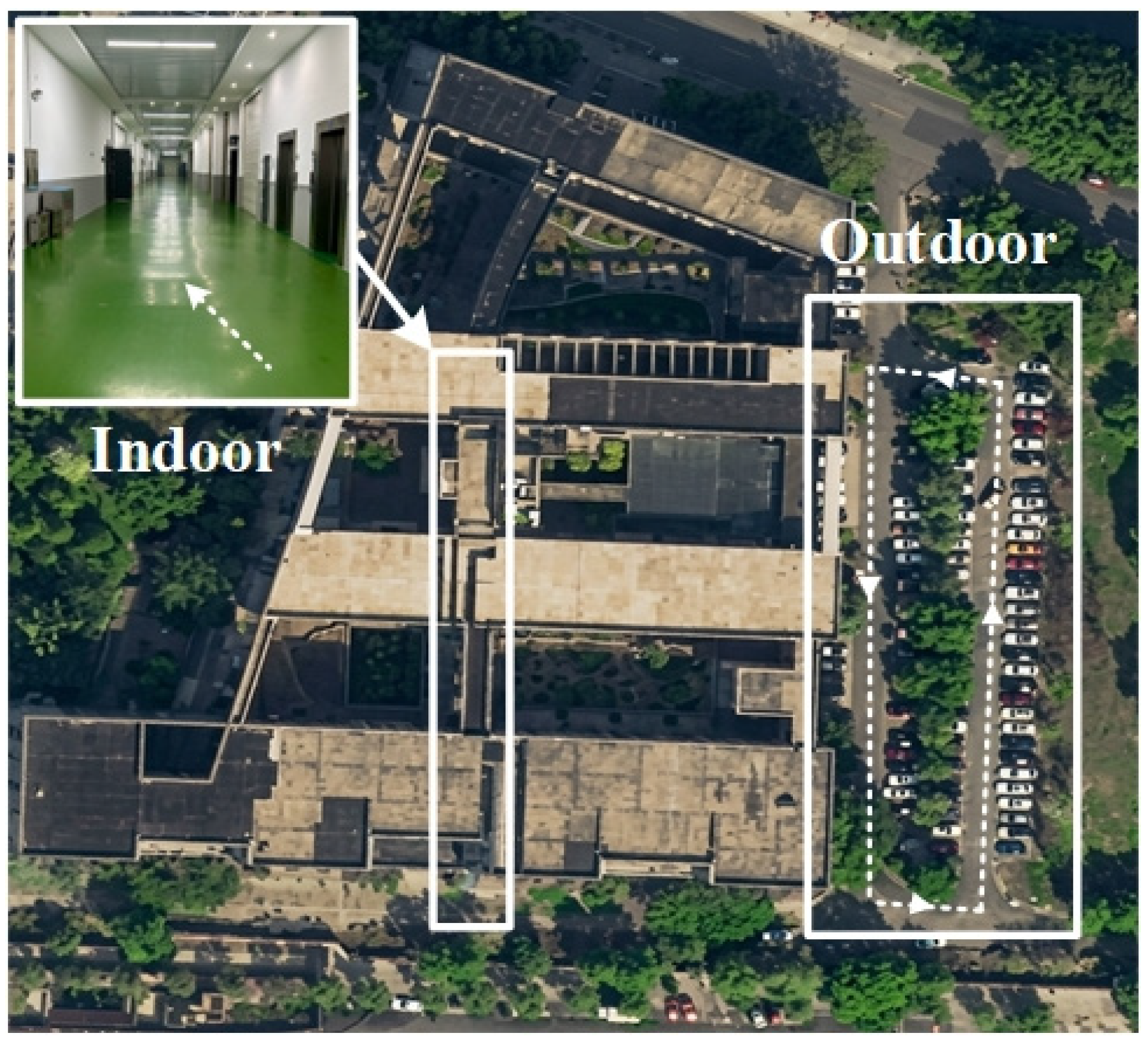
To further evaluate the applicability of the proposed method under different sensor and scene conditions, tests were conducted on the self-collected CSU-SLAM dataset. As shown in Figure 8, this dataset consists of two sequences: an indoor corridor sequence and an outdoor open campus sequence. The indoor sequence was collected in a long corridor within a teaching building, characterized by simple geometric structures and significant scene degeneration. The outdoor sequence was collected in campus squares and road areas, containing diverse structures such as trees and buildings. The key statistics of the two sequences are listed in Table 7. It should be noted that no global ground-truth trajectory is available for the indoor corridor sequence because GNSS signals are unavailable indoors. During data collection, the robot was controlled to return to the starting point of a closed loop so that the physical start and end positions coincided. Therefore, the endpoint position error (EPE), defined as the Euclidean distance between the estimated start and end positions, is used as an endpoint loop-consistency metric for this sequence.

Figure 8. CSU-SLAM dataset collection scenario.

Table 7. Key statistics of the two test sequences.

Sequence	Trajectory Length	Number of Frames	Reference Trajectory Source
Indoor	86 m	1720	Closed-loop endpoint error
Outdoor	210 m	4200	RTK

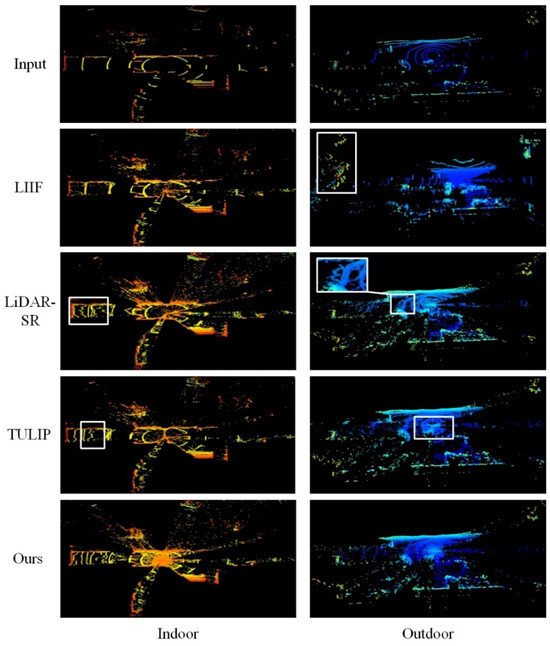
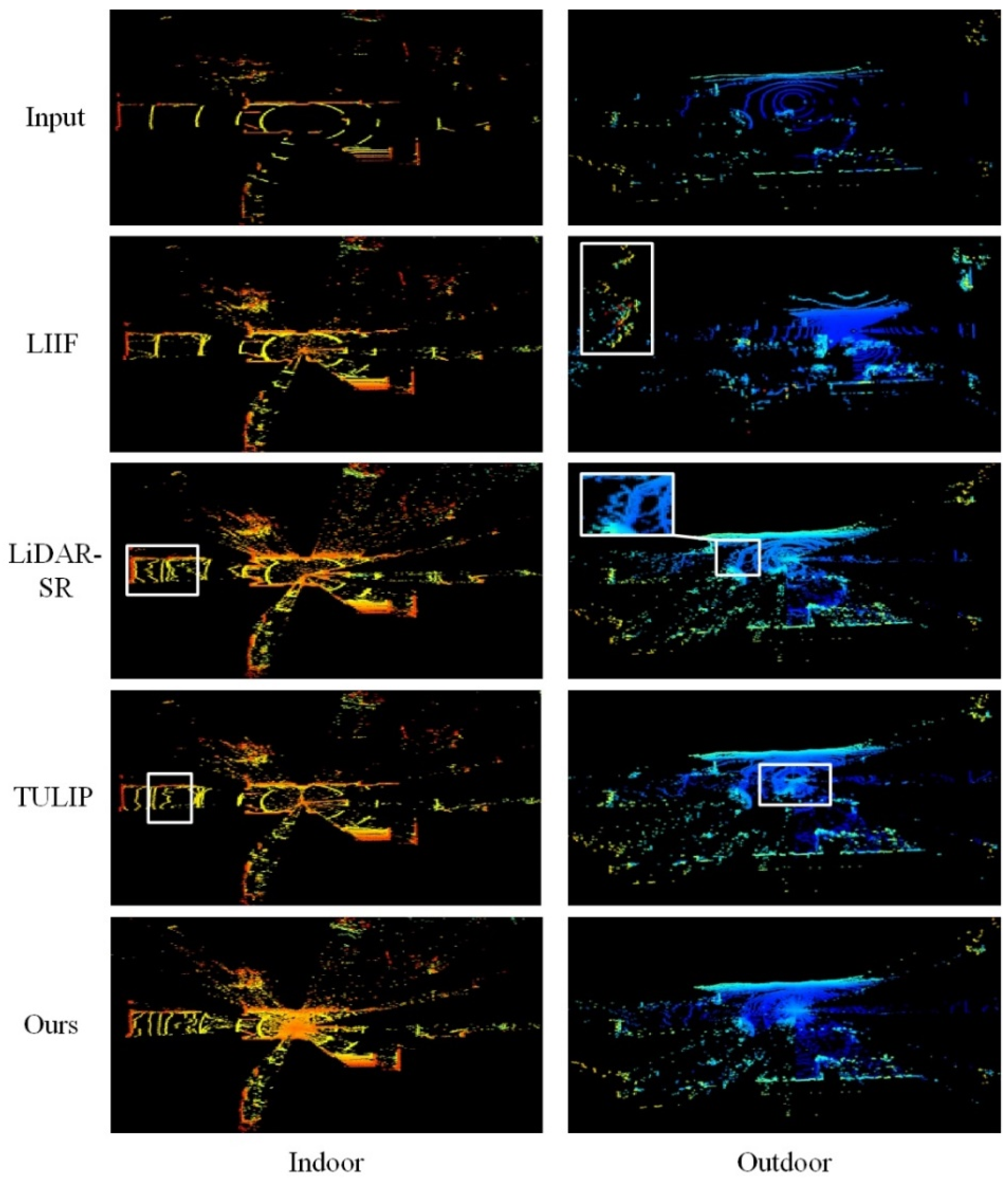
Because the self-collected dataset does not provide corresponding high-resolution point cloud ground truth, MAE and IoU cannot be calculated. Therefore, the reconstruction quality of the different methods under the new sensor configuration was evaluated qualitatively. Figure 9 shows representative super-resolution results. In the indoor corridor scene, although LiDAR-SR and TULIP increase point cloud density, numerous outliers remain near wall–floor intersections, the longitudinal corridor boundaries exhibit local blur and discontinuities, and the distant structures show a certain degree of deformation. In contrast, the proposed method reconstructs flatter wall and floor surfaces, preserves better linearity and continuity along the corridor contours, produces clearer wall–floor intersections, and avoids evident structural distortion or duplicated artifacts in distant regions. These observations indicate stable structural recovery in indoor environments with sparse geometric features. In the outdoor campus scene, LIIF produces evident over-smoothing near building edges and object boundaries, whereas LiDAR-SR and TULIP still exhibit local swelling, boundary diffusion, and clustered noise, resulting in damaged building contours and road boundaries. In contrast, the proposed method reconstructs flatter building façades, preserves clearer and more continuous geometric boundaries at building corners and road edges and between trees and the background, and avoids evident spurious structures, further indicating its potential applicability across different scenes and sensor configurations.

Figure 9. Super-resolution results on the CSU-SLAM dataset.

To evaluate the application effectiveness of the super-resolved point clouds in real-world scenarios, the reconstruction results of each method were similarly input into the A-LOAM framework for SLAM testing, with the localization accuracy results summarized in Table 8. When the point clouds generated by LiDAR-SR and LIIF are used for SLAM, the localization accuracy is slightly lower than that obtained using the original low-resolution point clouds. This is because these methods increase point cloud resolution while disrupting a limited number of reliable geometric features in the original point clouds. TULIP improves localization performance, but the improvement remains limited, particularly in indoor scenes with sparse geometric features. This indicates that methods designed primarily for high reconstruction accuracy may still generate geometric structures that deviate from the features required by the SLAM system, making it difficult to translate reconstruction quality into effective localization constraints. In contrast, the proposed method yields the most substantial and stable improvement. For the indoor corridor sequence, EPE is reduced by 24.0% relative to the original point cloud. For the outdoor campus sequence, RTE and RRE values are reduced by 23.9% and 25.0%, respectively. These improvements mainly result from the effective preservation of structural consistency during reconstruction, which produces clearer and more reliable edge and planar features and thereby improves feature matching and pose estimation in SLAM.

Table 8. SLAM performance on the CSU-SLAM dataset.

Methods	Indoor	Outdoor
	EPE (m)	RTE (%)	RRE (deg/100 m)
Initial point cloud	2.25	2.17	0.84
LIIF	2.41	2.31	0.89
LiDAR-SR	2.29	2.19	0.91
TULIP	1.94	1.84	0.77
Ours	1.71	1.65	0.63

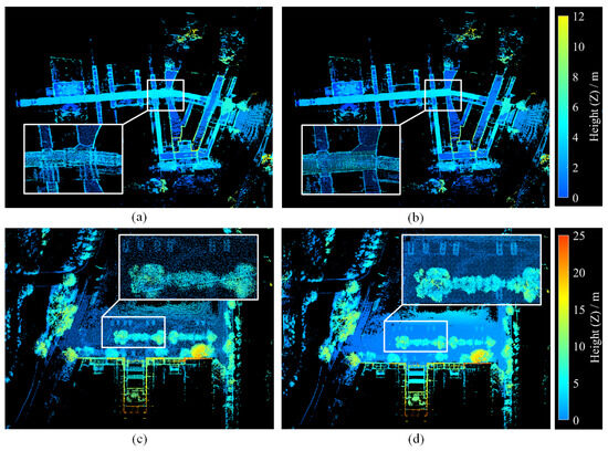
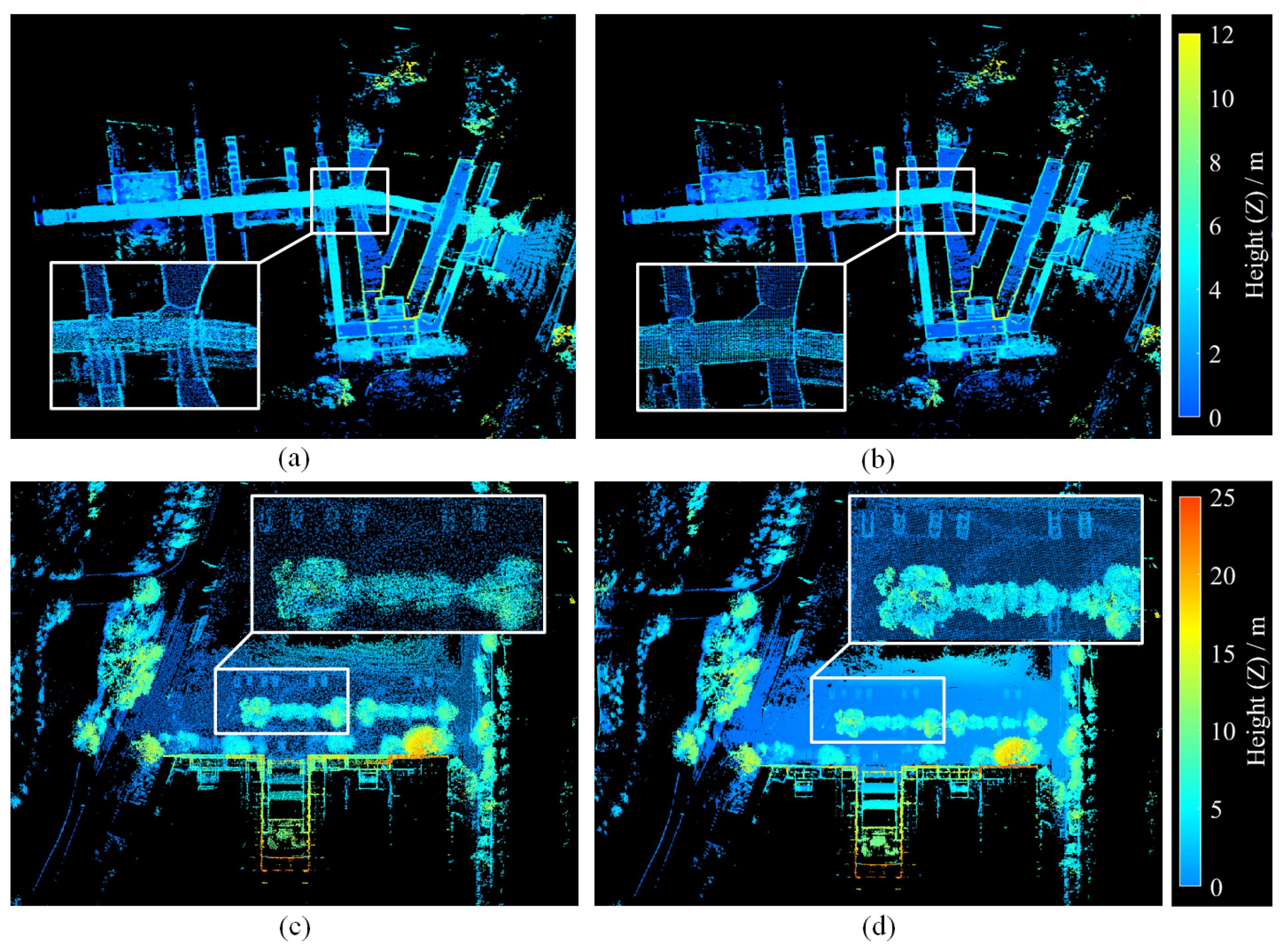
The mapping results in Figure 10 further demonstrate the advantage of the proposed method. In the indoor corridor scene, the robot is prone to pose drift when passing through geometrically critical regions such as corridor corners because of the insufficient geometric constraints in the original low-resolution point clouds, thereby reducing local map consistency. With the point clouds reconstructed by the proposed method, the walls on both sides of the corridor maintain good parallelism, wall thickness is more uniform, and wall–corner connections are more continuous, without evident duplicated contours or local misalignment, resulting in higher map quality. In the outdoor campus scene, the map generated by the proposed method better preserves the flatness of building façades, while building corners, road boundaries, and the contours of static objects are clearer and more complete. These results further demonstrate the effectiveness of the proposed method for downstream SLAM mapping.

Figure 10. Mapping results on the CSU-SLAM dataset. (a) Indoor mapping using the raw point cloud, (b) indoor mapping using the super-resolved point cloud, (c) outdoor mapping using the raw point cloud, and (d) outdoor mapping using the super-resolved point cloud.

To evaluate the online processing capability of the proposed method, the computational efficiency of different super-resolution methods was further tested, as reported in Table 9. Specifically, model inference refers only to the forward inference time of the super-resolution network, whereas per-frame processing refers to the online processing time from the low-resolution input to the high-resolution point-cloud output, followed by single-frame pose estimation using A-LOAM. Compared with LIIF, LiDAR-SR, and TULIP, the proposed method incurs additional computational overhead because it performs multi-frame temporal feature fusion, 10 MC Dropout forward passes, and adaptive filtering during inference. Its average per-frame processing time is 88.4 ms, corresponding to an average processing frequency of 11.3 Hz. Although its processing efficiency is slightly lower than that of the comparison methods, it still satisfies the online processing requirement of a 10 Hz LiDAR. The proposed method therefore achieves a practical balance among point cloud super-resolution quality, SLAM localization accuracy, and computational efficiency while maintaining online operation.

Table 9. Computational efficiency comparison of different super-resolution methods.

Method	Model Inference	Per-Frame Processing	Processing Frequency
LIIF	46.2 ms	71.8 ms	13.9 Hz
LiDAR-SR	18.7 ms	44.1 ms	22.7 Hz
TULIP	31.5 ms	57.0 ms	17.5 Hz
Ours	61.8 ms	88.4 ms	11.3 Hz

5. Conclusions

To address the problem that existing LiDAR super-resolution methods struggle to effectively preserve structural consistency during reconstruction, this paper proposes a structural consistency-aware LiDAR super-resolution method. By integrating the MDCF module, an anisotropic Swin Transformer, the CASE module, and uncertainty-guided height-adaptive filtering, the proposed method effectively improves the geometric integrity and structural reliability of high-resolution point clouds. Meanwhile, a structural consistency loss function based on local curvature is designed, enabling the network to explicitly focus on and preserve the clarity and completeness of key geometric features, such as edges and planes, during the reconstruction process. Experimental results on the KITTI public dataset and the self-collected CSU-SLAM dataset demonstrate that the proposed method outperforms existing mainstream methods in core super-resolution metrics such as MAE and IoU, and is capable of generating high-resolution point clouds with clear structures and high geometric reliability. When the reconstructed point clouds are applied to A-LOAM, a classic LiDAR SLAM framework, the RPE values are significantly reduced. The proposed method exhibits favorable localization and mapping performance in both indoor degenerate scenes and complex outdoor environments, validating its positive effect on downstream tasks while improving the geometric quality of point clouds.

Nevertheless, the proposed method still has several limitations, including relatively high computational overhead and limited adaptability to dynamic scenes and cross-sensor settings. In addition, because the CSU-SLAM dataset lacks dense ground truth and the downstream evaluation was conducted only with A-LOAM, the general applicability of the method requires further validation. Future work will focus on improving real-time performance, robustness, and cross-scene generalization, together with broader evaluation in practical applications.

References

- Wang, Z.; Tang, X.; Zhou, H.; Xiao, L.; Duan, J. 3D LiDAR SLAM for natural guided navigation of automated guided vehicles in unstructured scenes. Meas. Sci. Technol. 2025, 36, 026317. [Google Scholar] [CrossRef] [Scilit]
- Yue, J.; Wen, W.; Han, J.; Hsu, L.-T. 3D Point Clouds Data Super Resolution-Aided LiDAR Odometry for Vehicular Positioning in Urban Canyons. IEEE Trans. Veh. Technol. 2021, 70, 4098–4112. [Google Scholar] [CrossRef] [Scilit]
- Cheng, X.; Wu, L.; Wang, Z.; Hou, J.; Wen, J.; Xu, Y. PVNet: Point–Voxel Interaction LiDAR Scene Upsampling via Diffusion Models. IEEE Trans. Image Process. 2025, 34, 6895–6910. [Google Scholar] [CrossRef] [Scilit] [PubMed]
- Zhang, C.; Long, C.; Xu, H.; Zhang, W.; Dong, Z.; Yang, B. WIN: Variable-View Implicit LiDAR Upsampling Network. IEEE Trans. Intell. Transp. Syst. 2025, 26, 19347–19359. [Google Scholar] [CrossRef] [Scilit]
- Chen, C.; Lin, Y.; Hu, J.; Yuan, X.; Ge, W. SRMambaV2: Bioinspired Attention for Sparse Point Cloud Upsampling in Autonomous Driving. IEEE Sens. J. 2026, 26, 2431–2442. [Google Scholar] [CrossRef] [Scilit]
- Chen, X.; Läbe, T.; Milioto, A.; Röhling, T.; Behley, J.; Stachniss, C. OverlapNet: A Siamese Network for Computing LiDAR Scan Similarity with Applications to Loop Closing and Localization. Auton. Robot. 2022, 46, 61–81. [Google Scholar] [CrossRef] [Scilit]
- Kwon, Y.; Sung, M.; Yoon, S.-E. Implicit LiDAR Network: LiDAR Super-Resolution via Interpolation Weight Prediction. In Proceedings of the 2022 IEEE International Conference on Robotics and Automation (ICRA), Philadelphia, PA, USA, 23–27 May 2022; pp. 8424–8430. [Google Scholar] [CrossRef] [Scilit]
- Yang, B.; Pfreundschuh, P.; Siegwart, R.; Hutter, M.; Moghadam, P.; Patil, V. TULIP: Transformer for Upsampling of LiDAR Point Clouds. In Proceedings of the 2024 IEEE/CVF Conference on Computer Vision and Pattern Recognition (CVPR), Seattle, WA, USA, 16–22 June 2024; pp. 15354–15364. [Google Scholar] [CrossRef] [Scilit]
- Gkillas, A.; Lalos, A.S.; Markakis, E.K.; Politis, I. A Federated Deep Unrolling Method for LiDAR Super-Resolution: Benefits in SLAM. IEEE Trans. Intell. Veh. 2024, 9, 199–215. [Google Scholar] [CrossRef] [Scilit]
- Wang, Z.; Zhou, H.; Duan, J. DALO-SLAM: LiDAR-Only SLAM Based on Dynamic Removal and Adaptive Feature Enhancement in GNSS-Denial Environment. Meas. Sci. Technol. 2025, 36, 066316. [Google Scholar] [CrossRef] [Scilit]
- Chen, Y.; Liu, S.; Wang, X. Learning Continuous Image Representation with Local Implicit Image Function. In Proceedings of the 2021 IEEE/CVF Conference on Computer Vision and Pattern Recognition (CVPR), Nashville, TN, USA, 20–25 June 2021; pp. 8624–8634. [Google Scholar] [CrossRef] [Scilit]
- Park, M.; Son, H.; Kim, E. Implicit Point Function for LiDAR Super-Resolution in Autonomous Driving. IEEE Robot. Autom. Lett. 2023, 8, 7003–7009. [Google Scholar] [CrossRef] [Scilit]
- Zhao, W.; Liu, X.; Zhong, Z.; Jiang, J.; Gao, W.; Li, G.; Ji, X. Self-Supervised Arbitrary-Scale Point Clouds Upsampling via Implicit Neural Representation. In Proceedings of the 2022 IEEE/CVF Conference on Computer Vision and Pattern Recognition (CVPR), New Orleans, LA, USA, 19–24 June 2022; pp. 1989–1997. [Google Scholar] [CrossRef] [Scilit]
- Chen, C.; Jin, A.; Wang, Z.; Zheng, Y.; Yang, B.; Zhou, J.; Xu, Y.; Tu, Z. SGSR-Net: Structure Semantics Guided LiDAR Super-Resolution Network for Indoor LiDAR SLAM. IEEE Trans. Multimed. 2024, 26, 1842–1854. [Google Scholar] [CrossRef] [Scilit]
- Triess, L.T.; Peter, D.; Rist, C.B.; Enzweiler, M.; Zöllner, J.M. CNN-Based Synthesis of Realistic High-Resolution LiDAR Data. In Proceedings of the 2019 IEEE Intelligent Vehicles Symposium (IV), Paris, France, 9–12 June 2019; pp. 1512–1519. [Google Scholar] [CrossRef] [Scilit]
- Shan, T.; Wang, J.; Chen, F.; Szenher, P.; Englot, B. Simulation-Based LiDAR Super-Resolution for Ground Vehicles. Robot. Auton. Syst. 2020, 134, 103647. [Google Scholar] [CrossRef] [Scilit]
- Chen, K.; Liu, C.; Ou, Y. Channel Attention Based Network for LiDAR Super-Resolution. In Proceedings of the 2021 China Automation Congress (CAC), Beijing, China, 22–24 October 2021; pp. 5458–5463. [Google Scholar] [CrossRef] [Scilit]
- Tian, D.; Zhao, D.; Cheng, D.; Zhang, J. LiDAR Super-Resolution Based on Segmentation and Geometric Analysis. IEEE Trans. Instrum. Meas. 2022, 71, 8504917. [Google Scholar] [CrossRef] [Scilit]
- Jung, Y.; Seo, S.-W.; Kim, S.-W. Fast Point Clouds Upsampling with Uncertainty Quantification for Autonomous Vehicles. In Proceedings of the 2022 IEEE International Conference on Robotics and Automation (ICRA), Philadelphia, PA, USA, 23–27 May 2022; pp. 7776–7782. [Google Scholar] [CrossRef] [Scilit]
- Ren, L.; Li, D.; Ouyang, Z.; Zhang, Z. TSE-UNet: Temporal and Spatial Feature-Enhanced Point Cloud Super-Resolution Model for Mechanical LiDAR. Appl. Sci. 2024, 14, 1510. [Google Scholar] [CrossRef] [Scilit]
- Zhang, J.; Singh, S. LOAM: LiDAR Odometry and Mapping in Real-Time. In Proceedings of the Robotics: Science and Systems X, Berkeley, CA, USA, 12–16 July 2014; pp. 1–9. [Google Scholar] [CrossRef] [Scilit]
- Geiger, A.; Lenz, P.; Urtasun, R. Are We Ready for Autonomous Driving? The KITTI Vision Benchmark Suite. In Proceedings of the 2012 IEEE Conference on Computer Vision and Pattern Recognition (CVPR), Providence, RI, USA, 16–21 June 2012; pp. 3354–3361. [Google Scholar] [CrossRef]
Disclaimer/Publisher’s Note: The statements, opinions and data contained in all publications are solely those of the individual author(s) and contributor(s) and not of MDPI and/or the editor(s). MDPI and/or the editor(s) disclaim responsibility for any injury to people or property resulting from any ideas, methods, instructions or products referred to in the content. |
© 2026 by the authors. Licensee MDPI, Basel, Switzerland. This article is an open access article distributed under the terms and conditions of the Creative Commons Attribution (CC BY) license.