Signal-Feature-Matched Non-Uniform Photonic Sampling and Broadband Waveform Reconstruction

Abstract

This paper proposes Non-Uniform Adaptive Acquisition (NUAA), a signal-feature-matched non-uniform adaptive photonic sampling framework that recovers broadband radio-frequency (RF) waveforms from highly sparse programmable non-uniform photonic sampling points. A 200 MHz mode-locked laser together with five electrical optical delay lines (EDLs; motor-actuated optical delay units) arranges the non-uniform sampling instants. Benefiting from the joint design of the photodetector/track-and-hold amplifier (PD/THA) response model and programmable non-uniform optical pulse spacing, a low-bandwidth PD infers neighboring pulse amplitudes from their deterministic superposition at the readout. In numerical simulations of this physical forward operator, that construction corresponds to a 1 THz equivalent sampling rate on the 1 ps EDL grid, while the electrical front end operates at a 1 GHz average sampling rate (cascaded PD–THA analog 3 dB bandwidth $\approx 0.676$ GHz). Under severe blocking interference and low signal-to-noise ratio (SNR), the numerical simulations show that the strongest broadband chirplet result uses a scene prior with support locking: with the NUAA–MU (Mamba–Unfolding) reconstructor at 0.1% multi-coset sparsity, all $N_{\mathrm{trial}}=50$ Monte Carlo trials succeed within 200 ms (Wilson 95% CI $[93, 100]\%$; cumulative-best NMSE $-28.0$ dB), whereas the configuration without a scene prior is substantially weaker in the same window. A scene prior may come from known radar or communication waveform families, coarse occupancy reported by a companion sensor, or accumulation across related tasks.

1. Introduction

Microwave photonics exploits the large bandwidth, low loss, and immunity to electromagnetic interference of optical waves to move broadband RF processing functions into the optical domain, enabling instantaneous bandwidth observation at tens of GHz and beyond [1,2,3,4,5]. The reception objective is nevertheless shifting from sparse spectrum estimation to dynamic waveform recovery: under strong interference, low SNR, and non-ideal readout, a system must reconstruct waveforms or parameter trajectories for radar, communication, and cognitive electronic warfare [2,6].

Current research on photonic analog-to-digital converters (ADCs) concentrates on optical sampling combined with electronic quantization schemes [3,7,8]. Although optical pulses can significantly reduce sampling aperture jitter, almost all practical systems still require complete electronic ADC backends, and are therefore inevitably affected by ENOB, clock, channel mismatch, and calibration issues [7,8]. Photonic spectrum sensing and compressive receivers based on classical compressive sensing (CS) theory further exploit optical-domain mixing and sparse priors to lower the backend sampling rate [4,5], but the equivalent sampling rate is still constrained by the bandwidth of the pseudo-random waveform generator, and most implementations terminate at sparse spectrum estimation rather than broadband waveform inversion.

Periodic non-uniform sampling, multi-coset sampling, and Xampling theory [9,10,11] show that multi-band signals can be recovered at an average sampling rate far below twice the highest frequency, but successful recovery depends on support sparsity, the rank of the measurement matrix, and the size of the candidate set [11]. Learning-based compressed sensing [12,13] further shows that the sampling matrix and the reconstruction network can be jointly optimized, but hardware constraints often determine which matrices can be realized [12].

In parallel, recent work on irregular time series has moved beyond uniform-grid assumptions. Continuous-time Transformers such as ContiFormer embed Neural-ODE dynamics into attention [14]. Sample-centric encoders such as CoFormer handle asynchronous multivariate observations without imputation [15]. Latent stochastic differential equations (SDEs) model sparse irregular trajectories for anomaly detection without resampling [16]. Concurrently, selective state-space models (SSMs), culminating in Mamba [17], have revived linear-time recurrence for long sequences [18], with bidirectional Mamba blocks used for multivariate imputation (TIMBA) [19] and long-term forecasting [20,21]; unrolled Mamba reconstructors have also been explored for inverse problems [22]. A remaining gap is to embed multi-coset mathematics, compressed-sensing reconstruction, SSM-style sequence priors, and signal feature information [9,10,11,17,22,23,24] inside a microwave photonic front end with band-limited PD readout.

Against this backdrop, this paper proposes Non-Uniform Adaptive Acquisition (NUAA), an adaptive microwave photonic analog-to-information (A2I) conversion framework [10,25,26] that jointly designs the photonic sampling layout and the digital recovery path. The photonic front end continuously outputs non-uniform sampling points at a low average sampling rate. The digital backend jointly (i) optimizes the temporal sampling-pulse pattern (EDL/strobe commands), (ii) pretrains and online-accumulates signal feature priors, and (iii) reconstructs the broadband waveform under a physically consistent forward operator. The EDLs provide a tuning precision of $\eta =1$ ps, which sets the equivalent sampling rate on that grid to $f_{\mathrm{eq},\mathrm{Nyq}}=1/\eta =1$ THz. Five programmable time slots within every 5 ns master period are activated, forming a multi-coset sampling point stream with 0.1% sparsity. NUAA achieves de-aliasing through cross-window accumulation, feature priors, and physically consistent inversion. Benefiting from the joint design of a PD response model and programmable non-uniform optical pulse spacing, a low-bandwidth PD can infer neighboring pulse amplitudes from deterministic superposition at the readout. In the numerical simulations of this paper, that construction corresponds to a 1 THz equivalent sampling rate while the average electrical sampling rate remains $f_{\mathrm{avg}}=1\mathrm{GHz}$ and the cascaded PD–THA analog 3 dB bandwidth is $f_{\mathrm{PD}\text{-}\mathrm{THA}}\approx 0.676\mathrm{GHz}$. Reconstruction inverts the same operator $A\left(\tau \right)$ that the photonic layout produces.

The contributions of this paper can be summarized into three aspects:

• A non-uniform sampling model based on cascaded prefix-sum delay lines. This paper translates the measurement matrix into the prefix-sum codeword $\tau$ of five cascaded electrical optical delay lines, explicitly accounting for the bang–bang actuation rate (the delay only toggles between being stationary and shifting at the constant rate) and 1 ps time slots (determined by the tuning precision of the EDLs). This model is the foundation of NUAA’s sampling front end and of pattern control under that rate constraint.
• A band-limited PD/THA pulse-superposition forward model with strobe readout. Conventional photonic ADC practice treats electronic back-end bandwidth as a hard envelope that must remain comparable to the RF content of interest; once the RF support exceeds that envelope, the electrical output aliases and subsequent processing is impaired [7,8]. NUAA instead retains the linear PD/THA kernels inside $A\left(\tau \right)$ and uses programmable optical-pulse spacing so that neighboring pulses produce a known superposition at a low-bandwidth PD. Because photocurrent scales with optical power, the overlapped responses remain invertible when the layout and strobe are controlled precisely, corresponding in the present simulations to equivalent 1 THz sampling with a ∼1 GHz electrical front end.
• A feature-matched joint acquisition and reconstruction strategy. Prior photonic CS/A2I receivers predominantly target sparse spectrum estimation [4,5,10,26]. NUAA combines measurement diversity, interference-subspace handling, online belief/prior accumulation, evolution prediction, and the NUAA-MU reconstructor so that layout commands, priors, and inversion share the operator $A\left(\tau \right)$ and recover a broadband waveform.

2. System Architecture and Physical Model

2.1. Non-Uniform Photonic Sampling Front End

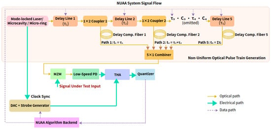
The NUAA front end is shown in Figure 1. A mode-locked laser or a microcavity optical frequency comb generates 200 MHz uniform optical pulses, with master period

$$T_0=5\mathrm{ns}.$$

(1)

Figure 1. Signal flow of the simulated NUAA non-uniform photonic sampling front end. A 200 MHz optical pulse train is split into five prefix-sum EDL branches, intensity-modulated by the RF input through an MZM, detected by a band-limited PD, and read out by a strobe-triggered THA and pure quantizer.

Five stages of electrical optical delay lines (EDLs)—motor-actuated optical delay units that set optical path length by electromechanical translation—are cascaded through $1\times 2$ optical fiber couplers. They form five prefix-sum delay branches:

$$t_l={\displaystyle \sum _{i=1}^l}{\tau }_i,l=1,\dots ,5,$$

(2)

where each stage delay ${\tau }_i\in [0, 1000)$ ps is an EDL codeword, with tuning precision $\eta =1$ ps, corresponding to a 1 THz equivalent sampling rate. The number of equivalent time slots within each master period is

$$N_0=T_0/\eta =5000.$$

(3)

After combining the five branches, the average sampling rate is

$$f_{\mathrm{avg}}=5/T_0=1\mathrm{GHz}.$$

(4)

Throughout this paper, $f_{\mathrm{avg}}$ denotes the mean photonic sampling rate, whereas $f_{\mathrm{PD}}$, $f_{\mathrm{THA}}$, and the cascaded readout bandwidth $f_{\mathrm{PD}\text{-}\mathrm{THA}}$ in Section 2.3 are analog 3 dB bandwidths of the electrical components. The core of NUAA is therefore to perform extremely sparse sampling at 1 ps-programmable instants, and then to use feature priors to achieve de-aliased recovery.

2.2. THA Strobe and Pure-Quantizer Readout

The combined non-uniform optical pulses are intensity-modulated by the RF signal under test via an MZM. Limited by the finite impulse response of the 1 GHz-bandwidth PD, adjacent photonic sampling pulses undergo deterministic linear superposition at the detection end. Direct sampling of the PD output with a high-speed ADC on a uniform clock would require raising both the sampling rate and the frontend analog bandwidth, and would reintroduce aperture jitter and ENOB degradation. NUAA therefore separates when to sample from how to digitize: a strobe-triggered track-and-hold amplifier (THA) captures the PD peak, and a pure quantizer converts only the held level into digital codes for the reconstruction algorithm.

In this paper, “pure quantizer” denotes the memoryless amplitude-quantization stage applied to the THA output voltage. Sampling timing is supplied by the programmable strobe and THA; ${\mathcal{Q}}_B$ does not define or require a uniform sampling clock, but acts on each non-uniformly timed, quasi-static held level. The resulting digital codes enter the digital backend. Concretely, the readout chain executes:

• The digital backend predicts the PD peak instant $t_i^{\mathrm{smp}}$ of each sampling point from the layout $\tau$ and the calibrated $H_{\mathrm{PD}}/H_{\mathrm{THA}}$ cascade.
• A DAC-generated strobe of nominal width equal to one equivalent time slot ($\eta =1\mathrm{ps}$ on the simulation grid) drives the THA into hold at that peak.
• The pure quantizer ${\mathcal{Q}}_B$ digitizes the held voltage; the codes are passed to the reconstruction algorithm as specified below.

2.2.1. Quantizer ${\mathcal{Q}}_B$

Unless noted otherwise, simulations model ${\mathcal{Q}}_B$ as a memoryless mid-rise scalar amplitude quantizer applied to each non-uniformly timed held voltage. Its decision and reconstruction levels are uniformly spaced in voltage; this amplitude spacing does not imply a uniform time grid or sampling clock. The quantizer has resolution $B=10$ bits, full-scale range $[-V_{\mathrm{FS}},V_{\mathrm{FS}}]$ with $V_{\mathrm{FS}}=1$ in the normalized drive units of the forward model, and quantization step

$$\Delta ={\displaystyle \frac{2V_{\mathrm{FS}}}{2^B}}.$$

(5)

Clipping saturates any pre-quantization sample outside $[-V_{\mathrm{FS}},V_{\mathrm{FS}}]$ to the nearer rail; levels are then obtained by rounding to the nearest multiple of $\Delta$ (mid-rise). Before rounding, Gaussian ENOB-equivalent noise is added with standard deviation ${\Delta }_{\mathrm{ENOB}}/\sqrt{12}$, where ${\Delta }_{\mathrm{ENOB}}=2V_{\mathrm{FS}}/2^{\mathrm{ENOB}}$ and $\mathrm{ENOB}=8$ bits. This construction keeps the reported bit depth B distinct from the noise-equivalent ENOB. Soft conversion-window violations further inflate the per-sample noise variance (Section 3.3), which models incomplete settling rather than an additional clipping rule.

2.2.2. THA Timing Parameters

The THA acquisition (re-track) time is $t_{\mathrm{acq}}=50\mathrm{ps}$. The conversion window between consecutive sampling points is

$$t_{\mathrm{cnv},i}=t_{i+1}^{\mathrm{smp}}-t_i^{\mathrm{smp}}-t_{\mathrm{acq}},$$

(6)

and layouts are scored with a soft constraint $t_{\mathrm{cnv},i}\ge t_{\mathrm{cnv}}^{\min }=200\mathrm{ps}$ (hinge penalty in $J\left(\tau \right)$). Hold droop during $t_{\mathrm{cnv}}$ is neglected in the baseline model: at $f_{\mathrm{avg}}=1\mathrm{GHz}$ the hold interval is short, the quantizer reads a quasi-static level, and droop would appear as a slowly varying gain that is absorbed into the calibrated branch gains. Strobe timing jitter is likewise not assigned an independent hardware distribution in the baseline forward model; residual strobe error is bounded by the $1\mathrm{ps}$ grid and folded into the ENOB noise term when $A\left(\tau \right)$ remains matched to the readout chain (Section 5.1). Because the THA/quantizer operate at the sparse average rate $f_{\mathrm{avg}}=1\mathrm{GHz}$ rather than at the 1 THz equivalent grid rate, acquisition-time, droop, and strobe-width tolerances are far less stringent than in a multi-GHz free-running ADC. Whether a given THA or digitizer meets the $t_{\mathrm{acq}}=50\mathrm{ps}$ and $t_{\mathrm{cnv}}^{\min }=200\mathrm{ps}$ values used here must be checked against its datasheet.

2.3. Photodetector Response and Linearized Forward Model

The photodetector impulse response is governed by the conversion of photo-generated carriers into external photocurrent [27]. The physical effect is characterized by an effective response time and a corresponding 3 dB bandwidth.

As a minimal causal surrogate, this work adopts the critically damped double-pole impulse response associated with the Fourier pair $t{\mathrm{e}}^{-at}u\left(t\right)\leftrightarrow {(a+\mathrm{j}\omega )}^{-2}$ [28], discretized on the 1 ps grid:

$$h_{\mathrm{PD}}\left(t\right)={\displaystyle \frac{t}{{\tau }_{\mathrm{PD}}}}\exp \left(1-{\displaystyle \frac{t}{{\tau }_{\mathrm{PD}}}}\right){⊮}_{t\ge 0},{\tau }_{\mathrm{PD}}={\displaystyle \frac{\sqrt{\sqrt{2}-1}}{2\pi f_{\mathrm{PD}}}}.$$

(7)

The corresponding frequency response $\propto {[1+\mathrm{j}\omega {\tau }_{\mathrm{PD}}]}^{-2}$ consolidates one transit pole and one RC pole into a single time constant, and is normalized to unit peak amplitude at $t={\tau }_{\mathrm{PD}}$. The factor $\sqrt{\sqrt{2}-1}$ sets $f_{\mathrm{PD}}$ to the true power 3 dB bandwidth of this double-pole response (where ${|H\left(\omega \right)/H\left(0\right)|}^2=1/2$ occurs at $\omega {\tau }_{\mathrm{PD}}=\sqrt{\sqrt{2}-1}$), rather than the single-pole rule $\tau =1/\left(2\pi f\right)$. With the baseline setting $f_{\mathrm{PD}}=f_{\mathrm{THA}}=1\mathrm{GHz}$, one obtains ${\tau }_{\mathrm{PD}}\approx 102\mathrm{ps}$. The THA employs the same kernel form with time constant ${\tau }_{\mathrm{THA}}$ likewise tied to its 3 dB bandwidth $f_{\mathrm{THA}}$, so that the composite band-limited response is the convolution $h_{\mathrm{PD}}\ast h_{\mathrm{THA}}$. For equal baselines $f_{\mathrm{PD}}=f_{\mathrm{THA}}=1\mathrm{GHz}$, the cascaded transfer $\propto {[1+\mathrm{j}\omega {\tau }_{\mathrm{PD}}]}^{-4}$ has an effective 3 dB bandwidth

$$f_{\mathrm{PD}\text{-}\mathrm{THA}}={\displaystyle \frac{\sqrt{2^{1/4}-1}}{2\pi {\tau }_{\mathrm{PD}}}}\approx 0.676\mathrm{GHz}.$$

(8)

A device-calibrated pulse or an S-parameter-fitted kernel may be substituted without altering the structure of the forward operator. Because $H_{\mathrm{PD}}$ (and $H_{\mathrm{THA}}$) are retained in $A\left(\tau \right)$ and inverted at reconstruction, moderate changes of the PD/THA 3 dB bandwidth mainly rescale the pulse-superposition kernel rather than changing the support-recovery mechanism under a matched operator.

In the MZM small-signal linear regime, these kernels enter the linearized forward model

$$A\left(\tau \right)=S_{\mathrm{smp}}\left(\tau \right)H_{\mathrm{THA}}{H}_{\mathrm{PD}}\mathrm{scatter}\left(M_{\mathrm{MZM}}^{\prime }{S}_{\mathrm{opt}}\left(\tau \right)\right).$$

(9)

Here, $S_{\mathrm{opt}}$ extracts RF samples from the 1 ps reference grid at the photonic sampling instants $t_l^{\mathrm{opt}}$; after modulation by $M_{\mathrm{MZM}}^{\prime }$, scatter remaps each pulse’s optical power onto its corresponding grid index (and zero elsewhere), thereby synthesizing a discrete optical pulse train. The operators $H_{\mathrm{PD}}$ and $H_{\mathrm{THA}}$ are the Toeplitz matrices induced by $h_{\mathrm{PD}}$ and $h_{\mathrm{THA}}$, and account for the finite-bandwidth superposition of this pulse train at the electrical readout. The selector $S_{\mathrm{smp}}$ extracts the electrical measurements at the algorithmically predicted strobe instants. Both $S_{\mathrm{opt}}$ and $S_{\mathrm{smp}}$ are integer-index gather operations on the 1 ps grid (without interpolation), with scatter-add as the adjoint. When the spacing between adjacent optical pulses is ≲$1\mathrm{ns}$, the measurement constitutes a linear superposition of neighboring PD responses; accordingly, $H_{\mathrm{PD}}$ must be retained in $A\left(\tau \right)$ and inverted during reconstruction. This is the central novelty relative to ideal point-sampling models: the band-limited PD is treated as a calibrated linear mixer whose overlapping responses remain separable under precise optical-pulse timing, instead of requiring its 3 dB bandwidth to match the RF support [8]. De-mixing therefore co-requires programmable EDL/strobe control; pattern optimization and waveform inversion are two sides of one physical operator.

2.4. Sampling Time Budget and Delay Trajectory Constraints

The actuation rate of the electrical optical delay lines is $v=1000$ ps/s, with per-stage ${\dot{\tau }}_i\in \{0,\pm v\}$. This means that the layout is nearly frozen within a microsecond-scale window, while the coset drifts gradually within a millisecond-to-second-scale window. We therefore distinguish three timescales that must not be conflated: (i) the master period $T_0=5$ ns, which is the optical pulse-train/periodic non-uniform sampling (PNS) clock that defines the five-slot coset geometry; (ii) the observation window $T_w=0.2\mathrm{\mu }\mathrm{s}$ (40 master periods), which is the short coherent aperture used to assemble $M=200$ samples for one inversion and within which the physical EDL layout is held fixed; and (iii) the slow layout–inversion loop (∼100 ms), which is the only timescale on which physical EDL codewords are updated under the bang–bang rate constraint. System evaluation should report time budget parameters:

$$\left(T_{\mathrm{acq}},M=T_{\mathrm{acq}}{f}_{\mathrm{avg}},\Delta \tau ,\Delta t_l,\mathrm{strobe}\mathrm{feasibility}\right),$$

(10)

corresponding respectively to the sampling duration, the number of effective sampling points, the cumulative change of each stage’s delay, the drift of each coset branch, and the strobe feasibility rate.

3. NUAA Algorithm Principles

NUAA can reconstruct broadband waveforms at an average sampling rate far below twice the signal’s highest frequency; doing so requires distinguishing three independent scales:

• The system’s equivalent Nyquist rate $f_{\mathrm{Nyq},\mathrm{eq}}=1/\eta =1\mathrm{THz}$: determined by the electrically controlled optical delay line adjustment precision $\eta =1$ ps, as described in Section 2.1.
• Sampling aperture bandwidth: determined by the femtosecond-scale optical pulse width; the aperture effect is negligible for THz-band or below RF signals, so the optical pulse approximates ideal gating.
• Electrical readout analog bandwidth: each of $f_{\mathrm{PD}}$ and $f_{\mathrm{THA}}$ is set to a 1 GHz 3 dB bandwidth, giving a cascaded PD–THA 3 dB bandwidth $f_{\mathrm{PD}\text{-}\mathrm{THA}}\approx 0.676\mathrm{GHz}$. When the spacing between adjacent optical pulses is ≲$1\mathrm{ns}$, the measurement is a linear superposition of neighboring PD responses; $H_{\mathrm{PD}}$ must therefore be retained in the forward operator and inverted during reconstruction.

The relationship among the rates/bandwidths is $f_{\mathrm{Nyq},\mathrm{eq}}\gg f_{\mathrm{signal}}\gg f_{\mathrm{avg}}$. The system is essentially performing extremely sparse sampling on a 1 THz equivalent grid and then de-aliasing with the help of signal feature priors [29].

• Notation

The integer r indexes observation windows. The SOMP residual vector is written e. EDL stage delays are ${\tau }_i$ (vector $\tau$); photodetector/THA time constants are ${\tau }_{\mathrm{PD}}$ and ${\tau }_{\mathrm{THA}}$. Chirp pulse duration in Section 4.1 is $T_{\mathrm{pw}}$.

3.1. Overview of the Five-Step Path

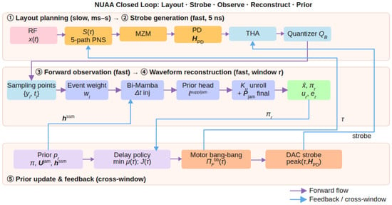
NUAA executes the following five steps at every control step (Figure 2):

Figure 2. NUAA acquisition and reconstruction path. Layout planning, forward observation, online inference, and prior update form a feedback cycle.

• Layout planning: maintain the accumulated coset ${\mathcal{C}}_r$ and belief ${\pi }_r$. When the belief is reliable, minimize the restricted mutual coherence $\mu ({\mathcal{C}}_r\cup \left\{c_{r+1}\right\};{\mathcal{S}}_r)$ [30] over the top-m support ${\mathcal{S}}_r$, and obtain the achievable delay ${\tau }_{r+1}$ via the bang–bang projection ${\Pi }_{\mathcal{F}}^{\mathrm{bb}}$; when the belief is unreliable, fall back to random scanning to maintain broadband measurement diversity.
• Strobe generation: obtain the photonic sampling instants $t_l^{\mathrm{opt}}$ from $\tau$, predict the PD response peak instant $t_i^{\mathrm{smp}}$ with $H_{\mathrm{PD}}$, and drive the DAC strobe.
• Forward observation: $y_r={\mathcal{Q}}_B(S_{\mathrm{smp}}{H}_{\mathrm{THA}}{H}_{\mathrm{PD}}\mathrm{scatter}\left(M_{\mathrm{MZM}}^{\prime }{S}_{\mathrm{opt}}{x}_r\right)+n_r)$; the raw sampling-point stream is fed directly into the learning-based interference identification module, without classical covariance-whitening pre-projection.
• Waveform reconstruction: encode the sampling-point tokens with Bi-Mamba [17] and perform $K_u$ steps of physically consistent unfolding decoding [22,24].
• Prior update and feedback: update ${\pi }_r$ using the measurement–reconstruction correlation energy, and pass $p_{r+1}=\{{\pi }_{r+1},U^{\mathrm{jam}},h^{\mathrm{ssm}},{\widehat{\theta }}_{r+1},\dots \}$ to the next window.

3.2. Feasible Sampling Layouts and Reliability Gating

Over short horizons ($\mathrm{\mu }$s–ms), the EDL layout is nearly frozen, so the NUAA front end reduces to periodic non-uniform sampling (PNS) [9,10]: $L=5$ non-uniform instants $t_l={\sum }_{i=1}^l{\tau }_i$ repeat every master period $T_0=5$ ns. Under the cascaded EDL topology, the coset $c_l=t_l/\eta$ is monotonically non-decreasing and the reachable set is a prefix-sum region rather than five independent sub-bands. The only hard constraint is mutually distinct 1 ps slots (so that $H_{\mathrm{PD}}$ has full rank); overly dense spacing raises $\kappa \left(H_{\mathrm{PD}}\right)$ and is penalized by the soft term $\log \kappa \left(H_{\mathrm{PD}}\right)$ in the layout score $J\left(\tau \right)$, in place of a hard minimum spacing bound.

The layout interface maps abstract cosets to EDL codewords and back. The forward path is: quantize ${\tau }_l\in [0,1000)\mathrm{ps}$ by $\lfloor {\tau }_l/\eta \rfloor$, form the prefix-sum coset, build the grid mask and optical sampling instants $t_l^{\mathrm{opt}}$, and generate the ideal multi-coset row ${[\Phi ]}_{l,k}=\exp (\mathrm{j}2\pi c_{l}k/N_0)$. The inverse path is as follows: the planner’s target coset is mapped to a feasible delay by ${\Pi }_{\mathcal{F}}$, which recovers per-stage increments from adjacent coset differences and enforces reachability ${\dot{\tau }}_l\in \{0,\pm v\}$ with $v=1000\mathrm{ps}/\mathrm{s}$, so that each step lies in $\{0,\pm v\Delta t\}$. Infeasible targets are rewritten, and ${\Pi }_{\mathcal{F}}\left(\mathrm{cosets}\left(\tau \right)\right)=\tau$ holds only at fixed points.

The layout score

$$J\left(\tau \right)=\log \kappa \left(H_{\mathrm{PD}}\right)-{\lambda }_{\mathrm{cnv}}{\sigma }_{\mathrm{cnv}}+{\lambda }_{\mathrm{coh}}{\rho }_{\mathrm{mut}}$$

(11)

is maximized subject to EDL reachability and the ${\Pi }_{\mathcal{F}}$ constraint. When the belief is reliable, the restricted mutual coherence $\mu$ [30] over the top-m support is minimized to drive layout updates; the term $\log \kappa \left(H_{\mathrm{PD}}\right)$ and the conversion window cost term in $J\left(\tau \right)$ explicitly constrain the PD/THA condition number and strobe feasibility, keeping layout planning consistent with the pulse superposition and quantization forward model. NUAA plans the $\tau \left(t\right)$ trajectory under a fixed $f_{\mathrm{avg}}$, and simultaneously reports the first-success time, the delay-trajectory magnitude $\Delta \tau$, and the strobe feasibility rate.

Reliability gating determines that, within the warm-up period of w windows, or when belief concentration is insufficient, the system falls back to random scanning to maintain broadband measurement diversity. Without gating, early incorrect beliefs would make the layout perform worse than random. The gated layout update is executed after Algorithm 1, in Algorithm  2, Steps 5–7.

3.3. Forward Operator Application and Strobe Prediction

Given the physical forward chain $A\left(\tau \right)$ established in Section 2.3, the algorithmic realization treats A as a single calibratable map that concatenates gating, PD/THA pulse superposition, peak readout, and the MZM small-signal slope. Both $S_{\mathrm{opt}}$ and $S_{\mathrm{smp}}$ remain integer-index gathers on the 1 ps grid.

Strobe timing is predicted from the calibrated operator $H_{\mathrm{PD}}$ of Section 2.3. For a given layout $\tau$, the digital back end estimates the photodetector peak instant $t_i^{\mathrm{smp}}$ of each sampling point; a DAC then synthesizes a programmable strobe that drives the THA to sample-and-hold of that peak, after which ${\mathcal{Q}}_B$ (Section 2.2) converts only the held quasi-static level under the acquisition and conversion-window constraints $t_{\mathrm{acq}}=50\mathrm{ps}$ and $t_{\mathrm{cnv}}\ge 200\mathrm{ps}$. The same low-rate quantizer architecture therefore reads programmable non-uniform instants, which lowers the aperture-jitter contribution to ENOB in the forward model.

3.4. Learning-Based Interference Identification and Suppression

Under sub-Nyquist observation [29], noise and strong interference on the $N_{\mathrm{ref}}-M$ unobserved degrees of freedom alias through $A\left(\tau \right)$ into the M-dimensional measurement. At low SIR (e.g., $-40\mathrm{dB}$), folded interference dominates matched-filter peaks and misleads greedy support detection [31]. NUAA identifies useful support, interference atoms, and sample reliability on the raw sampling point stream, then recovers weak components by learning-based subspace nulling and physically consistent unfolding.

Let $\mathcal{C}$ be the in-window candidate set, $A\in {\mathbb{C}}^{M\times \left|\mathcal{C}\right|}$ the dictionary, and $y\in {\mathbb{C}}^M$ the raw measurement. After tokenization (Section 3.5.1) and Bi-Mamba encoding to $q_r$, a shared prior head maps $[m,q_r]$ with $m=A^{H}y$ to

$$\begin{array}{cc}\hfill {\mathsf{\ell }}_j^{\mathrm{supp}},{\mathsf{\ell }}_j^{\mathrm{jam}}& ={\mathrm{PriorHead}}_j\left(\right[\Re m_j,\Im m_j,\log (1 + |m_j\left|\right),q_r\left]\right),\hfill \\ \hfill {\tilde{\pi }}_j^{\mathrm{use}}& =\sigma \left({\mathsf{\ell }}_j^{\mathrm{supp}}\right)\left(1-\sigma \left({\mathsf{\ell }}_j^{\mathrm{jam}}\right)\right).\hfill \end{array}$$

(12)

The logits are supervised by binary cross-entropy (BCE) on useful/interference labels; online, ${\mathsf{\ell }}^{\mathrm{jam}}$ marks strong interference columns. A sample head and anomaly score $a_i$ yield the robust weight

$$w_i=\sigma \left({\mathsf{\ell }}_i^{\mathrm{ev}}\right)\exp (-{\eta }_a{a}_i),A_w=\mathrm{diag}\left(\sqrt{w_i}\right)A,y_w=\mathrm{diag}\left(\sqrt{w_i}\right)y^{\mathrm{base}},$$

(13)

which soft-gates unreliable sampling points in place of $R^{-1/2}$ whitening. A burst head subtracts transient components via $y^{\mathrm{base}}=y-\sigma \left({\mathsf{\ell }}_i^{\mathrm{burst}}\right){\widehat{b}}_i$.

When $\sigma ({\mathsf{\ell }}_{\widehat{j}}^{\mathrm{jam}})>{\tau }_{\mathrm{jam}}$ for $\widehat{j}=\arg {\max }_j\sigma ({\mathsf{\ell }}_j^{\mathrm{jam}})$, a rank-1 projector

$$P_{\mathrm{jam}}=I-{\displaystyle \frac{a_{\widehat{j}}{a}_{\widehat{j}}^H}{\parallel a_{\widehat{j}}{\parallel }_2^2}}$$

(14)

is applied as $y^{\perp }=P_{\mathrm{jam}}{y}_w$ and $A^{\perp }=P_{\mathrm{jam}}{A}_w$. Subsequent data-consistency projection and prior-weighted SOMP–LS refinement on $(A^{\perp },y^{\perp })$ are softly biased by ${\tilde{\pi }}^{\mathrm{use}}$. The algebraic form matches classical $U^{\mathrm{jam}}$, but the interference column is learned rather than greedily selected, reducing erroneous nulling of weak targets.

3.5. Reconstruction Algorithm

NUAA executes Algorithm 1 on a per-window r basis: conditioned on the cross-window prior $p_{r-1}$, ${\widehat{x}}_r$ is recovered from the raw measurement through learning-based preprocessing. The classical reconstruction branch is SOMP [31]/FISTA [32] with a learned prior bias; the FISTA path uses a chirplet/Gabor dictionary [33]; the learning-based reconstruction branch is the proposed NUAA-MU [17,22,24]. After Algorithm 1 completes, Algorithm 2 updates $p_r$ and plans the layout for the next window.

Algorithm 1 NUAA Within-Window Reconstruction (window r)
Input: sampling-point stream ${\left\{(y_i,t_i,l_i)\right\}}_{i=1}^M$, layout ${\tau }_r$, cross-window prior $p_{r-1}=\{{\pi }_r,{\tilde{\pi }}_{r-1}^{\mathrm{use}},\dots \}$. Output: ${\widehat{x}}_r$; if the NUAA-MU path is taken, also output $h_r^{\mathrm{ssm}}$.
1.  $\left\{z_i\right\},{\widetilde{\Delta t}}_i\leftarrow \mathrm{Tokenize}\left(\left\{(y_i,t_i,l_i)\right\}\right)$	(see Section 3.5.1)
2.  $q_r,{\mathsf{\ell }}^{\mathrm{supp}},{\mathsf{\ell }}^{\mathrm{jam}},{\mathsf{\ell }}^{\mathrm{ev}}\leftarrow \mathrm{PriorHead}\left(\mathrm{BiMamba}(\left\{z_i\right\},{\widetilde{\Delta t}}_i)\right)$	(Section 3.4)
3.  $w_i\leftarrow \sigma \left({\mathsf{\ell }}_i^{\mathrm{ev}}\right)\exp (-{\eta }_a{a}_i)$; $y^{\mathrm{base}}\leftarrow y-\sigma \left({\mathsf{\ell }}_i^{\mathrm{burst}}\right){\widehat{b}}_i$; $A_w,y_w\leftarrow \mathrm{diag}\left(\sqrt{w_i}\right)A,\mathrm{diag}\left(\sqrt{w_i}\right)y^{\mathrm{base}}$ 4.  $H_{\mathrm{ev}}\leftarrow S_{\mathrm{smp}}{H}_{\mathrm{THA}}{H}_{\mathrm{PD}}$; $A\left({\tau }_r\right)\leftarrow \mathrm{ColNorm}\left(H_{\mathrm{ev}}{A}_{\mathrm{raw}}\left({\tau }_r\right)\right)$ 5.  $\mathcal{S}\leftarrow \varnothing$, $e\leftarrow y_w$ 6.  for $k=1$ to K do 7.     $j^{★}\leftarrow \arg {\max }_j\left|{\left(A_w^{H}e\right)}_j\right|·(1+\beta {\tilde{\pi }}^{\mathrm{use}}\left(j\right))$ 8.     $\mathcal{S}\leftarrow \mathcal{S}\cup \left\{j^{★}\right\}$; $e\leftarrow y_w-A_{w,\mathcal{S}}{\widehat{x}}_{\mathcal{S}}$
9.  end for	(prior-weighted SOMP)
10.   if reconstruction mode = least squares (LS) then ${\widehat{x}}_r\leftarrow A_{w,\mathcal{S}}^{†}{y}_w$ 11.   else if reconstruction mode = FISTA then ${\widehat{x}}_r\leftarrow \mathrm{FISTA}(y_w;\mathrm{chirplet}/\mathrm{Gabor})$
12.   else ${\widehat{x}}_r,h_r^{\mathrm{ssm}}\leftarrow \mathrm{NUAA}\text{-}\mathrm{MU}(y_w,A_w,p_{r-1})$	(final-step learned $P_{\mathrm{jam}}$ refinement)
13.   end if 14.   return ${\widehat{x}}_r$ (and $h_r^{\mathrm{ssm}}$ if applicable)

3.5.1. Sampling Point Tokenization

After learning-based weighting as in Section 3.4, the M sampling points ${\left\{(y_i,t_i,l_i)\right\}}_{i=1}^M$ within the window are sorted by time, and a token vector $z_i\in {\mathbb{R}}^{d_{\mathrm{in}}}$ is constructed point by point, with the normalized interval ${\widetilde{\Delta t}}_i=\log (1+|\Delta t_i|/T_{\mathrm{ref}})$ kept separately for Bi-Mamba to inject the physical step size.

Let $c_i=t_i/\eta$ be the coset grid index, $s_y$ the 75% quantile of the in-window measurement magnitude, $\mathrm{med}$ and $\mathrm{MAD}$ the median and median absolute deviation of $|y_i|$, respectively, and P the evolution period. With $d_{\mathrm{in}}=10$,

$$\begin{array}{cc}\hfill z_i =& [{\displaystyle \frac{\Re y_i}{s_y}},{\displaystyle \frac{\Im y_i}{s_y}},\log (1+|y_i\left|\right),\mathrm{clip}\left({\displaystyle \frac{|y_i|-\mathrm{med}}{\mathrm{MAD}}}, 0, 20\right),\hfill \\ \hfill & {\displaystyle \frac{c_i}{N_0}},\sin {\displaystyle \frac{2\pi c_i}{N_0}},\cos {\displaystyle \frac{2\pi c_i}{N_0}},{\displaystyle \frac{i}{M}},\sin {\displaystyle \frac{2\pi r}{P}},\cos {\displaystyle \frac{2\pi r}{P}}{]}^{\top },\hfill \end{array}$$

(15)

corresponding, respectively, to the real/imaginary parts of the complex measurement, the log-magnitude, the robust anomaly score, the normalized coset position, the phase-harmonic encoding, the in-window rank, and the cross-window evolution phase. On the candidate-frequency side, a $d_{\mathrm{cand}}=4$-dimensional feature related to the matched-filter response $A^H{y}_w$ is additionally appended, and is concatenated with $q_r$ before being fed into the prior head at the decoding stage. Finally, after linear embedding via $W_{\mathrm{emb}}\in {\mathbb{R}}^{d_{\mathrm{model}}\times d_{\mathrm{in}}}$, a token sequence $\left\{h_i^{\left(0\right)}\right\}$ of length M is obtained and fed into the encoder.

3.5.2. NUAA-MU (Mamba Unfolding Reconstructor)

NUAA-MU implements the learning-based branch of Algorithm 1, Step 12: a Bi-Mamba sampling-point encoder [17], a multi-task prior head (Section 3.4), and a $K_u$-step physically consistent unfolding decoder [22,24]. The encoder stacks $L=2$ ExtBi-Mamba layers ($d_{\mathrm{state}}=24$), each with bidirectional selective state-space modules whose discretization step is the product of a content-dependent term and ${\widetilde{\Delta t}}_i$; after layer normalization, fusion, and residual addition, mean-pooling and a tanh projection yield the window representation $q_r\in {\mathbb{R}}^{d_{\mathrm{model}}}$. The final forward SSM state $h_M^{\mathrm{ssm}}$ is written into $p_{r+1}$ to initialize the next window (bidirectional in training; cross-window SSM memory online).

The decoder performs $K_u=4$ learnable unfolding steps of the form

$${\widehat{x}}^{(k+1)}={\mathcal{D}}_{{\theta }_k}\left({\widehat{x}}^{\left(k\right)}-{\alpha }_k{A}_w^H(A_w{\widehat{x}}^{\left(k\right)}-y_w),q_r\right),$$

(16)

where each ${\mathcal{D}}_{{\theta }_k}$ comprises a two-layer MLP denoise and an SNR-gated complex soft threshold. At the final step, $P_{\mathrm{jam}}$ nulling (Section 3.4) is followed by the hard data-consistency projection $\widehat{x}\leftarrow \widehat{x}-\rho A^{\perp H}(A^{\perp }\widehat{x}-y^{\perp })$ and $K_{\mathrm{sparse}}=3$ steps of prior-weighted SOMP–least-squares refinement. Embedding A at every step prevents a pure sequence model from falling behind classical SOMP [31] under high compression and strong interference. Experiments use the hyperparameters in Table 1 (chirplet dictionary [33] $24\times 8$).

Table 1. NUAA-MU hyperparameter configuration.

Hyperparameter	Value
$d_{\mathrm{model}}$	96
L	2
$d_{\mathrm{state}}$	24
$K_u$	4
$d_{\mathrm{in}}$	10
$n_{\mathcal{C}}$	48
$d_{\mathrm{cand}}$	4
$K_{\mathrm{sparse}}$	3
Parameter count	≈$1.1\times {10}^5$

3.6. Cross-Window Online Accumulation

NUAA accumulates cross-window information in the slow timescale state $p_r$. After Algorithm 1 recovers ${\widehat{x}}_r$, Algorithm 2 writes the belief, learned useful/interference priors, evolution prediction, and encoder memory into $p_{r+1}$, and plans the next layout and strobe. Relative to concatenating historical measurements with differing operators $A\left({\tau }_k\right)$ into one joint equation, this keeps per-window inversion at size $M\times n_{\mathcal{C}}$, adapts to the varying layouts of the EDLs, and supports low-latency streaming without waiting for the full history.

The cross-window state is

$${\theta }^{\mathrm{class}}\oplus p_r={\theta }^{\mathrm{class}}\oplus \{{\pi }_r,{\tilde{\pi }}_r^{\mathrm{use}},{\widehat{\pi }}_r^{\mathrm{jam}},c_r^{\mathrm{cal}},h_r^{\mathrm{ssm}},{\widehat{\mathcal{C}}}_r,\dots \},$$

(17)

where ${\theta }^{\mathrm{class}}$ is the offline scene-class parameter; ${\pi }_r$ is the frequency-domain support belief; ${\tilde{\pi }}_r^{\mathrm{use}},{\widehat{\pi }}_r^{\mathrm{jam}}$ are the learned useful/interference priors; $c_r^{\mathrm{cal}}$ is link calibration; $h_r^{\mathrm{ssm}}$ is the NUAA-MU forward SSM state; and ${\widehat{\mathcal{C}}}_r$ is the predicted tight support set.

The belief ${\pi }_r$ decays toward an in-band uniform prior with forgetting factor $\gamma <1$ and is updated by reconstruction evidence (Algorithm 2, Step 1). An independent GRU evolution head $g_{\varphi }$ is pretrained offline by scene class (radar, frequency hopping, THz communication) and online predicts ${\widehat{\theta }}_{r+1}=g_{\varphi }\left(q_{ \le r}\right)$ with candidate half-width $w_{\mathrm{cand}}\approx 3\%$ of the spectral span, biasing the next SOMP while retaining full-band search (Algorithm 2, Step 3). The drift-to-candidate ratio $\rho =\overline{|\Delta c|}/\left(2w_{\mathrm{cand}}\right)$ gauges predictability: pretraining helps most when $\rho \approx 1$. On the NUAA-MU path, $h_r^{\mathrm{ssm}}$ initializes the next encoder (Algorithm 2, Step 4).

Algorithm 2 NUAA Cross-Window State Update (after window r).
Input: ${\widehat{x}}_r$, $y_w$, $A\left({\tau }_r\right)$, $p_{r-1}$, ${\tau }_r$, window index r; optionally $h_r^{\mathrm{ssm}}$. Output: $p_r$, ${\tau }_{r+1}$, strobe timing table $\left\{{\widehat{t}}_i\right\}$. 1.  ${\pi }_{r+1}\left(\omega \right)\leftarrow \gamma {\pi }_r\left(\omega \right)+(1-\gamma ){\pi }_{\mathrm{uniform}}\left(\omega \right)+\mathrm{softmax}\left(\mathrm{evidence}({\widehat{x}}_r,y_w)\right)$
2.  ${\tilde{\pi }}_{r+1}^{\mathrm{use}},{\widehat{\pi }}_{r+1}^{\mathrm{jam}}\leftarrow \mathrm{EMA}(\sigma ({\mathsf{\ell }}_r^{\mathrm{supp}}),\sigma ({\mathsf{\ell }}_r^{\mathrm{jam}}))$	(EMA of learned useful/interference priors)
3.  ${\widehat{\theta }}_{r+1},{\widehat{\mathcal{C}}}_{r+1}\leftarrow g_{\varphi }\left(q_{ \le r}\right)$	(GRU evolution prediction)
4.  $h_{r+1}^{\mathrm{ssm}}\leftarrow h_r^{\mathrm{ssm}}$ (if the NUAA-MU path; otherwise empty) 5.  if $r<w$ or $\mathrm{Reliable}\left({\pi }_{r+1}\right)=\mathrm{false}$ then ${\tau }_{r+1}\leftarrow \mathrm{RandomScan}\left(\right)$
6.  else ${\tau }_{r+1}\leftarrow \arg {\max }_{\tau \in \mathcal{F}}J\left(\tau \right)$	(reliability-gated layout)
7.  end if 8.  $\left\{{\widehat{t}}_i\right\}\leftarrow \mathrm{PeakTime}({\tau }_{r+1},H_{\mathrm{PD}})$; generate the DAC strobe timing 9.  $p_r\leftarrow \{{\pi }_{r+1},{\tilde{\pi }}_{r+1}^{\mathrm{use}},{\widehat{\pi }}_{r+1}^{\mathrm{jam}},c_r^{\mathrm{cal}},h_{r+1}^{\mathrm{ssm}},{\widehat{\mathcal{C}}}_{r+1},\dots \}$ 10.   return $p_r$, ${\tau }_{r+1}$, $\left\{{\widehat{t}}_i\right\}$

Offline pretraining and online use. Stage A (offline): for each scene class S, evolution sequences $\{x_r,{\theta }_r\}$ drive layout, observation, NUAA-MU reconstruction, and evolution prediction of ${\theta }_{r+1},{\mathcal{C}}_{r+1}$, optimized by $\mathcal{L}={\mathcal{L}}_{\mathrm{rec}}+{\lambda }_{\mathrm{dc}}{\mathcal{L}}_{\mathrm{dc}}+{\lambda }_{\mathrm{sp}}{\mathcal{L}}_{\mathrm{sp}}+{\lambda }_{\mathrm{evo}}{\mathcal{L}}_{\mathrm{evo}}$ to obtain ${\theta }_S^{\mathrm{class}}$. Stage B (online): load ${\theta }_{S^{★}}^{\mathrm{class}}$; each window predicts ${\widehat{\theta }}_r,{\widehat{\mathcal{C}}}_r$ from $g_{\varphi }\left(q_{ < r}\right)$, plans $\tau$, reconstructs, and EMA-updates $p_r$, falling back to ${\tau }_{\mathrm{safe}}$ when the data-consistency residual $\parallel A\widehat{x}{-y\parallel }_2$ rises. Curriculum learning anneals compression and raises interference strength.

Online state machine. Streaming starts from a low-coherence random layout ${\tau }_0$ at $f_{\mathrm{avg}}=1\mathrm{GHz}$. Each window yields ${\widehat{x}}_r$, ${\pi }_r$, and related summaries, then Algorithm 2 updates $p_r$. Reliable belief enables restricted-coherence layout over $\mathcal{F}$; otherwise random scanning is used. Execution switches between static holding ($\Delta \tau =0$) and EDL scanning via ${\Pi }_{\mathcal{F}}^{\mathrm{bb}}$, with DAC strobes from $H_{\mathrm{PD}}$ peak prediction. A rise in $\parallel A\widehat{x}{-y\parallel }_2$ or a drop in belief reliability triggers fallback to ${\tau }_{\mathrm{safe}}$ with exploration.

3.7. Complexity and Online Runtime

The NUAA digital backend implements the observation model in the form of a forward operator: $A\left(\tau \right)$ and its adjoint $A^H$ are applied successively via gated gathering, superposition, and finite-impulse-response convolution, giving a per-iteration complexity of $O(M·n_{\mathcal{C}})$. The computational overhead is analyzed below in terms of the number of samples per reconstruction window M, the candidate dictionary size $n_{\mathcal{C}}$, the sparsity order K, the number of unfolding iteration steps $K_u$, and the hidden layer width $d_{\mathrm{model}}$; the main experiments uniformly adopt $n_{\mathcal{C}}=48$, with the compact NUAA-MU parameter count being $1.1\times {10}^5$ (see Table 1) and the large-capacity streaming model about $4.9\times {10}^5$.

The per-window asymptotic time complexity of each module is summarized in Table 2. Here $L=5$ is the number of samples per master period; m is the belief top-m support size; $n_{\mathrm{cand}}$ is the number of layout candidates scored per search step; $J_{\mathrm{omp}}$ is the number of greedy pursuit iterations inside SOMP/FISTA-style support selection (distinct from the layout score $J\left(\tau \right)$ in Section 3.2); $n_{\mathrm{pass}}$ is the number of belief-gated layout refinement passes per slow-loop tick; $\left|\mathcal{A}\right|$ is the cardinality of the discrete feasible delay/coset action set explored by the search; W is the evolution-GRU lookback length (number of past window embeddings); h is the GRU hidden width; $L_{\mathrm{layer}}$ is the number of Bi-Mamba encoder layers; and $L_{\mathrm{pd}}$ is the FIR support length of the PD/THA kernel on the 1 ps grid.

Table 2. Per-window asymptotic time complexity of NUAA digital modules.

Module	Time Complexity	Remarks
Interference-subspace nulling + SOMP	$O\left(K·(M{n}_{\mathcal{C}}{J}_{\mathrm{omp}}+s^{2}M)\right)$, $s\le K+1$	Classical fast-loop backbone
NUAA-MU encoding	$O(L_{\mathrm{layer}}·M·d_{\mathrm{model}}(d_{\mathrm{model}}+d_{\mathrm{state}}))$	Near-linear in M
NUAA-MU decoding	$O(K_u·M{n}_{\mathcal{C}}+K_u·n_{\mathcal{C}}·d_{\mathrm{model}})$	Same order as SOMP
Layout scoring and strobe prediction	$O(L·L_{\mathrm{pd}})$, $L_{\mathrm{pd}}\ll N_0$	Negligible
Belief-driven layout search	$O(n_{\mathrm{pass}}·L·n_{\mathrm{cand}}·m^2·|\mathcal{A}\left|\right)$	Largest slow-loop cost
Evolution GRU prediction	$O(W·h^2)$	Once per slow-loop tick

In terms of storage overhead, the cross-window belief ${\pi }_r$ occupies $O\left(N_0\right)$ (about 20 KB when $N_0=5000$); the explicit per-window column storage $A\in {\mathbb{C}}^{M\times n_{\mathcal{C}}}$ with $M=200$, the current observation-window samples, and the SSM state together typically require ≲$0.5$ MB; adding the NUAA-MU weights (about 0.4–2 MB depending on capacity) and the evolution head, the resident working set is still ≲3 MB.

Measured Wall-Clock Time (AMD Ryzen AI 9 HX 370)

To complement the asymptotic counts, Table 3 reports single-window wall-clock times on the same CPU used for all simulations in Section 4 (AMD Ryzen AI 9 HX 370, PyTorch CPU inference, version 2.13.0, batch size 1, $M=200$, $n_{\mathcal{C}}=48$, $\mathrm{SNR}=-10$ dB/$\mathrm{SIR}=-40$ dB chirplet window). Chirplet-SOMP finishes in about $0.22$ ms per window. The compact NUAA-MU configuration of Table 1 (≈$1.1\times {10}^5$ parameters) requires about 24 ms per window with refine enabled, occupying about one quarter of the 100 ms slow-loop tick (10 Hz) on this CPU; the large-capacity streaming variant (≈$4.9\times {10}^5$ parameters) requires about $0.69$ s per window and therefore exceeds one tick under the same CPU-only measurement.

Table 3. Measured per-window reconstruction wall-clock time on AMD Ryzen AI 9 HX 370 (PyTorch CPU, batch 1, $M=200$, $n_{\mathcal{C}}=48$).

Method	Parameters	Median Wall Time/Window
chirplet-SOMP	—	$0.22$ ms
NUAA-MU (compact; Table 1)	≈$1.1\times {10}^5$	24 ms
NUAA-MU (large streaming)	≈$4.9\times {10}^5$	$0.69$ s

An order-of-magnitude estimate from Table 2 places the compact model near ${10}^7$ floating-point operations per window ($L_{\mathrm{layer}}=2$, $M=200$, $d_{\mathrm{model}}=96$, $d_{\mathrm{state}}=24$, $K_u=4$, $n_{\mathcal{C}}=48$). The measured 24 ms on CPU is then dominated by interpreter and kernel-launch overhead. GPU, NPU, and FPGA wall-clock times are not measured in this paper. The same operation count can be compared with published peak throughput of those platforms (data-center GPU about 20 TFLOPS in FP32; the HX 370 NPU rating about 50 TOPS in INT8; mid-range FPGA INT8 peaks of order 1–${10}^2$ TOPS), but converting arithmetic volume to latency depends on utilization, on-chip memory, and host I/O. The measured reconstruction time is the 24 ms CPU figure for the compact model.

Layout search remains belief-gated at the slow-loop rate: once priors saturate, random cosets already perform comparably to adaptive layouts, so a full-band Gram search need not run every 5 ns master period. Within each tick the simulated photonic acquisition occupies $0.2\mathrm{\mu }\mathrm{s}$; the remaining ≈100 ms budgets EDL actuation (up to $v\Delta t_{\mathrm{EDL}}\approx 100\mathrm{ps}$ per tick at $v={10}^3\mathrm{ps}/\mathrm{s}$) and digital reconstruction.

4. Simulation Experiment Results

This section evaluates the performance of NUAA on a unified simulation platform. All experiments reported in this paper were conducted on an AMD Ryzen AI 9 HX 370 CPU; the same platform provides the per-window wall-clock times in Table 3 (Section 3.7). The physical forward operator $A\left(\tau \right)$ includes pulse superposition, quantization, and branch gain. Waveform reconstruction is reported via the scale-invariant NMSE (dB). A trial is counted as successful if the in-process NMSE reaches ≤$-10$ dB at least once within the streaming window. The first-success time is the streaming time at which that threshold is first met, and table entries report the median over successful trials only. Sparse support detection is reported via the F1 score (harmonic mean of precision and recall).

Streaming simulation parameters. Unless otherwise noted, each observation window lasts $T_w=0.2\mathrm{\mu }\mathrm{s}$ and comprises 40 master periods ($T_0=5\mathrm{ns}$), yielding $M=200$ sampling points that enter the reconstruction path for that window. Consistent with Section 2.4, $T_0$ is only the optical/PNS clock: physical EDL layouts remain frozen within each $T_w$ and are updated solely on the 100 ms slow layout–inversion tick (the remaining tick time is reserved for EDL adjustment). The default streaming acquisition duration for the main comparison in Table 4 is 200 ms (2 ticks).

Table 4. Streaming broadband chirplet experiment (200 ms, 2 ticks, $\mathrm{SNR}=-10$ dB, $\mathrm{SIR}=-40$ dB; $N_{\mathrm{trial}}=50$). Success rates include Wilson 95% CI; median NMSE values include bootstrap 95% CI where reported.

Method	Success (%)	Atom F1	Median First Success (ms)	Median Final-Tick NMSE (dB)	Median Cumulative-Best NMSE (dB)
Fourier-SOMP	$0[0, 7]$	—	—	≈0	≈0
chirplet-SOMP	$0[0, 7]$	0.43	—	≈0	≈0
prior + EDL scanning	$0[0, 7]$	0.40	—	≈0	≈0
complex ISTA-Net	$0[0, 7]$	0.22	—	≈0	≈0
complex ISTA-Net + scene prior	$20[11, 33]$	1.00	100	$-3.3$ $[-4.1,-2.3]$	$-4.9$ $[-6.0,-3.7]$
complex ISTA-Net + scene prior + classical null	$100[93, 100]$	1.00	100	$-16.0$ $[-16.8,-11.8]$	$-17.3$ $[-20.4,-16.6]$
oracle interference nulling + chirplet-SOMP	$40[28, 54]$	0.64	100	$-5.4$ $[-8.0,-4.4]$	$-7.1$ $[-13.1,-6.1]$
NUAA-MU (no scene prior)	$64[50, 76]$	0.85	200	$-14.7$ $[-18.1,-10.0]$	$-15.0$ $[-18.8,-10.5]$
NUAA-MU + scene prior	$100[93, 100]$	1.00	100	$-27.1$ $[-28.7,-25.6]$	$-28.0$ $[-29.4,-26.8]$

4.1. Broadband Chirp Waveform Reconstruction Under Strong Interference

Signal and interference parameters. Following pulsed-radar convention (pulse width $T_{\mathrm{pw}}$ and PRI satisfying $\mathrm{PRI}\gg T_{\mathrm{pw}}$): pulse width $T_{\mathrm{pw}}=16$ ns (a phase-continuous LFM segment spanning 4 photonic-sampling master periods $T_0=5$ ns), with $K=2$ broadband LFM components per pulse, carrier frequency $f_0\in [20, 120]$ GHz and intrapulse swept bandwidth $B\in [10, 30]$ GHz (chirp rate $k\propto B/T_{\mathrm{pw}}$), each occupying 50–150 frequency-resolution cells on the 1 THz equivalent grid ($\Delta f_{\mathrm{res}}\approx 200$ MHz); the carrier frequency and chirp rate advance across PRIs at a slow timescale following a quasi-periodic evolution law, with $T_{\mathrm{PRI}}=3.2\mathrm{s}$ (asynchronous with $T_0$). A broadband chirp blocking interference is superimposed on the same chirplet grid—carrier likewise in $[20, 120]$ GHz and intrapulse swept bandwidth likewise in $[10, 30]$ GHz—with $\mathrm{SIR}=-40$ dB and a trajectory overlapping the useful component; AWGN is added, with evaluation $\mathrm{SNR}=-10$ dB. The dictionary is a $24\times 8$ chirplet atom grid ($n_{\mathcal{C}}=48$) over this $(f_0,B)$ range.

Experimental setup (oracle-prior regime). Under low-SNR conditions, the experiment adopts static-scene capture: $\alpha$ and the atom support are frozen within the same PRI segment, allowing sampling points to coherently accumulate across master periods $T_0$. The main experimental configuration adopts a Gaussian scene prior centered on the ground-truth atom of the current window, with the candidate chirplet dictionary constructed so that both the ground-truth atom and the interference atom are among the 48 candidates; when the prior peak is ≥$0.9$, the support is locked by the prior top-K, the interference column is nulled after residual correlation detection, and the waveform is estimated by least squares (LS) on the locked support.

A scene prior with this role can be obtained in application from (i) known radar or communication waveform families (band, modulation, pulse width, and PRI) used to pretrain a class model; (ii) coarse spectral occupancy from a companion monitor, injected as a soft prior on the current window; or (iii) support and coefficient statistics accumulated on related tasks in the cross-window state $p_r$. Support locking is used when the merged prior peak is ≥$0.9$: the useful atoms are fixed to the prior top-K, and only the coefficients are then estimated. When the prior is not reliable, support locking is disabled and the useful-support head together with online sufficient statistics discover the support (the no-prior path of Figure 3 and Table 4).

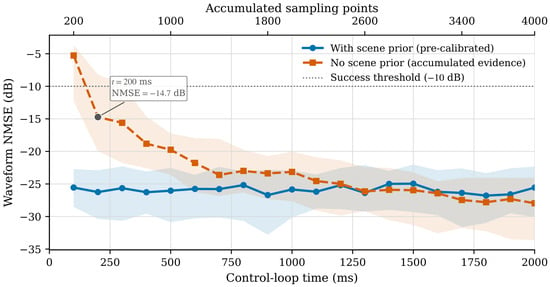
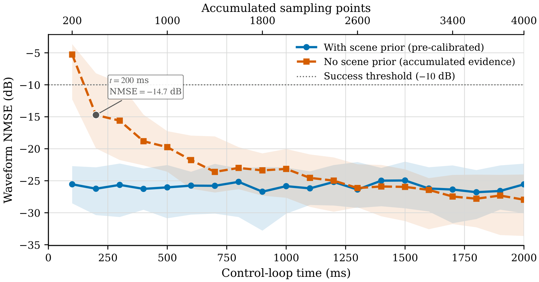
Figure 3. Online evolution of waveform reconstruction NMSE with versus without scene prior. The solid curve is the per-tick median NMSE for the pretrained scene-prior path (20 historical windows, online gain 0.1, coefficient EMA 0.3); the dashed curve with square markers is the autonomous no-prior path. Shaded bands are the interquartile range (IQR, 25th–75th percentile) across $N_{\mathrm{trial}}=50$ trials.

In the controlled study of Figure 3, a NUAA-MU model is pretrained with a scene prior. During online use it retains recurrent adaptation and injects the current-window estimate with gain 0.1 after a mild coefficient EMA of 0.3. The no-prior path starts with no scene prior and accumulates both support and coefficient sufficient statistics ($A^{H}A$, $A^{H}y$) online. This makes the informed curve a low, lightly fluctuating saturated reference. With the scene prior initialized before online use—while the coefficient posterior accumulates online—support F1 is 1.00 from the first tick and the online median NMSE fluctuates lightly around $-25.9$ dB (tick-to-tick standard deviation $0.54$ dB), remaining near $-25.6$ dB at 2 s without exhibiting a sustained downward trend. Without the scene prior, median support F1 rises from 0.50 at 100 ms to 1.00 at 200 ms; as both support confidence and coefficient evidence accumulate, median NMSE decreases from $-5.3$ dB at 100 ms to $-14.7$ dB at 200 ms, $-21.8$ dB at 600 ms and $-28.0$ dB at 2 s, crossing the $-10$ dB success threshold at 200 ms.

The comparison methods include Fourier SOMP, chirplet-SOMP, prior-guided EDL scanning, oracle interference subspace + chirplet-SOMP, and complex ISTA-Net [24] variants—a complex-coefficient realization of the ISTA unrolling network—trained under the same chirplet dictionary and physical measurement model $A\left(\tau \right)$ as NUAA-MU: (i) ISTA-Net without scene prior; (ii) ISTA-Net with scene-prior support locking; and (iii) ISTA-Net with scene-prior locking plus classical residual-correlation jammer nulling. The ISTA-Net reconstructor has ≈$1.9\times {10}^3$ trainable parameters; the compact NUAA-MU model of Table 1 used in this chirplet study has ≈$1.1\times {10}^5$. Unless noted otherwise, Table 4 aggregates $N_{\mathrm{trial}}=50$ independent Monte Carlo trials and reports Wilson 95% confidence intervals for success rates together with bootstrap 95% intervals for median NMSE. A trial succeeds if the in-process NMSE reaches ≤$-10$ dB at least once within the streaming window.

Across the methods in Table 4, the mean fraction of adjacent conversion intervals with a laser-locked THA strobe feasible on the 1 ps grid ($t_{\mathrm{cnv},i}\ge t_{\mathrm{cnv}}^{\min }=200\mathrm{ps}$; Section 2.2) is approximately $0.41$–$0.50$. Success rates count every Monte Carlo trial ($N_{\mathrm{trial}}=50$); infeasible conversion intervals are not dropped from the trial set. Of the nominal $M=200$ samples in a window, about half complete a valid THA conversion; the remaining intervals inflate conversion noise and are down-weighted in the feature mask, while $J\left(\tau \right)$ applies a hinge penalty to the same constraint. The reported NMSE and success rates therefore already include a reduced number of valid conversions relative to a fully feasible layout. The three blind/weak-prior baselines succeed in $0/50$ trials, with median waveform NMSE ≈ 0 dB. The learning-based complex ISTA-Net without a scene prior likewise fails under $\mathrm{SIR}=-40$ dB (success $0\%$, F1 = 0.22). Scene-prior support locking alone raises the ISTA-Net atom F1 to 1.00 but leaves the waveform NMSE near $-3$ dB (success $20\%$, Wilson 95% CI $[11, 33]\%$), because strong interference continues to bias the locked least-squares coefficients. Adding classical residual-correlation jammer nulling before the prior-locked solve restores a $100\%$ success rate ($[93, 100]\%$) and a cumulative-best NMSE of $-17.3$ dB—better than oracle-null chirplet-SOMP ($-7.1$ dB; success $40\%$, $[28, 54]\%$) yet still about 11 dB short of NUAA-MU with scene prior ($-28.0$ dB). Given the ≈$50\times$ parameter gap between ISTA-Net and compact NUAA-MU under the matched dictionary and $A\left(\tau \right)$, this margin mixes capacity with architecture: non-uniform sampling-point sequence encoding and learned interference handling under the physical operator remain the distinctive NUAA-MU ingredients beyond matched-dictionary unrolled sparse reconstruction alone.

Recent photonic reconstruction and sensing methods do not share the operator $A\left(\tau \right)$, so their error metrics are not entered in Table 4. Spectral-encoded single-shot inversion [4] recovers a waveform from a dispersive spectral code. Microwave photonic frequency measurement and time–frequency analysis [5] report occupancy or a spectrogram at about $10\mathrm{ns}$ time resolution. Time-demultiplexing photonic ADCs [7,8] digitize with a full electronic backend near Nyquist. Digital unrolled networks such as ISTA-Net [24] can be compared under the same dictionary and $A\left(\tau \right)$, which is the role of the three ISTA-Net rows in Table 4.

Under scene-prior locking, the NUAA-MU atom F1 is already 1.00 from the first tick, and all $50/50$ trials succeed within 200 ms—matching the 200 ms window of Figure 3. Relative to the oracle interference-nulling baseline, the complete pipeline raises the success rate from $40\%$ to $100\%$ and improves the cumulative-best NMSE by about 21 dB ($-28.0$ vs. $-7.1$ dB), with the gain coming from learned interference identification and locked LS that requires no ramp-up period. With the scene prior removed, the autonomous path in the short 200 ms window of Table 4 reaches $64\%$ success ($[50, 76]\%$) with cumulative-best NMSE $-15.0$ dB—below the result with a scene prior—while Figure 3 shows that a dedicated no-prior model can still drive the median across $-10$ dB by 200 ms and continue improving over the full 2 s horizon.

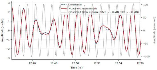
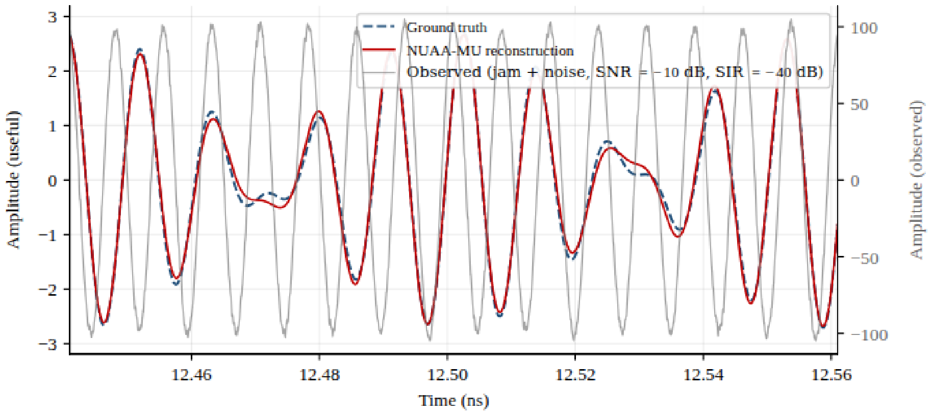
The $T_{\mathrm{pw}}=16$ ns pulse width of the chirp signal requires coherent coverage of multiple $T_0$ segments within each observation window ($T_w=0.2\mathrm{\mu }\mathrm{s}$, 40 master periods, $M=200$). With scene-prior pre-training, support F1 is already 1.00 and the $-10$ dB success criterion is met from the first 100 ms tick; at the 200 ms window of Table 4/Figure 3, the median final-tick NMSE is $-27.1$ dB and the cumulative-best NMSE is $-28.0$ dB. Over the longer 2 s horizon of Figure 3, the with-prior median remains in a low-variance saturated band around $-25.9$ dB (tick-to-tick standard deviation $0.54$ dB). Mechanistically, prior-locked least squares on the observation window recovers the intra-pulse coherent waveform above the strong blocking-interference floor; Figure 4 shows a ∼10-cycle segment whose window NMSE is about $-22.7$ dB.

Figure 4. Comparison of the broadband chirp signal waveform (a segment of ∼10 cycles; left axis: interference-free, noise-free ground truth vs. NUAA-MU reconstruction; right axis: observed waveform with strong interference and AWGN).

4.2. Continuous Tracking of Quasi-Periodically Evolving Complex Intra-Pulse Modulated Radar Waveforms

Signal parameters. Four families of intra-pulse modulation are selected: NLFM, polyphase-coded LFM (polyphase-LFM), Costas intra-pulse frequency-hopping code, and Frank polyphase code; the intra-pulse code length is 64 chips. The initial carrier frequency $f_0\in [20, 60]$ GHz is drawn uniformly, with intra-pulse instantaneous bandwidth $B=20$ GHz. The pulse repetition interval is $T_{\mathrm{PRI}}=10$ ms. This experiment is conducted under a quasi-periodic evolution setting. The carrier frequency drifts within $\pm 6$ GHz under a multi-component sinusoidal law and the codeword index steps periodically. The characteristic periods of this inter-PRI drift are on the order of ${10}^2\mathrm{ms}$ to $1\mathrm{s}$ ($\mathcal{O}\left(10\right)$–$\mathcal{O}\left({10}^2\right)$ PRIs). The SNR is $-10$ dB.

Codebook and streaming interface. A shared radar-class NUAA-MU model is pretrained over the four modulation families using a feature-matched codebook indexed by carrier frequency, instantaneous bandwidth, and discrete codeword ($n_{\mathcal{C}}=48$). During streaming inference, a GRU evolution prior predicts the carrier-center state at the next observation time, while the learned useful prior and the measurement-derived candidate belief are updated by EMA and fused before the next NUAA-MU inversion. Four historical windows initialize this dynamic state before the streaming interval.

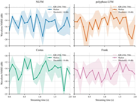
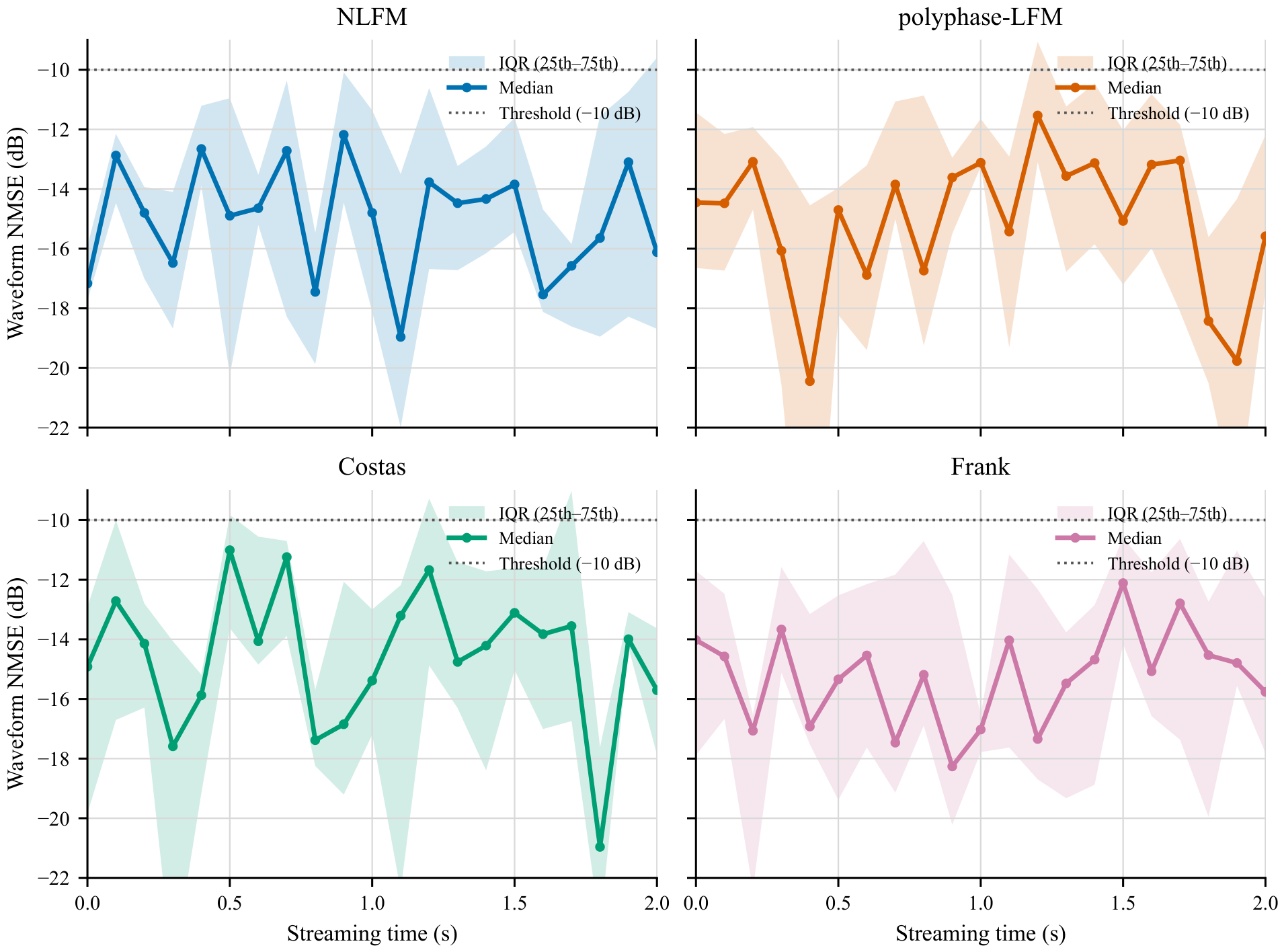
Method and metrics. For each family, $N_{\mathrm{trial}}=50$ trajectories are tracked from 0 to 2 s at 100 ms intervals. Each observation uses one $T_w=0.2\mathrm{\mu }\mathrm{s}$ window with $M=200$ non-uniform samples at $\mathrm{SNR}=-10$ dB. The EDL follows belief-guided updates at $v=1000$ ps/s. A trial succeeds if the NMSE reaches ≤$-10$ dB. Curves in Figure 5 report the per-time NMSE median and IQR across trials.

Figure 5. NUAA-MU waveform reconstruction NMSE for quasi-periodically evolving radar waveforms over 0–2 s. In each panel the solid curve is the per-time median and the shaded band is the IQR across $N_{\mathrm{trial}}=50$ trials; the dotted line marks the $-10$ dB success threshold.

The offline evolution predictor reduces the validation carrier-center MAE from 36.9 slots for persistence prediction to 15.2 slots. Across all four quasi-periodic trajectories, the median NMSE remains below the $-10$ dB threshold throughout 0–2 s. The final median NMSE lies between $-14.3$ and $-15.8$ dB, while the cumulative-best median reaches $-26.9$ to $-30.7$ dB. NLFM, polyphase-LFM, and Costas retain the exact trajectory atom at every observation; Frank has occasional code-trajectory ambiguity (final support-hit rate about $68\%$), but its median carrier-center error remains zero and all waveform trials still satisfy the NMSE criterion. Along the trajectories the per-time median NMSE stays within approximately $-16.7$ to $-13.0$ dB, while the IQR bands typically span about $-21$ to $-10$ dB; these fluctuations therefore reflect the changing trajectory-conditioned measurement geometry and finite-SNR coefficient error rather than loss of quasi-periodic tracking.

4.3. Reconstruction of Terahertz Signals

Signal parameters. As a numerical example on the 1 THz equivalent grid of the NUAA framework, the carrier frequency is set to $f_c\approx 300$ GHz. Distortion is injected onto the periodic spectral support near the carrier frequency (a Gaussian blob approximating the carrier energy distribution), and the SNR is 5 dB. Within each 2 s trial, the carrier support, spectral coefficients, candidate set, and test frame are fixed, while the measurement noise and feasible EDL layout evolve across ticks. The frame bit content does not participate in prior computation.

Method and metrics. Three methods are compared: prior-free SOMP, prior-weighted SOMP (explicit Gaussian carrier neighborhood prior at inversion), and NUAA-MU (pretrained prior). Each method is evaluated over $N_{\mathrm{trial}}=50$ trials and 20 ticks (2 s), with one $T_w=0.2\mathrm{\mu }\mathrm{s}$, $M=200$ observation window every 100 ms. Physical EDL codewords obey the $v=1000$ ps/s constraint of Section 2.4 and therefore remain frozen within each observation window; layout updates occur only across slow-loop ticks. The $M=200$ sensing matrix used inside a window is a digitally synthesized multi-coset measurement stack that matches the diverse $M=200$ training distribution of NUAA-MU (one L-slot row indexed by the master-period index in the simulator). Injected frontend EVM is swept from $0\%$ to $22\%$. Residual constellation EVM is weighted by a squared carrier-hit credit before that format prior, then summarized by the per-point median across trials. The NUAA-MU coefficient solve uses relative Tikhonov regularization $3\times {10}^{-3}$ on the selected support. Unless noted otherwise, the chirplet and radar studies use the compact NUAA-MU hyperparameter set of Table 1 (≈$1.1\times {10}^5$ parameters; ≈24 ms per window in Table 3). The THz reconstruction uses the large-capacity streaming configuration (≈$4.9\times {10}^5$ parameters; ≈$0.69$ s per window on the same CPU path), so its accuracy claims are reported under that higher-capacity setting.

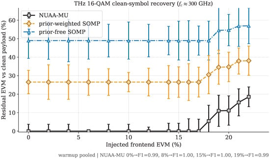
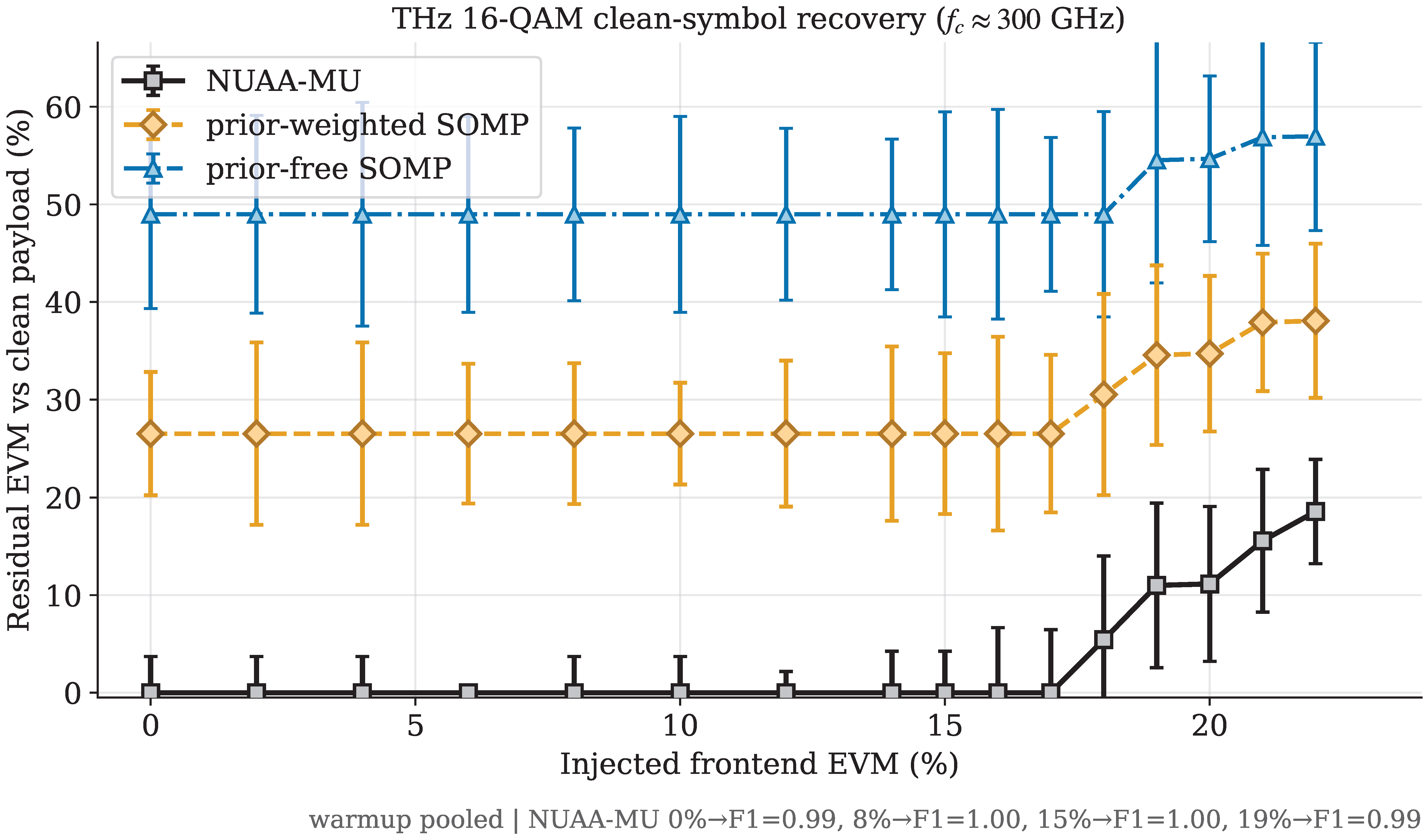
Across the 0–$22\%$ EVM sweep (Figure 6), the three curves separate clearly. Prior-free SOMP remains weakest, with median residual EVM about 49–$57\%$. Prior-weighted SOMP reduces that residual to about 27–$38\%$. NUAA-MU is lowest at all 16 values of injected EVM, with median residual EVM near $0\%$ through $17\%$ injected EVM and about $5.4$–$18.6\%$ from $18\%$ to $22\%$. The margin over prior-weighted SOMP is typically about 20–27 percentage points and remains about $19.5$ pp at $22\%$. The plateaus below $18\%$ are expected under this metric: the seven-bin carrier support and median aggregation yield discrete carrier-hit levels, while correct 16-QAM decisions are projected to the same alphabet points. In particular, the $5/7$ and $6/7$ median support-hit levels of prior-free and prior-weighted SOMP correspond to hit penalties of approximately $49.0\%$ and $26.5\%$, respectively, before residual constellation error becomes appreciable.

Figure 6. Residual constellation EVM versus injected frontend EVM for THz 16-QAM signals from $0\%$ to $22\%$ ($2\%$ steps to $15\%$, then $1\%$ steps; $f_c\approx 300$ GHz; black solid line with square markers: NUAA-MU; amber dashed line with diamond markers: prior-weighted SOMP; blue dash-dotted line with triangular markers: prior-free SOMP). All methods use the same modulation-format prior. Low-EVM plateaus arise from discrete seven-bin support-hit levels and correct 16-QAM alphabet projection.

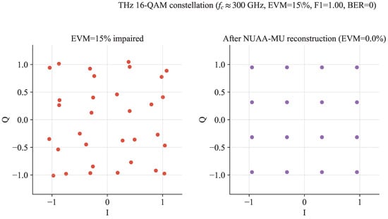
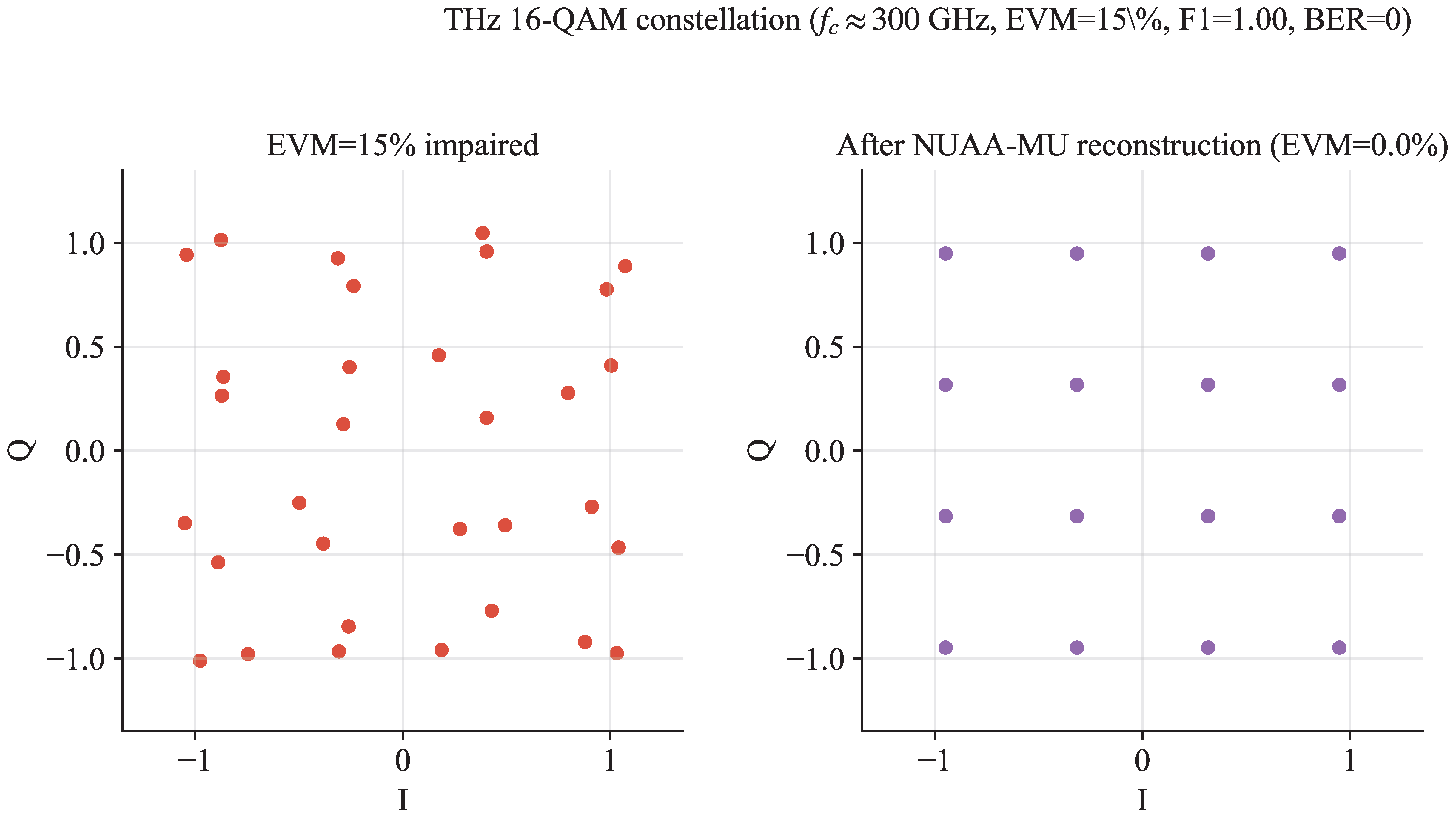
Figure 7 shows a representative $15\%$ injected EVM trial after modulation format projection on the NUAA-MU recovery path. The projected frame has zero symbol errors (and zero bit errors) under hard 16-QAM decisions.

Figure 7. THz 16-QAM constellation at $15\%$ injected EVM (left: EVM impaired; right: after reconstruction by NUAA-MU).

5. Discussion

5.1. Timing Reference, Delay Errors, and Calibration–Prior Equivalence

The mode-locked laser emits a highly stable train of ultrashort optical pulses, which serves as the temporal reference for the equivalent 1 ps grid [7,8]. The THA sampling strobe is synchronized to this pulse train and scheduled relative to the calibrated optical-pulse arrival and PD peak, so residual timing error enters as an effective sampling-phase perturbation of the RF waveform rather than as a free-running electronic clock at the 1 THz equivalent sampling rate. For a carrier near frequency $f_{\mathrm{RF}}$, the first-order phase perturbation scales as $2\pi f_{\mathrm{RF}}{\sigma }_t$. Mode-locked sources routinely provide femtosecond-level residual timing stability; with ${\sigma }_t$ on the order of a few tens of femtoseconds, $2\pi f_{\mathrm{RF}}{\sigma }_t$ remains $\ll 1$ even at $f_{\mathrm{RF}}\approx 300$ GHz, where $1/\left(2\pi f_{\mathrm{RF}}\right)\approx 0.53$ ps. Commanded EDL layouts are likewise required to keep residual positioning error $\left|\epsilon \right|\ll 1/\left(2\pi f_{\mathrm{RF}}\right)$ relative to the calibrated optical timing. Under this laser-locked reference the baseline model therefore folds residual strobe and sub-grid timing error into the ENOB term rather than assigning an independent jitter distribution. The remaining reconstruction sensitivity is set primarily by (i) slow hardware mismatches absorbed into the forward operator and (ii) accumulating EDL command errors relative to the commanded layout $\tau$.

5.1.1. Stable Mismatches as Effective Signal Distortion

Let $\tau$ denote the commanded EDL layout and $A\left(\tau \right)$ the nominal forward operator of Section 2.3. Branch-dependent optical attenuation (unequal pulse amplitudes across the $L=5$ coset slots), non-flat PD/THA frequency response, and related slowly varying gains enter as a stable multiplicative mismatch G (diagonal or block-diagonal on the optical/electrical path). The physical measurement then reads

$$y=A\left(\tau \right)Gx+n=A\left(\tau \right)x_{\mathrm{eff}}+n,x_{\mathrm{eff}}\triangleq Gx.$$

(18)

Thus a class of hardware errors is observationally equivalent to a distorted waveform $x_{\mathrm{eff}}$ under the nominal operator. Because G is stable across windows, it is absorbed by the link-calibration state $c_r^{\mathrm{cal}}$ in the cross-window memory $p_r$ (Section 3.6) or by device-calibrated kernels $H_{\mathrm{PD}}/H_{\mathrm{THA}}$ inside $A\left(\tau \right)$. In either case the inversion remains matched: after calibration the residual behaves as ordinary measurement noise without a structured operator bias. The same reasoning applies when $A\left(\tau \right)$ stays matched to the readout chain under moderate strobe walk/jitter or PD/THA bandwidth variation: residual mismatch is absorbed into calibration or appears as ordinary measurement noise rather than a structured operator bias.

5.1.2. Accumulating Delay Errors Versus Accumulating Priors

EDL tuning is bang–bang-limited at $v=1000$ ps/s. Commanded increments therefore realize

$${\tau }_{r+1}^{\mathrm{phys}}={\tau }_r^{\mathrm{phys}}+\Delta {\tau }_r+{\epsilon }_r,$$

(19)

where $\Delta {\tau }_r$ is the intended slow-loop update and ${\epsilon }_r$ collects per-tick positioning error (quantization to $\eta =1$ ps, mechanical backlash, and residual calibration drift). Relative to an RF carrier near $f_{\mathrm{RF}}$, the design target is $\parallel {\epsilon }_r\parallel \ll 1/\left(2\pi f_{\mathrm{RF}}\right)$ after calibration; residual error above that scale appears as the structured operator perturbation below. First-order expansion of the operator about the commanded layout yields

$$A\left(\tau +\epsilon \right)x=A\left(\tau \right)x+\sum _i{\epsilon }_i{\partial }_{{\tau }_i}A\left(\tau \right)x+O({\parallel \epsilon \parallel }^2),$$

(20)

so an uncompensated delay error again appears as an additive structured residual—equivalently, a layout-dependent signal distortion under the commanded $A\left(\tau \right)$. Concurrently, the online pathway accumulates belief and useful/interference priors $({\pi }_r,{\tilde{\pi }}_r^{\mathrm{use}},{\widehat{\pi }}_r^{\mathrm{jam}})$ from the streaming measurements (Section 3.6; Figure 3). When the belief is reliable, layout updates minimize restricted mutual coherence on the believed support; when it is not, the planner falls back to random scanning. The two accumulations therefore counteract: delay error injects structured mismatch, while prior accumulation concentrates subsequent measurements on the recoverable support and continually re-anchors $c_r^{\mathrm{cal}}$ and $A\left(\tau \right)$ to the observed chain.

5.1.3. Calibration–Prior Equivalence

Initialization self-calibration of branch gains, strobe peak predictors, and kernel parameters can be written as an offline estimate ${\widehat{c}}_0^{\mathrm{cal}}$ inserted into $p_0$. For the streaming analysis, this is equivalent to a pretrained scene/link prior: both supply a low-entropy starting state that reduces early-window innovation. Online, calibration updates and prior updates share the same sufficient-statistic pathway,

$$p_{r+1}=\mathrm{EMA}\left(p_r,\mathrm{evidence}({\widehat{x}}_r,y_r;A\left({\tau }_r\right))\right),$$

(21)

so improving $c_r^{\mathrm{cal}}$ (operator matching) and sharpening ${\pi }_r$ (scene matching) are two faces of one accumulation. In short: stable system errors are equivalent to signal distortion under a mismatched operator and are removed by calibration; accumulating delay errors are equivalent to layout-dependent distortion and are offset by accumulating feature priors; and system calibration is operationally equivalent to prior accumulation in the cross-window state $p_r$. Delay positioning accuracy, branch-to-branch loss consistency, and the realized non-uniform sampling sequence therefore enter the same state: residual delay and gain errors are absorbed as effective signal distortion under $A\left(\tau \right)$, and online evidence updates both the operator match and the scene prior.

5.2. Scope, Photonic Novelty, and Simulation Validation

NUAA is framed as an adaptive microwave photonic A2I conversion framework [10,25,26]: a mode-locked laser, cascaded EDLs, MZM, band-limited PD/THA, and a low-rate quantizer are co-designed with pattern control, prior accumulation, and waveform reconstruction. The photonic novelty is therefore not a new discrete device or module, but the band-limited PD pulse-superposition operator that intentionally operates below the RF support bandwidth and recovers per-pulse amplitudes by invertible overlap under precise optical timing (Section 2.3). Classical A2I/PADC pipelines and photonic spectrum sensors more often emphasize sparse spectrum estimation [4,5,10]; the present design targets active layout adaptation and broadband waveform recovery under strong interference.

The reported results are numerical simulations of $A\left(\tau \right)$. Each comparison uses a Monte Carlo size of $N_{\mathrm{trial}}=50$, with Wilson intervals on success rates and bootstrap intervals on median NMSE, so that the margins between methods include their statistical uncertainty. Results with a scene prior and without a scene prior are tabulated and plotted separately, which isolates the contribution of the prior from that of the acquisition path. A learning-based complex ISTA-Net baseline shares the chirplet dictionary and the physical operator $A\left(\tau \right)$ with NUAA-MU, so the comparison reflects the reconstructor rather than a difference in the forward model. The three timescales of Section 2.4 are respected throughout: physical layouts stay fixed within $T_w$, and the multi-coset stacks that supply training diversity are digital constructions. Per-window wall-clock times are measured on the AMD Ryzen AI 9 HX 370 CPU used for all simulations; GPU, NPU, and FPGA times in Section 3.7 are operation-count comparisons with published peak throughput. Finally, Section 5.1 treats timing jitter, delay errors, and calibration within one framework, showing which hardware imperfections are absorbed by the calibrated operator and which remain as residual noise.

5.3. Photonic–Algorithm Co-Design

Microwave photonics began as a fusion of microwave engineering and photonics. As Yao and Capmany argue, further progress now calls for broader synergy that also draws materials, electronics, software, and system architectures into one co-design, including architectures driven by AI, because no single platform can meet bandwidth, energy, and functional-density demands alone [34]. NUAA instantiates that agenda as joint acquisition and reconstruction: layout and strobe commands shape the measurements, while priors and reconstructors exploit those measurements under a physically consistent operator. A controller driven by learning plans non-uniform optical sampling patterns and accumulates feature priors; the photonic link (mode-locked laser, cascaded EDLs, MZM, band-limited PD/THA) supplies the programmable timing and invertible superposition measurements used by the algorithm.

6. Conclusions

This paper proposes NUAA, a non-uniform adaptive photonic sampling framework for broadband electromagnetic waveform reconstruction. In the simulated front end, a cascaded prefix-sum electrical optical delay line generates a non-uniform sample stream with an average sampling rate of 1 GHz on a 1 ps equivalent grid. Non-uniform readout is modeled by a THA and a pure quantizer driven by algorithm-predicted strobes, and the digital back end performs feature-matched reconstruction using the physically consistent operator $A\left(\tau \right)$, an interference subspace, an online belief, and an offline evolution prior. All reported reconstruction metrics are obtained from numerical simulations of this forward operator. The 1 THz figure is the equivalent Nyquist rate of the 1 ps EDL grid.

The simulation results show that with a scene prior and support locking, on the frequency-domain non-sparse broadband chirplet streaming task ($T_{\mathrm{pw}}=16$ ns, $\mathrm{PRI}=3.2\mathrm{s}$, $\mathrm{SNR}=-10$ dB, $\mathrm{SIR}=-40$ dB; $N_{\mathrm{trial}}=50$), NUAA-MU reaches F1 = 1.00 and a 100% success rate within 200 ms (Wilson 95% CI $[93, 100]\%$; cumulative-best NMSE $-28.0$ dB), about 21 dB better than the oracle baseline under the same setting (40% success rate, $[28, 54]\%$; cumulative-best NMSE $-7.1$ dB); the corresponding configuration without a scene prior reaches only $64\%$ success ($[50, 76]\%$) in the same 200 ms window. On quasi-periodically evolving NLFM, polyphase-LFM, Costas, and Frank waveforms, the pretrained evolution prior with online EMA updates maintains 100% waveform success over 0–2 s, with final median NMSE $-14.3$ to $-15.8$ dB. For a simulated 16-QAM communication example at $f_c\approx 300$ GHz, NUAA-MU yields the lowest residual constellation EVM across the 0–$22\%$ injected EVM sweep (near $0\%$ through $17\%$ injected EVM; about $5.4$–$18.6\%$ from $18\%$ to $22\%$), typically 20–27 percentage points below prior-weighted SOMP.

Taken together, the experiments above show that NUAA’s gain comes from matching three conditions (Table 5):

Table 5. Three matching conditions underlying NUAA performance gains.

Condition	Representative Experiment	Consequence of Mismatch
Physical operator matching	Section 2.3, Section 2.4, Section 3.1, Section 3.2 and Section 3.3: $A\left(\tau \right)$ forward model	Readout band-limiting and pulse superposition are mis-modeled, degrading support recovery
Measurement diversity matching	Section 3.2 and Section 4.1: layout diversity, interference-subspace nulling	Static layout has insufficient rank, and folded strong interference hijacks the support
Prior predictability matching	Section 4.1, Section 4.2 and Section 4.3: broadband-to-terahertz streaming/evolution prior	Capacity and adaptation are ineffective on random or unstructured signals

This paper still has boundaries. The evolution prior depends on scene structure. The two-level prior is applicable to low-entropy, predictable evolution; when the innovation ${ϵ}_r$ increases or the underlying law changes abruptly, the benefit decreases, and layout adaptation is not universally superior to random scanning, especially in some highly dynamic scenarios. Nevertheless, real-world RF waveforms almost always exhibit partial regularity that can be absorbed into feature priors. Even without offline pretraining, NUAA can accumulate belief and useful/interference priors online from the streaming measurements. This online prior pathway is what sustains the advantage of the proposed scheme under practical operating conditions. Moreover, key system parameters—including the number of cascaded optical delay-line stages, the optical pulse repetition frequency, and the resulting average sampling rate—can be flexibly reconfigured to match different application scenarios.

References

- Bai, Y.; Liu, Z.; Duan, M.; Feng, J.; Xiong, X.; Wei, K.; Wu, K.; Jia, X.; Liao, R.; Song, Y.; et al. Microwave photonic links and transversal microwave photonic applications. Electromagn. Sci. 2025, 3, 0090541. [Google Scholar] [CrossRef] [Scilit]
- Podbregar, L.; Batagelj, B.; Blatnik, A.; Lavrič, A. Advances in and applications of microwave photonics in radar systems: A review. Photonics 2025, 12, 529. [Google Scholar] [CrossRef] [Scilit]
- Mahammedi, N.A.; Vasquez-Peralvo, J.A.; Masood, R.; Merlano-Duncan, J.C.; Guzmán Martínez, R.C.; Chatzinotas, S. Photonic digital-to-analog converters (PDACs): Architectures, performances, and technology roadmaps. TechRxiv 2025. [Google Scholar] [CrossRef] [Scilit] [PubMed]
- Kang, M.; Underwood, T.C. Single-shot spectral-encoded waveform reconstruction through probabilistic inversion. arXiv 2026, arXiv:2606.14936. [Google Scholar] [CrossRef] [Scilit]
- Shi, T.; Jiang, C.; Lin, C.; Yang, F.; Liu, Y.; Zhang, F.; Chen, Y. Microwave photonic frequency measurement and time–frequency analysis: Unlocking bandwidths over hundreds of GHz with a 10-nanosecond temporal resolution. IEEE Trans. Microw. Theory Techn. 2025, 73, 4104–4115. [Google Scholar] [CrossRef] [Scilit]
- Haigh, K.; Andrusenko, J. Cognitive Electronic Warfare: An Artificial Intelligence Approach; Artech House: Norwood, MA, USA, 2021. [Google Scholar]
- Qin, R.; Qian, N.; Zhou, D.; Ma, B.; Zou, W. Decoupling and one-time elimination of the timing skew in a time-demultiplexing photonic analog-to-digital converter for high-resolution wideband signal acquisition. Opt. Lett. 2023, 48, 5324–5327. [Google Scholar] [CrossRef] [Scilit] [PubMed]
- Qi, J.; Chen, X.; Fu, M.; Zhang, H.; Yi, W.; Xu, T.; Su, D.; Zhang, H.; Wei, X.; Shi, B.; et al. Effects of optical sampling pulse power, RF power, and electronic back-end bandwidth on the performance of photonic analog-to-digital converter. Micromachines 2023, 14, 2155. [Google Scholar] [CrossRef] [Scilit] [PubMed]
- Venkataramani, R.; Bresler, Y. Perfect reconstruction formulas and bounds on aliasing error in sub-Nyquist nonuniform sampling of multiband signals. IEEE Trans. Inf. Theory 2000, 46, 2173–2183. [Google Scholar] [CrossRef] [Scilit]
- Mishali, M.; Eldar, Y.C. From theory to practice: Sub-Nyquist sampling of sparse wideband analog signals. IEEE J. Sel. Top. Signal Process. 2010, 4, 375–391. [Google Scholar] [CrossRef] [Scilit]
- Wang, J.; Huang, Y.; Wang, B. Sub-Nyquist sampling-based wideband spectrum sensing: A compressed power spectrum estimation approach. Front. Comput. Sci. 2023, 18, 182501. [Google Scholar] [CrossRef] [Scilit]
- Lin, R.; Shen, Y.; Chen, Y. Dual-ascent-inspired Transformer for compressed sensing. Sensors 2025, 25, 2157. [Google Scholar] [CrossRef] [Scilit] [PubMed]
- Machidon, A.L.; Pejović, V. Deep learning for compressive sensing: A ubiquitous systems perspective. Artif. Intell. Rev. 2023, 56, 3619–3658. [Google Scholar] [CrossRef] [Scilit]
- Chen, Y.; Ren, K.; Wang, Y.; Fang, Y.; Sun, W.; Li, D. ContiFormer: Continuous-time Transformer for irregular time series modeling. In Advances in Neural Information Processing Systems; Oh, A., Naumann, T., Globerson, A., Saenko, K., Hardt, M., Levine, S., Eds.; Curran Associates, Inc.: Red Hook, NY, USA, 2023; Volume 36, pp. 47143–47175. [Google Scholar]
- Wei, Y.; Peng, J.; He, T.; Xu, C.; Zhang, J.; Pan, S.; Chen, S. Compatible Transformer for irregularly sampled multivariate time series. In Proceedings of the IEEE International Conference on Acoustics, Speech and Signal Processing (ICASSP), Seoul, Republic of Korea, 14–19 April 2024. [Google Scholar]
- Uray, M.; Geng, D.; Graf, F.; Huber, S.; Kwitt, R. Anomaly detection for sparse and irregular multivariate time series with latent SDEs. arXiv 2026, arXiv:2606.18898. [Google Scholar] [CrossRef] [Scilit]
- Gu, A.; Dao, T. Mamba: Linear-time sequence modeling with selective state spaces. In Proceedings of the International Conference on Machine Learning (ICML), Vienna, Austria, 21–27 July 2024. [Google Scholar]
- Nguyen, T.T.; Jin, M.; Pham, T.; Pan, S.; Nguyen, Q.V.H. Mamba for time series analysis: A contemporary survey. Preprints 2026. [Google Scholar] [CrossRef] [Scilit]
- Solís-García, J.; Vega-Márquez, B.; Nepomuceno, J.A.; Nepomuceno-Chamorro, I.A. TIMBA: Time series imputation with bi-directional Mamba blocks and diffusion models. arXiv 2024, arXiv:2410.05916. [Google Scholar] [CrossRef] [Scilit]
- Liang, A.; Jiang, X.; Sun, Y.; Shi, X.; Li, K. Bi-Mamba+: Bidirectional Mamba for time series forecasting. arXiv 2024, arXiv:2404.15772. [Google Scholar] [CrossRef] [Scilit]
- Hu, J.; Luo, G.; Lan, D.; Wen, Q.; Zhou, Z.; Liang, Y. How to train your Mamba for time series forecasting. In Proceedings of the 32nd ACM SIGKDD Conference on Knowledge Discovery and Data Mining (KDD), Jeju Island, Republic of Korea, 9–13 August 2026. [Google Scholar] [CrossRef] [Scilit]
- Fang, P.; Chen, H.; Tang, F.; Liu, F.; Cai, X.; Shan, S. SO-Mamba: State-ownership Mamba for unrolled MRI reconstruction. arXiv 2026, arXiv:2605.22031. [Google Scholar] [CrossRef] [Scilit]
- Gao, X.; Chen, B.; Yao, X.; Yuan, Y. SSM-Net: Enhancing compressed sensing image reconstruction with Mamba architecture and fast iterative shrinking threshold algorithm optimization. Sensors 2025, 25, 1026. [Google Scholar] [CrossRef] [Scilit] [PubMed]
- Zhang, J.; Ghanem, B. ISTA-Net: Interpretable optimization-inspired deep network for image compressive sensing. In Proceedings of the IEEE/CVF Conference on Computer Vision and Pattern Recognition (CVPR), Salt Lake City, UT, USA, 18–22 June 2018; pp. 1828–1837. [Google Scholar]
- Fu, N.; Zhang, J. Analog-to-Information Conversion Technology Based on Compressed Sensing; Tsinghua University Press: Beijing, China, 2020. (In Chinese) [Google Scholar]
- Laska, J.; Kirolos, S.; Massoud, Y.; Baraniuk, R.; Gilbert, A.; Iwen, M.; Strauss, M. Random sampling for analog-to-information conversion of wideband signals. In Proceedings of the IEEE Dallas Circuits and Systems Workshop, Dallas, TX, USA, 29–30 October 2006; pp. 119–122. [Google Scholar]
- Piprek, J. Semiconductor Optoelectronic Devices: Introduction to Physics and Simulation; Academic Press: San Diego, CA, USA, 2003. [Google Scholar]
- Oppenheim, A.V.; Willsky, A.S.; Nawab, S.H. Signals and Systems, 2nd ed.; Prentice Hall: Upper Saddle River, NJ, USA, 1997. [Google Scholar]
- Donoho, D.L. Compressed sensing. IEEE Trans. Inf. Theory 2006, 52, 1289–1306. [Google Scholar] [CrossRef] [Scilit]
- Donoho, D.L.; Huo, X. Uncertainty principles and ideal atomic decomposition. IEEE Trans. Inf. Theory 2001, 47, 2845–2862. [Google Scholar] [CrossRef] [Scilit]
- Tropp, J.A.; Gilbert, A.C.; Strauss, M.J. Algorithms for simultaneous sparse approximation. Part I: Greedy pursuit. Signal Process. 2006, 86, 572–588. [Google Scholar] [CrossRef] [Scilit]
- Beck, A.; Teboulle, M. A fast iterative shrinkage-thresholding algorithm for linear inverse problems. SIAM J. Imaging Sci. 2009, 2, 183–202. [Google Scholar] [CrossRef] [Scilit]
- Mann, S.; Haykin, S. The chirplet transform: Physical considerations. IEEE Trans. Signal Process. 1995, 43, 2745–2761. [Google Scholar] [CrossRef] [Scilit] [PubMed]
- Yao, J.; Capmany, J. The age of photonic synergy: Why no single platform can drive the future alone. PhotoniX Synerg. 2026, 1, 1. [Google Scholar] [CrossRef] [Scilit]
Disclaimer/Publisher’s Note: The statements, opinions and data contained in all publications are solely those of the individual author(s) and contributor(s) and not of MDPI and/or the editor(s). MDPI and/or the editor(s) disclaim responsibility for any injury to people or property resulting from any ideas, methods, instructions or products referred to in the content. |
© 2026 by the author. Licensee MDPI, Basel, Switzerland. This article is an open access article distributed under the terms and conditions of the Creative Commons Attribution (CC BY) license.