A Large-Field Photoacoustic-OCT Dual-Modal Imaging System Based on Temporal Medium Separation and Hardware-Based Coordinate Locking

Abstract

Optical coherence tomography (OCT) and photoacoustic imaging (PAI) provide complementary structural and absorption contrasts but require different coupling conditions: 1310 nm swept-source OCT is attenuated by water, whereas PAI requires acoustic coupling. We developed a large-field dual-modal imaging system combining temporal medium separation with hardware-based coordinate locking. The OCT head, linear-array ultrasound transducer, and photoacoustic excitation fiber bundle were mounted on a rigid common platform, and a one-time calibration established a two-dimensional affine transformation between the modality coordinate systems. OCT was acquired in air and PAI in deionized water within a common large-field coordinate range. In five paired air–water measurements with an approximately 23 mm water path, the displayed OCT peak level decreased from 98.4 ± 1.5 dB in air to 79.4 ± 1.8 dB in water, corresponding to a mean reduction of 19.0 ± 1.4 dB. Quantitative registration was evaluated using a 5 × 5 dual-modal landmark phantom, with nine landmarks used for affine calibration and 16 excluded landmarks reserved for independent validation. The mean two-dimensional validation error was 0.235 ± 0.128 mm, with an RMSE of 0.266 mm and a maximum error of 0.446 mm. Five additional medium-switching cycles performed without recalibration yielded an overall registration error of 0.369 ± 0.163 mm across 80 validation measurements. PA spatial resolution was further characterized using six thin hair targets, yielding lateral and axial FWHM values of 0.342 ± 0.069 mm and 0.394 ± 0.073 mm, respectively. These results demonstrate reproducible two-dimensional en face OCT–PA coordinate mapping under modality-specific coupling conditions and support the proposed workflow as a phantom-based technical validation for large-field multimodal imaging.

1. Introduction

Optical coherence tomography (OCT) is a well-established optical imaging modality that uses low-coherence interferometry to provide micrometer-scale, depth-resolved structural information from superficial tissues [1,2,3]. Swept-source OCT (SS-OCT), particularly in the 1300 nm spectral region, enables high-speed volumetric imaging with relatively deep penetration in scattering tissue [3]. However, OCT primarily provides structural contrast and has limited penetration depth compared with acoustic imaging techniques [4,5].

Photoacoustic imaging (PAI), in contrast, combines optical excitation with ultrasonic detection and provides absorption-based contrast at greater imaging depths [6,7,8]. Efficient transmission of the generated acoustic waves generally requires an appropriate coupling medium, such as water or ultrasound gel [9,10]. Consequently, OCT and PAI offer complementary structural and optical-absorption information and have motivated the development of multimodal imaging systems that integrate the two techniques [11,12].

A practical challenge in sequential OCT–PA integration is the difference in their preferred coupling conditions. At wavelengths around 1300 nm, propagation through water can introduce substantial optical loss and alter the OCT imaging condition [13,14], whereas PA detection relies on effective acoustic coupling [15,16]. Previous OCT–PA systems have demonstrated the feasibility of combining these complementary modalities using various optical and acoustic configurations [17,18,19,20]. For example, Park et al. integrated ultrasound, photoacoustic, OCT, and fluorescence imaging using a transparent ultrasound transducer [21]. Such approaches demonstrate the potential of multimodal imaging but may require specialized optical/acoustic components or more complex system architectures.

In addition to coupling-medium compatibility, practical biomedical optical imaging increasingly requires consideration of field of view, acquisition efficiency, motion robustness, signal-to-noise ratio, and spatial correspondence between sequentially acquired datasets. Recent work in biological microscopy has also highlighted the importance of maintaining image fidelity under photon-limited and motion-prone acquisition conditions. For example, Shen et al. developed a self-supervised computational framework to improve biological imaging under photon noise and motion artifacts, illustrating the broader need for robust acquisition and reconstruction strategies in high-throughput optical imaging [22]. For multimodal OCT–PA imaging, these practical considerations are further complicated by spatially separated optical and acoustic paths and the need to preserve correspondence over relatively large scanning regions [23,24].

To address these issues, we developed a large-field photoacoustic–OCT dual-modal imaging system based on temporal medium separation and hardware-based coordinate locking. The OCT scanning head, linear-array ultrasound transducer, and PA excitation fiber bundle are mechanically fixed on a rigid common platform. OCT acquisition is performed in air, after which deionized water is introduced for PA acoustic coupling without repositioning the phantom. A one-time calibration establishes a two-dimensional affine transformation between the PA and OCT en face coordinate systems, which is subsequently reused without feature-based post-registration.

The present study focuses on phantom-based technical validation of this workflow. In addition to demonstrating complementary large-field OCT and PA imaging, we quantitatively evaluate the OCT signal change between air and water conditions, full-field two-dimensional registration accuracy using calibration and independent validation landmarks, registration repeatability over repeated medium-switching cycles without recalibration, and the FWHM-based spatial response of the PA subsystem using thin hair targets. The current implementation is therefore intended to establish the feasibility and repeatability of two-dimensional en face OCT–PA coordinate mapping, rather than full three-dimensional co-registration or biological imaging performance.

2. Materials and Methods

2.1. System Overview

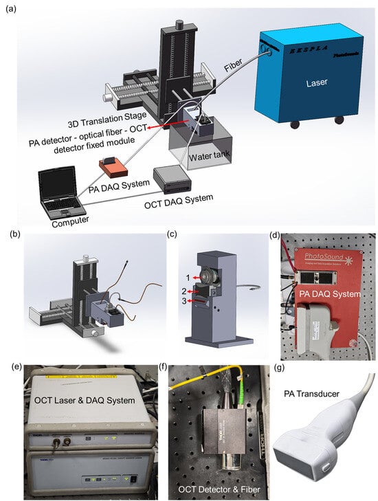
A schematic of the proposed large-field photoacoustic–OCT dual-modal imaging system is shown in Figure 1. The system integrates three core modules—photoacoustic excitation, ultrasound detection, and swept-source OCT—on a rigid common-mode positioning platform, enabling temporal medium separation while maintaining a stable mechanical relationship between the two imaging modalities.

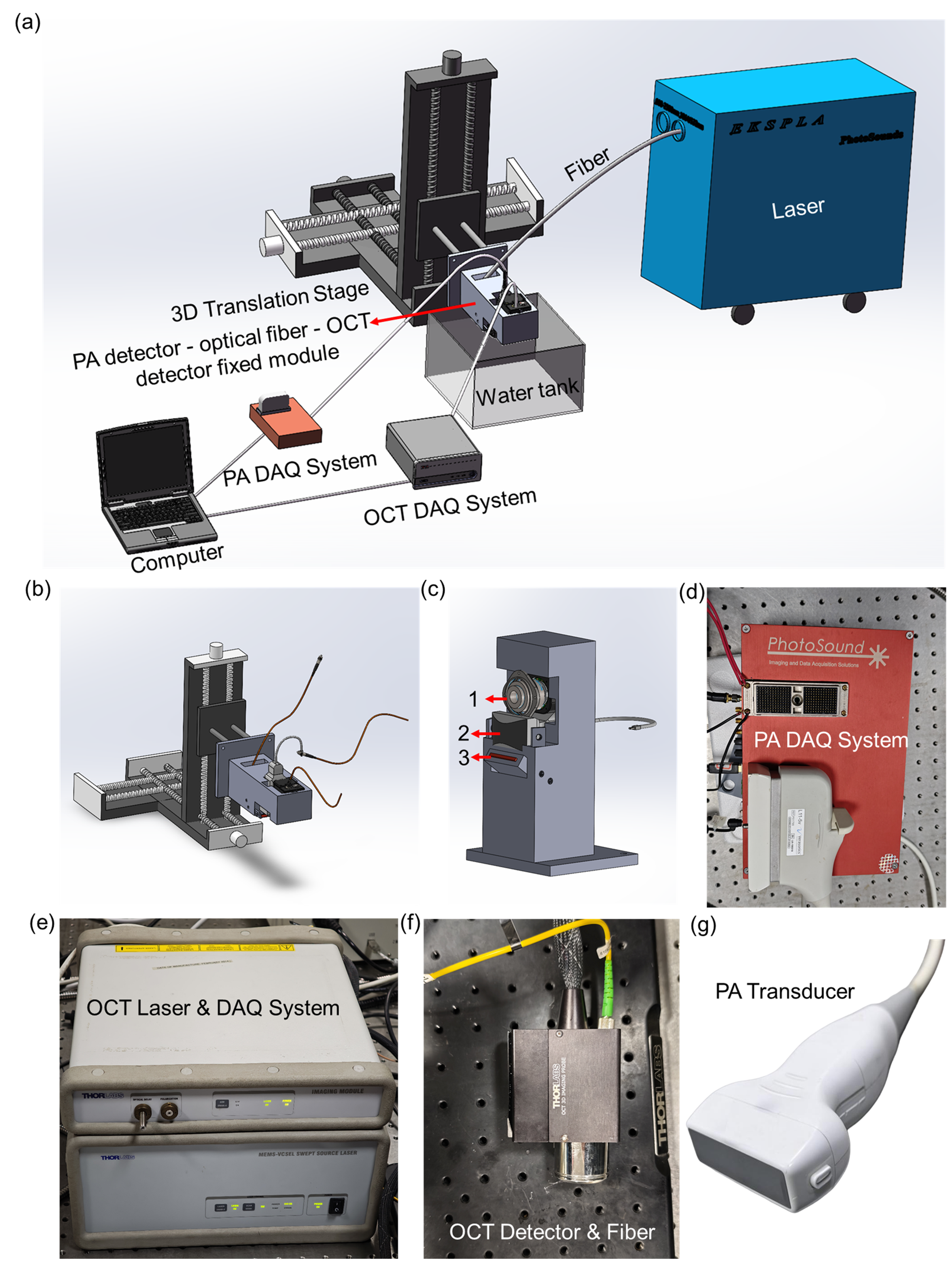
Figure 1. System overview. (a) Schematic of the large-field PA–OCT dual-modal imaging system. (b) Three-dimensional translation stage for montage scanning. (c) Rigid mounting assembly: 1-OCT head, 2-ultrasound probe (PA detector), 3-fiber bundle. (d) Multi-channel PA data acquisition system. (e) OCT light source and acquisition system. (f) OCT detection unit (detector and fiber). (g) Linear-array ultrasound probe.

Figure 1a presents the overall system configuration and the coordination of the OCT and PA acquisition modules. Figure 1b shows the three-dimensional motorized translation stage used for large-field scanning. The stage provides a travel range of 150 mm along each axis, with a nominal positioning resolution of 1.25 μm and repeatability better than 5 μm. Figure 1c shows the rigid mounting assembly, in which the OCT scanning head, linear-array ultrasound transducer, and rectangular photoacoustic excitation fiber bundle are mechanically fixed relative to one another. This common mechanical platform preserves their relative poses during medium exchange and large-range scanning. After an initial spatial calibration, the resulting coordinate transformation can therefore be reused for subsequent acquisitions without feature-based post-registration.

Figure 1d shows the multi-channel PA data-acquisition system used for 128-channel signal reception, amplification, filtering, and digitization. Figure 1e shows the swept-source OCT light-source and acquisition system, Figure 1f presents the OCT detection unit, and Figure 1g shows the linear-array ultrasound transducer used for PA detection.

The large-field acquisition strategy combines internal OCT scanning with programmed translation-stage positioning. The stage-defined nominal coordinate range was 30 mm × 30 mm. OCT data were acquired as a 3 × 3 montage of nine approximately 10 mm × 10 mm × 2 mm sub-volumes. Adjacent OCT sub-fields were acquired with approximately 10% overlap (~1.0 mm) to provide shared image content for montage assembly. Each OCT sub-volume required approximately 15 s for image acquisition and approximately 30 s for data storage. Thus, acquisition of all nine OCT sub-volumes required approximately 2.25 min, while data storage required approximately 4.5 min, corresponding to approximately 6.8 min for OCT acquisition and storage in total.

For PA imaging, the 128-element linear-array transducer covered the lateral dimension along the array direction, while the translation stage scanned along the perpendicular direction. A nominal step interval of 0.05 mm was used over 600 translation steps, corresponding to a nominal scan length of 30 mm. A complete PA scan required approximately 40 s.

The system employed a sequential medium-separation workflow. OCT imaging was first performed in air. Deionized water was subsequently introduced for acoustic coupling, requiring approximately 1 min, followed by approximately 0.5 min of stabilization before PA acquisition. After PA imaging, water removal required approximately 1.5 min. The complete OCT–PA acquisition and medium-exchange procedure therefore required approximately 10.4 min, excluding OCT montage processing and subsequent offline image processing. Throughout this procedure, the phantom remained mechanically fixed on the same sample holder; no manual repositioning was performed during medium exchange, and no visually detectable movement or deformation was observed.

Following acquisition, the PA dataset was mapped to the OCT en face coordinate system using the stored two-dimensional affine transformation. The present implementation therefore establishes two-dimensional en face coordinate correspondence between the OCT and PA datasets rather than full three-dimensional volumetric co-registration.

2.2. Photoacoustic Imaging Methodology

Photoacoustic imaging is based on the photoacoustic effect: pulsed laser light absorbed by tissue generates thermoelastic expansion and subsequent broadband ultrasound emission, which is detected by an ultrasound transducer to form images reflecting optical absorption distribution [6,25]. In this system, a Nd:YAG-pumped OPO laser (EKSPLA, Vilnius, Lithuania) with a repetition rate of 20 Hz, a pulse width of 3–5 ns, and a pulse energy of 200 mJ provides excitation with a tunable output range of 660–2300 nm, supplemented by fixed wavelengths at 532 nm and 1064 nm. The output is delivered through a rectangular fiber bundle (NA = 0.25, 20 mm × 1 mm aperture) to produce a line-shaped beam matching the 128-element linear-array ultrasound probe (L11-5v, Verasonics, Inc., Kirkland, WA, USA) with a center frequency of 8 MHz and an active detection area of 45 × 10 mm².The 128-channel acquisition system (PhotoSound Technologies, Inc., Houston, TX, USA) digitizes signals at 40 MS/s with 12-bit resolution, featuring programmable gain from 14 to 42 dB and a 75 kHz-25 MHz band-pass filter. Maximum amplitude projection (MAP) images were reconstructed from the 3D photoacoustic data.

For all phantom experiments, including the pencil-lead and thin-hair-target experiments, the excitation wavelength was set to 660 nm. The pulse energy measured at the fiber-bundle output was approximately 4.3 mJ. Based on the nominal output aperture of 20 mm × 1 mm, the estimated fluence at the fiber-bundle output was approximately 21.5 mJ/cm². At each scanning position, two consecutive laser-induced PA signal frames were acquired and averaged on a channel-by-channel basis before image reconstruction. The 128-channel signals were reordered according to a predefined channel-mapping table, and the temporal mean of each channel was subtracted to remove the DC offset. PA cross-sectional images were reconstructed using a time-domain delay-and-sum algorithm with an assumed speed of sound of 1495 m/s and a temporal sampling interval of 0.025 μs. The magnitude images were obtained by taking the absolute value of the reconstructed PA amplitude. The sequential cross-sectional images were assembled into a three-dimensional PA dataset, from which maximum-amplitude-projection images were subsequently generated.

2.3. Optical Coherence Tomography Methodology

Optical coherence tomography uses low-coherence interferometry to detect depth-resolved backscattered optical signals and reconstruct cross-sectional structural information [1,26]. Our swept-source OCT module (SL1310V1-10048, Thorlabs, Inc., Newton, NJ, USA) employs a MEMS-VCSEL swept-source laser with a central wavelength of 1300 nm and a sweep bandwidth of approximately 100 nm (full width at half maximum >97 nm). The output power incident on the sample is approximately 25 mW, and the system operates at an A-scan rate of 100 kHz. A dual-balanced photodetector and a 12-bit, 500 MS/s data acquisition card are used for signal detection and digitization.

Beam scanning and focusing were performed using a scan lens (LSM03, Thorlabs, Inc., Newton, NJ, USA) designed for the 1250–1380 nm wavelength range, with an effective focal length (EFL) of 36 mm. The nominal axial and lateral resolutions of the OCT system in air were approximately 12 μm and 22–25 μm, respectively, and the maximum axial ranging depth in air was approximately 12 mm. Interference signals acquired by the balanced detector were processed using Fourier-domain reconstruction to obtain depth-resolved A-lines, from which B-scans and three-dimensional OCT volumes were generated. En face projection images were subsequently calculated from the reconstructed OCT volumes.

To quantitatively evaluate the influence of water coupling under the present experimental geometry, paired OCT measurements were performed under air and water conditions while maintaining the same optical-power setting, scan parameters, detector gain, display settings, and target configuration. For the water-coupled measurements, the water container had a total water depth of approximately 30 mm. The front surface of the OCT scan lens was positioned approximately 28 mm above the water surface, while the pencil-lead target was positioned approximately 23 mm below the water surface, corresponding to a physical water path of approximately 23 mm along the OCT beam.

The air–water comparison was repeated for five paired measurements. Displayed OCT peak levels were extracted using the same analysis procedure for both conditions. The resulting quantitative comparison is presented in Section 3.1. Because the measured signal reduction depends on the water-path length, optical configuration, and OCT acquisition conditions, it was interpreted as a system-specific comparison under the present experimental geometry rather than as a universal attenuation characteristic of water.

2.4. Experimental Setup

Pencil-lead phantoms were used for the principal system-validation experiments because graphite provides strong optical absorption for PA imaging, while the pencil surface and surrounding wood matrix provide distinct structural features for OCT imaging. The phantoms were mechanically fixed to the same sample holder throughout the sequential OCT–PA acquisition procedure. No manual repositioning was performed during water introduction, PA acquisition, or water removal, and no visually detectable movement or deformation of the phantom was observed during medium exchange.

Two types of phantom experiments were performed. First, pencil-lead targets were used to evaluate the influence of water coupling on OCT signal level and to demonstrate the complementary structural and absorption contrasts provided by OCT and PA imaging. Second, a 5 × 5 dual-modal landmark phantom containing 25 spatially distributed pencil-lead targets was used for quantitative evaluation of the coordinate-mapping performance over the large field of view.

OCT imaging was performed first under air coupling. Deionized water was subsequently introduced for PA imaging while the phantom remained fixed on the sample holder. The OCT and PA datasets were expressed in their respective physical coordinate systems and subsequently related using a stored two-dimensional affine transformation. After transformation, the PA maximum-amplitude-projection image was resampled onto the OCT en face coordinate grid. No image-feature-based post-registration, landmark optimization, or iterative correction was applied after acquisition. All quantitative image processing and registration analyses were performed using MATLAB R2022b (The MathWorks, Inc., Natick, MA, USA).

2.5. Quantitative Registration and Repeatability Evaluation

To quantitatively evaluate the hardware-based coordinate-locking strategy, a 5 × 5 landmark phantom containing 25 dual-modal pencil-lead targets was imaged using both OCT and PA over the large-field coordinate range. The targets were numbered row-wise from P01 to P25. Their center coordinates were independently identified in the OCT en face and PA maximum-amplitude-projection images and converted from image-pixel coordinates to physical coordinates in millimeters.

To separate transformation estimation from performance evaluation, nine spatially distributed landmarks—P02, P04, P06, P10, P13, P16, P20, P22, and P24—were predefined as calibration landmarks. Only these nine landmarks were used to estimate the two-dimensional affine transformation from the PA coordinate system to the OCT en face coordinate system. The remaining 16 landmarks—P01, P03, P05, P07, P08, P09, P11, P12, P14, P15, P17, P18, P19, P21, P23, and P25—were completely excluded from transformation estimation and were reserved for independent validation.

A two-dimensional affine transformation T was estimated exclusively from the nine calibration landmarks. After applying the transformation to each validation landmark, the residual displacement components were calculated as

$$\begin{gathered} \Delta xi={xi}^{PA\to OCT}-{xi}^{OCT} \\ \Delta yi={yi}^{PA\to OCT}-{yi}^{OCT} \end{gathered}$$

and the two-dimensional registration error was defined as

$$ei=\sqrt{{(\Delta xi)}^2+{(\Delta yi)}^2}$$

Calibration fitting residuals were calculated separately using the nine calibration landmarks, whereas registration performance was evaluated using only the 16 withheld validation landmarks. The mean error, standard deviation, root-mean-square error (RMSE), maximum error, and 95th-percentile error were calculated from the validation measurements. In addition, a full-field residual-error vector map was generated to visualize the magnitude and spatial direction of the registration errors across the field of view.

To evaluate the repeatability of the one-time calibration during repeated medium switching, five additional OCT–PA acquisition cycles were performed. The affine transformation obtained from the initial calibration was kept fixed throughout all five cycles, and no recalibration was performed. For each cycle, the same 16 validation landmarks were independently localized in the OCT and PA datasets, and their two-dimensional registration errors were calculated after application of the fixed transformation. A total of 80 validation measurements (16 landmarks × 5 cycles) were therefore included in the repeatability analysis. No feature-based post-registration or landmark-based correction was performed in any repeatability cycle.

2.6. Cross-Sectional Profile Analysis

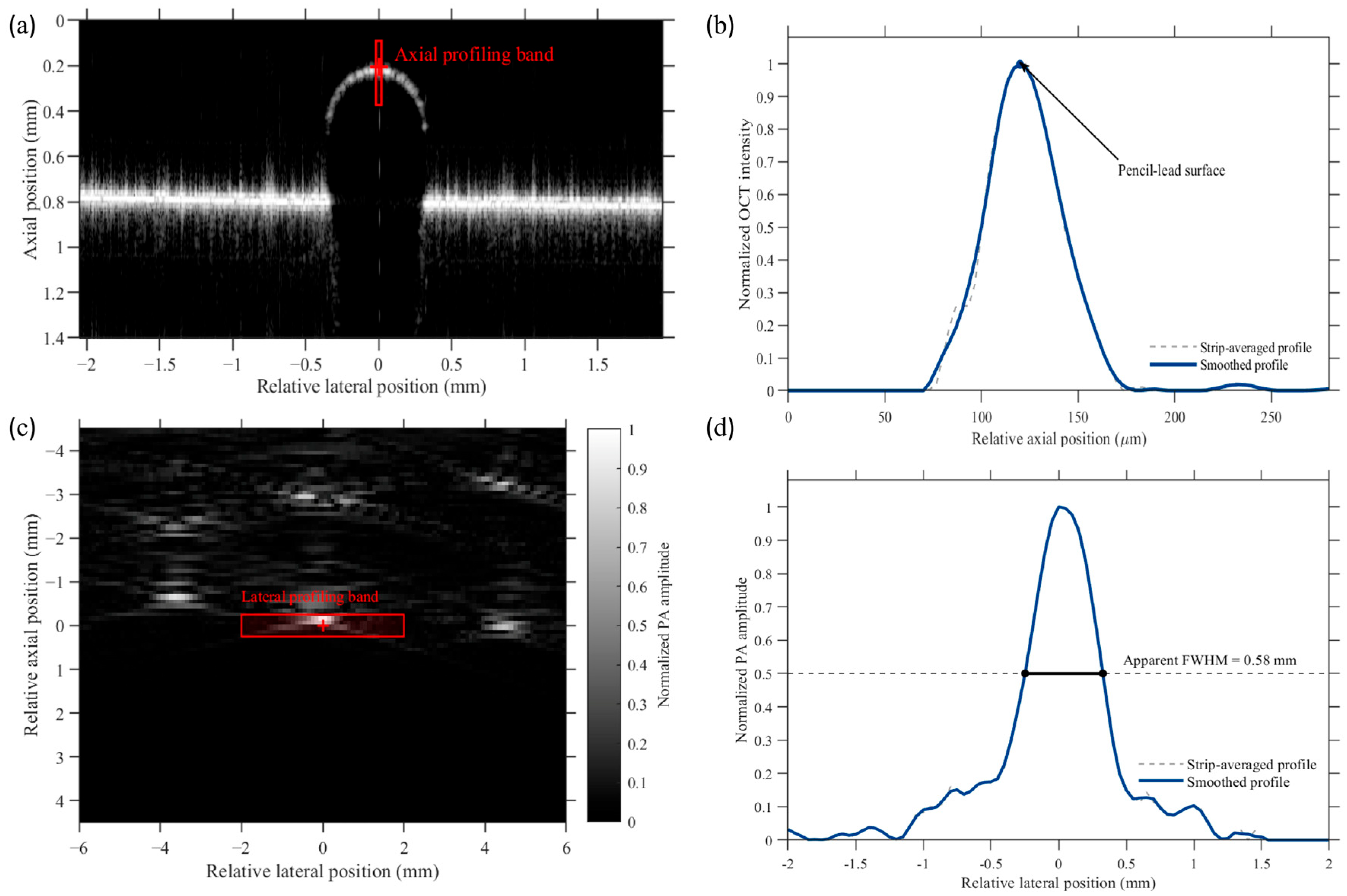
To characterize the complementary cross-sectional responses of a representative 0.5 mm diameter pencil-lead target, corresponding OCT and PA cross-sections were selected using the common stage-coordinate mapping. For OCT analysis, a narrow vertical profiling band centered on the apex of the pencil-lead surface was selected from the reconstructed B-scan image. The image intensities within the profiling band were averaged laterally to obtain a one-dimensional axial intensity profile. The background level was estimated from the pre-surface region and subtracted from the entire profile, after which negative values were set to zero. The background-corrected profile was normalized to its maximum value. An 11-point Savitzky–Golay filter was then applied to generate a smoothed curve for visualization and surface-peak identification, while the original normalized strip-averaged profile was retained for comparison. The axial coordinate was converted using a calibration factor of 3.33 μm per pixel in air.

For PA analysis, a rectangular profiling band covering the representative target was selected from the reconstructed cross-sectional image. The PA amplitudes within the selected region were averaged along the axial direction to obtain a one-dimensional lateral profile, which was subsequently normalized to its maximum value. The apparent full width at half maximum (FWHM) was determined from the two intersections between the normalized profile and the 0.5-amplitude level using linear interpolation. Because the pencil lead had a finite nominal diameter of 0.5 mm, the resulting FWHM was interpreted only as the apparent image-domain width of the finite absorber. It was not used to characterize the intrinsic PA spatial resolution; a dedicated thin-hair-target resolution experiment was performed separately as described in Section 2.7.

2.7. PA Spatial-Resolution Measurement Method

A separate experiment using six thin hair targets was performed to characterize the spatial response of the PA subsystem independently of the 0.5 mm pencil-lead phantom. PA B-scan data were acquired from the hair targets using the same PA acquisition and reconstruction framework described in Section 2.2.

For resolution analysis, the reconstructed PA B-scans used a lateral grid spacing of 0.05 mm and an axial grid spacing of 0.01 mm. The finer axial reconstruction interval was used to provide denser numerical sampling of the axial response profile and does not represent an improvement in the physical resolution of the imaging system.

For each hair target, the peak-response location was identified in the reconstructed PA B-scan. A one-dimensional lateral profile was extracted through the target response along the lateral direction, and an axial profile was extracted through the corresponding response along the depth direction. Each profile was normalized to its maximum amplitude.

A Gaussian function was fitted to the principal response peak of each normalized profile, and the full width at half maximum (FWHM) of the fitted curve was used as the spatial-response metric. Lateral and axial FWHM values were independently obtained for all six hair targets. The resulting resolution estimates were reported as mean ± standard deviation (n = 6). The hair targets were used as thin absorbing targets for FWHM-based spatial-response characterization; because their diameters were not independently measured in the present study, no target-size deconvolution was applied.

3. Results

3.1. Necessity of Medium Separation: Quantitative OCT Air–Water Comparison

To quantitatively evaluate the influence of water coupling on the OCT signal under the present experimental geometry, paired measurements were performed in air and deionized water using the same acquisition parameters, optical-power setting, detector gain, display settings, and target configuration. During the water-coupled measurements, the physical water path from the water surface to the pencil-lead target was approximately 23 mm.

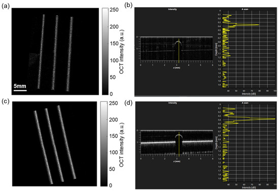
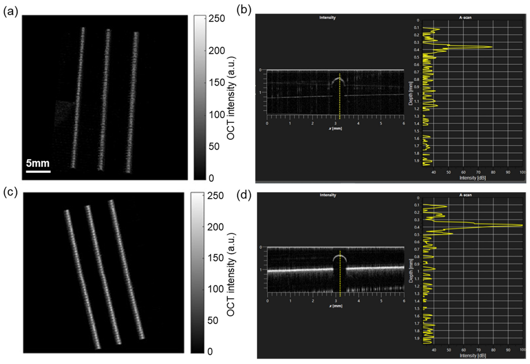
Representative OCT images under the two coupling conditions are shown in Figure 2. Water immersion substantially reduced the visibility of superficial target features compared with imaging in air. This qualitative observation was consistent with the quantitative peak-level measurements.

Figure 2. Quantitative comparison of OCT imaging under water and air conditions. (a) Three-dimensional OCT reconstruction of the pencil-lead phantom in deionized water, showing substantial loss of superficial detail. (b) Representative cross-sectional OCT signal in water, with a displayed peak level of approximately 80 dB. (c) Three-dimensional OCT reconstruction of the same phantom in air, showing improved visualization of surface features. (d) Representative cross-sectional OCT signal acquired in air. Across five paired measurements, the displayed OCT peak level decreased from 98.4 ± 1.5 dB in air to 79.4 ± 1.8 dB in water, corresponding to a mean reduction of 19.0 ± 1.4 dB under the present experimental geometry.

Across five paired measurements, the displayed OCT peak levels were 99, 98, 100, 99, and 96 dB in air, compared with 78, 81, 81, 80, and 77 dB in water, respectively. The mean peak level decreased from 98.4 ± 1.5 dB in air to 79.4 ± 1.8 dB in water. The corresponding paired reductions ranged from 17 to 21 dB, with a mean reduction of 19.0 ± 1.4 dB (mean ± SD, n = 5).

These results support the use of temporal medium separation in the present system, in which OCT imaging is performed in air while water coupling is introduced only for PA acquisition. The measured reduction should be interpreted as specific to the present 23 mm water path, optical geometry, and system settings rather than as a universal attenuation value for 1300 nm OCT imaging.

3.2. Single-Target Cross-Sectional Characterization

To illustrate the complementary cross-sectional information provided by OCT and PAI, a representative 0.5 mm-diameter pencil-lead target was selected from the phantom array. Corresponding OCT and PA cross-sections were identified using the common stage-coordinate mapping.

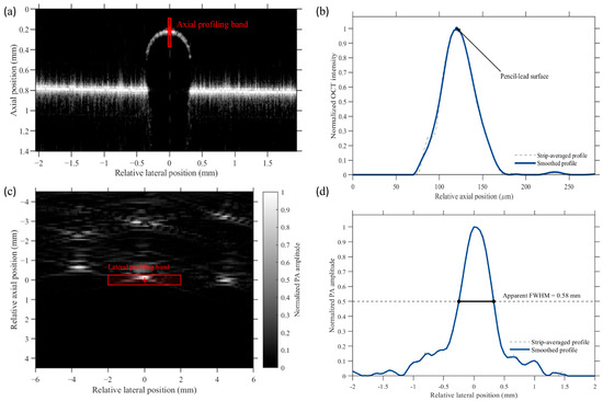
The OCT B-scan in Figure 3a shows a localized superficial response at the upper boundary of the pencil-lead target. The red solid band indicates the region used for axial profile extraction. As shown in Figure 3b, both the strip-averaged profile and the smoothed profile exhibit a distinct peak at the superficial target boundary, demonstrating the sensitivity of OCT to the surface structural interface.

Figure 3. Cross-sectional characterization of a representative 0.5 mm-diameter pencil-lead target using OCT and PA imaging. (a) OCT B-scan showing the superficial response of the target, with the axial profiling band indicated by the red solid box. (b) Normalized axial OCT intensity profiles. The gray dashed curve and blue solid curve represent the strip-averaged and smoothed profiles, respectively. (c) Local PA cross-sectional image of the same physical target, with the lateral profiling band indicated by the red solid box. (d) Normalized lateral PA amplitude profile, showing an apparent FWHM of 0.58 mm. The OCT axial profile and PA lateral profile describe different spatial directions and physical contrasts. Therefore, the apparent PA FWHM represents the image-domain width of the finite-size target and is not interpreted as the intrinsic PA spatial resolution or as a direct comparison with the OCT resolution.

The PA cross-sectional image in Figure 3c visualizes the optical absorption distribution associated with the same physical target. The red rectangular band indicates the region used to extract the lateral amplitude profile. The normalized profile in Figure 3d exhibits an apparent FWHM of 0.58 mm, which is close to the nominal diameter of the 0.5 mm pencil lead but also includes broadening introduced by the imaging response and reconstruction process.

These measurements demonstrate that OCT and PA imaging provide different but complementary descriptions of the same target. OCT primarily characterizes the superficial structural response along the axial direction, whereas PA imaging visualizes the lateral distribution of optical absorption. Because the two profiles represent different spatial directions and physical contrasts, their peak positions and widths were not used to quantify intermodal registration or directly compare intrinsic spatial resolution. Quantitative registration performance is evaluated independently in Section 3.4, while dedicated PA spatial-resolution characterization using thin hair targets is presented in Section 3.5.

3.3. Large-Field Dual-Modal Imaging

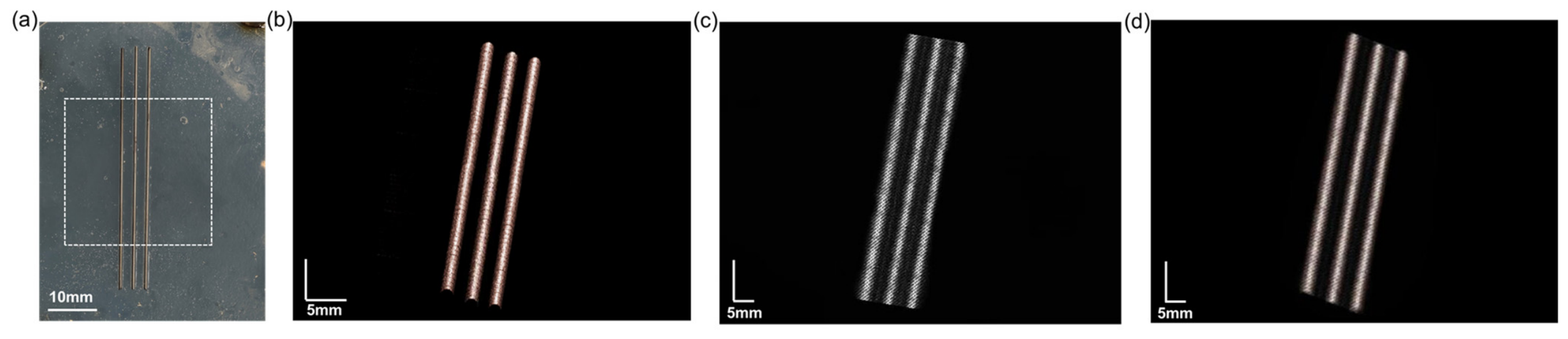
Large-field dual-modal imaging was first demonstrated using the pencil-lead phantom array. The phantom was sequentially imaged using OCT in air and PA imaging after introduction of deionized water. The imaging region was defined within the common stage-coordinate range used by both modalities.

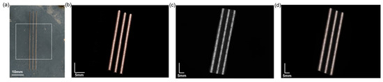
For OCT imaging, nine approximately 10 mm × 10 mm sub-fields were acquired in a 3 × 3 arrangement with approximately 10% overlap between adjacent fields and combined to generate the large-field en face representation. As shown in Figure 4b, OCT visualized superficial wood-grain patterns and graphite-related surface features with high structural detail.

Figure 4. Large-field dual-modal phantom imaging. (a) Photograph of the pencil-lead phantom array, with the scanned region indicated by the dashed rectangle. (b) OCT en face image acquired in air using montage scanning, showing superficial wood-grain patterns and graphite-related surface features. (c) PA maximum-amplitude-projection image acquired with water coupling, showing absorption contrast from the graphite components. (d) Overlay of the OCT and PA images after application of the one-time coordinate transformation. The overlay demonstrates qualitative spatial correspondence over the common field of view without feature-based post-registration.

After OCT acquisition, deionized water was introduced for acoustic coupling without repositioning the phantom. The PA system subsequently scanned the corresponding region using 600 translation steps at a nominal interval of 0.05 mm. The resulting PA maximum-amplitude-projection image in Figure 4c provided absorption-based contrast from the graphite components.

After application of the stored two-dimensional affine transformation, the PA dataset was mapped to the OCT en face coordinate grid. Corresponding structures occupied visually consistent locations in the transformed overlay shown in Figure 4d. No image-feature-based post-registration, landmark optimization, or iterative correction was applied after acquisition.

Figure 4 therefore provides a qualitative visualization of large-field dual-modal correspondence under modality-specific coupling conditions. Quantitative registration accuracy and repeatability were evaluated independently using the 25-landmark phantom, as described in Section 3.4.

3.4. Quantitative Registration Accuracy and Medium-Switching Repeatability

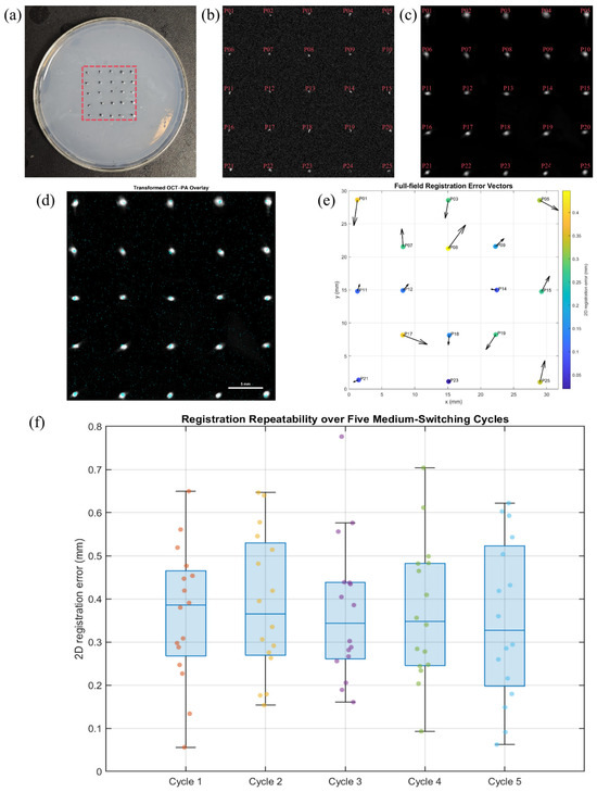
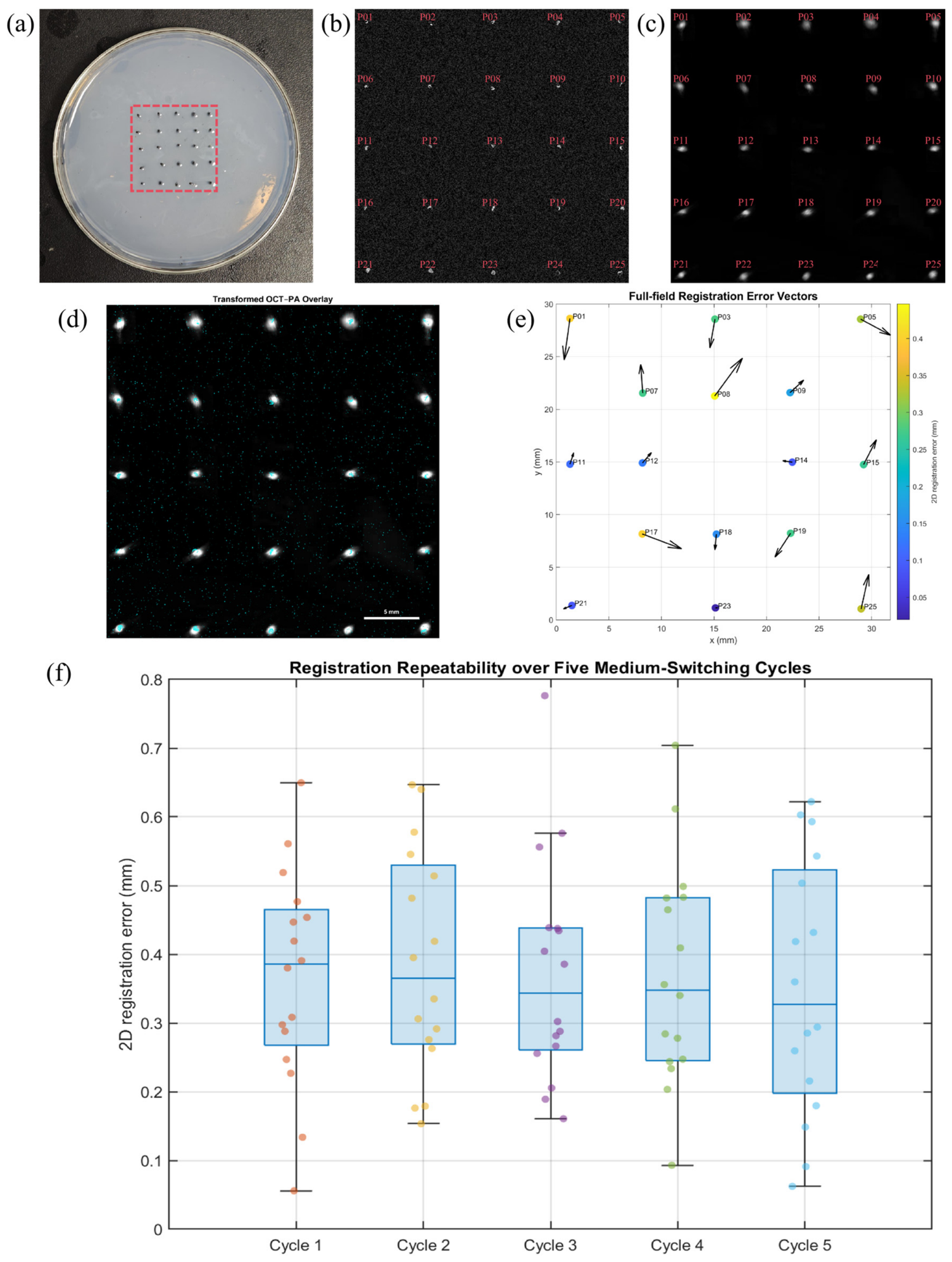
To quantitatively evaluate the hardware-based coordinate-locking strategy, a 5 × 5 phantom containing 25 dual-modal landmarks was imaged using both OCT and PA. Nine spatially distributed landmarks were used exclusively for affine calibration, while the remaining 16 landmarks were excluded from transformation estimation and reserved for independent validation (Figure 5a–c).

Figure 5. Quantitative evaluation of OCT–PA coordinate mapping and medium-switching repeatability. (a) Photograph of the 5 × 5 dual-modal landmark phantom. (b) OCT en face image with landmarks P013–P25. (c) PA maximum-amplitude-projection image with corresponding landmarks. Nine predefined landmarks (P02, P04, P06, P10, P13, P16, P20, P22, and P24) were used exclusively for affine calibration, while the remaining 16 landmarks were reserved for independent validation. (d) OCT–PA overlay after application of the calibrated two-dimensional affine transformation. (e) Full-field registration-error vector map for the 16 validation landmarks; vector lengths are magnified 10-fold for visualization, whereas color indicates the measured two-dimensional error magnitude. (f) Registration-error distributions over five repeated medium-switching cycles using the fixed initial affine transformation. Each cycle contains 16 validation landmarks, and no recalibration or feature-based post-registration was performed.

For the nine calibration landmarks, the mean fitting residual was 0.233 mm, with an RMSE of 0.249 mm and a maximum residual of 0.351 mm. These values characterize the fitting consistency of the affine transformation itself and were analyzed separately from the withheld validation landmarks.

After applying the calibrated transformation to the 16 independent validation landmarks, the mean two-dimensional registration error was 0.235 ± 0.128 mm, with an RMSE of 0.266 mm. The maximum observed validation error was 0.446 mm, and the 95th-percentile error was 0.413 mm. All 16 validation landmarks exhibited registration errors below 0.5 mm in the initial full-field validation experiment.

Figure 5d shows the transformed OCT–PA overlay obtained using the calibration derived only from the nine designated calibration landmarks. The full-field error-vector map in Figure 5e illustrates the magnitude and direction of the residual registration errors at the 16 independent validation landmarks. The residuals were distributed across the field rather than being evaluated only near the calibration region, providing a field-wide assessment of the two-dimensional coordinate mapping.

The stability of the one-time calibration was further evaluated over five additional medium-switching cycles. The original affine transformation was kept fixed throughout all five cycles, and no recalibration or feature-based post-registration was performed. The mean two-dimensional registration errors for Cycles 1–5 were 0.366, 0.387, 0.372, 0.371, and 0.351 mm, respectively (Figure 5f).

Across all 80 validation measurements obtained from the five cycles, the overall registration error was 0.369 ± 0.163 mm, with an RMSE of 0.404 mm, a 95th-percentile error of 0.643 mm, and a maximum error of 0.776 mm. Importantly, the cycle-wise mean errors remained within a relatively narrow range and showed no progressive increase over repeated medium switching. These results demonstrate that the initial two-dimensional coordinate transformation remained reusable over repeated sequential OCT–PA acquisition cycles under the present phantom conditions.The quantitative registration performance for calibration fitting, initial independent validation, and five-cycle repeatability is summarized in Table 1.

Table 1. Quantitative registration performance.

Metric	Calibration Fitting	Initial Independent Validation	Five-Cycle Repeatability
Number of measurements	9	16	80
Mean error (mm)	0.233	0.235	0.369
SD (mm)	-	0.128	0.163
RMSE (mm)	0.249	0.266	0.404
Maximum error (mm)	0.351	0.446	0.776
P95 error (mm)	-	0.413	0.643

Table 1. Quantitative registration performance.

Metric	Calibration Fitting	Initial Independent Validation	Five-Cycle Repeatability
Number of measurements	9	16	80
Mean error (mm)	0.233	0.235	0.369
SD (mm)	-	0.128	0.163
RMSE (mm)	0.249	0.266	0.404
Maximum error (mm)	0.351	0.446	0.776
P95 error (mm)	-	0.413	0.643

Calibration fitting metrics were calculated from the nine landmarks used to estimate the affine transformation. Independent validation metrics were calculated only from landmarks excluded from transformation estimation. Five-cycle repeatability metrics summarize 80 validation measurements acquired without recalibration.

3.5. PA Spatial-Resolution Characterization

A dedicated thin-hair-target experiment was performed to characterize the spatial response of the PA subsystem independently of the finite 0.5 mm pencil-lead target used in Figure 3. Six hair targets were independently imaged and analyzed.

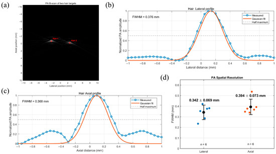
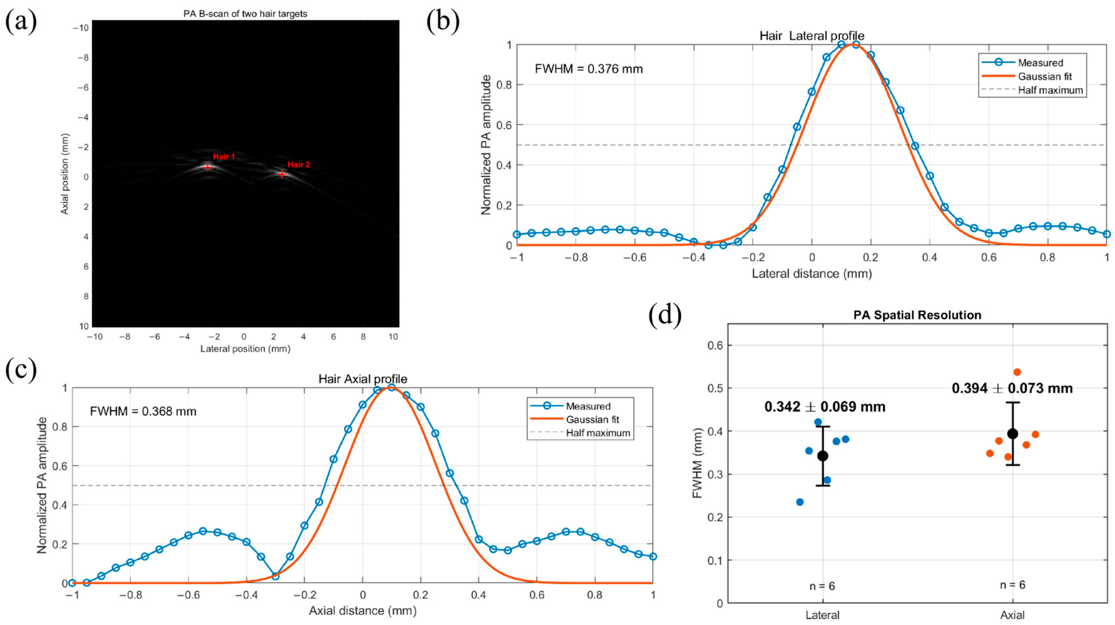
Representative reconstructed PA B-scan images and normalized profile measurements are shown in Figure 6. Gaussian fitting was applied to the principal lateral and axial response peaks, and the corresponding FWHM values were calculated for each target.

Figure 6. FWHM-based spatial-resolution characterization of the PA subsystem using thin hair targets. (a) Representative PA B-scan of thin hair targets, with profile-extraction locations indicated. (b) Representative normalized lateral PA profile and Gaussian fit. (c) Representative normalized axial PA profile and Gaussian fit. (d) Summary of lateral and axial FWHM values obtained from six independently measured hair targets. Individual measurements are shown together with mean ± SD. The mean lateral and axial FWHM values were 0.342 ± 0.069 mm and 0.394 ± 0.073 mm, respectively.

The six lateral FWHM values were 0.235, 0.354, 0.421, 0.286, 0.376, and 0.381 mm, yielding a mean lateral FWHM of 0.342 ± 0.069 mm. The corresponding axial FWHM values were 0.348, 0.377, 0.340, 0.537, 0.368, and 0.392 mm, yielding a mean axial FWHM of 0.394 ± 0.073 mm.

Thus, under the present acquisition and reconstruction conditions, the FWHM-based PA spatial-response estimates were 0.342 ± 0.069 mm laterally and 0.394 ± 0.073 mm axially (mean ± SD, n = 6). These measurements provide a more appropriate characterization of the PA spatial response than the apparent 0.58 mm width obtained from the finite 0.5 mm pencil-lead target. Because the hair diameters were not independently measured, these values are reported as FWHM-based spatial-resolution estimates without target-size deconvolution.

4. Discussion

This study presents a large-field photoacoustic–OCT dual-modal imaging workflow based on temporal medium separation and hardware-based coordinate locking. The revised experiments quantitatively evaluate the influence of water coupling on OCT, the accuracy and repeatability of two-dimensional OCT–PA coordinate mapping, and the spatial response of the PA subsystem.

The air–water comparison supports the use of temporal medium separation in the present system. With an approximately 23 mm physical water path and otherwise unchanged OCT acquisition settings, the displayed OCT peak level decreased from 98.4 ± 1.5 dB in air to 79.4 ± 1.8 dB in water, corresponding to a mean reduction of 19.0 ± 1.4 dB across five paired measurements. This reduction is specific to the present optical geometry and acquisition conditions and should not be interpreted as a universal attenuation value for water. Nevertheless, it demonstrates that performing OCT in air while introducing water only for PA acquisition is advantageous for the current system.

Quantitative registration experiments further validate the hardware-based coordinate-locking strategy. Nine landmarks were used exclusively for affine calibration, while 16 additional landmarks were withheld for independent validation. The mean calibration residual was 0.233 mm, whereas the independent validation error was 0.235 ± 0.128 mm, with an RMSE of 0.266 mm and a maximum error of 0.446 mm. The full-field error-vector map also revealed the spatial distribution of the residual mapping errors. These results provide quantitative evidence for sub-millimeter two-dimensional coordinate correspondence beyond the qualitative overlay shown in the large-field phantom experiment.

The one-time transformation also remained reasonably stable during repeated medium switching. Over five additional OCT–PA acquisition cycles without recalibration, the mean two-dimensional errors ranged from 0.351 to 0.387 mm. Across 80 validation measurements, the overall error was 0.369 ± 0.163 mm, with an RMSE of 0.404 mm, a 95th-percentile error of 0.643 mm, and a maximum error of 0.776 mm. Although these errors were larger than those in the initial validation, no progressive deterioration was observed across the five cycles. The present approach should therefore be interpreted as providing sub-millimeter two-dimensional en face coordinate mapping, rather than exact point-to-point or three-dimensional volumetric co-registration.

The dedicated thin-hair experiment also provides a more appropriate characterization of the PA subsystem than the previous 0.5 mm pencil-lead measurement. Using six hair targets, the FWHM-based spatial-resolution estimates were 0.342 ± 0.069 mm laterally and 0.394 ± 0.073 mm axially. Because the hair diameters were not independently measured, these values are reported as experimental FWHM-based resolution estimates without target-size deconvolution. The earlier 0.58 mm pencil-lead FWHM should therefore be regarded only as the apparent image-domain width of a finite absorber.

Several limitations remain. The present work is restricted to rigid phantom experiments and two-dimensional en face registration; biological tissues may introduce deformation, motion, and more complex depth-dependent correspondence. Medium exchange was performed manually, although the phantom remained fixed without manual repositioning or visually detectable deformation. The complete acquisition and medium-exchange procedure required approximately 10.4 min, excluding offline processing. Future work should therefore focus on automated medium handling, three-dimensional registration, resolution measurements using targets of known dimensions, multi-wavelength PA imaging, and validation in ex vivo and in vivo tissues. Within these limitations, the present results support the proposed method as a phantom-based technical validation of reusable OCT–PA coordinate mapping under modality-specific coupling conditions.

5. Conclusions

We developed a large-field photoacoustic–OCT dual-modal imaging system based on temporal medium separation and hardware-based coordinate locking. OCT acquisition in air and PA acquisition under water coupling allowed the two modalities to operate under their respective preferred coupling conditions. Under the present experimental geometry, the OCT peak level decreased by 19.0 ± 1.4 dB in water relative to air across five paired measurements. Quantitative validation using a 25-landmark phantom demonstrated a mean two-dimensional registration error of 0.235 ± 0.128 mm for 16 independent validation landmarks, while five additional medium-switching cycles performed without recalibration yielded an overall error of 0.369 ± 0.163 mm. Dedicated thin-hair measurements further yielded FWHM-based PA spatial-resolution estimates of 0.342 ± 0.069 mm laterally and 0.394 ± 0.073 mm axially. These results demonstrate reproducible sub-millimeter two-dimensional en face OCT–PA coordinate mapping without feature-based post-registration. The present study should be regarded as a phantom-based technical validation, and future work will focus on automated medium switching, three-dimensional registration, and validation using ex vivo and in vivo biological tissues.

References

- Huang, D.; Swanson, E.A.; Lin, C.P.; Schuman, J.S.; Stinson, W.G.; Chang, W.; Hee, M.R.; Flotte, T.; Gregory, K.; Puliafito, C.A.; et al. Optical coherence tomography. Science 1991, 254, 1178–1181. [Google Scholar] [CrossRef] [Scilit] [PubMed]
- Drexler, W.; Liu, M.; Kumar, A.; Kamali, T.; Unterhuber, A.; Leitgeb, R.A. Optical coherence tomography today: Speed, contrast, and multimodality. J. Biomed. Opt. 2014, 19, 071412. [Google Scholar] [CrossRef] [Scilit] [PubMed]
- Chen, S.; Potsaid, B.; Li, Y.; Lin, J.; Hwang, Y.; Moult, E.M.; Zhang, J.; Huang, D.; Fujimoto, J.G. High speed, long range, deep penetration swept source OCT for structural and angiographic imaging of the anterior eye. Sci. Rep. 2022, 12, 992. [Google Scholar] [CrossRef] [Scilit] [PubMed]
- De Boer, J.F.; Hitzenberger, C.K.; Yasuno, Y. Polarization sensitive optical coherence tomography-a review. Biomed. Opt. Express 2017, 8, 1838–1873. [Google Scholar] [CrossRef] [Scilit] [PubMed]
- Podoleanu, A.G. Optical coherence tomography. J. Microsc. 2012, 247, 209–219. [Google Scholar] [CrossRef] [Scilit] [PubMed]
- Wang, L.V.; Hu, S. Photoacoustic tomography: In vivo imaging from organelles to organs. Science 2012, 335, 1458–1462. [Google Scholar] [CrossRef] [Scilit] [PubMed]
- Xia, J.; Yao, J.; Wang, L.V. Photoacoustic tomography: Principles and advances. Electromagn. Waves 2014, 147, 1–22. [Google Scholar] [CrossRef] [Scilit] [PubMed]
- Upputuri, P.K.; Pramanik, M. Recent advances in photoacoustic contrast agents for in vivo imaging. Wiley Interdiscip. Rev. Nanomed. Nanobiotechnol. 2020, 12, e1618. [Google Scholar] [CrossRef] [Scilit] [PubMed]
- Wang, H.; Ma, Y.; Yang, H.; Jiang, H.; Ding, Y.; Xie, H. MEMS ultrasound transducers for endoscopic photoacoustic imaging applications. Micromachines 2020, 11, 928. [Google Scholar] [CrossRef] [Scilit] [PubMed]
- Manwar, R.; Kratkiewicz, K.; Avanaki, K. Overview of ultrasound detection technologies for photoacoustic imaging. Micromachines 2020, 11, 692. [Google Scholar] [CrossRef] [Scilit] [PubMed]
- Chen, Z.; Gezginer, I.; Zhou, Q.; Tang, L.; Deán-Ben, X.L.; Razansky, D. Multimodal optoacoustic imaging: Methods and contrast materials. Chem. Soc. Rev. 2024, 53, 6068–6099. [Google Scholar] [CrossRef] [Scilit] [PubMed]
- Wang, L.V. Multiscale photoacoustic microscopy and computed tomography. Nat. Photonics 2009, 3, 503–509. [Google Scholar] [CrossRef] [Scilit] [PubMed]
- Hale, G.M.; Querry, M.R. Optical constants of water in the 200-nm to 200-μ m wavelength region. Appl. Opt. 1973, 12, 555–563. [Google Scholar] [CrossRef] [Scilit] [PubMed]
- Kou, L.; Labrie, D.; Chylek, P. Refractive indices of water and ice in the 0.65-to 2.5-μm spectral range. Appl. Opt. 1993, 32, 3531–3540. [Google Scholar] [CrossRef] [Scilit] [PubMed]
- Yao, J.; Wang, L.V. Sensitivity of photoacoustic microscopy. Photoacoustics 2014, 2, 87–101. [Google Scholar] [CrossRef] [Scilit] [PubMed]
- Jeon, S.; Kim, J.; Lee, D.; Baik, J.W.; Kim, C. Review on practical photoacoustic microscopy. Photoacoustics 2019, 15, 100141. [Google Scholar] [CrossRef] [Scilit] [PubMed]
- Bondu, M.; Marques, M.; Moselund, P.; Lall, G.; Bradu, A.; Podoleanu, A. Multispectral photoacoustic microscopy and optical coherence tomography using a single supercontinuum source. Photoacoustics 2018, 9, 21–30. [Google Scholar] [CrossRef] [Scilit] [PubMed]
- Chen, Z.; Rank, E.; Meiburger, K.M.; Sinz, C.; Hodul, A.; Zhang, E.; Hoover, E.; Minneman, M.; Ensher, J.; Beard, P.C.; et al. Non-invasive multimodal optical coherence and photoacoustic tomography for human skin imaging. Sci. Rep. 2017, 7, 17975. [Google Scholar] [CrossRef] [Scilit] [PubMed]
- Ding, N.; Jiang, H.; Xiang, B.; Yu, Y.; Ji, C.; Liu, J.; Zhao, Y.; Luan, J.; Yang, Y.; Wang, Y.; et al. Probe fusion all-optic OCT-PAM dual-mode imaging system for biomedical imaging. Photoacoustics 2024, 38, 100631. [Google Scholar] [CrossRef] [Scilit] [PubMed]
- Zafar, M.; Siegel, A.P.; Avanaki, K.; Manwar, R. Skin imaging using optical coherence tomography and photoacoustic imaging: A mini-review. Optics 2024, 5, 248–266. [Google Scholar] [CrossRef] [Scilit]
- Park, J.; Park, B.; Kim, T.Y.; Jung, S.; Choi, W.J.; Ahn, J.; Yoon, D.H.; Kim, J.; Jeon, S.; Lee, D.; et al. Quadruple ultrasound, photoacoustic, optical coherence, and fluorescence fusion imaging with a transparent ultrasound transducer. Proc. Natl. Acad. Sci. USA 2021, 118, e1920879118. [Google Scholar] [CrossRef] [Scilit] [PubMed]
- Shen, B.; Luo, C.; Pang, W.; Jiang, Y.; Wu, W.; Hu, R.; Qu, J.; Gu, B.; Liu, L. Surmounting photon limits and motion artifacts for biological dynamics imaging via dual-perspective self-supervised learning. PhotoniX 2024, 5, 1–24. [Google Scholar] [CrossRef] [Scilit]
- Park, E.; Kim, D.; Ha, M.; Kim, D.; Kim, C. A comprehensive review of high-performance photoacoustic microscopy systems. Photoacoustics 2025, 44, 100739. [Google Scholar] [CrossRef] [Scilit] [PubMed]
- Lin, L.; Hu, P.; Shi, J.; Appleton, C.M.; Maslov, K.; Li, L.; Zhang, R.; Wang, L.V. Single-breath-hold photoacoustic computed tomography of the breast. Nat. Commun. 2018, 9, 2352. [Google Scholar] [CrossRef] [Scilit] [PubMed]
- Beard, P. Biomedical photoacoustic imaging. Interface Focus 2011, 1, 602–631. [Google Scholar] [CrossRef] [Scilit] [PubMed]
- Fercher, A.F.; Drexler, W.; Hitzenberger, C.K.; Lasser, T. Optical coherence tomography-principles and applications. Rep. Prog. Phys. 2003, 66, 239–303. [Google Scholar] [CrossRef] [Scilit]
Disclaimer/Publisher’s Note: The statements, opinions and data contained in all publications are solely those of the individual author(s) and contributor(s) and not of MDPI and/or the editor(s). MDPI and/or the editor(s) disclaim responsibility for any injury to people or property resulting from any ideas, methods, instructions or products referred to in the content. |
© 2026 by the authors. Licensee MDPI, Basel, Switzerland. This article is an open access article distributed under the terms and conditions of the Creative Commons Attribution (CC BY) license.