Time-Resolved Fluorescence of a Two-Level System Using Time-Dependent Variational Method

Abstract

The time-resolved fluorescence spectrum of a driven two-level system is investigated using a time-dependent variational method. We first establish the transient build-up of the Mollow triplet via the Lindblad master equation under the rotating-wave approximation, providing a complete visualization of the spectral evolution from initial turn-on to steady state. To go beyond the perturbative regime, we employ the multiple Davydov D₂ ansatz (multi-D₂), which uses the ${\sigma }_z$ eigenstates as the basis and naturally accommodates arbitrary system–bath coupling types and spectral densities. The multi-D₂ method converges with M = 4 multiplicities in studied cases, outperforming the multi-D₁ ansatz (M = 8) for the ${\sigma }_x$ coupling benchmark. For pure ${\sigma }_z$ (dephasing) coupling under resonant driving, we find that the time-resolved spectrum reveals a distinct fluorescence peak at the Rabi frequency—a signature of dressed-state transitions induced by the dephasing channel that remains hidden in population dynamics. Under mixed ${\sigma }_x$–${\sigma }_z$ coupling, the spectrum exhibits combined features of both Mollow triplet and ${\sigma }_z$-mediated emission. The effects of sub-Ohmic, Ohmic, and super-Ohmic spectral densities are systematically compared. While the resonant spectral weight $J\left({\omega }_0\right)$ governs the overall dissipation rate, a controlled comparison at fixed $J\left({\omega }_0\right)$ reveals that the super-Ohmic regime exhibits an intrinsic shape-dependent suppression of sideband emission under resonant driving, highlighting an asymmetric role of the spectral density exponent in engineering transient fluorescence. Our work establishes the multi-D₂ ansatz as a versatile tool for simulating time-resolved fluorescence in complex bosonic environments.

1. Introduction

Resonance fluorescence—the light scattered by a two-level system (TLS) driven by a resonant or near-resonant coherent field—has been a cornerstone of quantum optics since its theoretical prediction by Mollow [1] and subsequent experimental observation [2]. In the steady-state limit and under strong driving, the fluorescence spectrum exhibits a characteristic three-peak structure known as the Mollow triplet, which has been extensively studied in various physical platforms including natural atoms [3], semiconductor quantum dots [4,5], and superconducting circuits [6,7]. The dressed-state picture provides an intuitive interpretation: the optical drive hybridizes the bare atomic states with the photon field, creating a ladder of dressed states whose dipole-allowed transitions give rise to the three spectral peaks separated by the generalized Rabi frequency [8,9].

Despite this mature understanding of the steady-state spectrum, the transient build-up of the fluorescence signal—i.e., how the Mollow triplet emerges from the initial turn-on of the driving field—has received considerably less attention. Early works by Renaud et al. [10] and Eberly et al. [11] studied the time-dependent spectrum using the physical spectrum approach [12], but these studies were largely confined to the weak-driving and weak-coupling regimes where the rotating-wave approximation (RWA) is valid. More recently, Boström et al. [13] explored time-resolved multiphoton effects in fluorescence spectra using an exact numerical method, revealing four-peak structures and second-harmonic generation in the intermediate-coupling regime. Despite these advances, a comprehensive visualization of the full transient evolution from the initial state to the steady-state Mollow triplet—including the turn-on dynamics of each spectral sideband—remains not fully understood in the literature. In Section 2.1 of this work, we address this aspect by computing the time-resolved resonance fluorescence spectrum using the Lindblad master equation within the RWA, providing a complete picture of the spectral build-up process over time. A distinct limitation arises from the system–bath interaction. When the spontaneous decay rate becomes comparable to or exceeds the transition frequency—i.e., in the strong or ultrastrong coupling regime—perturbative master-equation approaches break down [14,15], irrespective of the optical RWA. Such strong coupling regimes are now routinely realized in circuit quantum electrodynamics (cQED) [16,17] and in quantum dot–cavity systems [18,19], where artificial atoms can be ultrastrongly coupled to their electromagnetic environment. To address these challenging regimes, a powerful variational approach based on the Dirac–Frenkel time-dependent variational principle [20,21] and the multiple Davydov ansatz has been developed [22,23,24]. Using the eigenstates of ${\sigma }_x$ as the basis, Yan et al. [25] recently introduced the multiple Davydov D₁ ansatz (multi-D₁) to efficiently capture the dynamics of a driven qubit coupled to an Ohmic bath via pure ${\sigma }_x$ coupling. Their method was benchmarked against the hierarchical equations of motion (HEOM) and the time-local master equation (TLME), showing excellent agreement in the weak-coupling regime and superior performance in the strong-coupling regime where perturbative methods fail.

However, realistic physical systems often involve more complex qubit–bath interactions than the pure ${\sigma }_x$ type. In superconducting circuit QED, the electromagnetic environment can couple to the qubit via different channels. For example, in a flux qubit coupled to a transmission line resonator, the coupling can be predominantly ${\sigma }_z$ type (via mutual inductance), ${\sigma }_x$ type (via capacitive coupling), or a mixture of both, depending on the circuit geometry [26,27,28]. Moreover, the spectral density of the electromagnetic reservoir can be engineered beyond the standard Ohmic form: sub-Ohmic spectral densities have been realized in multimode circuit QED setups with hybrid metamaterial transmission lines [29], while super-Ohmic spectral densities arise in the flux noise environment of multiple flux qubits [30,31]. In cavity QED setups with injected squeezed vacuum [32,33], the squeezing phase provides an additional control knob to modify the effective qubit–reservoir coupling. These scenarios motivate a systematic investigation of time-resolved fluorescence under generalized qubit–bath couplings and spectral densities. To the best of our knowledge, the time-resolved fluorescence spectrum has not been investigated under these generalized conditions.

To address these limitations, we employ in Section 2.2 the multiple Davydov D₂ ansatz (multi-D₂) [34], which uses the eigenstates of ${\sigma }_z$ as the basis. This basis choice offers a critical structural advantage: the ${\sigma }_z$ coupling operator is diagonal in its own eigenbasis, so pure dephasing dynamics are captured with minimal variational multiplicity ($M=4$) for studied parameters. In contrast, the multi-D₁ ansatz formulated in the ${\sigma }_x$ basis [25] treats ${\sigma }_z$ coupling as off-diagonal, requiring up to twice the multiplicity ($M=8$) for comparable accuracy. As for alternative numerically exact methods, HEOM becomes computationally expensive for sub-Ohmic spectral densities due to the large number of hierarchy layers required, while matrix-product-state (MPS) approaches necessitate chain mapping that is not natural for arbitrary continuous spectral densities. The multi-D₂ ansatz, originally developed for the generalized Holstein model [35,36,37,38] and applied to dissipative Landau–Zener transitions [39], converges with $M=4$ for all coupling types examined and provides a unified framework for arbitrary combinations of ${\sigma }_z$ and ${\sigma }_x$ couplings and spectral densities studied. Here, a systematical study is performed to explore how the coupling type (${\sigma }_z$ vs. ${\sigma }_x$ vs. mixed) and the spectral density exponent s affect the time-resolved fluorescence spectrum. To disentangle genuine shape effects from trivial coupling-strength rescaling, a controlled comparison at fixed resonant spectral weight $J\left({\omega }_0\right)$ is further performed.

The paper is organized as follows. In Section 2.1, we present the Lindblad master equation approach with the RWA, derive the time-resolved fluorescence spectrum, and show the full transient evolution of the Mollow triplet as a baseline. In Section 2.2, we introduce the multi-D₂ variational method, benchmark it against HEOM, and present new results for different coupling types and spectral densities. Conclusions and outlook are given in Section 3.

2. Results and Discussions

Before tackling the full complexity of the system-bath dynamics, it is instructive to first examine the time-resolved fluorescence spectrum within the simplest possible description: a driven TLS undergoing Markovian decay via the Lindblad master equation under the rotating-wave approximation. This approach, while neglecting both the bosonic bath structure and the counter-rotating terms, yields a closed-form solution that clearly illustrates the transient build-up of the Mollow triplet. The results of this section serve as a benchmark, revealing the limitations of the RWA-Lindblad treatment and motivating the more accurate variational approach of Section 2.2.

2.1. Time-Resolved Fluorescence Spectra of a Driven Two-Level System

We consider a two-level quantum system with ground state $|g⟩$, excited state $|e⟩$, and transition frequency ${\omega }_0$. The system is driven by a classical laser field of frequency ${\omega }_L$ and Rabi frequency $\Omega$, while simultaneously coupled to the vacuum electromagnetic field, which gives rise to spontaneous emission at rate $\gamma$. In the laboratory frame, the system Hamiltonian reads

$$\begin{array}{c}\hfill H_{\mathrm{lab}}={\displaystyle \frac{\hslash {\omega }_0}{2}}{\sigma }_z-\hslash \Omega \left({\sigma }_{+}+{\sigma }_{-}\right)cos\left({\omega }_{L}t\right).\end{array}$$

(1)

Applying the unitary transformation $U\left(t\right)=exp(i{\omega }_L{\sigma }_{z}t/2)$ to enter a frame rotating at the laser frequency, and invoking the rotating-wave approximation (RWA) to discard the fast-oscillating terms $e^{\pm 2i{\omega }_{L}t}$, we obtain the time-independent effective Hamiltonian

$$\begin{array}{c}\hfill H_{\mathrm{eff}}=-{\displaystyle \frac{\hslash \Delta }{2}}{\sigma }_z-{\displaystyle \frac{\hslash \Omega }{2}}{\sigma }_x,\end{array}$$

(2)

where $\Delta ={\omega }_L-{\omega }_0$ is the laser detuning. Under the resonant condition $\Delta =0$, this reduces to

$$\begin{array}{c}\hfill H_{\mathrm{eff}}=-\hslash \Omega {\sigma }_x/2.\end{array}$$

(3)

Including spontaneous emission, the time evolution of the system density matrix $\rho$ is governed by the Lindblad master equation

$$\begin{array}{c}\hfill \dot{\rho }=-{\displaystyle \frac{i}{\hslash }}\left[H_{\mathrm{eff}},\rho \right]+\gamma \mathcal{D}\left[{\sigma }_{-}\right]\rho ,\end{array}$$

(4)

where the dissipation superoperator is defined as $\mathcal{D}\left[c\right]\rho =c\rho c^{†}-{\displaystyle \frac{1}{2}}\left(c^{†}c\rho +\rho c^{†}c\right)$. The steady-state density matrix ${\rho }_{ss}$ satisfies $\mathcal{L}{\rho }_{ss}=0$, with $\mathcal{L}$ denoting the Liouville superoperator. Further details are provided in Appendix A.

The absorption spectrum $A\left(\omega \right)$ and the fluorescence spectrum $S\left(\omega \right)$ are obtained from the Fourier transforms of the electric-field correlation functions [40]:

$$A\left(\omega \right)=Re{\int }_0^{\infty }{C}_{\mathrm{abs}}\left(\tau \right)e^{-i\omega \tau }d\tau ,$$

(5)

$$S\left(\omega \right)=Re{\int }_0^{\infty }{C}_{\mathrm{flu}}\left(\tau \right)e^{-i\omega \tau }d\tau .$$

(6)

The absorption spectrum describes the linear response of the steadily driven system to a weak probe field, with the correlation function given by

$$\begin{array}{c}\hfill C_{\mathrm{abs}}\left(\tau \right)={⟨\left[{\sigma }_{-}\left(\tau \right),{\sigma }_{+}\left(0\right)\right]⟩}_{ss}.\end{array}$$

(7)

Expanding the commutator and exploiting the stationarity condition ${⟨{\sigma }_{+}\left(0\right){\sigma }_{-}\left(\tau \right)⟩}_{ss}={⟨{\sigma }_{+}\left(\tau \right){\sigma }_{-}\left(0\right)⟩}_{ss}^{*}$, we cast the expression into a form more amenable to numerical computation:

$$\begin{array}{c}\hfill C_{\mathrm{abs}}\left(\tau \right)={⟨{\sigma }_{-}\left(\tau \right){\sigma }_{+}\left(0\right)⟩}_{ss}-{⟨{\sigma }_{+}\left(\tau \right){\sigma }_{-}\left(0\right)⟩}_{ss}^{*}.\end{array}$$

(8)

The fluorescent light field can be decomposed into an elastically scattered component and an inelastically scattered component arising from atomic radiation. Accordingly, the correlation function for the fluorescence spectrum is

$$\begin{array}{c}\hfill C_{\mathrm{flu}}\left(\tau \right)={⟨\Delta {\sigma }_{+}\left(\tau \right)\Delta {\sigma }_{-}\left(0\right)⟩}_{ss},\end{array}$$

(9)

where $\Delta {\sigma }_{\pm }={\sigma }_{\pm }-{⟨{\sigma }_{\pm }⟩}_{ss}$. The term ${⟨\Delta {\sigma }_{+}\left(\tau \right)\Delta {\sigma }_{-}\left(0\right)⟩}_{ss}$ represents the inelastically scattered field, i.e., the incoherent spectrum [41]. The elastic scattering component manifests as a $\delta \left(\omega \right)$ spike in the frequency domain; upon its removal, the residual incoherent spectrum reveals the pure Mollow triplet lineshape [1].

To capture the dynamical build-up of fluorescence, we define the time-resolved fluorescence spectrum

$$\begin{array}{c}\hfill S(\omega ,t)=Re{\int }_0^{\infty }\left[⟨{\sigma }_{+}(t+\tau ){\sigma }_{-}\left(t\right)⟩-{\left|⟨{\sigma }_{-}\left(t\right)⟩\right|}^2\right]e^{-i\omega \tau }d\tau ,\end{array}$$

(10)

which satisfies ${\displaystyle \underset{t\to \infty }{lim}S(\omega ,t)=S\left(\omega \right)}$.

In the numerical implementation, the density matrix is first vectorized into a $4\times 1$ column vector, and the Liouville superoperator $\mathcal{L}$ is constructed as a $4\times 4$ matrix [42]. The steady state ${\rho }_{ss}$ is obtained either by solving for the eigenvector corresponding to the zero eigenvalue of $\mathcal{L}$, or by time-evolving the system until convergence. Using ${\sigma }_{-}{\rho }_{ss}$ and ${\sigma }_{+}{\rho }_{ss}$ as initial conditions, the correlation functions are propagated at equal time intervals via the propagator $P=exp(\mathcal{L}\Delta t)$. At each time step, the correlation functions $⟨{\sigma }_{+}\left(\tau \right){\sigma }_{-}\left(0\right)⟩$ and $⟨{\sigma }_{-}\left(\tau \right){\sigma }_{+}\left(0\right)⟩$ are extracted through the observable operators ${\sigma }_{+}$ and ${\sigma }_{-}$. For instance, ${⟨{\sigma }_{+}\left(\tau \right){\sigma }_{-}\left(0\right)⟩}_{ss}=Tr\left[{\sigma }_{+}{e}^{\mathcal{L}\tau }\left({\sigma }_{-}{\rho }_{ss}\right)\right]$ is evaluated via the quantum regression theorem [42]. Finally, a window function is applied to the sampled correlation functions to suppress truncation artifacts, and a fast Fourier transform yields the fluorescence spectrum $S\left(\omega \right)$ and the absorption spectrum $A\left(\omega \right)$. The negative value of the absorption spectrum at $\omega =0$ corresponds to gain (stimulated emission), a manifestation of quantum interference among dressed-state transitions under strong driving [43]. The three peaks of the fluorescence spectrum constitute the Mollow triplet; the intensity ratios and linewidths of the central peak and sidebands encode essential information about the system dynamics [1,32].

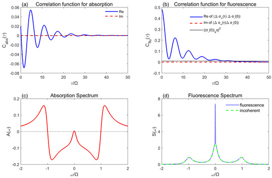
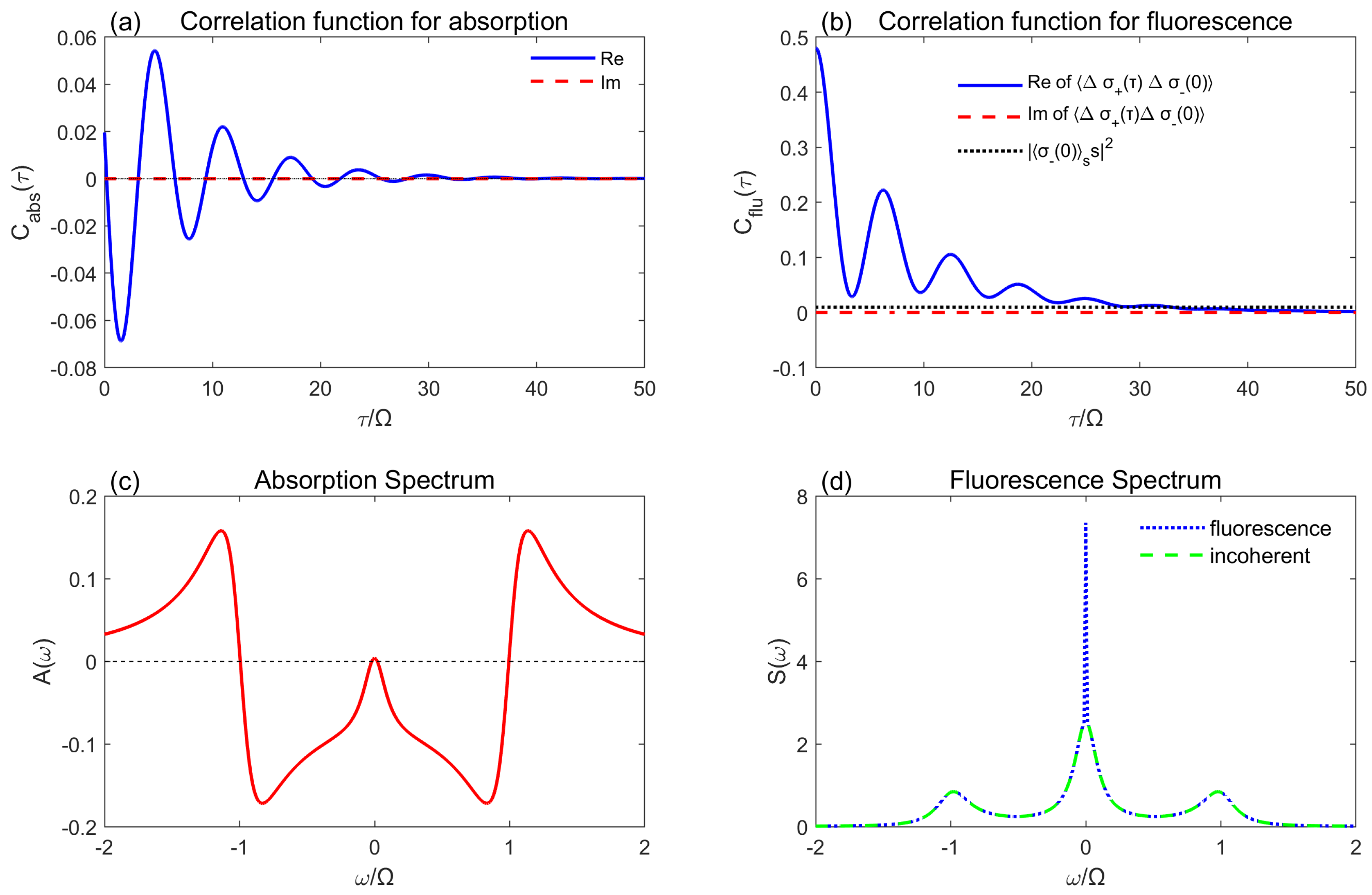
Figure 1 displays the steady-state spectral characteristics of a two-level system under strong laser driving ($\Omega =1$) with spontaneous emission ($\gamma =0.2$). Panels (a) and (b) show the time-domain evolution of the absorption and fluorescence correlation functions, respectively. The absorption correlation function $C_{\mathrm{abs}}\left(\tau \right)=⟨[{\sigma }_{-}\left(\tau \right),{\sigma }_{+}\left(0\right)]⟩$ exhibits damped oscillations at the Rabi frequency $\Omega$, reflecting the linear response of the dressed-state system to a weak probe field [43]. The fluorescence correlation function $C_{\mathrm{flu}}\left(\tau \right)=⟨{\sigma }_{+}\left(\tau \right){\sigma }_{-}\left(0\right)⟩-{\left|{⟨{\sigma }_{-}⟩}_{\mathrm{ss}}\right|}^2$ contains an oscillatory component from inelastic scattering and a constant background (black dashed line) from the subtracted elastic (coherent) component [1]. In the corresponding frequency-domain spectra [panels (c) and (d)], the absorption spectrum $A\left(\omega \right)$ exhibits a pronounced negative value at $\omega =0$–this is the Mollow gain region [43]: quantum interference among the dressed-state transition channels allows stimulated emission to dominate over absorption, enabling amplification of the probe field without population inversion. The sidebands are located at $\omega \approx \pm \Omega$; with $\Omega /\gamma =5$, the three resonances are fully resolved. The fluorescence spectrum $S\left(\omega \right)$ displays the canonical Mollow triplet structure [1], where the incoherent component (green dashed line), obtained after removing the central elastic $\delta$-peak, exhibits the characteristic three-peak lineshape [32,41].

Figure 1. Fluorescence and absorption spectra of a two-level system. (a) Correlation function for the absorption spectrum, (b) correlation function for the fluorescence spectrum, (c) absorption spectrum, and (d) fluorescence spectrum. The Rabi frequency $\Omega =1$ and the spontaneous emission rate $\gamma =0.2$ ($\Omega /\gamma =5$, strong driving regime) are adopted.

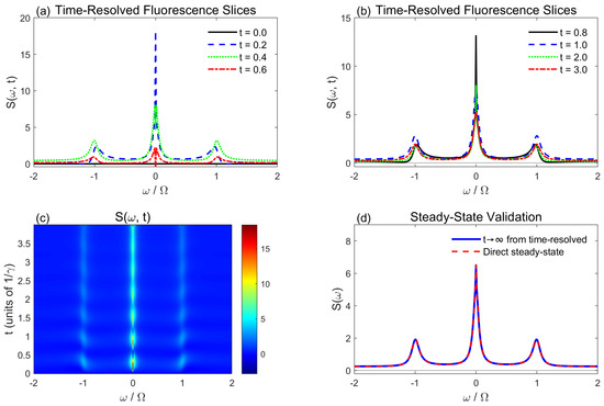
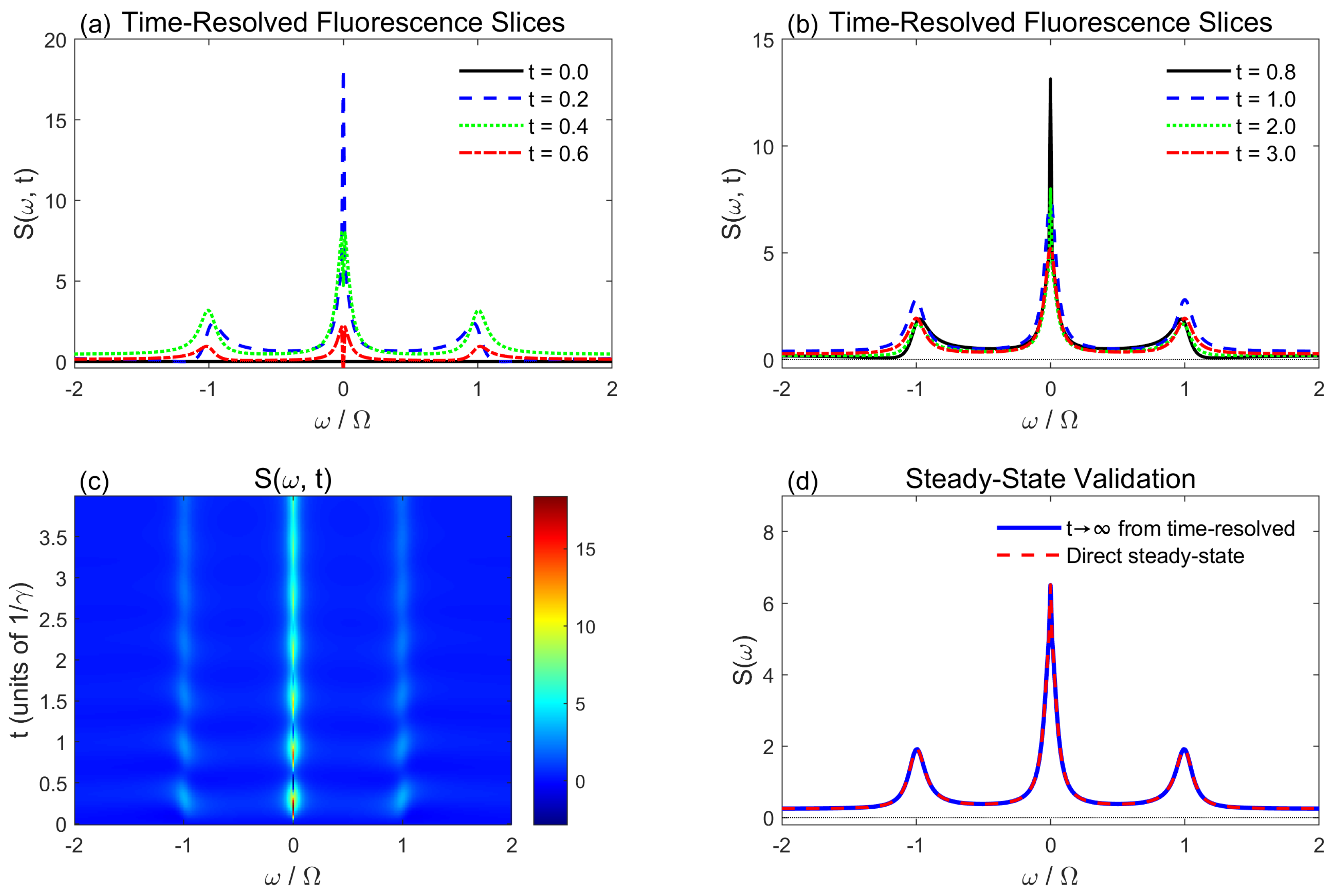
Figure 2 presents the complete dynamical build-up of the time-resolved fluorescence spectrum $S(\omega ,t)$, from the initial transient to steady-state establishment, for a system initially prepared in the ground state $\rho \left(0\right)=|g⟩⟨g|$ ($\Omega =1,\gamma =0.1$, giving $\Omega /\gamma =10$ for larger sideband splitting). Panels (a) and (b) show time slices at different evolution stages: at the initial moment ($t=0$), the atom is in the ground state and no signal is present; shortly thereafter, the fluorescence is almost entirely concentrated in the coherent scattering peak at $\omega =0$, while the inelastic sidebands are barely visible. As time progresses, the sideband intensities grow, accompanied by oscillations at the Rabi frequency $\Omega$, and the relative weight of the central coherent peak gradually decreases. By $t\gtrsim 3/\gamma$, the system has reached steady state and the lineshape no longer evolves. This process directly visualizes the transient establishment of dressed-state populations: population injected by the coherent drive is redistributed among the dressed states via spontaneous emission dissipation, and the sidebands—corresponding to transitions between dressed states—build up on a timescale set by the effective relaxation rate $\sim {\gamma }^{-1}$. Panel (c) presents a two-dimensional pseudocolor spectrogram of the full time-frequency evolution, clearly showing the persistent central peak and the gradual saturation of the sidebands over several ${\gamma }^{-1}$ time units. Panel (d) validates the self-consistency of the time-resolved method: the steady-state spectrum obtained by extrapolating the time evolution to $t\to \infty$ (blue solid line) coincides exactly with the steady-state solution from direct Lindblad master equation diagonalization (red dashed line), confirming that the system ultimately converges to the conventional Mollow triplet [1,7,44].

Figure 2. Time-resolved fluorescence of a two-level system for (a) early time slices at t = $0,0.2,0.4,0.6$, (b) later time slices at t = $0.8,1.0,2.0,3.0$, (c) full temporal evolution over the range [$0,4$], and (d) the long-time limit $t\to \infty$. The unit of time t is $1/\gamma$. Parameters $\Omega =1$ and $\gamma =0.2$ are used.

2.2. Time-Resolved Fluorescence of a Two-Level Atom with Bosonic Bath

To provide a more robust description, we employ the Dirac–Frenkel time-dependent variational principle combined with the multiple Davydov D₂ ansatz. This non-perturbative method allows us to treat the full system–bath Hamiltonian without neglecting counter-rotating terms or memory effects.

2.2.1. Two-Level System Coupled with Bosonic Bath

We consider a driven TLS coupled to a bosonic environment consisting of N harmonic oscillators. The total Hamiltonian is expressed as $\widehat{H}={\widehat{H}}_S+{\widehat{H}}_B+{\widehat{H}}_{SB}$. The system part, including the coherent drive, is given by

$${\widehat{H}}_S={\displaystyle \frac{\hslash {\omega }_0}{2}}{\sigma }_z+\hslash \Omega cos\left({\omega }_{L}t\right){\sigma }_x$$

(11)

where ${\omega }_0$ is the transition frequency, and $\Omega$ and ${\omega }_L$ denote the amplitude and frequency of the external drive, respectively. The environment and its interaction with the TLS are described by

$$\begin{array}{cc}\hfill {\widehat{H}}_B& ={\displaystyle \sum _{q=1}^N}\hslash {\omega }_q{\widehat{b}}_q^{†}{\widehat{b}}_q\hfill \end{array}$$

(12)

$$\begin{array}{cc}\hfill {\widehat{H}}_{SB}& ={\displaystyle \sum _{q=1}^N}{\displaystyle \frac{{\gamma }_q}{2}}\left(cos{\theta }_q{\sigma }_z+sin{\theta }_q{\sigma }_x\right)\left({\widehat{b}}_q^{†}+{\widehat{b}}_q\right)\hfill \end{array}$$

(13)

Here, ${\gamma }_q$ represents the coupling strength to the q-th mode, and ${\theta }_q$ is the mixing angle that determines the nature of the interaction: ${\theta }_q=\pi /2$ corresponds to pure dissipative (${\sigma }_x$) coupling, while ${\theta }_q=0$ represents pure dephasing (${\sigma }_z$) coupling. The mode-dependent coupling constants ${\gamma }_q$ are determined from the spectral density $J\left(\omega \right)$ via the standard discretization relation $J\left(\omega \right)={\sum }_{q=1}^N{\gamma }_q^2\delta (\omega -{\omega }_q),$ which, in the continuous limit, yields ${\gamma }_q=\sqrt{J\left({\omega }_q\right)\Delta {\omega }_q}$, where $\Delta {\omega }_q$ is the frequency spacing between adjacent modes. In practice, the bath frequency range $[0,{\omega }_c]$ is partitioned into $N_b$ intervals, and the coupling to the q-th mode is obtained as ${\gamma }_q^2={\int }_{{\omega }_q}^{{\omega }_q+\Delta {\omega }_q}J\left(\omega \right)d\omega .$ The bath’s influence is encapsulated in the spectral density $J\left(\omega \right)=2\alpha {\omega }_c^{1-s}{\omega }^s\Theta ({\omega }_c-\omega )$, where $\alpha$ is the bath’s coupling strength, ${\omega }_c$ is the high-frequency cutoff, and s defines the bath type: $s<1$ (sub-Ohmic), $s=1$ (Ohmic), $s>1$ (super-Ohmic). For the three spectral densities considered, this gives the scaling ${\gamma }_q\propto {\omega }_q^{s/2}$, so that the coupling per mode is largest at low frequencies for sub-Ohmic baths and shifted toward higher frequencies for super-Ohmic baths. A total of $N_b=150$ modes with linear discretization is employed, which ensures convergence for all cases studied.

We briefly comment on the discretization of the continuous spectral density and its connection to physical implementations. This linear discretization is physically motivated by circuit-QED platforms [16], where transmission-line resonators exhibit approximately uniform mode spacing at low frequencies. In such platforms, Ohmic spectral densities ($s=1$) arise from the frequency-independent impedance of a microwave transmission line coupled to a superconducting qubit [27,45], while sub-Ohmic densities ($s<1$) are engineered using hybrid metamaterial transmission lines with tailored dispersion [29], and super-Ohmic densities ($s>1$) describe the flux-noise environment probed in phase and flux qubits [46,47].

2.2.2. The Multi-D₂ State

To capture the non-trivial correlations between the TLS and the bath, we adopt the multi-D₂ ansatz with multiplicity M:

$$\left|D_2^M\left(t\right)\right.⟩={\displaystyle \sum _{i=1}^M}\left[A_i\left(t\right)|\uparrow ⟩+B_i\left(t\right)|\downarrow ⟩\right]\otimes exp\left[{\displaystyle \sum _{q=1}^N}\left(f_{iq}\left(t\right){\widehat{b}}_q^{†}-\mathrm{c}.\mathrm{c}.\right)\right]|0⟩$$

(14)

where $A_i\left(t\right)$, $B_i\left(t\right)$ are the complex probability amplitudes for the TLS states, and $f_{iq}\left(t\right)$ are the time-dependent displacements of the bath modes.

The evolution of these $M(2+N)$ parameters is governed by the Euler–Lagrange equations derived from the Lagrangian $L=\left.⟨D_2^M\right|{\displaystyle \frac{i\hslash }{2}}{\overleftrightarrow{\partial }}_t-\widehat{H}\left|D_2^M\right.⟩$. This variational approach provides a numerically efficient way to track the many-body dynamics by projecting the Schrödinger equation onto a restricted but physically motivated manifold of coherent states.

By numerically integrating the equations of motion, we track the temporal evolution of the variational parameters $A_i\left(t\right)$, $B_i\left(t\right)$, and $f_{iq}\left(t\right)$, which allows for the direct evaluation of various physical observables.

The population inversion of the TLS, denoted by $P_z\left(t\right)$, is determined by

$$\begin{array}{cc}\hfill P_z\left(t\right)& =⟨D_2^M\left(t\right)\left|{\sigma }_z\right|D_2^M\left(t\right)⟩\hfill \\ \hfill & ={\displaystyle \sum _{i,j=1}^M}\left(A_j^{*}{A}_i-B_j^{*}{B}_i\right)S_{ji},\hfill \end{array}$$

(15)

where $S_{ji}$ represents the Debye–Waller factor (overlap of the bosonic coherent states).

A significant advantage of the Multi-$D_2$ approach is its ability to explicitly resolve the state of the environment. Specifically, the photon occupation in the q-th bath mode at time t is given by

$$\begin{array}{cc}\hfill S({\omega }_q,t)& =⟨D_2^M\left(t\right)\left|b_q^{†}{b}_q\right|D_2^M\left(t\right)⟩\hfill \\ \hfill & ={\displaystyle \sum _{i,j=1}^M}\left(A_j^{*}{A}_i+B_j^{*}{B}_i\right)f_{jq}^{*}{S}_{ji}{f}_{iq}.\hfill \end{array}$$

(16)

From a physical perspective, $S({\omega }_q,t)$ quantifies the number of photons scattered into the reservoir modes, which are initially in the vacuum state. Consequently, the distribution $S({\omega }_q,t)$ as a function of frequency ${\omega }_q$ and time t serves as a direct representation of the time-resolved fluorescence spectrum. Unlike master-equation techniques that trace out the reservoir degrees of freedom, our method retains the full information of the bath, allowing the transient spectrum to naturally evolve toward its steady-state limit, ${lim}_{t\to \infty }S({\omega }_q,t)=S\left({\omega }_q\right)$.

2.2.3. Benchmark: Off-Diagonal Coupling with an Ohmic Bath

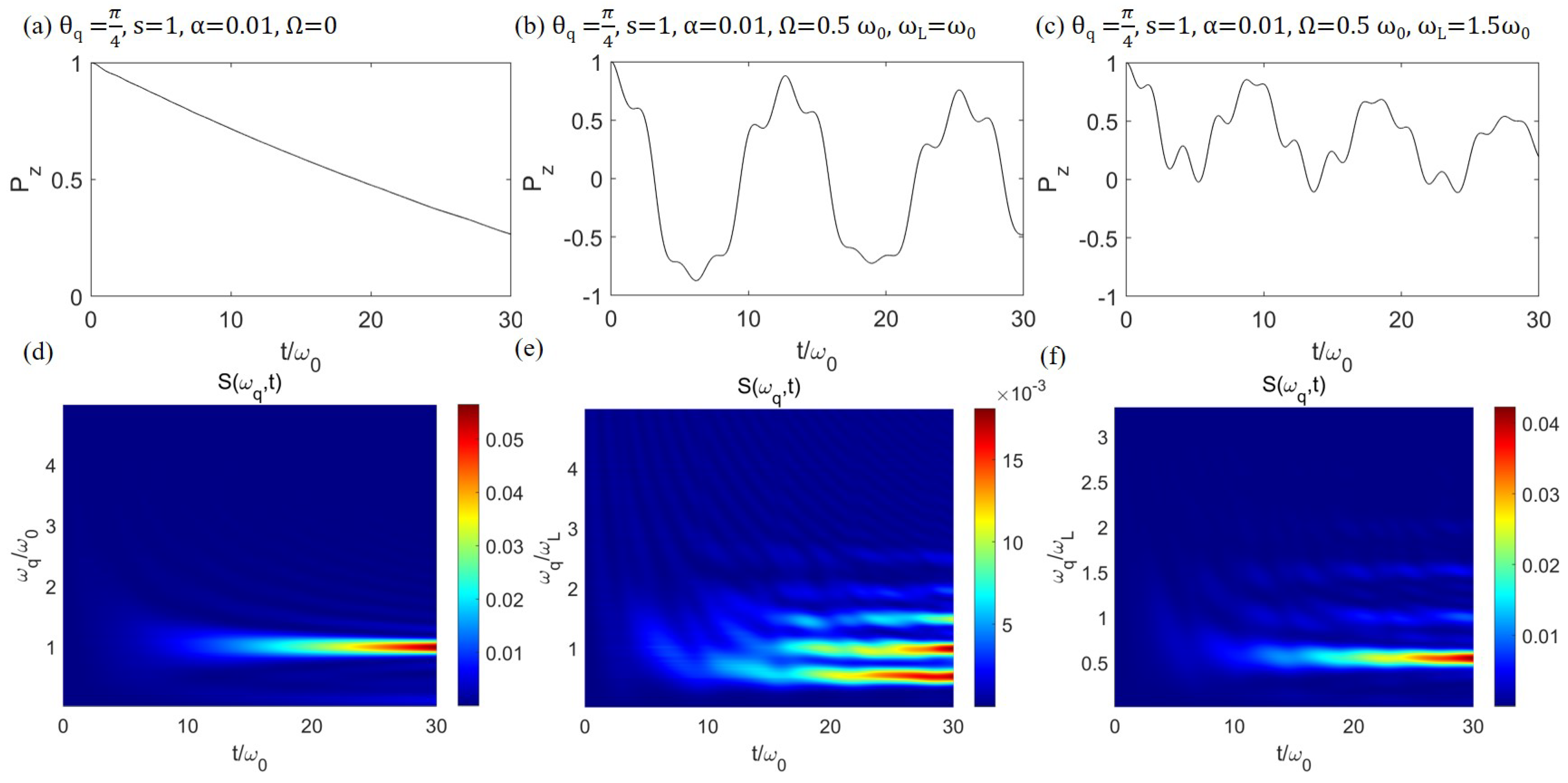
We first benchmark the multi-D₂ approach by considering the case of pure off-diagonal coupling (${\theta }_q=\pi /2$, i.e., ${\sigma }_x$ coupling) with an Ohmic spectral density ($s=1$), which corresponds to the system studied in Ref. [25] using the multi-D₁ ansatz. This choice is motivated by two considerations. First, the ${\sigma }_x$-coupled spin-boson model with an Ohmic bath is the most extensively characterized configuration in the literature: the HEOM and multi-D₁ results of Ref. [25] have been cross-validated against each other, providing a stringent benchmark for any new method. Second, this case establishes a direct comparison point for the ${\sigma }_x$-coupling results presented in Section 2.2.4 and Section 2.2.5, allowing the effects of the spectral density exponent s to be assessed relative to this well-characterized Ohmic baseline. The parameters are chosen to match those of Ref. [25]: coupling strength $\alpha =0.01$, cutoff frequency ${\omega }_c=5{\omega }_0$, and $N_b=150$ bath modes. Notably, for the multi-D₂ ansatz, a multiplicity of M = 4 is sufficient to achieve excellent agreement with the HEOM benchmark across all driving conditions considered, whereas the multi-D₁ ansatz in Ref. [25] requires M = 8 for comparable convergence. This improved efficiency arises from the ${\sigma }_z$-basis formulation in this work, which provides a more natural parametrization of the system–bath entanglement for the present Hamiltonian.

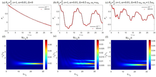
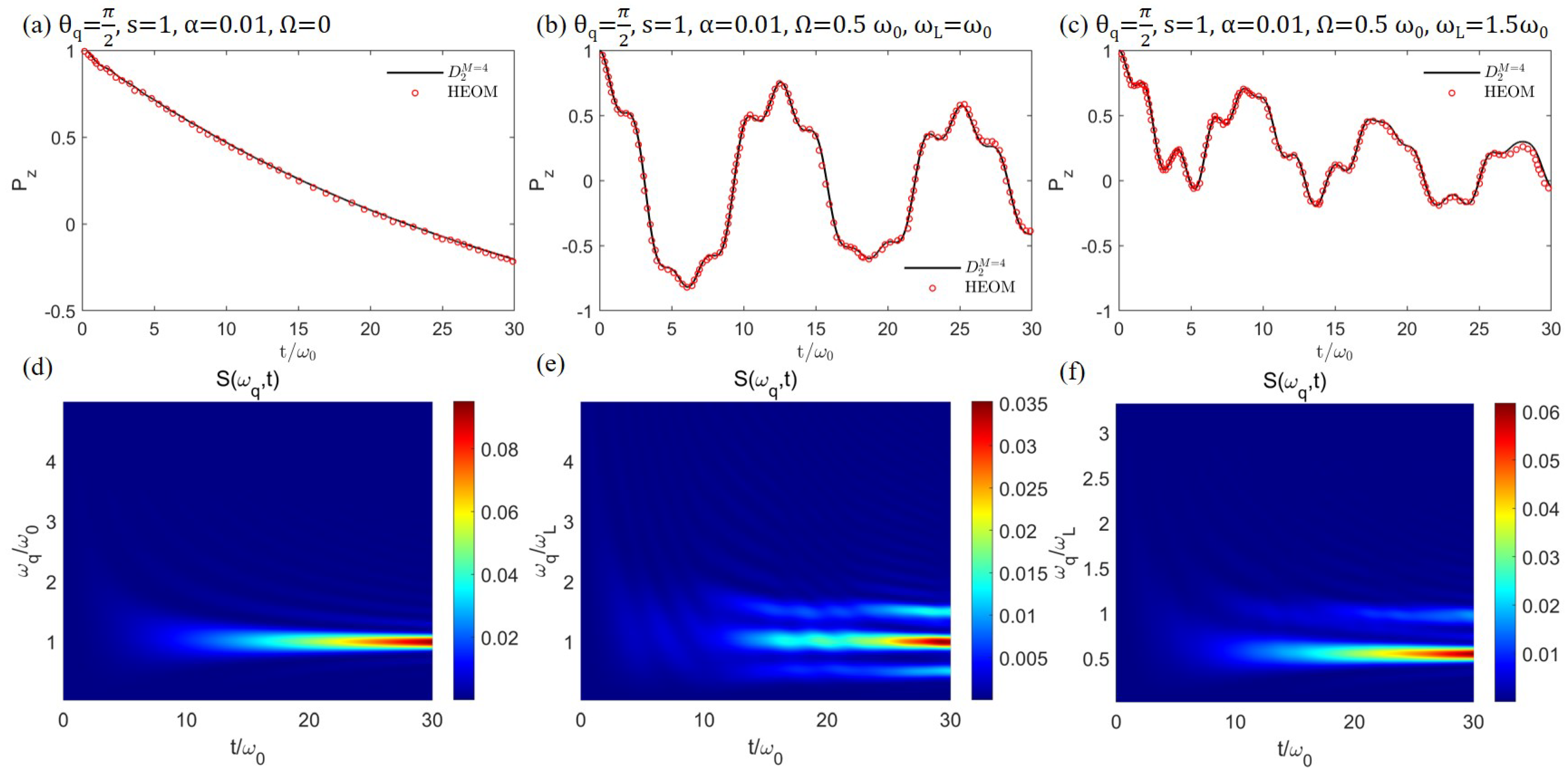
Figure 3 presents the dynamics for three driving conditions: (a) $\Omega =0$ (spontaneous decay), (b) $\Omega =0.5{\omega }_0$ with resonant driving ${\omega }_L={\omega }_0$, and (c) $\Omega =0.5{\omega }_0$ with off-resonant driving ${\omega }_L=1.5{\omega }_0$. Panels (a)–(c) show the population difference $P_z\left(t\right)=⟨{\sigma }_z⟩$, while panels (d)–(f) display the corresponding time-resolved fluorescence spectra $S(\omega ,t)$.

Figure 3. Dynamics of the population difference between the ground and excited states for off-diagonal qubit–bath coupling with ${\theta }_q={\displaystyle \frac{\pi }{2}}$, Ohmic spectral density of s = 1, qubit–bath coupling strength of $\alpha$ = 0.01, and (a) $\Omega$ = 0, (b) $\Omega$ = 0.5${\omega }_0$ and ${\omega }_L$ = ${\omega }_0$, and (c) $\Omega$ = 0.5${\omega }_0$ and ${\omega }_L$ = 1.5${\omega }_0$. (d–f) Time-resolved fluorescence spectra of aforementioned cases (a–c), respectively.

For the undriven case [Figure 3a], the TLS initially prepared in the excited state undergoes spontaneous decay to the ground state. The multi-D₂ result for $P_z\left(t\right)$ is in excellent agreement with the HEOM benchmark and the multi-D₁ result of Ref. [25], confirming the accuracy of the variational approach. The corresponding time-resolved spectrum [Figure 3d] shows a single emission peak at $\omega ={\omega }_0$ that emerges monotonically in time, corresponding to the spontaneous emission of a photon at the TLS transition frequency.

Under resonant strong driving [Figure 3b], the population exhibits damped Rabi oscillations at the generalized Rabi frequency ${\Omega }_R=\sqrt{{\Omega }^2+{({\omega }_L-{\omega }_0)}^2}=\Omega$. The $P_z\left(t\right)$ trace from multi-D₂ coincides perfectly with that from HEOM, validating the consistency between the two ansätze for the reduced qubit dynamics. The time-resolved fluorescence spectrum [Figure 3e] reveals the dynamical build-up of the Mollow triplet: at early times, the spectrum is dominated by the coherent elastic peak at the driving frequency; as time progresses, the two inelastic sidebands emerge at $\omega \approx {\omega }_0\pm \Omega$, and the system eventually reaches a steady-state Mollow triplet structure. The spectral asymmetry observed at intermediate times is consistent with the turn-on dynamics reported in Ref. [25], arising from the frequency-dependent coupling strength between TLS and individual bath modes.

For off-resonant driving [Figure 3c], the Rabi oscillations occur at the generalized Rabi frequency ${\Omega }_R=\sqrt{{\Omega }^2+{({\omega }_L-{\omega }_0)}^2}>\Omega$, and the steady-state population saturates at a value determined by the detuning. The corresponding time-resolved spectrum [Figure 3f] shows a broader spectral distribution with the sidebands shifted according to ${\Omega }_R$, consistent with the predictions of the dressed-state picture.

We note that the photon number $S({\omega }_q,t)$ from multi-D₂ captures the correct qualitative spectral features—peak positions, relative intensities, and temporal evolution. The present multi-D₂ framework, formulated in the ${\sigma }_z$ basis, converges with fewer multiplicities (M = 4 vs. M = 8 for multi-D₁) and, crucially, accommodates arbitrary coupling types beyond the pure ${\sigma }_x$ case, which we exploit in the following sections.

2.2.4. Effect of Spectral Density: Sub-Ohmic and Super-Ohmic Reservoirs at at Fixed $\alpha$ and Fixed $J\left({\omega }_0\right)$

Fixed $\alpha$: Shape Effects at Constant Coupling Strength

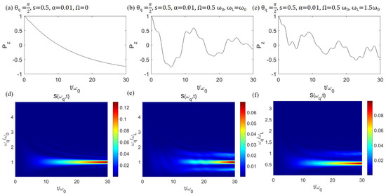
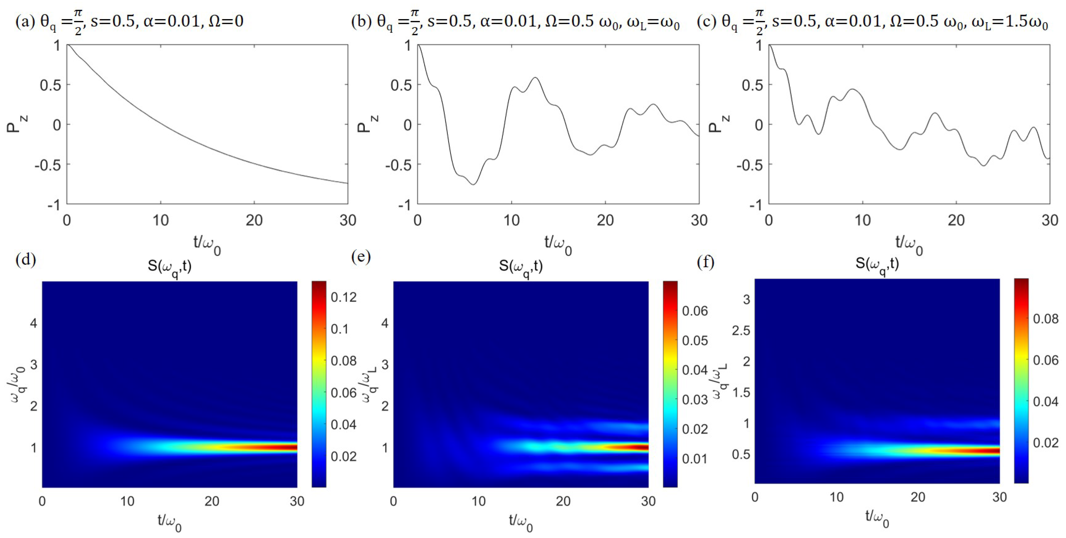
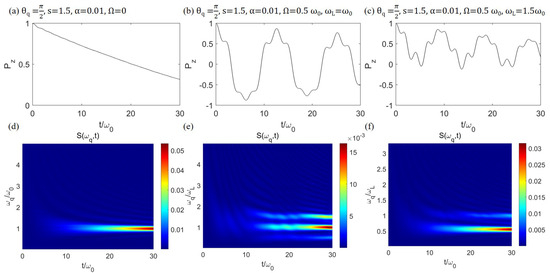
Having validated the multi-D₂ approach for the Ohmic case, we now investigate how the spectral density exponent s modifies the time-resolved fluorescence spectrum. Figure 4 shows the results for a sub-Ohmic bath ($s=0.5$, ${\theta }_q=\pi /2$, $\alpha =0.01$), while Figure 5 presents the super-Ohmic case ($s=1.5$, ${\theta }_q=\pi /2$, $\alpha =0.01$). In all cases, the same driving conditions as in Figure 3 are used for direct comparison.

Figure 4. Dynamics of the population difference between the ground and excited states for off-diagonal qubit–bath coupling with ${\theta }_q={\displaystyle \frac{\pi }{2}}$, sub-Ohmic spectral density of s = 0.5, qubit–bath coupling strength of $\alpha$ = 0.01, and (a) $\Omega$ = 0, (b) $\Omega$ = 0.5${\omega }_0$ and ${\omega }_L$ = ${\omega }_0$, and (c) $\Omega$ = 0.5${\omega }_0$ and ${\omega }_L$ = 1.5${\omega }_0$. (d–f) Time-resolved fluorescence spectra of aforementioned cases (a–c), respectively.

Figure 5. Dynamics of the population difference between the ground and excited states for off-diagonal qubit–bath coupling with ${\theta }_q={\displaystyle \frac{\pi }{2}}$, super-Ohmic spectral density of s = 1.5, qubit–bath coupling strength of $\alpha$ = 0.01, and (a) $\Omega$ = 0, (b) $\Omega$ = 0.5${\omega }_0$ and ${\omega }_L$ = ${\omega }_0$, and (c) $\Omega$ = 0.5${\omega }_0$ and ${\omega }_L$ = 1.5${\omega }_0$. (d–f) Time-resolved fluorescence spectra of aforementioned cases (a–c), respectively.

For the sub-Ohmic case (Figure 4), the spectral density $J\left(\omega \right)\propto {\omega }^{0.5}$ at low frequencies provides a larger spectral weight near the system transition frequency ${\omega }_0$ (since ${\omega }_0<{\omega }_c$), leading to more efficient resonant energy relaxation. This enhanced effective coupling manifests clearly in the population dynamics. In the undriven case [Figure 4a], the spontaneous decay of $P_z$ proceeds faster than its Ohmic counterpart. Under resonant driving [Figure 4b], the Rabi oscillations exhibit more rapid damping, reflecting the stronger dissipation arising from the abundant low-frequency bath modes. Correspondingly, the time-resolved fluorescence spectra [Figure 4d–f] display higher overall intensity compared to the Ohmic case, indicating enhanced photon scattering into the bath. Notably, in Figure 4e, the Mollow triplet shows improved symmetry restoration, suggesting that the faster dissipative dynamics facilitate a more rapid approach toward the symmetric steady-state configuration of the dressed-state manifold.

For the super-Ohmic case (Figure 5), the spectral density $J\left(\omega \right)\propto {\omega }^{1.5}$ suppresses low-frequency modes while enhancing high-frequency modes relative to the Ohmic distribution. Since the system dynamics is predominantly governed by bath modes resonant with the transition frequency ${\omega }_0$, the suppression of these resonant modes reduces the effective qubit-bath coupling strength. This leads to qualitatively different dynamics. In the undriven case [Figure 5a], the spontaneous decay of $P_z$ proceeds the most slowly among the three spectral densities, and the system has not reached its steady state within the computed time window. Under resonant driving [Figure 5b], the Rabi oscillations exhibit the weakest damping, and oscillatory features persist well beyond the time scales where the Ohmic and sub-Ohmic counterparts have already damped out. The time-resolved spectra [Figure 5d–f] show the weakest fluorescence intensity among the three cases, consistent with the reduced effective dissipation rate that suppresses photon emission into the bath.

A systematic comparison across the three spectral densities reveals that the effective dissipation rate follows a distinct ordering: the sub-Ohmic bath ($s=0.5$) induces the fastest relaxation and strongest fluorescence, followed by the Ohmic bath ($s=1$), while the super-Ohmic bath ($s=1.5$) yields the slowest dynamics and weakest fluorescence within our observation window. This behavior can be understood from the spectral density evaluated at the system transition frequency: $J\left({\omega }_0\right)\propto {\omega }_0^s$. For ${\omega }_0<{\omega }_c$ (the present case with ${\omega }_c=5{\omega }_0$), the sub-Ohmic distribution provides the largest spectral weight at resonance, while the super-Ohmic distribution provides the smallest—opposite to the trend of the total integrated coupling strength ${\int }_0^{{\omega }_c}J\left(\omega \right)d\omega =2\alpha {\omega }_c^2/(s+1)$, which increases with s. This indicates that the fluorescence dynamics is primarily governed by the resonant component of the spectral density rather than the total integrated coupling, highlighting that the spectral density exponent provides an effective control parameter for engineering transient fluorescence properties: sub-Ohmic reservoirs enhance both the relaxation rate and fluorescence output, while super-Ohmic reservoirs prolong the transient regime and suppress dissipative emission.

While this analysis establishes the dominant role of the resonant spectral weight under fixed coupling strength $\alpha$, it leaves open the question of whether the observed differences between sub-Ohmic and Ohmic baths persist when $J\left({\omega }_0\right)$ itself is held constant, and whether the super-Ohmic suppression is robust against such a rescaling. We address this in the following subsection.

Fixed $J\left({\omega }_0\right)$: Disentangling Resonant Weight from Spectral Shape

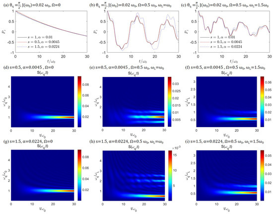
To disentangle the resonant-coupling effect from the genuine spectral-shape effect, we fix the resonant spectral weight at $J\left({\omega }_0\right)=0.02{\omega }_0$ and adjust $\alpha$ accordingly: $\alpha =0.0045$ for $s=0.5$, $\alpha =0.01$ for $s=1$, and $\alpha =0.0224$ for $s=1.5$. Figure 6 presents the resulting dynamics for the same driving conditions as in Figure 3.

Figure 6. Dynamics under fixed resonant spectral weight $J\left({\omega }_0\right)=0.02{\omega }_0$ for off-diagonal qubit–bath coupling (${\theta }_q=\pi /2$). (a–c): Population difference $P_z\left(t\right)$ for $s=1$ ($\alpha =0.01$, black solid), $s=0.5$ ($\alpha =0.0045$, red dash-dotted), and $s=1.5$ ($\alpha =0.0224$, blue dashed), in the undriven (a), resonantly driven (b), and off-resonantly driven (c) cases. (d–f): Time-resolved fluorescence spectra for the sub-Ohmic case ($s=0.5$); (g–i): for the super-Ohmic case ($s=1.5$).

In the undriven case [Figure 6a], the population dynamics for all three spectral densities collapse onto a single curve, and the fluorescence spectra [Figure 6d,g and Figure 3d] exhibit comparable intensities. This indicates that spontaneous decay is governed almost exclusively by $J\left({\omega }_0\right)$, with the spectral shape playing a negligible role when the system only probes the resonant frequency ${\omega }_0$.

Under resonant driving [Figure 6b], the sub-Ohmic ($s=0.5$, red dash-dotted) and Ohmic ($s=1$, black solid) curves lie much closer to each other than in the fixed-$\alpha$ comparison of Figure 3b, confirming that the faster relaxation previously seen for $s=0.5$ was largely due to its larger $J\left({\omega }_0\right)$. Nevertheless, residual differences persist: the sub-Ohmic case shows slightly faster damping and an enhanced low-frequency emission tail in the time-resolved spectrum [Figure 6e], which is absent in the Ohmic benchmark [Figure 3d]. This low-frequency enhancement originates from the larger density of low-frequency bath modes in the sub-Ohmic distribution; these modes, although off-resonant with the bare transition ${\omega }_0$, couple to the dressed states formed under strong driving and facilitate inter-dressed-state relaxation, thereby accelerating the restoration of the symmetric Mollow-triplet steady state.

Most notably, under resonant driving, the super-Ohmic case ($s=1.5$, blue dashed) exhibits a dramatically weaker fluorescence intensity [Figure 6h] compared with both its Ohmic [Figure 3e] and sub-Ohmic [Figure 6e] counterparts. Because the lower Mollow sideband lies at ${\omega }_q\approx {\omega }_0-\Omega =0.5{\omega }_0$, it falls into the frequency region where the super-Ohmic spectral density is strongly depleted. The bath therefore cannot efficiently accept energy from the sideband transitions, leading to suppressed sideband emission and slower dressed-state relaxation despite identical $J\left({\omega }_0\right)$. Under off-resonant driving [Figure 6c,f,i and Figure 3f], by contrast, the differences between all three spectral densities are substantially smaller, indicating that the super-Ohmic shape effect is most pronounced when the driven system probes the suppressed low-frequency region of the bath.

2.2.5. Pure Dephasing: Diagonal (${\sigma }_z$) Coupling

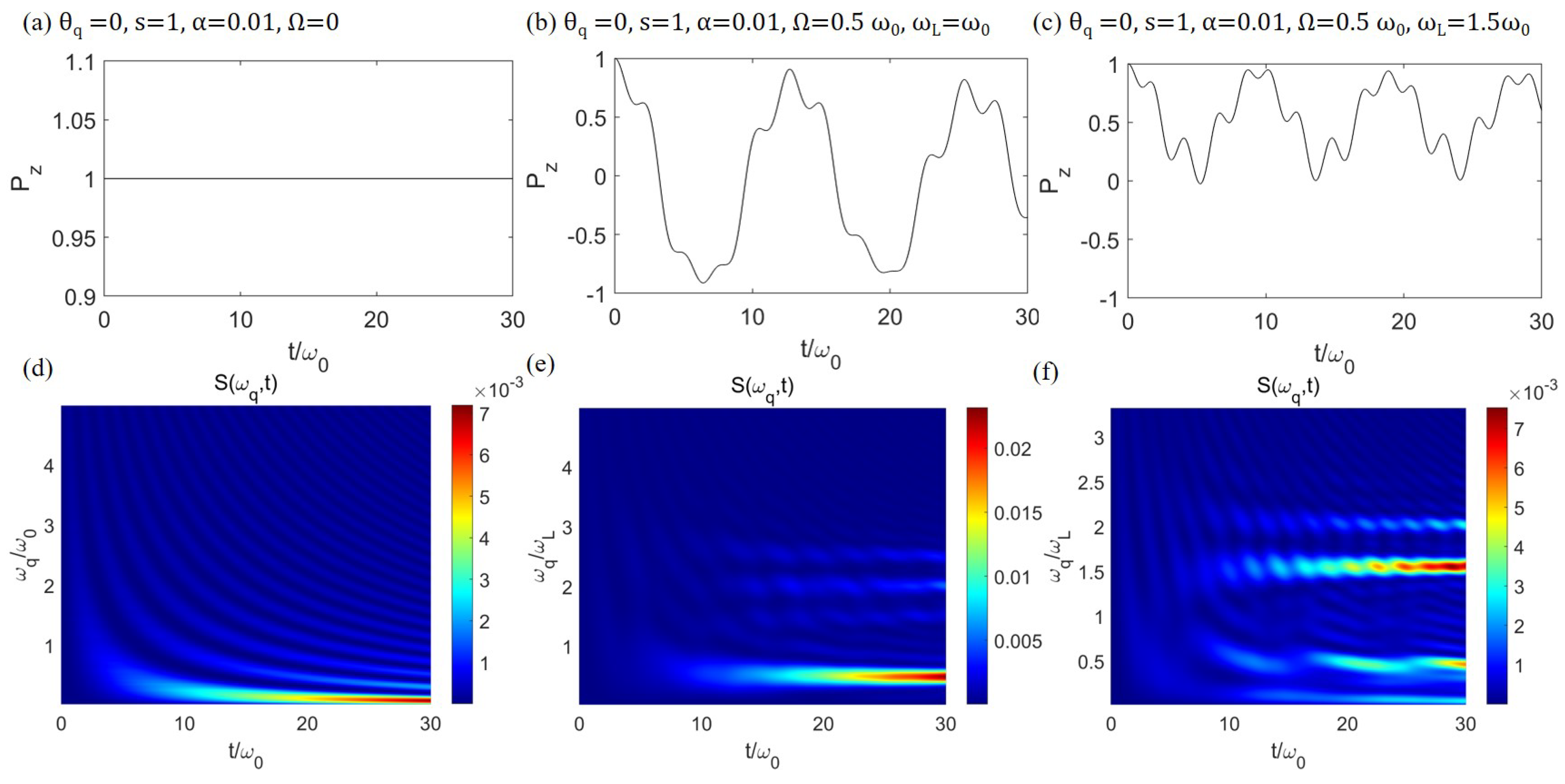
We now turn to the case of pure diagonal coupling (${\theta }_q=0$, i.e., ${\sigma }_z$ coupling) with an Ohmic spectral density ($s=1$, $\alpha =0.01$), as shown in Figure 7. This coupling type corresponds to pure dephasing, where the bath modulates the transition frequency of the TLS without directly inducing transitions between the bare energy levels.

Figure 7. Dynamics of the population difference between the ground and excited states for diagonal qubit–bath coupling with ${\theta }_q=0$, Ohmic spectral density of s = 1, qubit–bath coupling strength of $\alpha$ = 0.01, and (a) $\Omega$ = 0, (b) $\Omega$ = 0.5${\omega }_0$ and ${\omega }_L$ = ${\omega }_0$, and (c) $\Omega$ = 0.5${\omega }_0$ and ${\omega }_L$ = 1.5${\omega }_0$. (d–f) Time-resolved fluorescence spectra of aforementioned cases (a–c), respectively.

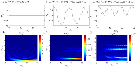
The population dynamics $P_z\left(t\right)$ [Figure 7a–c] exhibits a striking difference from the off-diagonal case. For all three driving conditions, $P_z\left(t\right)$ shows no decay—the Rabi oscillations persist indefinitely without damping. This is a direct consequence of the ${\sigma }_z$ coupling: since the bath operator commutes with the bare TLS Hamiltonian, it does not cause population relaxation ($t\to \infty$).

However, the time-resolved fluorescence spectrum $S({\omega }_q,t)$ reveals that the radiative properties are not entirely suppressed. The interplay between the coherent drive and the ${\sigma }_z$ coupling enables a specific radiative process. In the resonant case [Figure 7e, ${\omega }_L={\omega }_0$], a distinct emission peak is observed at ${\omega }_q/{\omega }_L\approx 0.5$. Given that the driving strength is set to $\Omega =0.5{\omega }_0$, this peak corresponds exactly to the Rabi frequency $\Omega$ (which equals the generalized Rabi frequency ${\Omega }_R$ when the detuning $\Delta =0$).

This phenomenon can be understood through the dressed-state picture: the resonant drive hybridizes the TLS levels into dressed states separated by energy $\hslash \Omega$. In this dressed basis, the ${\sigma }_z$ operator acquires purely off-diagonal components, thereby inducing transitions between the dressed states and exciting the bath modes at the frequency $\Omega$. This represents a direct observation of dressed-state transitions mediated by the dephasing channel, a feature that remains hidden in the population dynamics.

In the off-resonant case [Figure 7f, ${\omega }_L=1.5{\omega }_0$], the spectral signature shifts to ${\omega }_q/{\omega }_L=1.5$ (corresponding to ${\omega }_q=2.25{\omega }_0$). The appearance of this peak at a fractional multiple of the driving frequency suggests a more complex non-linear scattering process where the ${\sigma }_z$ coupling facilitates energy exchange at higher-order combinations of the driving and system frequencies. In contrast, the undriven case [Figure 7d] remains dark, as no dressed states are formed to facilitate radiation.

These results demonstrate that the time-resolved fluorescence spectrum $S({\omega }_q,t)$ is a powerful tool for revealing the underlying dressed-state structure of a driven TLS, even in environments dominated by pure dephasing where traditional measurements of $P_z\left(t\right)$ show no signs of relaxation.

2.2.6. Mixed Coupling

In realistic solid-state environments, a TLS is often simultaneously coupled to multiple decoherence channels. To investigate this interplay, we consider a mixed coupling scenario with ${\theta }_q={45}^{\circ }$ for all bath modes, where the system–bath interaction includes equal contributions from ${\sigma }_x$ and ${\sigma }_z$ operators. The results are presented in Figure 8.

Figure 8. Dynamics of the population difference between the ground and excited states for mixing qubit–bath coupling with ${\theta }_q={\displaystyle \frac{\pi }{4}}$, Ohmic spectral density of s = 1, qubit–bath coupling strength of $\alpha$ = 0.01, and (a) $\Omega$ = 0, (b) $\Omega$ = 0.5${\omega }_0$ and ${\omega }_L$ = ${\omega }_0$, and (c) $\Omega$ = 0.5${\omega }_0$ and ${\omega }_L$ = 1.5${\omega }_0$. (d–f) Time-resolved fluorescence spectra of aforementioned cases (a–c), respectively.

The population dynamics $P_z\left(t\right)$ [Figure 8a–c] shows that the Rabi oscillations persist for a longer duration compared to the pure ${\sigma }_x$ case (Figure 3). This slower decay of $P_z\left(t\right)$ is attributed to the reduced effective coupling to the dissipative ${\sigma }_x$ channel; since the total coupling strength is now shared between ${\sigma }_x$ and ${\sigma }_z$, the population relaxation rate ($1/T_1$) decreases, leading to more sustained oscillations.

The time-resolved fluorescence spectrum $S({\omega }_q,t)$ [Figure 8d–f] reveals a complex superposition of radiative signatures. In the resonant driving case [Figure 8e], the Mollow triplet structure is clearly identifiable, yet the relative intensities of the peaks are significantly altered. Most notably, the emission peak at ${\omega }_q/{\omega }_L\approx 0.5$ (corresponding to the Rabi frequency $\Omega$) emerges as the most prominent feature, even though the overall fluorescence intensity is relatively weak.

This dominance of the $\Omega$-frequency peak confirms that the ${\sigma }_z$-induced radiative mechanism—discussed in Section 2.2.5—remains highly efficient even in the presence of a dissipative ${\sigma }_x$ channel. The ${\sigma }_z$ component of the bath effectively “probes” the dressed-state splitting more strongly than the ${\sigma }_x$ component induces standard Mollow transitions.

In the off-resonant case [Figure 8f], the spectrum exhibits a multi-peak structure that combines the features of both coupling types, with the peak positions dictated by the interplay of the driving frequency and the generalized Rabi frequency. The ability of the multi-D₂ method to resolve these competing spectral features—where the strongest emission does not necessarily occur at the bare or driving frequencies—demonstrates its superior capability in simulating the dynamics of quantum emitters in complex, multi-channel environments.

2.2.7. Comparative Summary

Having examined the individual configurations, we summarize the key similarities and distinctions among Figure 4, Figure 5, Figure 6, Figure 7 and Figure 8 to distill the physical picture. Table 1 provides a concise overview.

Table 1. Summary of the time-resolved fluorescence characteristics for different coupling types and spectral densities.

Configuration	${\mathit{P}}_{\mathit{z}}\left(\mathit{t}\right)$ Behavior	Fluorescence Features	Dominant Mechanism
${\sigma }_x$, sub-Ohmic, fixed $\alpha$ (Figure 4)	Fastest damping	Strong Mollow triplet, fast symmetry restoration	Large $J\left({\omega }_0\right)$ plus abundant low-$\omega$ modes
${\sigma }_x$, Ohmic (Figure 3)	Damped Rabi oscillations	Mollow triplet	$T_1$ relaxation
${\sigma }_x$, super-Ohmic, fixed $\alpha$ (Figure 5)	Slowest damping	Weak Mollow triplet, persistent oscillations	Small $J\left({\omega }_0\right)$ suppresses resonant coupling
${\sigma }_x$, fixed $J\left({\omega }_0\right)$ (Figure 6)	Nearly identical for all s (undriven); sub-Ohmic ≈ Ohmic under driving	Super-Ohmic sideband strongly suppressed under resonant driving	$J\left({\omega }_0\right)$ governs $T_1$; shape matters via sideband frequencies
${\sigma }_z$, Ohmic (Figure 7)	No decay ($T_1\to \infty$)	Single peak at $\Omega$	Dephasing-mediated dressed-state transition
Mixed $\theta =\pi /4$, Ohmic (Figure 8)	Slow decay	Mollow triplet + dominant $\Omega$ peak	Competing $T_1$ and $T_2$ channels

Several general trends emerge from this comparison. First, Figure 4 and Figure 5, obtained with fixed $\alpha$, appear qualitatively similar: both exhibit the Mollow-triplet structure characteristic of ${\sigma }_x$ coupling, with the primary difference being the decay rate and overall intensity. The controlled comparison (Figure 6) reveals the origin of this difference: it stems predominantly from the resonant spectral weight $J\left({\omega }_0\right)$, which varies by a factor of five between $s=0.5$ and $s=1.5$ at fixed $\alpha$, rather than from the spectral density shape itself. Indeed, when $J\left({\omega }_0\right)$ is held constant, the undriven decay curves for all three s values collapse onto a single line [Figure 6a], and the driven sub-Ohmic and Ohmic dynamics become nearly indistinguishable [Figure 6b].

Second, a genuine shape effect survives the $J\left({\omega }_0\right)$ rescaling, and it is selective in frequency: under resonant driving, the super-Ohmic spectrum is dramatically weakened [Figure 6h] because the lower Mollow sideband at $\omega \approx {\omega }_0-\Omega =0.5{\omega }_0$ falls in the depleted low-frequency region of the super-Ohmic bath, whereas the off-resonant case [Figure 6i] shows only modest differences. Thus the spectral density exponent s does not merely rescale the overall dissipation rate; it redistributes the dissipation weight among the Mollow sidebands, an effect that is invisible in population dynamics alone and most pronounced when a sideband is tuned into a spectrally depleted region.

Third, Figure 7 and Figure 8 demonstrate that the fluorescence spectrum probes coupling channels that population measurements cannot resolve. Pure ${\sigma }_z$ coupling leaves $P_z\left(t\right)$ undamped, yet the spectrum displays a clear peak at the Rabi frequency $\Omega$ [Figure 7e], signaling dephasing-mediated dressed-state transitions. In the mixed case [Figure 8e], the ${\sigma }_z$-induced $\Omega$ peak dominates the spectrum even though the ${\sigma }_x$ channel is the sole source of population relaxation, showing that the fluorescence spectrum is more sensitive to the dephasing channel than population dynamics alone.

Taken together, these results establish two practical guidelines: (i) for a resonantly driven TLS, the effective dissipation rate is governed almost exclusively by the resonant spectral weight $J\left({\omega }_0\right)$, irrespective of the global spectral density shape; and (ii) the spectral density exponent s acts as a frequency-selective knob that modulates emission at the Mollow sidebands, providing an experimentally controllable handle—via engineered spectral densities (sub-Ohmic metamaterial lines [29], super-Ohmic flux-noise environments [46,47])—for shaping transient fluorescence.

3. Conclusions and Outlook

In this work, we systematically investigated the time-resolved fluorescence spectra of a driven two-level system using the multi-D₂ variational method in the ${\sigma }_z$ basis. Compared to the conventional multi-D₁ approach, the multi-D₂ ansatz offers faster convergence ($M=4$ suffices where $M=8$ was previously needed) and naturally accommodates both ${\sigma }_z$ coupling and mixed coupling configurations, which were difficult to treat within a unified framework. Our calculations reveal that under resonant driving, ${\sigma }_z$ coupling produces a fluorescence peak at ${\omega }_q/{\omega }_L\approx 0.5$, arising from dressed-state transitions mediated by longitudinal coupling. Mixed coupling simultaneously generates the Mollow triplet and the ${\sigma }_z$ peak, with $P_z$ decay slower than in the pure ${\sigma }_x$ case, highlighting the distinct roles of different coupling channels in relaxation dynamics. Furthermore, the spectral density exponent s is revealed to operate through two distinct mechanisms: (i) a dominant resonant-scaling effect via $J\left({\omega }_0\right)$ that governs the overall dissipation rate, and (ii) a secondary shape-dependent channel that modulates the low-frequency bath response. In the undriven limit, mechanism (i) fully accounts for the dynamics, as confirmed by the collapse of all three s values onto a single curve when $J\left({\omega }_0\right)$ is matched. Under resonant driving, mechanism (ii) becomes manifest: the sub-Ohmic bath retains a larger low-frequency mode density that facilitates dressed-state relaxation and restores Mollow-triplet symmetry more efficiently than the Ohmic bath, whereas the super-Ohmic bath exhibits a dramatic suppression of sideband emission because its depleted low-frequency spectral weight cannot accommodate the lower Mollow sideband at ${\omega }_0-\Omega$. This shape-induced suppression is most pronounced under resonant driving, where the sidebands probe the low-frequency region of the spectral density, and diminishes under off-resonant conditions.

It is worth noting that the multi-D₂ variational framework can, in principle, be extended to more complex scenarios such as multiple emitters and multi-bath systems (e.g., simultaneous coupling to electromagnetic and phononic reservoirs). By extracting the time-dependent spectrum directly from photon-number dynamics rather than two-time correlation functions, this approach offers a flexible, non-perturbative tool for studying non-Markovian effects, ultrastrong coupling, and multiphoton processes in solid-state quantum emitters. Future directions include exploring transient fluorescence under time-dependent driving, and extending the method to exciton–cavity coupled systems in two-dimensional materials, which may offer new perspectives on cavity-tuned exciton dynamics.

Appendix A.1. System Hamiltonian in the Laboratory Frame

We consider a two-level atom with ground state $|g⟩$, excited state $|e⟩$, and bare transition frequency ${\omega }_0$, driven by a coherent laser field of frequency ${\omega }_{\mathrm{L}}$. The total Hamiltonian in the laboratory frame reads

$$H_{\mathrm{lab}}=H_{\mathrm{atom}}+H_{\mathrm{field}}+H_{\mathrm{int}}$$

(A1)

where the individual terms are given by

$$H_{\mathrm{atom}}={\displaystyle \frac{\hslash {\omega }_0}{2}}{\sigma }_z,$$

(A2)

$$H_{\mathrm{field}}=\hslash {\omega }_{\mathrm{L}}{a}^{†}a\left(\mathrm{treated}\mathrm{as}\mathrm{a}\mathrm{constant}\mathrm{under}\mathrm{the}\mathrm{classical}\text{-}\mathrm{field}\mathrm{approximation}\right),$$

(A3)

$$H_{\mathrm{int}}=-\overrightarrow{d}·\overrightarrow{E}\left(t\right)=-\hslash \Omega \left({\sigma }_{+}+{\sigma }_{-}\right)cos\left({\omega }_{\mathrm{L}}t\right).$$

(A4)

Here $\Omega ={\displaystyle \frac{d{E}_0}{\hslash }}$ denotes the Rabi frequency, and ${\sigma }_{\pm }={\displaystyle \frac{{\sigma }_x\pm i{\sigma }_y}{2}}$ are the atomic raising/lowering ladder operators.

Expanding the interaction term via the complex exponential identity for cosine,

$$\begin{array}{cc}\hfill H_{\mathrm{int}}& =-\hslash \Omega \left({\sigma }_{+}+{\sigma }_{-}\right){\displaystyle \frac{e^{i{\omega }_{\mathrm{L}}t}+e^{-i{\omega }_{\mathrm{L}}t}}{2}}\hfill \\ \hfill & =-{\displaystyle \frac{\hslash \Omega }{2}}\left({\sigma }_{+}{e}^{i{\omega }_{\mathrm{L}}t}+{\sigma }_{+}{e}^{-i{\omega }_{\mathrm{L}}t}+{\sigma }_{-}{e}^{i{\omega }_{\mathrm{L}}t}+{\sigma }_{-}{e}^{-i{\omega }_{\mathrm{L}}t}\right).\hfill \end{array}$$

(A5)

Appendix A.2. Transformation into the Rotating Frame

The unitary transformation is defined with respect to the laser frequency ${\omega }_{\mathrm{L}}$ (instead of the atomic transition frequency ${\omega }_0$).

Define the time-dependent unitary operator:

$$U\left(t\right)=exp\left(i{\displaystyle \frac{{\omega }_{\mathrm{L}}}{2}}{\sigma }_{z}t\right)=e^{i{\omega }_{\mathrm{L}}t/2}|e⟩⟨e|+e^{-i{\omega }_{\mathrm{L}}t/2}|g⟩⟨g|.$$

(A6)

The state vector in the rotating frame is related to the laboratory-frame state via

$$|{\psi }_{\mathrm{rot}}⟩=U\left(t\right)|{\psi }_{\mathrm{lab}}⟩.$$

(A7)

The rotated Hamiltonian follows the standard unitary transformation rule

$$H_{\mathrm{rot}}=U{H}_{\mathrm{lab}}{U}^{†}+i\hslash \dot{U}{U}^{†}.A$$

(A8)

Appendix A.2.1. Term 1: $U{H}_{\mathrm{atom}}{U}^{†}$

Since U commutes with ${\sigma }_z$ ($[{\sigma }_z,{\sigma }_z]=0$), we directly obtain

$$U{H}_{\mathrm{atom}}{U}^{†}={\displaystyle \frac{\hslash {\omega }_0}{2}}{\sigma }_z.$$

(A9)

Appendix A.2.2. Term 2: $U{H}_{\mathrm{int}}{U}^{†}$

The ladder operators transform under the unitary rotation as

$$U{\sigma }_{+}{U}^{†}={\sigma }_{+}{e}^{i{\omega }_{\mathrm{L}}t},U{\sigma }_{-}{U}^{†}={\sigma }_{-}{e}^{-i{\omega }_{\mathrm{L}}t}.$$

(A10)

Substitute into each component of the rotated interaction:

$$\begin{array}{cc}\hfill U{\sigma }_{+}{e}^{i{\omega }_{\mathrm{L}}t}{U}^{†}& =\left(U{\sigma }_{+}{U}^{†}\right)e^{i{\omega }_{\mathrm{L}}t}={\sigma }_{+}{e}^{i{\omega }_{\mathrm{L}}t}{e}^{i{\omega }_{\mathrm{L}}t}={\sigma }_{+}{e}^{2i{\omega }_{\mathrm{L}}t},\hfill \\ \hfill U{\sigma }_{+}{e}^{-i{\omega }_{\mathrm{L}}t}{U}^{†}& =\left(U{\sigma }_{+}{U}^{†}\right)e^{-i{\omega }_{\mathrm{L}}t}={\sigma }_{+}{e}^{i{\omega }_{\mathrm{L}}t}{e}^{-i{\omega }_{\mathrm{L}}t}={\sigma }_{+},\hfill \\ \hfill U{\sigma }_{-}{e}^{i{\omega }_{\mathrm{L}}t}{U}^{†}& =\left(U{\sigma }_{-}{U}^{†}\right)e^{i{\omega }_{\mathrm{L}}t}={\sigma }_{-}{e}^{-i{\omega }_{\mathrm{L}}t}{e}^{i{\omega }_{\mathrm{L}}t}={\sigma }_{-},\hfill \\ \hfill U{\sigma }_{-}{e}^{-i{\omega }_{\mathrm{L}}t}{U}^{†}& =\left(U{\sigma }_{-}{U}^{†}\right)e^{-i{\omega }_{\mathrm{L}}t}={\sigma }_{-}{e}^{-i{\omega }_{\mathrm{L}}t}{e}^{-i{\omega }_{\mathrm{L}}t}={\sigma }_{-}{e}^{-2i{\omega }_{\mathrm{L}}t}.\hfill \end{array}$$

The full rotated interaction Hamiltonian becomes

$$U{H}_{\mathrm{int}}{U}^{†}=-{\displaystyle \frac{\hslash \Omega }{2}}\left({\sigma }_{+}{e}^{2i{\omega }_{\mathrm{L}}t}+{\sigma }_{+}+{\sigma }_{-}+{\sigma }_{-}{e}^{-2i{\omega }_{\mathrm{L}}t}\right).$$

(A11)

Appendix A.2.3. Term 3: $i\hslash \dot{U}{U}^{†}$

Differentiate the unitary operator with respect to time:

$$\dot{U}=i{\displaystyle \frac{{\omega }_{\mathrm{L}}}{2}}{\sigma }_{z}U.$$

(A12)

Substitution yields

$$i\hslash \dot{U}{U}^{†}=i\hslash \left(i{\displaystyle \frac{{\omega }_{\mathrm{L}}}{2}}{\sigma }_{z}U\right)U^{†}=-{\displaystyle \frac{\hslash {\omega }_{\mathrm{L}}}{2}}{\sigma }_z.$$

(A13)

Appendix A.3. Rotating-Wave Approximation (RWA)

The Hamiltonian in the rotating frame contains rapidly oscillating counter-rotating terms $e^{\pm 2i{\omega }_{\mathrm{L}}t}$, whose time-averaged contributions vanish under the rotating-wave approximation and can be safely discarded. The resulting approximate Hamiltonian reads

$$H_{\mathrm{rot}}^{\mathrm{RWA}}={\displaystyle \frac{\hslash {\omega }_0}{2}}{\sigma }_z-{\displaystyle \frac{\hslash {\omega }_{\mathrm{L}}}{2}}{\sigma }_z-{\displaystyle \frac{\hslash \Omega }{2}}\left({\sigma }_{+}+{\sigma }_{-}\right).$$

(A14)

Define the laser detuning as $\Delta ={\omega }_{\mathrm{L}}-{\omega }_0$, so ${\omega }_0-{\omega }_{\mathrm{L}}=-\Delta$. Inserting the detuning into the following expression:

$$H_{\mathrm{rot}}^{\mathrm{RWA}}=-{\displaystyle \frac{\hslash \Delta }{2}}{\sigma }_z-{\displaystyle \frac{\hslash \Omega }{2}}\left({\sigma }_{+}+{\sigma }_{-}\right).$$

(A15)

Using the Pauli-operator identity ${\sigma }_{+}+{\sigma }_{-}={\sigma }_x$, the Hamiltonian further simplifies to

$$H_{\mathrm{rot}}^{\mathrm{RWA}}=-{\displaystyle \frac{\hslash \Delta }{2}}{\sigma }_z-{\displaystyle \frac{\hslash \Omega }{2}}{\sigma }_x.$$

(A16)

Appendix A.4. Resonant Case ($\Delta =0$)

For resonant driving where laser frequency matches the atomic transition frequency ($\Delta =0$), the effective Hamiltonian reduces to

$$H_{\mathrm{eff}}=-{\displaystyle \frac{\hslash \Omega }{2}}{\sigma }_x.$$

(A17)

This is the Hamiltonian adopted for corresponding numerical simulations in this work.

Appendix A.5. Master Equation with Spontaneous-Emission Dissipation

Unitary frame transformation leaves the Lindblad dissipator for spontaneous emission unchanged. The full master equation for the open quantum system in the rotating frame is

$$\dot{\rho }=-{\displaystyle \frac{i}{\hslash }}\left[H_{\mathrm{eff}},\rho \right]+\gamma \mathcal{D}\left[{\sigma }_{-}\right]\rho ,$$

(A18)

where the Lindblad dissipation superoperator is formally defined as

$$\mathcal{D}\left[c\right]\rho =c\rho c^{†}-{\displaystyle \frac{1}{2}}\left(c^{†}c\rho +\rho c^{†}c\right).$$

(A19)

References

- Mollow, B.R. Power Spectrum of Light Scattered by Two-Level Systems. Phys. Rev. 1969, 188, 1969–1975. [Google Scholar] [CrossRef] [Scilit]
- Schuda, F.; Stroud, C.R., Jr.; Hercher, M. Observation of the Resonant Stark Effect at Optical Frequencies. J. Phys. B At. Mol. Phys. 1974, 7, L198–L202. [Google Scholar] [CrossRef] [Scilit]
- Kimble, H.J.; Dagenais, M.; Mandel, L. Photon Antibunching in Resonance Fluorescence. Phys. Rev. Lett. 1977, 39, 691–695. [Google Scholar] [CrossRef] [Scilit]
- Ates, S.; Ulrich, S.M.; Reitzenstein, S.; Löffler, A.; Forchel, A.; Michler, P. Post-Selected Indistinguishable Photons from the Resonance Fluorescence of a Single Quantum Dot in a Microcavity. Phys. Rev. Lett. 2009, 103, 167402. [Google Scholar] [CrossRef] [Scilit] [PubMed]
- Ulhaq, A.; Weiler, S.; Ulrich, S.M.; Roßbach, R.; Jetter, M.; Michler, P. Cascaded Single-Photon Emission from the Mollow Triplet Sidebands of a Quantum Dot. Nat. Photonics 2012, 6, 238–242. [Google Scholar] [CrossRef] [Scilit]
- Astafiev, O.; Zagoskin, A.M.; Abdumalikov, A.A.; Pashkin, Y.A.; Yamamoto, T.; Inomata, K.; Nakamura, Y.; Tsai, J.S. Resonance Fluorescence of a Single Artificial Atom. Science 2010, 327, 840–843. [Google Scholar] [CrossRef] [Scilit] [PubMed]
- Toyli, D.M.; Eddins, A.W.; Boutin, S.; Puri, S.; Hover, D.; Bolkhovsky, V.; Oliver, W.D.; Blais, A.; Siddiqi, I. Resonance Fluorescence from an Artificial Atom in Squeezed Vacuum. Phys. Rev. X 2016, 6, 031004. [Google Scholar] [CrossRef] [Scilit]
- Cohen-Tannoudji, C.; Reynaud, S. Dressed-Atom Description of Resonance Fluorescence and Absorption Spectra of a Multi-Level Atom in an Intense Laser Beam. J. Phys. B At. Mol. Phys. 1977, 10, 345–363. [Google Scholar] [CrossRef] [Scilit]
- Cohen-Tannoudji, C.; Dupont-Roc, J.; Grynberg, G. Atom–Photon Interactions: Basic Processes and Applications; Wiley-VCH: Hoboken, NJ, USA, 1992. [Google Scholar] [CrossRef] [Scilit]
- Renaud, B.; Whitley, R.M.; Stroud, C.R., Jr. Nonstationary Two-Level Resonance Fluorescence. J. Phys. B At. Mol. Phys. 1977, 10, 19. [Google Scholar] [CrossRef] [Scilit][Green Version]
- Eberly, J.H.; Kunasz, C.V.; Wódkiewicz, K. Time-Dependent Spectrum of Resonance Fluorescence. J. Phys. B At. Mol. Phys. 1980, 13, 217–230. [Google Scholar] [CrossRef] [Scilit]
- Eberly, J.H.; Wódkiewicz, K. The Time-Dependent Physical Spectrum of Light. J. Opt. Soc. Am. 1977, 67, 1252–1261. [Google Scholar] [CrossRef] [Scilit]
- Boström, E.V.; Cederbaum, L.S.; Saalfrank, P.; Kowalewski, M. Time-Resolved Multiphoton Effects in the Fluorescence Spectra of Two-Level Systems at Rest and in Motion. Phys. Rev. A 2020, 102, 013719. [Google Scholar] [CrossRef] [Scilit]
- Forn-Diaz, P.; García-Ripoll, J.J.; Peropadre, B.; Orgiazzi, J.L.; Yurtalan, M.A.; Belyansky, R.; Wilson, C.M.; Lupascu, A. Ultrastrong Coupling of a Single Artificial Atom to an Electromagnetic Continuum in the Nonperturbative Regime. Nat. Phys. 2017, 13, 39–43. [Google Scholar] [CrossRef] [Scilit]
- Breuer, H.P.; Petruccione, F. The Theory of Open Quantum Systems; Oxford University Press: Oxford, UK, 2007. [Google Scholar] [CrossRef] [Scilit]
- Wallraff, A.; Schuster, D.I.; Blais, A.; Frunzio, L.; Huang, R.S.; Majer, J.; Kumar, S.; Girvin, S.M.; Schoelkopf, R.J. Strong Coupling of a Single Photon to a Superconducting Qubit Using Circuit Quantum Electrodynamics. Nature 2004, 431, 162–167. [Google Scholar] [CrossRef] [Scilit] [PubMed]
- Forn-Díaz, P.; Lisenfeld, J.; Marcos, D.; García-Ripoll, J.J.; Solano, E.; Harmans, C.J.P.M.; Mooij, J.E. Observation of the Bloch-Siegert Shift in a Qubit-Oscillator System in the Ultrastrong Coupling Regime. Phys. Rev. Lett. 2010, 105, 237001. [Google Scholar] [CrossRef] [Scilit] [PubMed]
- Reithmaier, J.P.; Sęk, G.; Löffler, A.; Hofmann, C.; Kuhn, S.; Reitzenstein, S.; Keldysh, L.V.; Kulakovskii, V.D.; Reinecke, T.L.; Forchel, A. Strong Coupling in a Single Quantum Dot–Semiconductor Microcavity System. Nature 2004, 432, 197–200. [Google Scholar] [CrossRef] [Scilit] [PubMed]
- Yoshie, T.; Scherer, A.; Hendrickson, J.; Khitrova, G.; Gibbs, H.M.; Rupper, G.; Ell, C.; Shchekin, O.B.; Deppe, D.G. Vacuum Rabi Splitting with a Single Quantum Dot in a Photonic Crystal Nanocavity. Nature 2004, 432, 200–203. [Google Scholar] [CrossRef] [Scilit] [PubMed]
- Dirac, P.A.M. Note on Exchange Phenomena in the Thomas Atom. Math. Proc. Camb. Philos. Soc. 1930, 26, 376–385. [Google Scholar] [CrossRef] [Scilit]
- Frenkel, J. Wave Mechanics: Advanced General Theory; Oxford University Press: Oxford, UK, 1934. [Google Scholar]
- Huang, Z.; Wang, L.; Wu, C.; Chen, L.; Grossmann, F.; Zhao, Y. Polaron dynamics with off-diagonal coupling: Beyond the Ehrenfest approximation. Phys. Chem. Chem. Phys. 2017, 19, 1655–1668. [Google Scholar] [CrossRef] [Scilit] [PubMed]
- Huang, Z.; Fujihashi, Y.; Zhao, Y. Effect of Off-Diagonal Exciton–Phonon Coupling on Intramolecular Singlet Fission. J. Phys. Chem. Lett. 2017, 8, 3306–3312. [Google Scholar] [CrossRef] [Scilit] [PubMed]
- Huang, Z.; Zheng, F.; Zhang, Y.; Wei, Y.; Zhao, Y. Dissipative dynamics in a tunable Rabi dimer with periodic harmonic driving. J. Chem. Phys. 2019, 150, 184116. [Google Scholar] [CrossRef] [Scilit] [PubMed]
- Yan, Y.; Chen, L.; Luo, J.; Zhao, Y. Variational Approach to Time-Dependent Fluorescence of a Driven Qubit. Phys. Rev. A 2020, 102, 023714. [Google Scholar] [CrossRef] [Scilit]
- Yan, F.; Gustavsson, S.; Kamal, A.; Birenbaum, J.; Sears, A.P.; Hover, D.; Gudmundsen, T.J.; Rosenberg, D.; Samach, G.; Weber, S.; et al. The Flux Qubit Revisited to Enhance Coherence and Reproducibility. Nat. Commun. 2016, 7, 12964. [Google Scholar] [CrossRef] [Scilit] [PubMed]
- García-Ripoll, J.J.; Peropadre, B.; De Liberato, S. Light-Matter Decoupling and A2 Term Detection in Superconducting Circuits. Sci. Rep. 2015, 5, 16055. [Google Scholar] [CrossRef] [Scilit] [PubMed]
- Niemczyk, T.; Deppe, F.; Huebl, H.; Menzel, E.P.; Hocke, F.; Schwarz, M.J.; García-Ripoll, J.J.; Zueco, D.; Hümmer, T.; Solano, E.; et al. Circuit Quantum Electrodynamics in the Ultrastrong-Coupling Regime. Nat. Phys. 2010, 6, 772–776. [Google Scholar] [CrossRef] [Scilit]
- Egger, D.J.; Wilhelm, F.K. Multimode Circuit Quantum Electrodynamics with Hybrid Metamaterial Transmission Lines. Phys. Rev. Lett. 2013, 111, 163601. [Google Scholar] [CrossRef] [Scilit] [PubMed]
- Storcz, M.J.; Vala, J.; Brown, K.R.; Kempe, J.; Wilhelm, F.K.; Whaley, K.B. Full Protection of Superconducting Qubit Systems from Coupling Errors. Phys. Rev. B 2005, 72, 064511. [Google Scholar] [CrossRef] [Scilit][Green Version]
- Whitney, R.S.; Clusel, M.; Ziman, T. Temperature Can Enhance Coherent Oscillations at a Landau-Zener Transition. Phys. Rev. Lett. 2011, 107, 210402. [Google Scholar] [CrossRef] [Scilit] [PubMed]
- Rice, P.R.; Pedrotti, L.M. Fluorescent Spectrum of a Single Atom in a Cavity with Injected Squeezed Vacuum. J. Opt. Soc. Am. B 1992, 9, 2008–2014. [Google Scholar] [CrossRef] [Scilit]
- Rice, P.R.; Baird, C.A. Interaction of a Two-Level Atom with a Squeezed Vacuum: Photon Statistics and Spectra. Phys. Rev. A 1996, 53, 3633–3639. [Google Scholar] [CrossRef] [Scilit] [PubMed]
- Zhou, N.; Chen, L.; Huang, Z.; Sun, K.; Tanimura, Y.; Zhao, Y. Fast, Accurate Simulation of Polaron Dynamics and Multidimensional Spectroscopy by Multiple Davydov Trial States. J. Phys. Chem. A 2016, 120, 1562–1576. [Google Scholar] [CrossRef] [Scilit] [PubMed]
- Huang, Z.; Chen, L.; Zhou, N.; Zhao, Y. Transient dynamics of a one-dimensional Holstein polaron under the influence of an external electric field. Ann. Phys. 2017, 529, 1600367. [Google Scholar] [CrossRef] [Scilit]
- Huang, Z.; Hoshina, M.; Ishihara, H.; Zhao, Y. Transient Dynamics of Super Bloch Oscillations of a 1D Holstein Polaron under the Influence of an External AC Electric Field. Ann. Phys. 2019, 531, 1800303. [Google Scholar] [CrossRef] [Scilit]
- Huang, Z.; Somoza, A.D.; Peng, C.; Huang, J.; Bo, M.; Yao, C.; Li, J.; Long, G. Polaron dynamics of Bloch-Zener oscillations in an extended Holstein model. New J. Phys. 2021, 23, 123020. [Google Scholar] [CrossRef] [Scilit]
- Huang, Z.; Bo, M.; Yao, C. Dynamics of Bloch–Zener Oscillations with Tuning Gap. Ann. Phys. 2023, 535, 2300101. [Google Scholar] [CrossRef] [Scilit]
- Huang, Z.; Zhao, Y. Dynamics of Dissipative Landau-Zener Transitions. Phys. Rev. A 2018, 97, 013803. [Google Scholar] [CrossRef] [Scilit]
- Mollow, B.R. Resonant Scattering of Radiation from Collision-Damped Two-Level Systems. Phys. Rev. A At. Mol. Opt. Phys. 1970, 2, 76–80. [Google Scholar] [CrossRef] [Scilit]
- Carmichael, H.J.; Lane, A.S.; Walls, D.F. Resonance Fluorescence from an Atom in a Squeezed Vacuum. Phys. Rev. Lett. 1987, 58, 2539–2542. [Google Scholar] [CrossRef] [Scilit] [PubMed]
- Lax, M. Quantum Noise. XI. Multitime Correspondence between Quantum and Classical Stochastic Processes. Phys. Rev. 1968, 172, 350–361. [Google Scholar] [CrossRef] [Scilit]
- Mollow, B.R. Absorption and Emission Line-Shape Functions for Driven Atoms. Phys. Rev. A At. Mol. Opt. Phys. 1972, 5, 1522–1527. [Google Scholar] [CrossRef] [Scilit]
- Zhou, P.; Swain, S. Absorption Spectrum of a Two-Level Atom in a Bad Cavity with Injected Squeezed Vacuum. Opt. Commun. 1996, 131, 153–171. [Google Scholar] [CrossRef] [Scilit]
- Peropadre, B.; Lindkvist, J.; Hoi, I.C.; Wilson, C.M.; García-Ripoll, J.J.; Delsing, P.; Johansson, G. Scattering of coherent states on a single artificial atom. New J. Phys. 2013, 15, 035009. [Google Scholar] [CrossRef] [Scilit]
- Bialczak, R.C.; McDermott, R.; Ansmann, M.; Hofheinz, M.; Katz, N.; Lucero, E.; Neeley, M.; O’Connell, A.D.; Wang, H.; Cleland, A.N.; et al. 1/f Flux Noise in Josephson Phase Qubits. Phys. Rev. Lett. 2007, 99, 187006. [Google Scholar] [CrossRef] [Scilit] [PubMed]
- Kakuyanagi, K.; Meno, T.; Saito, S.; Nakano, H.; Semba, K.; Takayanagi, H.; Deppe, F.; Shnirman, A. Dephasing of a Superconducting Flux Qubit. Phys. Rev. Lett. 2007, 98, 047004. [Google Scholar] [CrossRef] [Scilit] [PubMed]
Disclaimer/Publisher’s Note: The statements, opinions and data contained in all publications are solely those of the individual author(s) and contributor(s) and not of MDPI and/or the editor(s). MDPI and/or the editor(s) disclaim responsibility for any injury to people or property resulting from any ideas, methods, instructions or products referred to in the content. |
© 2026 by the authors. Licensee MDPI, Basel, Switzerland. This article is an open access article distributed under the terms and conditions of the Creative Commons Attribution (CC BY) license.