Research on the Influence of Polygonal Scanner Reflection Point Drift on Measurement Accuracy in a Laser Scanning System

Abstract

The polygonal scanner is a key component of a laser scanning system. The reflection point drift of a polygonal scanner is one of the primary sources of error that limits improvements in system measurement accuracy, significantly affecting the application of laser scanning systems in high-precision scenarios. Based on a geometric optics model, this article quantitatively analyzes the magnitude of the reflection point drift and the direction of the reflected ray caused by the rotation of the polygonal scanner, as well as the impact of this drift on measurement accuracy. The research shows that, compared to the ideal state, the reflection point drift causes the system’s absolute distortion to increase by nearly 20 times and relative distortion by nearly 5 times, indicating a great effect on measurement accuracy. Future research can directly incorporate this quantitative analysis model into the design of the relevant f-theta lens, effectively and conveniently improving lens design accuracy and thereby enhancing the overall measurement accuracy of the system. This study holds significant theoretical importance and engineering value in advancing the application of laser scanning technology in high-precision scenarios.

1. Introduction

The polygonal scanner is a key component of laser scanning systems such as laser measurement [1], laser detection [2], lidar [3], laser printer [4,5], photoelectric imaging [6,7,8], and laser processing [9]. It is designed as a regular polyhedron with a regular polygonal end face and n side facets. Each side facet has an opening angle of 360°/n. A polygonal scanner is driven by a motor to rotate around its central axis [10,11]. When a polygonal scanner rotates by a certain angle, the reflected ray is deflected by twice that angle. The primary function of a polygonal scanner is to control the deflection of the laser ray and enable large-area scanning. Its operational stability directly affects the accuracy and efficiency of laser scanning [12,13].

Ideally, the reflection point where the laser beam strikes the polygonal scanner should remain fixed. After reflection, the beam propagates along a predetermined trajectory, enabling accurate scanning and measurement of the target. However, in practical applications, the reflection point on a polygonal scanner often experiences a small but significant positional deviation due to the combined influence of multiple factors—this is known as the reflection point drift. Although this drift may appear minor, it can cause substantial interference with the laser scanning trajectory, spot positioning, and energy distribution through the cumulative effects of optical path propagation. Ultimately, this leads to increased measurement errors and severely limits the potential of laser scanning systems in high-precision scenarios.

The current research on precision optimization of laser scanning systems primarily focuses on the optical design of f-theta lenses [14,15,16,17,18], algorithmic correction of scanning trajectories [19,20,21,22,23], and compensation for beam drift [24,25,26,27] and has achieved a series of results. However, most existing studies treat the polygonal scanner as an ideal rigid body, overlooking the critical error source of the reflection point drift or providing only qualitative analyses without systematic investigation into its drift characteristics, influence mechanisms, and quantitative compensation methods. Some studies have proposed quantitative models analyzing the reflection point drift caused by the rotation of the polygonal scanner. These models are established with the center of the polygonal scanner as the coordinate origin and provide calculations for the magnitude of the reflection point drift; however, they do not consider the direction of the reflected ray [28].

This paper focuses on the polygonal scanner utilized in laser scanning diameter measuring instruments. Based on the geometric optical model and using a specific reflection point as the coordinate origin, we quantitatively analyze the reflection point drift and the direction of the reflected ray caused by the rotation of the polygonal mirror. We establish a model describing the reflection point drift and the change in the direction of the reflected light within the polygonal scanner. This model can be directly applied to the design of a f-theta lens and other related components, offering a reliable method to enhance measurement accuracy. We also assess the impact of this drift on measurement accuracy. Part 2 discusses the patterns of the reflection point drift and changes in the direction of the reflected ray, presenting a quantitative analysis model. In Part 3, the validity of this model is verified, and the effect of the reflection point drift on the measurement system’s accuracy is quantitatively evaluated. Part 4 discusses this study.

2. Principle and Methods

2.1. The Structural Principle of the Laser Scanning Diameter Measuring Instrument

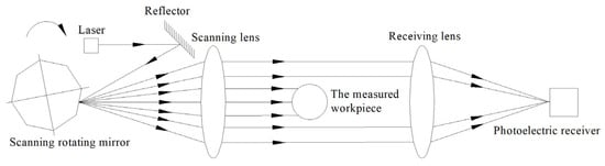
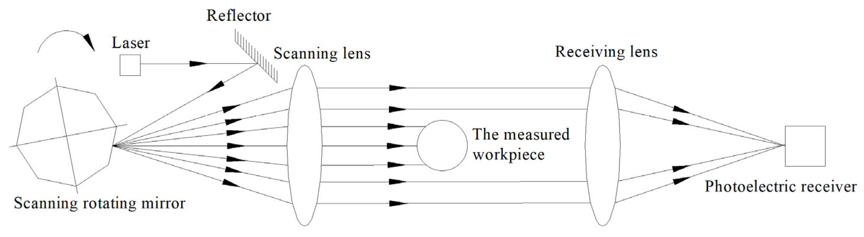
The structural principle of the laser scanning diameter measuring instrument is illustrated in Figure 1. A semiconductor laser emits a collimated ray that illuminates the polygonal scanner. A motor drives the polygonal scanner to rotate at a constant speed, causing the reflected ray to sweep across the f-theta lens at a constant angular velocity. The lens converts the reflected ray into one parallel to the optical axis, moving at a uniform speed to scan the workpiece under test. When the scanning ray is unobstructed by the workpiece, it is focused onto the photoelectric receiver through the receiving lens. The photoelectric receiver converts the optical signal into an electrical signal that varies over time, corresponding to the size of the workpiece. This signal is then processed by subsequent signal processing units to determine the workpiece’s dimensions [29].

Figure 1. Structural principle diagram of the laser scanning diameter measuring instrument.

2.2. Geometric Optical Model of the Polygonal Scanner System

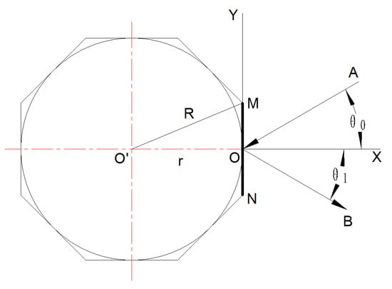
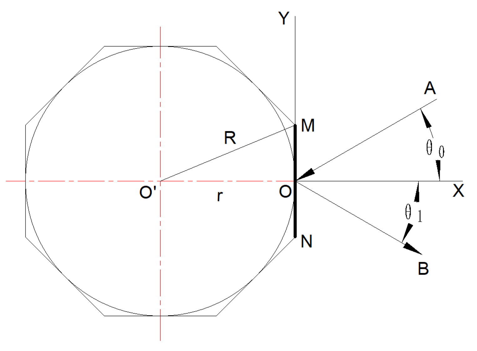
This article uses a regular octahedral polygonal scanner as an example to establish an analytical model. Its front projection is shown in Figure 2. The line segment MN represents the front projection of a specific side facet. The midpoint O of MN is taken as the coordinate origin to establish a two-dimensional coordinate system. The line containing MN is defined as the Y-axis, oriented upward. The line passing through point O and perpendicular to MN is defined as the X-axis, oriented positively to the right. In the figure, r denotes the radius of the inscribed circle of the regular octahedron, R denotes the radius of the circumscribed circle, and point O′ represents the rotation center of the polygonal scanner. When the laser ray reflection point is at point O, the line segment OA represents the incident ray, and the line segment OB represents the reflected ray. At this moment, the normal line coincides with the X-axis. Let the incident angle be ${\theta }_0$, such that ∠AOX = ∠BOX = ${\theta }_0$.

Figure 2. The reflection point is the center point O of the polygonal scanner.

Due to the geometric properties of a regular polyhedral scanner, it is sufficient to analyze the rotation characteristics of only one facet. Assume that the polygonal scanner rotates at a constant angular velocity, ω. After a time t, the line segment MN rotates to a specific position. At this time, the angle by which the polygonal scanner rotates away from the X-axis is ωt. A positive value of ωt corresponds to a counterclockwise rotation, while a negative value corresponds to a clockwise rotation. Let the drifting reflection point be E ($x,y$), and let the line segment EC represent the reflected ray when the reflection point drifts. The angle ${\theta }_1$ denotes the reflection angle.

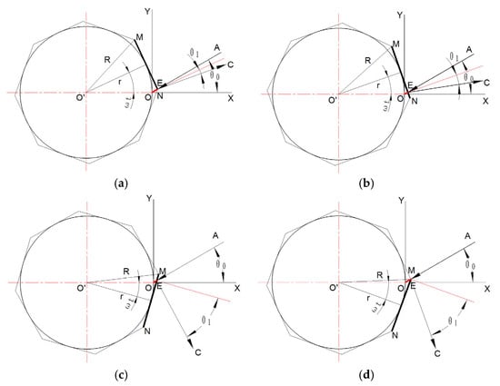
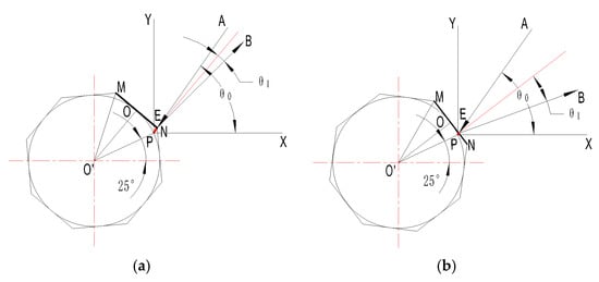
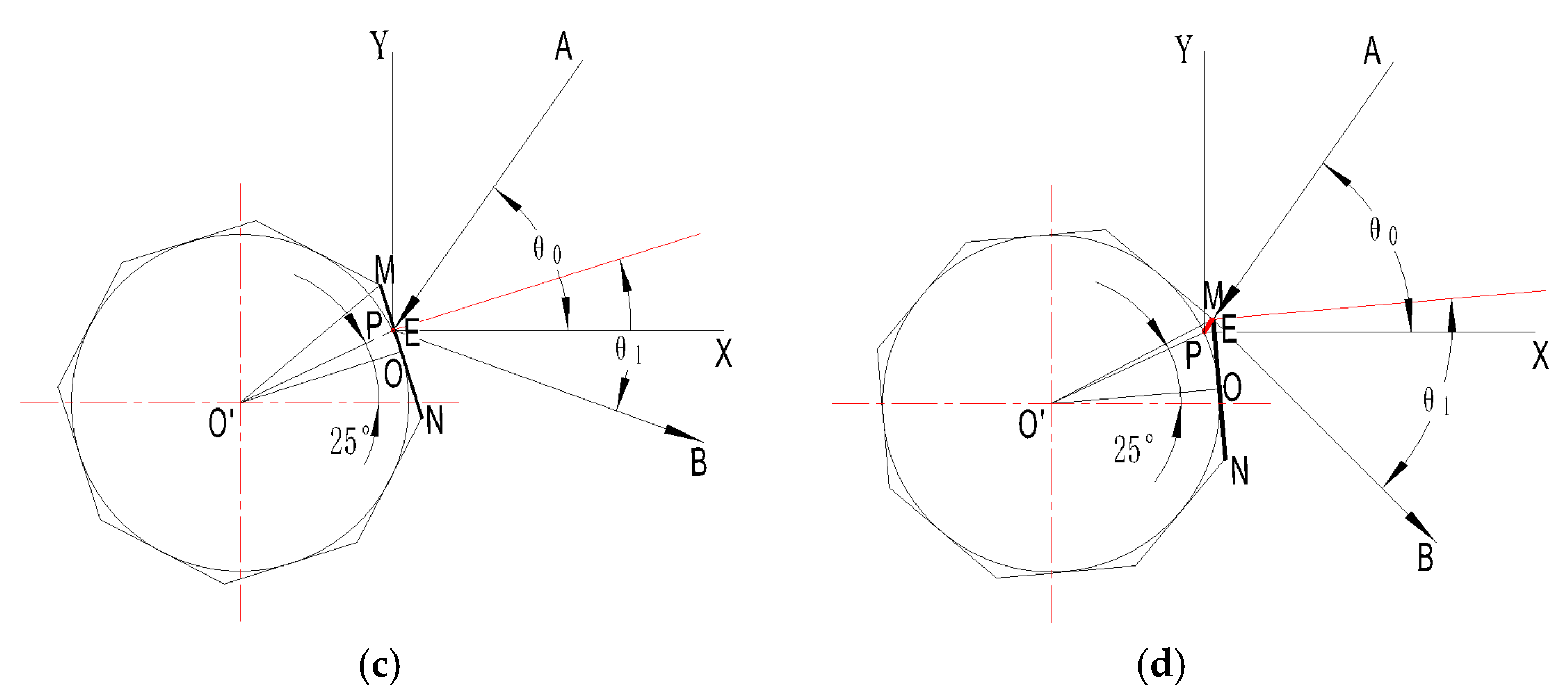
Using MN as an example, analyze the trajectory change of the reflection point as it moves from point N to point M when the polygonal scanner rotates clockwise. The characteristics shown in Figure 2 and Figure 3a–d correspond respectively to the trajectory changes when the reflection point is at point N, between points N and O, at point O, between points O and M, and at point M. The red line segment in the figure represents the reflection point drift. When the reflection point is at points N or M, its trajectory drifts to the farthest position, and the length of OE is calculated as the maximum distance traveled by the reflection point drift. When the reflection point is at point O, the trajectory converges to zero. As the reflection point moves from N to O—illustrated sequentially in Figure 2 and Figure 3a,b—the trajectory distance decreases from the maximum to zero. Conversely, as the reflection point moves from O to M—shown sequentially in Figure 2 and Figure 3c,d—the trajectory distance increases from zero to the maximum. The characteristics of the reflection point drift at any time t, as well as at points M and N, will be analyzed in detail later.

Figure 3. The characteristics of the reflection point drift on a certain facet. (a) The reflection point is at point N. (b) The reflection point lies between points N and O. (c) The reflection point lies between points O and M. (d) The reflection point is at point M.

2.3. Quantitative Analysis of the Reflection Point Drift in the Polygonal Scanner

2.3.1. The Reflection Point Lies Between Points O and M

When the reflection point lies between points O and M, the position of the reflection point drift at a given time t is shown in Figure 3c. According to the principles of geometric optics [30], the equation of the incident ray is:

$$y=x\tan {\theta }_0$$

(1)

When the rotation angle of the front projection line segment MN on a certain facet of the polygonal scanner is ωt, and assuming that the center point coordinates of the line segment MN are ($x_0,y_0$), its equation can be expressed as:

$$y-y_0=k_0(x-x_0)$$

(2)

$$\begin{array}{cc}\mathrm{in}:& x_0=-r(1-\cos \omega t),\hfill \\ & y_0=r\sin \omega t,\hfill \\ & k_0=\tan \left({\displaystyle \frac{\pi }{2}}-\omega t\right)=-\cot \omega t\hfill \end{array}$$

Enter the formula to obtain:

$$y=-x\cot \omega t+{\displaystyle \frac{r\left(1-\cos \omega t\right)}{\sin \omega t}}$$

(3)

The intersection point E ($x,y$) of the incident ray and the line segment MN, where the reflective surface is located, represents the coordinate of the reflection point drift. A system of linear equations is formed by combining formulas (1) and (3):

$$\left\{\begin{array}{c}y=x\tan {\theta }_0\\ y=-x\cot \omega t+{\displaystyle \frac{r(1-cos\omega t)}{sin\omega t}} \end{array}\right.$$

(4)

The coordinates of the reflection point drift are determined by solving the system of equations:

$$\left\{\begin{array}{c}x={\displaystyle \frac{r(1-\cos \omega t)}{\tan {\theta }_0\sin \omega t+\cos \omega t}}\\ y={\displaystyle \frac{r(1-\cos \omega t)\tan {\theta }_0}{\tan {\theta }_0\sin \omega t+\cos \omega t}}\end{array}\right.$$

(5)

According to the coordinate equation of the reflection point drift, it can be seen that this trajectory is actually a segment of the incident ray, that is, the line segment OE. The parameters ${\theta }_0$, ω, and r can be treated as constants, so the coordinates of the reflection point drift vary only with time t. Therefore, the trajectory can be expressed as a parametric equation in terms of t. Based on the geometric relationships, the behavior of the reflection point between points N and O also follows the same formula.

2.3.2. The Reflection Point Is at Point M

When the reflection point is at point M, the drift distance of the reflection point is greatest, corresponding to the length of OE, as shown in Figure 3d. Given the radius r of the inscribed circle and the number of faces n of the polygonal scanner, the radius of the circumscribed circle can be determined from the geometric relationships as follows:

$$\mathrm{R}={\displaystyle \frac{r}{\cos \frac{\pi }{n}}}$$

(6)

It is known that the initial incident angle is ${\theta }_0$. In triangle △OO′M′, the lengths of two sides are known to be r and R respectively, and one of the interior angles is $\mathrm{\angle }{\mathrm{O}}^{\prime }\mathrm{O}\mathrm{M}=\mathsf{\pi }-{\theta }_0$. Using the law of sines, the $\mathrm{\angle }\mathrm{O}{\mathrm{O}}^{\prime }\mathrm{M}$ and the length OE can be determined:

$$\mathrm{\angle }\mathrm{O}{\mathrm{O}}^{\prime }\mathrm{M}={\theta }_0-\mathrm{a}\mathrm{r}\mathrm{c}\sin (\sin {\theta }_0\cos {\displaystyle \frac{\pi }{n}})$$

(7)

$$OE=\mathrm{r}{\displaystyle \frac{\sin \left[{\theta }_0-arc\sin \left(\sin {\theta }_0\cos \frac{\pi }{n}\right)\right]}{\sin {\theta }_0\cos \frac{\pi }{n}}}$$

(8)

By combining the two formulas above, we can derive the following from the geometric relationship:

$${\omega t}_{min}=-{\displaystyle \frac{\pi }{n}}+{\theta }_0-\mathrm{a}\mathrm{r}\mathrm{c}\sin (\sin {\theta }_0\cos {\displaystyle \frac{\pi }{n}})$$

(9)

$${\omega t}_{max}={\displaystyle \frac{\pi }{n}}+{\theta }_0-\mathrm{a}\mathrm{r}\mathrm{c}\sin (\sin {\theta }_0\cos {\displaystyle \frac{\pi }{n}})$$

(10)

The length of the line segment OE represents the maximum displacement of the reflection point drift. From the geometric relationship, when the reflection point is at point M, the rotation angle reaches its minimum value, denoted as ${\omega t}_{min}$. Conversely, when the reflection point is at point N, the rotation angle attains its maximum value, denoted as ${\omega t}_{max}$. Therefore, the range of the rotation angle $\omega t$ is:

$$-{\displaystyle \frac{\pi }{n}}+{\theta }_0-arc\sin \left(\sin {\theta }_0\cos {\displaystyle \frac{\pi }{n}}\right)\le \omega t\le {\displaystyle \frac{\pi }{n}}+{\theta }_0-arc\sin \left(\sin {\theta }_0\cos {\displaystyle \frac{\pi }{n}}\right)$$

(11)

From the above calculation, it is evident that the number of faces n of the regular polyhedron, the radius of the inscribed circle r, and the initial incident angle ${\theta }_0$ determine the maximum distance of the reflection point drift as well as the range of the rotation angle. When these parameters are fixed, the maximum drift distance and the rotation angle range of the reflection point are also determined.

2.3.3. The Direction of Reflected Ray

As shown in Figure 2, when the reflection point is point O, the incident ray is OA, the reflected ray is OB, and the incident angle equals the reflected angle, both denoted as ${\theta }_0$. As shown in Figure 3, when the polygonal scanner rotates uniformly clockwise at the angular velocity ω, at any time t, the incident ray OA remains unchanged, and the reflected ray at that moment is EC. Assume that the incident angle at this time equals the reflected angle, denoted as ${\theta }_1$. According to geometric relationships:

$${\theta }_1={\theta }_0-\omega t$$

(12)

The angle between the reflected ray and the X-axis at this moment is:

$$\theta =2\omega t-{\theta }_0$$

(13)

From this, we can determine the slope of the reflected ray at time t:

$$k=\tan (2\omega t-{\theta }_0)$$

(14)

At this point, the calculation of the coordinates of the reflection point drift and the direction of the reflected ray has been completed. Given the initial incident angle ${\theta }_0$, the inscribed circle radius r and the number of faces n of the polygonal scanner, and the constant angular velocity ω, the specific values of x, y, and k can be determined at any time t. In other words, under these initial conditions, the drift characteristics of the reflection point can be established.

2.4. Analysis of the Reflection Point Drift When the Optical Axis Is Horizontal

The field of view angle corresponding to the regular octahedral polygonal scanner analyzed in Section 2.2 is 90°. The main optical axis of the scanning system should align with the bisector of the field of view. To analyze the measurement accuracy of the system, given the parameters of the polygonal scanner—specifically, the number of side facets n = 8 and the radius of the inscribed circle r = 10 mm—we initially let the incident ray strike the center of a particular facet, with an initial incident angle ${\theta }_0$ = 30°. The polygonal scanner rotates at a constant speed in a specified direction. The polygonal scanner is driven by a motor to rotate at a constant speed around its central axis. A positive value of ωt corresponds to a counterclockwise rotation, while a negative value corresponds to a clockwise rotation.

2.4.1. Geometric Optical Model of the Reflection Point Drift When the Optical Axis Is Horizontal

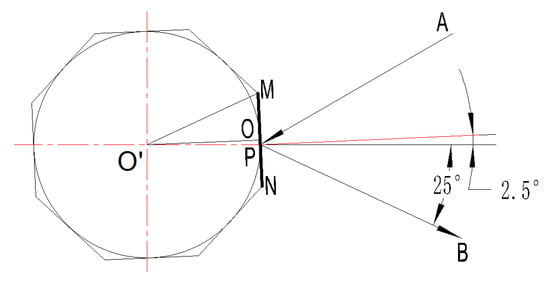
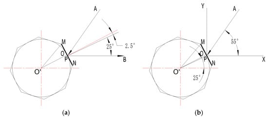
For the quantitative analysis in Section 2.3, according to formula (11), the value range of ωt is from −20° to 25°. According to formula (13), the angle between the reflected ray and the X-axis ranges from −70° to 20°. From this, it can be calculated that ωt = 2.5°, which corresponds to an angle of −25° between the reflected ray and the X-axis, serving as the main optical axis of the entire laser scanning system. Based on the geometric model of the polygonal scanner system shown in Figure 2, with the geometric center O′ of the polygonal scanner as the rotation center, the polygonal scanner can be rotated counterclockwise by 2.5°, as illustrated in Figure 4. At this position, the angle between the reflected ray and the X-axis is 25°. Based on the characteristics of the main optical axis of the laser scanning system, a new coordinate system is established with the incident point P as the origin, and the reflected ray PB aligned along the direction of the main optical axis.

Figure 4. The reflection point is point N.

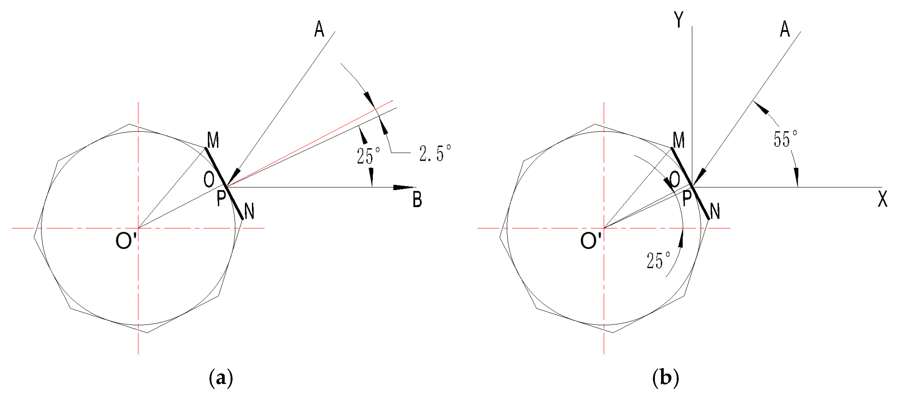
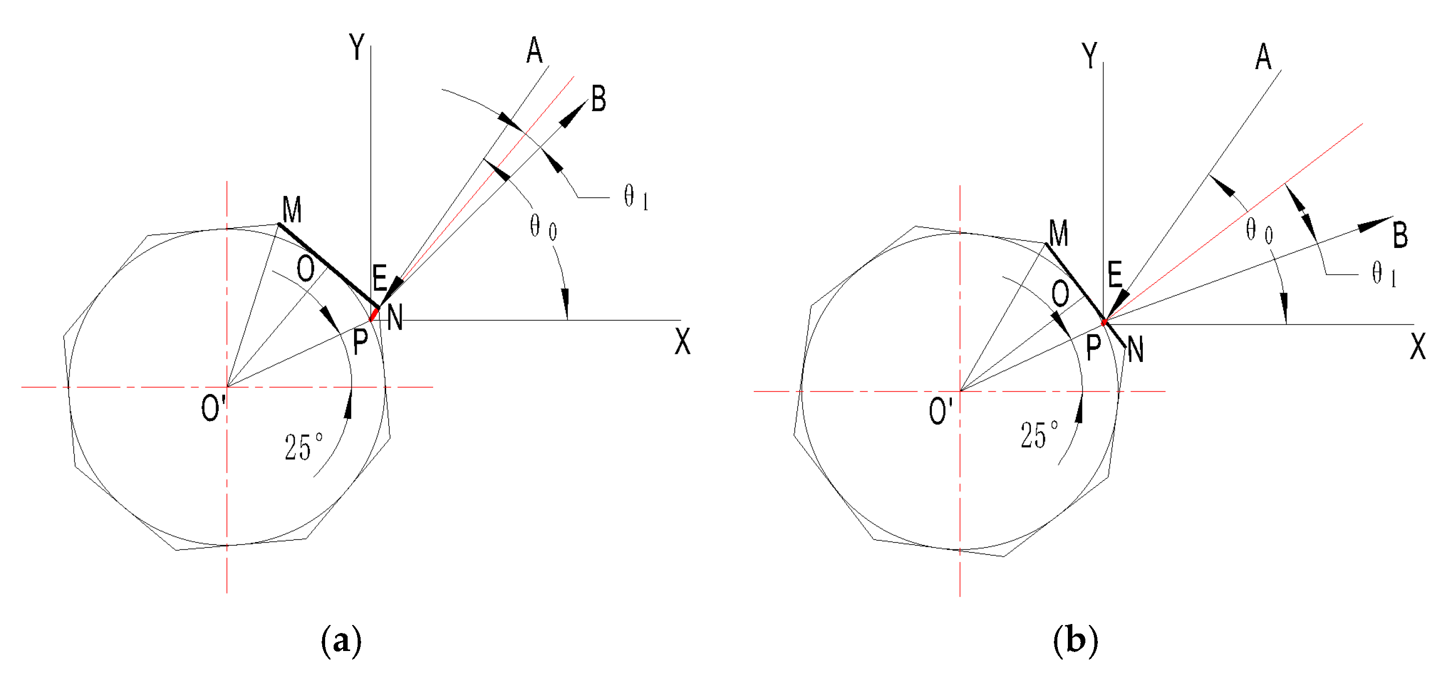
To align the optical axis horizontally, the polygonal scanner system is rotated counterclockwise by 25° around the incident point P, which serves as the center of rotation, based on the model shown in Figure 4. This adjustment is illustrated in Figure 5a, resulting in a new Cartesian coordinate system. In this model, point P is the origin, and the reflected ray PB defines the direction of the main optical axis, with the optical axis pointing to the right designated as the positive X-axis. The direction passing through point P and perpendicular to the optical axis is defined as the positive Y-axis. The incident angle at this position is 55°, as shown in Figure 5b.

Figure 5. Establishment of a coordinate system with a horizontal optical axis. (a) Rotate 25° counter clockwise around point P. (b) Create a new coordinate system with P as the origin.

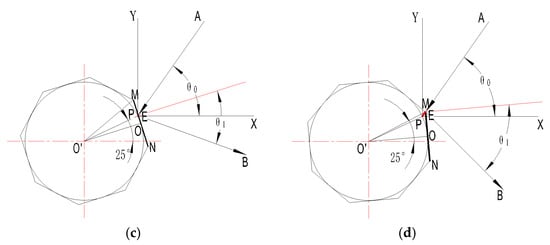
Similarly, using MN as an example, analyze the change of the reflection point drift as it moves from point N to point M during a clockwise rotation. The changes in the reflection point drift generally align with those described in Section 2.2, as shown in Figure 6.

Figure 6. The characteristics of the reflection point drift on a certain facet when the optical axis is horizontal. (a) The reflection point is at point N. (b) The reflection point lies between points N and O. (c) The reflection point lies between points O and M. (d) The reflection point is at point M.

2.4.2. Quantitative Analysis of the Reflection Point Drift with a Horizontal Optical Axis

Based on the geometric optical model of the polygonal scanner system described in 2.2, a coordinate transformation can be applied to derive a geometric optical model of the scanning system with a horizontal optical axis. In the original coordinate system, let point O have coordinates (0, 0) and point P have coordinates ($x_0$, $y_0$). Based on the geometric model of the polygonal scanner system, with the geometric center of the polygonal scanner as the rotation center, the polygonal scanner is rotated counterclockwise by 2.5°, and the coordinate origin shifts from point O to point P. First, the coordinates of point P can be obtained using formula (5):

$$\left\{\begin{array}{c}{x}_0={\displaystyle \frac{r(1-\cos 2.5°)}{\tan {\theta }_0\sin 2.5°+\cos 2.5°}}\\ y_0=x_0\tan {\theta }_0\end{array}\right.$$

(15)

According to the law of shifting the axis during coordinate transformation in a rectangular coordinate system, the coordinates of the center point of the polygonal scanner change from (−r, 0) to ($-r-x_0$, ${-y}_0$).

After the coordinate transformation and axis shift, the coordinates of the reflection point drift E (x, y) become:

$$\left\{\begin{array}{c}x={\displaystyle \frac{r(1-\cos \omega t)}{\tan {\theta }_0\sin \omega t+\cos \omega t}}-x_0\\ y={\displaystyle \frac{r(1-\cos \omega t)\tan {\theta }_0}{\tan {\theta }_0\sin \omega t+\cos \omega t}}{-y}_0\end{array}\right.$$

(16)

Next, take the incident point P as the center of rotation and rotate the entire system counterclockwise by 25°. According to the rules for the rotation axis during coordinate transformation in a rectangular coordinate system, the coordinates of the polygonal scanner center point O′ (x′, y′) become:

$$\left\{\begin{array}{c}{x}^{\prime }=-(r+x_0)\mathit{cos}25°+y_0\sin 25°\\ y^{\prime }=-(r+x_0)\sin 25°-y_0\cos 25°\end{array}\right.$$

(17)

After the coordinate transformation of the axis, the coordinates of the reflection point drift E (x, y) become:

$$\left\{\begin{array}{c}x=\left({\displaystyle \frac{r(1-\cos \omega t)}{\tan {\theta }_0\sin \omega t+\cos \omega t}}-x_0\right)\cos 25°-\left({\displaystyle \frac{r(1-\cos \omega t)\tan {\theta }_0}{\tan {\theta }_0\sin \omega t+\cos \omega t}}-y_0\right)\sin 25°\\ y=\left({\displaystyle \frac{r(1-\cos \omega t)}{\tan {\theta }_0\sin \omega t+\cos \omega t}}-x_0\right)\sin 25°+\left({\displaystyle \frac{r(1-\cos \omega t)\tan {\theta }_0}{\tan {\theta }_0\sin \omega t+\cos \omega t}}-y_0\right)\cos 25°\end{array}\right.$$

(18)

When the reflection point is at point M or point N, the drift amount is greatest. The calculation and analysis follow the same procedure as described in Section 2.3.2.

Considering the direction of the reflected ray from the model, the angle between the reflected ray and the X-axis, based on the geometric relationship, is:

$$\theta =2\omega t-2\times 2.5°$$

(19)

The slope of the reflected ray at time t can be determined as follows:

$$k=\tan (2\omega t-2\times 2.5°)$$

(20)

3. Analysis and Discussion

3.1. Simulation of the Reflection Point Drift and the Direction of the Reflected Ray

Use simulation software Matlab2016 to verify the results of the previous analysis by simulating the changes in the coordinates of the reflection point drift and the direction of the reflected ray. This primarily serves to verify and analyze the results of Section 2.4.

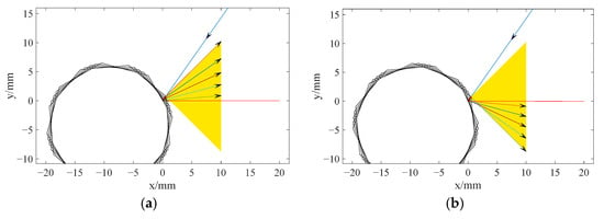
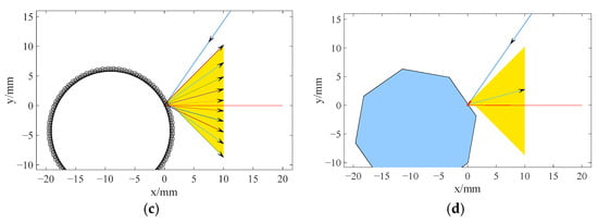
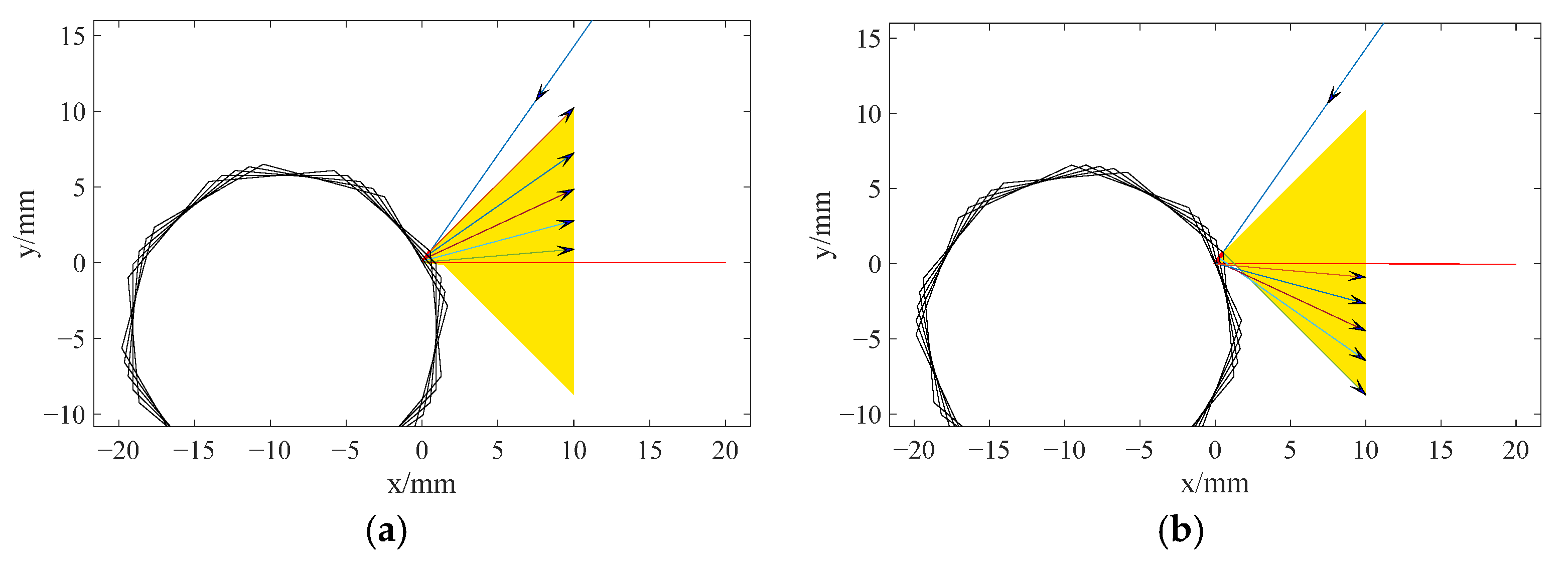
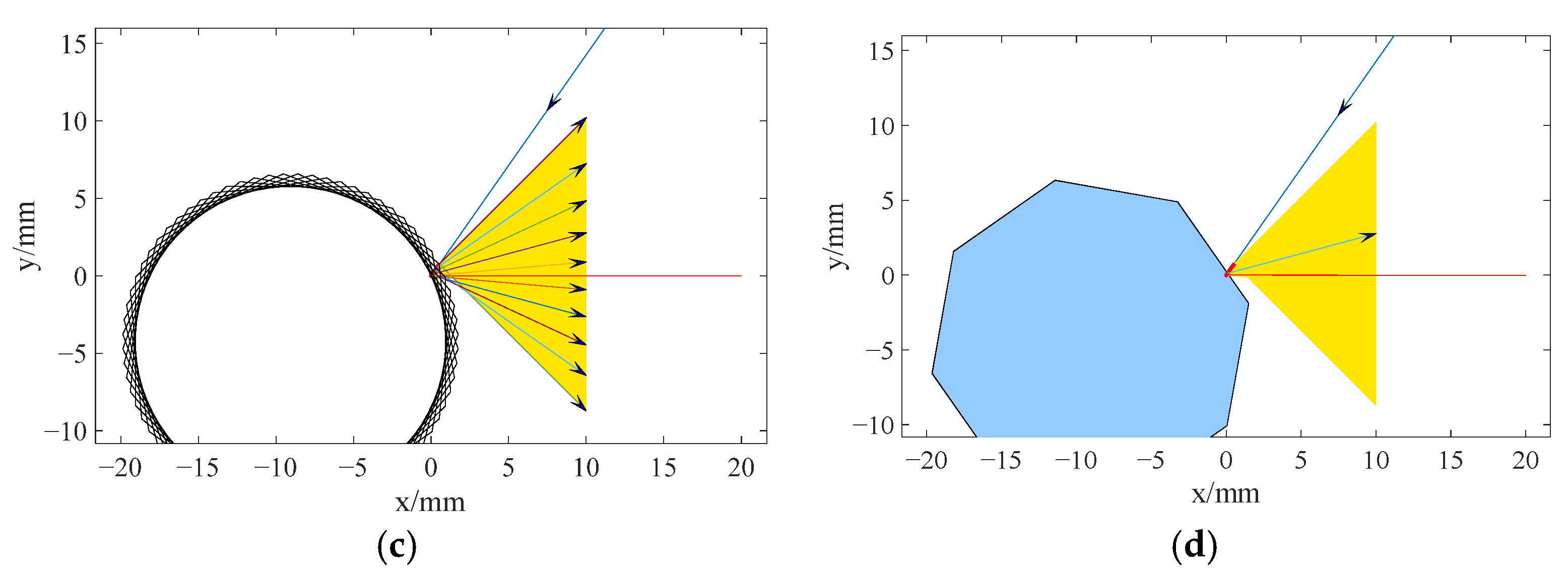
Figure 7 presents the output of the simulation of reflection point drift and reflected ray. Figure 7a illustrates the change in the direction of the reflected ray when the incident ray is projected onto the lower half of facet ON as the polygonal scanner rotates counterclockwise at an angular velocity of ωt. According to the law of reflection, when $\omega t=2.5°$, the reflection point does not drift, and it is exactly at point P as shown in Figure 5b, where the angle between the reflected ray and the X-axis is 0°. According to the formula (10), when ${\omega t}_{min}=-22.5°$, the reflection point drifts to its farthest position at point N in Figure 6a, where the angle between the reflected ray and the X-axis is 45°. Figure 7b illustrates the change in the direction of the reflected ray when the incident ray is projected onto the upper half of facet OM, as the polygonal scanner rotates clockwise at speed ωt. According to formula (9), when ${\omega t}_{min}=-22.5°$, the reflection point drifts to its farthest position at point M in Figure 6d, where the angle between the reflected ray and the X-axis is −45°. Figure 7c depicts the changes in the reflection point drift and the direction of the reflected ray when the incident ray is projected onto the entire facet containing segment MN, as the polygonal scanner rotates at speed ωt. This figure combines the results shown in Figure 7a,b. The reflection point drift pattern on the complete reflecting facet first gradually decreases from the farthest position to zero, then gradually increases from zero back to the farthest position. When the reflection point is at point O, the drift amount is zero; when at points N and M, the drift amount reaches its maximum, according to formula (8) and the known conditions in Section 2.4, and the maximum drift amount calculation yields an approximate value of 1. Figure 7d illustrates the changes in the reflection point drift and the direction of the reflected ray at a specific reflection point.

Figure 7. Simulation of the reflection point drift and the reflected ray. (a) The reflection point lies between points N and O. (b) The reflection point lies between points O and M. (c) The reflection point is on the entire facet containing segment MN. (d) A specific reflection point. In the figure: The yellow area represents the field of view range. The blue ray outside the yellow area is the incident ray, while the rays within the yellow area are the reflected lights from different incident angles. The red line represents the main optical axis.

According to formula (11), the value of ωt ranges from −22.5° to 22.5°, and the angle between the reflected ray and the X-axis ranges from −45° to 45°. The simulation results are fully consistent with the previous theoretical analysis.

3.2. Analysis of the Impact of the Reflection Point Drift on Measurement Accuracy

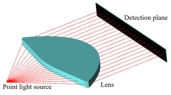
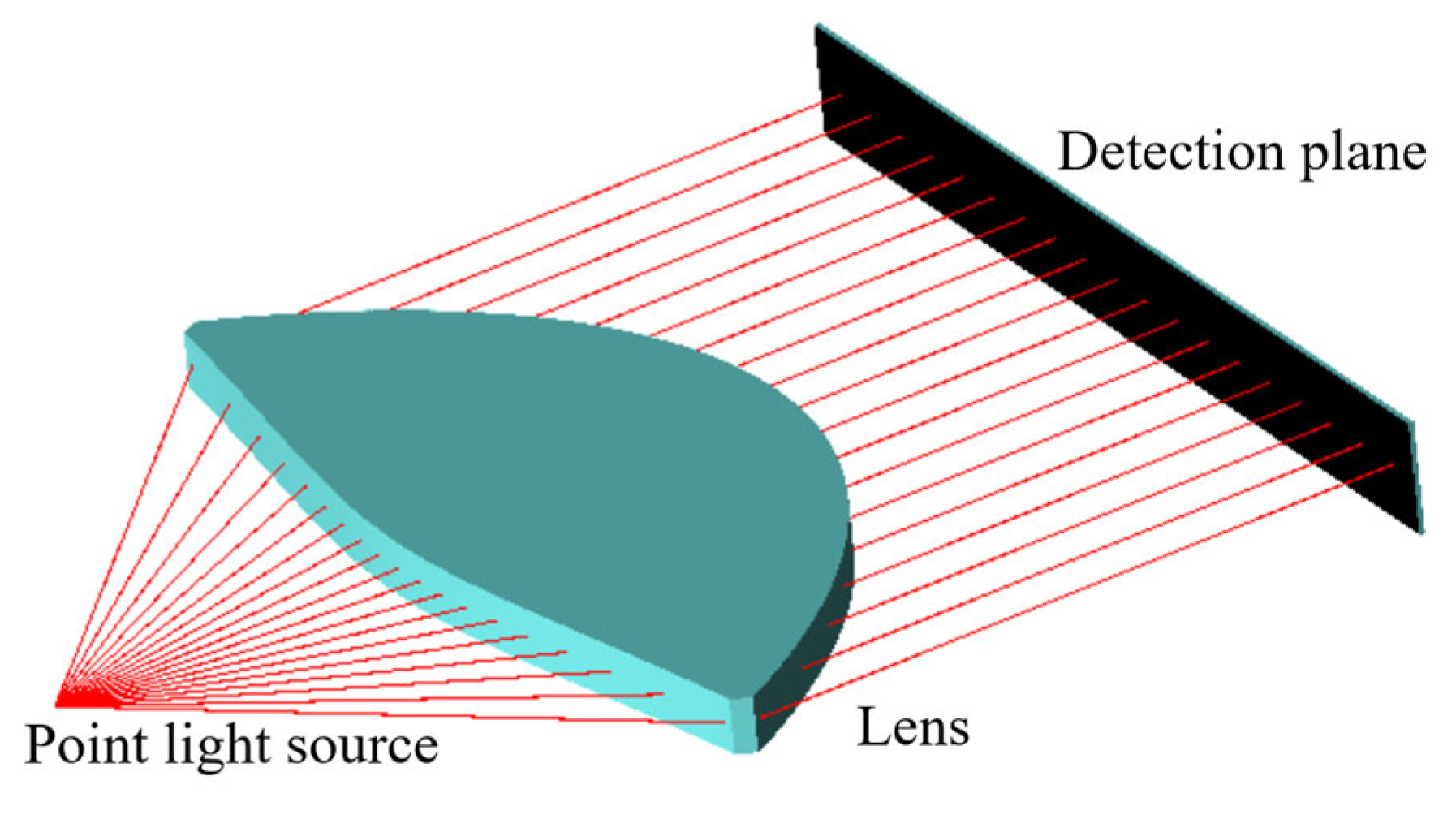
The field of view angle corresponding to the regular octahedral polygonal scanner analyzed in Section 2.2 is 90°. First, an ideal scenario is simulated where the reflection point of the laser ray incident on the polygonal scanner is fixed. In this case, the point light source can be positioned at the reflection point, allowing the polygonal scanner to be disregarded. In optical simulation software Zemax2009, a point light source, a double freeform surfaces f-theta lens with a 90° field of view, and a detection surface are configured to form a laser scanning system. The parameters of this system can be set to various parameter settings for an angle of field of 90° lens, as described in Reference [31]. The detection plane is also the focal plane of the f-theta lens. The detection plane distance from the origin is set at 200 mm. This value is based primarily on the preset parameters of an f-theta lens: focal length f = 100 mm, object distance L = 64.6 mm, and lens thickness d = 71.6 mm. Multiple rays with varying tilt angles are emitted from the point light source and directed onto the f-theta lens to simulate the optical transformation effect of a fixed reflection point, as shown in Figure 8. The ray projection position on the detection surface is observed to evaluate the distortion of the optical transformation. It is found that the absolute value of the measured absolute distortion is less than 0.2 mm, and the absolute value of the relative distortion is less than 1%. According to research [31], the magnitude of the lens scanning linearity error is fully controllable and is primarily determined by the discrete angle. Provided the computer hardware permits, continuously reducing the discrete angle can further decrease the relative distortion to meet the design requirement of 0.5–0.1%. This also demonstrates the superior performance of the double freeform surfaces’ f-theta lens.

Figure 8. Optical transformation effect of the fixed reflection point.

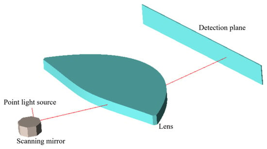
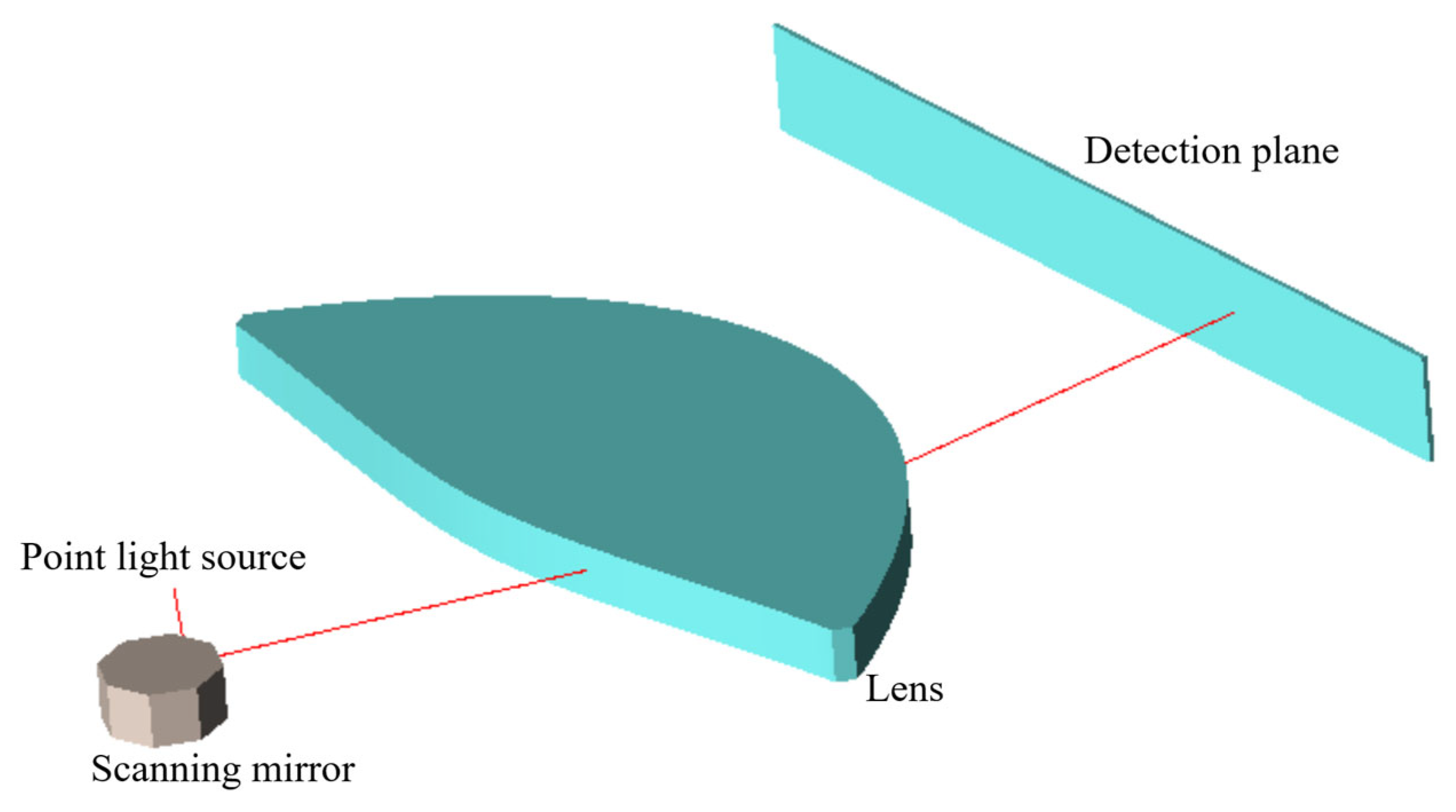
To simulate the impact of reflection point drift on measurement accuracy, a new laser scanning system was developed using optical simulation software. A polygonal scanner was added to the model shown in Figure 8, and the position of the point light source was adjusted. The rays, reflected by the polygonal scanner at various tilt angles, were directed onto the double freeform surfaces’ f-theta lens with a 90° field of view. This setup simulated the optical transformation under conditions of reflection point drift, as illustrated in Figure 9.

Figure 9. Optical transformation effect of the reflection point drift. The red lines represent the optical path.

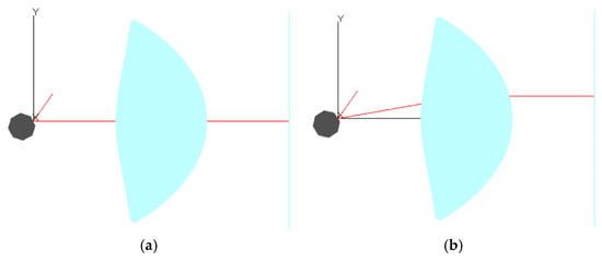
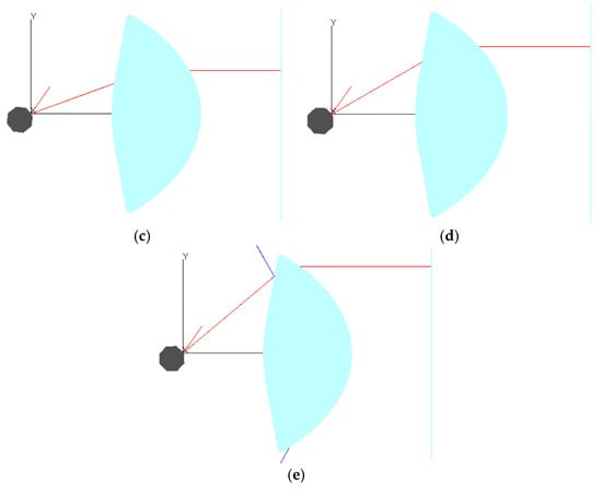
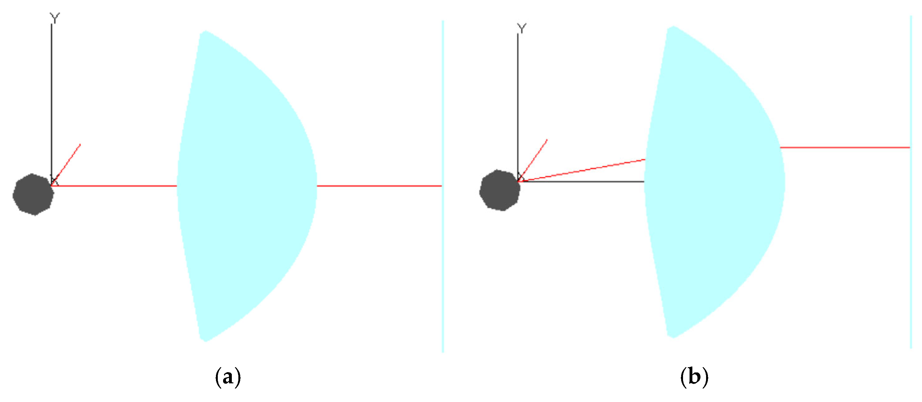
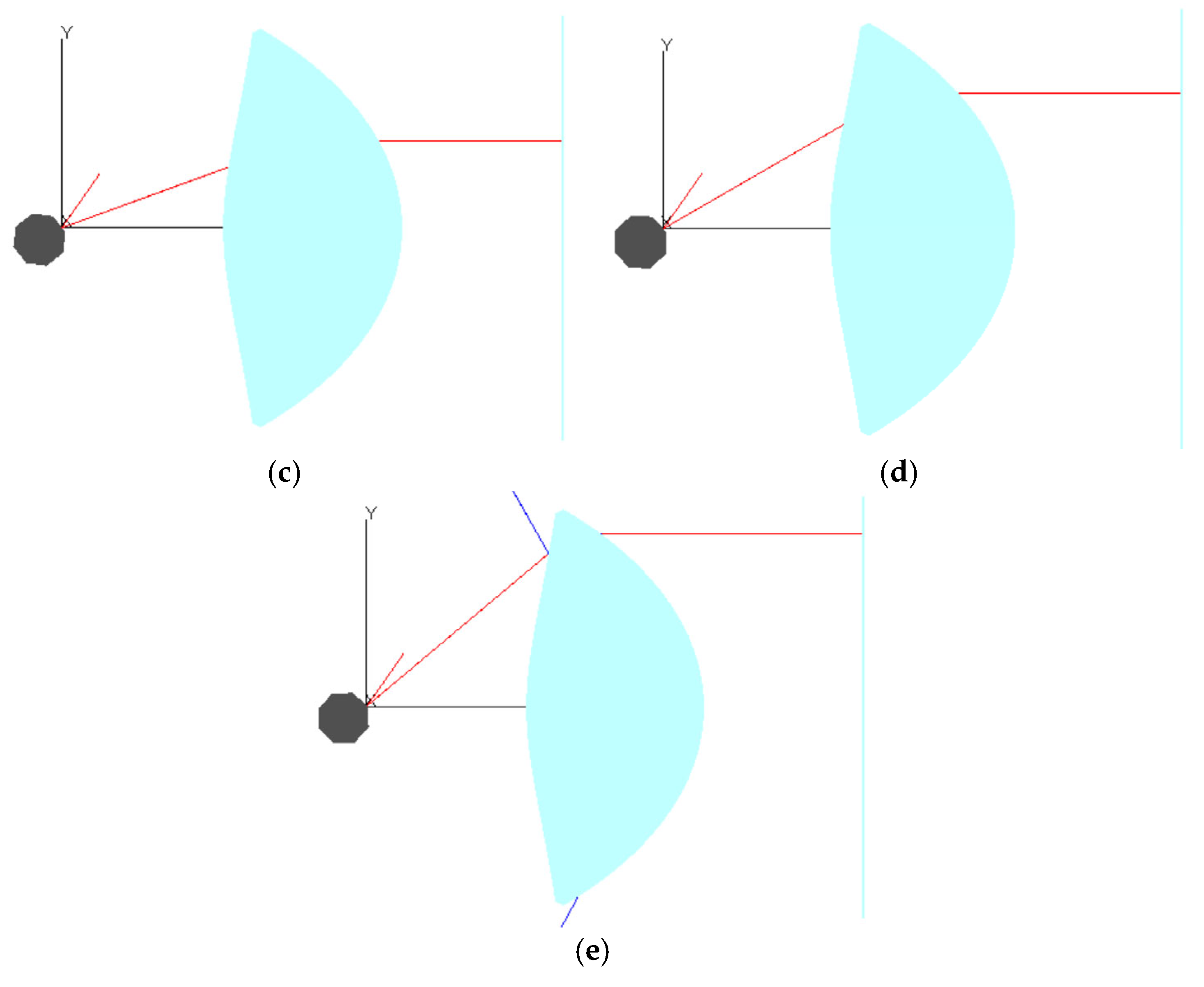
When the polygonal scanner rotates to different angles, the reflection point drifts to different positions, causing the position and direction of the reflected ray to deviate from the preset trajectory. Figure 10 shows the meridian path diagrams of rays for different incident angles θ based on the model in Figure 9.

Figure 10. The meridian path diagrams of rays for different incident angles θ: (a) θ = 0°; (b) θ = 10°; (c) θ = 20°; (d) θ = 30°; and (e) θ = 40°.

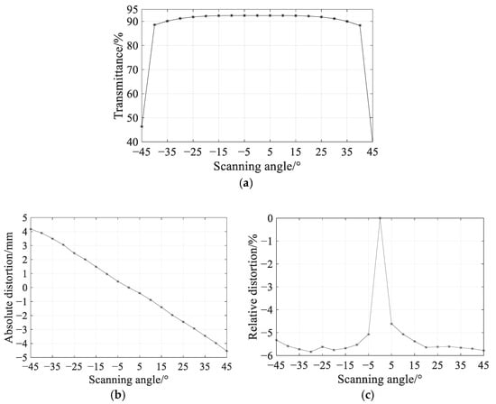
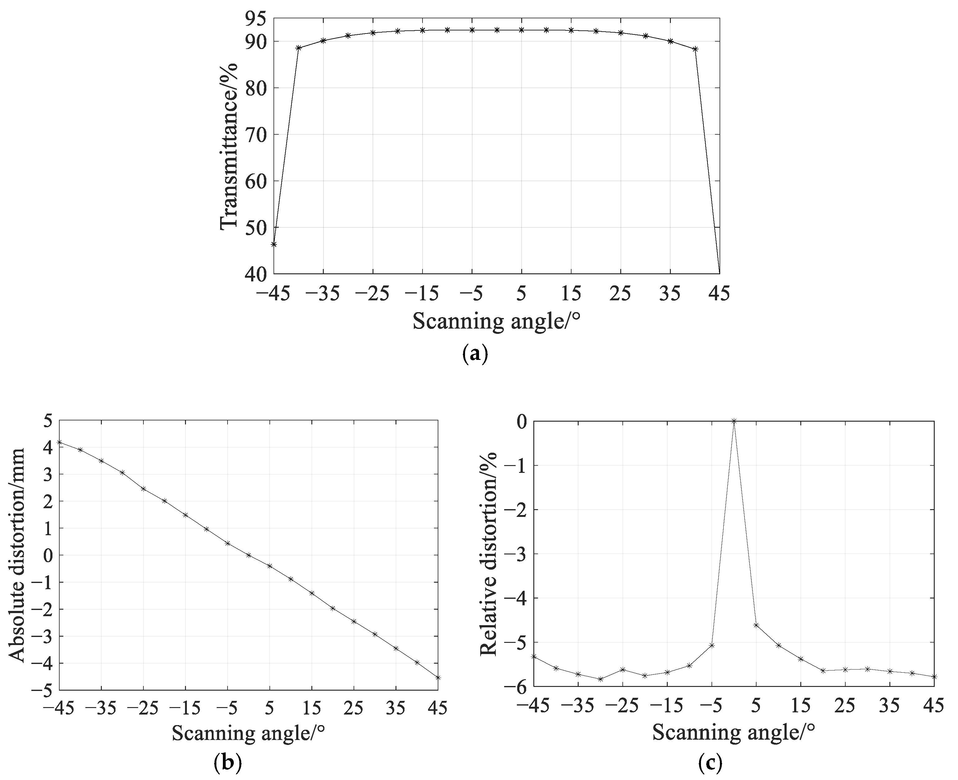
The recorded data indicate that under the conditions of reflection point drift, the measured transmittance values ranged from a high of 92.429% to a low of 39.447%. The absolute distortion reached up to −4.54 mm, while the relative distortion was as high as −5.83%, as shown in Figure 11. Compared to the ideal state data [31], transmittance is significantly reduced at the edge of the lens; absolute distortion increases by nearly 20 times, and relative distortion increases by nearly 5 times. These results demonstrate that reflection point drift has a substantial impact on measurement accuracy.

Figure 11. The variation in measurement accuracy during the reflection point drift. (a) The transmittance varies with the scanning angle. (b) The absolute distortion varies with the scanning angle. (c) The relative distortion varies with the scanning angle.

4. Discussion

Based on a geometric optics model, this article quantitatively analyzes the reflection point drift and the direction of the reflected ray caused by the rotation of a polygonal scanner, as well as the impact of this drift on measurement accuracy. Using the polygonal scanner in a laser scanning diameter measuring instrument as the research subject, a geometric model is established. Taking a regular octahedral polygonal scanner as an example, we quantitatively analyze the reflection point drift on a specific prism face and the directional changes of the reflected ray when the polygonal scanner rotates at a constant speed. This study shows that, under certain initial conditions, the reflection point drift and the direction of the reflected ray vary only with time t.

According to the design requirement that the main optical axis of the scanning system be horizontal, and using the principle of coordinate transformation, a model of the coordinates of the reflection point drift and the direction of the reflected ray when the optical axis is horizontal is established. The impact of drift on the measurement accuracy is then quantitatively analyzed. The research shows that, compared to the ideal state, the reflection point drift causes the system’s absolute distortion to increase by nearly 20 times and the relative distortion to increase by nearly 5 times, indicating that the reflection point drift significantly affects the measurement accuracy.

In summary, the model of the reflection point drift and the direction of the reflected ray proposed in this article is simple, efficient, and easy to understand, with a wide range of applications. Future research can directly incorporate this quantitative analysis model into the design of relevant f-theta lenses, effectively and conveniently enhancing lens design accuracy, thereby improving the overall measurement precision of the system. This research holds significant theoretical importance and engineering value in advancing the application of laser scanning technology in high-precision measurements, micro-nano manufacturing, and other fields.

References

- Yao, C.W.; Han, Y.C.; Zhou, P.; Wang, H.Y.; Wang, Y.; Lin, B. Mirror-assisted 360° panoramic 3D measurement system based on rotary laser profilometer. Meas. Sci. Technol. 2024, 35, 095206. [Google Scholar] [CrossRef] [Scilit]
- May, K.H.; Mohammadzadeh, S.; Keil, A.; von Freymann, G.; Friederich, F. Coherent Off-Axis Terahertz Tomography with a Multi-Channel Array and f-theta Optics. Sensors 2024, 24, 529. [Google Scholar] [CrossRef] [Scilit] [PubMed]
- Zhou, H.; Mao, Q.Z.; Song, Y.F.; Wu, A.L.; Hu, X.Q. Analysis of Internal Angle Error of UAV LiDAR Based on Rotating Mirror Scanning. Remote Sens. 2022, 14, 5260. [Google Scholar] [CrossRef] [Scilit]
- Kazuo, M. Historical Review and Future Trends of Scanning Optical Systems for Laser Beam Printers. Proc. SPIE 1993, 1987, 264–273. [Google Scholar] [CrossRef] [Scilit]
- Kim, W.-B.; Moon, S.-D.; Yoo, J.-H.; Kim, H.-C. Optical design and manufacturing technology for high resolution laser scanning unit. Int. J. Precis. Eng. Man. 2009, 10, 141–146. [Google Scholar] [CrossRef] [Scilit]
- Duma, V.-F.; Podoleanu, A.G. Polygon mirror scanners in biomedical imaging: A review. Proc. SPIE 2013, 8621, 175–183. [Google Scholar] [CrossRef] [Scilit]
- Ikari, T.; Sasaki, Y.; Otani, C. 275-305 GHz FM-CW Radar 3D Imaging for Walk-Through Security Body Scanner. Photonics 2023, 10, 343. [Google Scholar] [CrossRef] [Scilit]
- Wang, Y.H.; Yi, L.; Tonouchi, M.; Nagatsuma, T. High-Speed 600 GHz-Band Terahertz Imaging Scanner System with Enhanced Focal Depth. Photonics 2022, 9, 913. [Google Scholar] [CrossRef] [Scilit] [PubMed]
- Duma, V.-F. Analysis of polygonal mirror scanning heads: From industrial to high-end applications in swept sources for OCT. Proc. SPIE 2017, 100560, 121–131. [Google Scholar]
- Duma, V.F.; Duma, M.A. Optomechanical analysis and design of polygon mirror-based laser scanners. Appl. Sci. 2022, 12, 5592. [Google Scholar] [CrossRef] [Scilit]
- Duma, V.-F.; Rolland, J.P. Mechanical Constraints and Design Considerations for Polygon Scanners. Mech. Mach. Sci. 2010, 5, 475–483. [Google Scholar] [CrossRef] [Scilit]
- Duma, V.F. Polygonal Mirror Laser Scanning Heads: Characteristic Functions. Proc. Rom. Acad. Ser. A 2017, 18, 25–33. [Google Scholar]
- Hoang, H.M.; Choi, S.; Park, C.; Choi, J.; Ahn, S.H.; Noh, J. Non-back-reflecting polygon scanner with applications in surface cleaning. Opt. Express 2021, 29, 32939. [Google Scholar] [CrossRef] [Scilit] [PubMed]
- Pernechele, C.; Consolaro, L.; Jones, G.H.; Brydon, G.; Da Deppo, V. Telecentric F-theta fisheye lens for space applications. OSA Contin. 2021, 4, 783–789. [Google Scholar] [CrossRef] [Scilit]
- Zhou, Q.; Tian, Y.; Wang, J.; Xu, M. Design and implementation of a high-performance panoramic annular lens. Appl. Opt. 2020, 59, 11246–11253. [Google Scholar] [CrossRef] [Scilit] [PubMed]
- Novák, J.; Mikš, A. Method for algebraic calculation of initial design parameters of a two-element telecentric f-theta lens. Appl. Opt. 2023, 62, 6113–6119. [Google Scholar] [CrossRef] [Scilit] [PubMed]
- Wang, W.; Schmidt, K.; Wapler, M.C.; Wallrabe, U.; Czarske, J.W.; Koukourakis, N. Fully refractive telecentric f-theta microscope based on adaptive elements for 3D raster scanning of biological tissues. Opt. Express 2023, 31, 29703–29715. [Google Scholar] [CrossRef] [Scilit] [PubMed]
- Chen, C.; Pu, Y.; Shi, W. Low-cost spectrometer design for ultra-high resolution spectral domain optical coherence tomography. Chin. Opt. Lett. 2023, 21, 101101. [Google Scholar] [CrossRef] [Scilit]
- Qiu, T.; Lou, Y.; Yan, L.; Xie, J.; Zhao, D.; Hu, M.; Chen, B. System error modeling and precision compensation in rotating-mirror laser trackers. Opt. Lasers Eng. 2025, 195, 109259. [Google Scholar] [CrossRef] [Scilit]
- Han, W.H.; Lee, S.W.; Lim, J.; Park, N.C.; Kim, W.C. Design and feasibility study on a compact wide-field LiDAR optical system using polygonal mirrors. Opt. Lasers Eng. 2025, 195, 109273. [Google Scholar] [CrossRef] [Scilit]
- Faitli, T.; Hyyppä, E.; Hyyti, H.; Hakala, T.; Kaartinen, H.; Kukko, A.; Muhojoki, J.; Hyyppä, J. Integration of a Mobile Laser Scanning System with a Forest Harvester for Accurate Localization and Tree Stem Measurements. Remote Sens. 2024, 16, 3292. [Google Scholar] [CrossRef] [Scilit]
- Altyntsev, M.A. Relative Adjustment of Mobile Laser Scanning Data in Different Scenes. Isprs Ann. Photo Rem. 2022, 5-1, 111–120. [Google Scholar] [CrossRef] [Scilit]
- Yuan, H.L.; Zhang, H.; Zha, B.T.; Ding, L.B. Trajectory correction and position error analysis of underwater laser scanning. Opt. Laser Technol. 2022, 153, 108136. [Google Scholar] [CrossRef] [Scilit]
- Keitaanniemi, A.; Rönnholm, P.; Kukko, A.; Vaaja, M.T. Drift analysis and sectional post-processing of indoor simultaneous localization and mapping (SLAM)-based laser scanning data. Autom. Constr. 2023, 147, 104700. [Google Scholar] [CrossRef] [Scilit]
- Zhai, Y.S.; Wu, R.X.; Zhang, R.L.; Yang, H.J.; Yang, P.; Li, S.; Zhang, Z.F. Real-time laser detection method for edge position of objects with nanometer level accuracy. Appl. Opt. 2025, 64, 10701–10709. [Google Scholar] [CrossRef] [Scilit] [PubMed]
- Liu, L.E.; Zhang, Y.X.; Wang, N.; Tang, L.; Yan, C.Y.; Zhou, J.L.; Gao, W.J.; Zhang, Y.F.; Lv, J.X.; Zhang, Z. Image drift compensation in scanning electron microscopy facilitated by an external scanning and imaging system. Micron 2025, 196, 103848. [Google Scholar] [CrossRef] [Scilit] [PubMed]
- Li, J.K.; Han, S.; Zhao, B.T.; He, Q.X.; Hu, K.F.; Qian, Y.B.; Feng, Q.B. Method and Compensation Model for Measuring Geometric Errors of Rotary Axis Based on Circular Grating. IEEE Sens. J. 2025, 25, 40727–40737. [Google Scholar] [CrossRef] [Scilit]
- Marshall, G.F.; Stutz, G.E. Handbook of Optical and Laser Scanning, 2nd ed.; CRC Press/Taylor & Francis Group: Boca Raton, FL, USA, 2012; pp. 70–132. [Google Scholar]
- Benner, W.R. Laser Scanners: Technologies and Applications; Pangolin Laser Systems, Inc.: Sanford, FL, USA, 2016. [Google Scholar]
- Born, M.; Wolf, E. Principle of Optics, 7th ed.; World Publishing Corporation: Cleveland, OH, USA, 2001. [Google Scholar]
- Wang, L.; Chen, K.; Kang, X.; Zheng, H. Numerical Iterative Design and Analysis of Double Freeform Surface Telecentric F-Theta Lens. Sensors 2025, 25, 4949. [Google Scholar] [CrossRef] [Scilit] [PubMed]
Disclaimer/Publisher’s Note: The statements, opinions and data contained in all publications are solely those of the individual author(s) and contributor(s) and not of MDPI and/or the editor(s). MDPI and/or the editor(s) disclaim responsibility for any injury to people or property resulting from any ideas, methods, instructions or products referred to in the content. |
© 2026 by the authors. Licensee MDPI, Basel, Switzerland. This article is an open access article distributed under the terms and conditions of the Creative Commons Attribution (CC BY) license.