


Abstract
In time-delay reservoir computing (TDRC), mask signal generation techniques in the input layer remain a key factor limiting system integration. In this study, we propose an optical mask generation scheme based on steady–quasi-periodic state switching (S-QPS) dynamics in a semiconductor laser with optical feedback. Experimentally generated S-QPS signals are applied to a TDRC system as mask signals, and the system performance is evaluated using the Santa Fe chaotic time-series prediction task. S-QPS signals are numerically generated based on the Lang–Kobayashi rate equations. The optimal normalized mean square error is 0.027. An analysis of the factors affecting system performance is carried out. The results indicate that period offset has a limited impact on system performance. In contrast, noise-induced amplitude fluctuations have a more pronounced impact. These results provide insights into the use and optimization of S-QPS signals for optical mask generation in TDRC systems.
1. Introduction
Reservoir computing is a simplified recurrent neural network in which only the output weights need to be trained [1,2,3], and it has been widely applied in time-series prediction, speech recognition, and financial forecasting [4,5,6]. Subsequently, time-delay reservoir computing (TDRC) replaces multiple physical nodes using a single nonlinear node with a delayed feedback loop, significantly reducing hardware implementation complexity [7,8,9]. Thus, TDRC has attracted widespread attention and research interest.
A typical TDRC system consists of three parts: an input layer, a reservoir layer, and an output layer. With the assistance of appropriate optical and electronic auxiliary modules, the reservoir and output layers can achieve a high degree of hardware integration [10,11,12,13,14,15,16]. Meanwhile, the technique of mask generation restricts the integration of the input layer, thereby hindering the hardware implementation of TDRC systems. As an indispensable component of the input layer, the mask induces complex transient responses and enhances the computational capability of the TDRC system [17]. Previous studies on mask signal mainly focused on the influence of different mask formats on the performance of TDRC, such as optimized binary [18], six-level [19], chaotic [20], or colored-noise [17] mask signals. To meet the requirements for periodicity and sufficient intra-period numerical diversity in the mask signal, most TDRC schemes have relied on high-bandwidth arbitrary waveform generators (AWG) to generate mask signals, which are costly and functionally redundant. With the continuous maturation of TDRC and related hardware technologies, researchers urgently need to explore the generation of the mask signal to promote the TDRC system integration. Specifically, the all-optical mask signal will be seamlessly integrated with photonic TDRC for high-speed information processing.
In 2016, Duport et al. demonstrated that mask signals could be generated by feeding two continuous-wave radio frequency (RF) tones into a modulator [21]. In 2021, Argyris et al. generated quasi-sinusoidal signals using a semiconductor laser with optical feedback (SL-OF) and produced mask signals by adjusting the strengths of different frequency components in the microwave domain through multiple electrical amplifiers [22]. Subsequently, Yue et al. realized mask generation in 2022 and 2024 by combining a mode-locked laser with dispersion elements, realizing it in an optical spectral filter and a Mach–Zehnder interferometer or a three-section fiber structure, respectively [23,24]. In 2025, Chen et al. utilized a sinusoidal signal to modulate the pump current of the SL-OF to generate periodic complex signals as mask signals [25]. Meanwhile, Bauwens et al. designed a space-time hybrid TDRC architecture, in which the input masking function is implemented using a passive spatially distributed photonic network [26]. However, the complexity of the device and the slow cycle of the mask limit the processing speed of the TDRC. On the other hand, researchers have attempted to design mask-free TDRC architectures in order to bypass the difficulty of mask generation [27,28], but the generality still needs to be discussed. Therefore, exploring efficient mask generation schemes continues to be a key issue in current research for TDRC.
We find that the “steady–quasi-periodic state switching” (S-QPS) dynamic states noticed by Dong et al. in the SL-OF system [29,30] are highly consistent with the fundamental requirements of mask signals. The S-QPS behavior has been verified through both experiments and numerical simulations in multiple types of semiconductor laser [31,32,33]. The controllable periodicity and rich numerical diversity within their quasi-periodic segments have motivated us to explore the S-QPS signal as a mask in TDRC systems to replace the conventional AWG-based approach.
Moreover, compared with existing mask generation schemes, the S-QPS-based approach offers the following specific advantages: (1) High integrability. It is difficult to integrate AWG with photonic chips, whereas the S-QPS scheme relies solely on a single optical-feedback laser with a small size and low power consumption, enabling direct on-chip integration. (2) High generation rate. AWG-based, RF, and pump-modulated schemes [21,25] are all constrained by electronic bandwidth, while mode-locked schemes [23,24] are limited by low repetition rates; in contrast, the S-QPS signal is directly generated by the SL-OF, fully matching the high-speed processing capability of TDRC. (3) Low hardware complexity. Frequency adjustment schemes [22] require additional amplification and attenuation modules, mode-locked schemes [23,24] introduce additional filtering modules, and the passive spatially distributed photonic network [26] relies on complex waveguide arrays; in contrast, the S-QPS scheme requires only a simple optical feedback structure, without any additional functional modules. (4) High numerical diversity. The RF scheme [21] provides limited dynamic complexity, while the quasi-periodic segments of the S-QPS signal introduce rich numerical diversity. (5) Optical domain generation. RF, frequency adjustment, and pump-modulated schemes [21,22,25] rely on electrical modulation, whereas the S-QPS signal is generated entirely in the optical domain and requires no additional electronic modules, avoiding electro-optic conversion losses and electronic bottlenecks. In summary, the S-QPS mask scheme combines high integrability, fast generation rate, low complexity, rich numerical diversity, and optical domain generation, serving as an ideal candidate to replace traditional AWG for fully integrated all-optical TDRC systems.
In this study, we first evaluate the performance of TDRC using experimentally generated S-QPS signals for masking. Subsequently, the stability of S-QPS-based mask signals in both the phase and amplitude dimensions is analyzed; furthermore, we elucidate how these factors influence the prediction performance of TDRC. This study provides new insights into mask generation and lays a foundation for further optimization in TDRC’s practical applications.
2. Evaluation of the Applicability of the Mask
2.1. Mask Generation
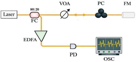
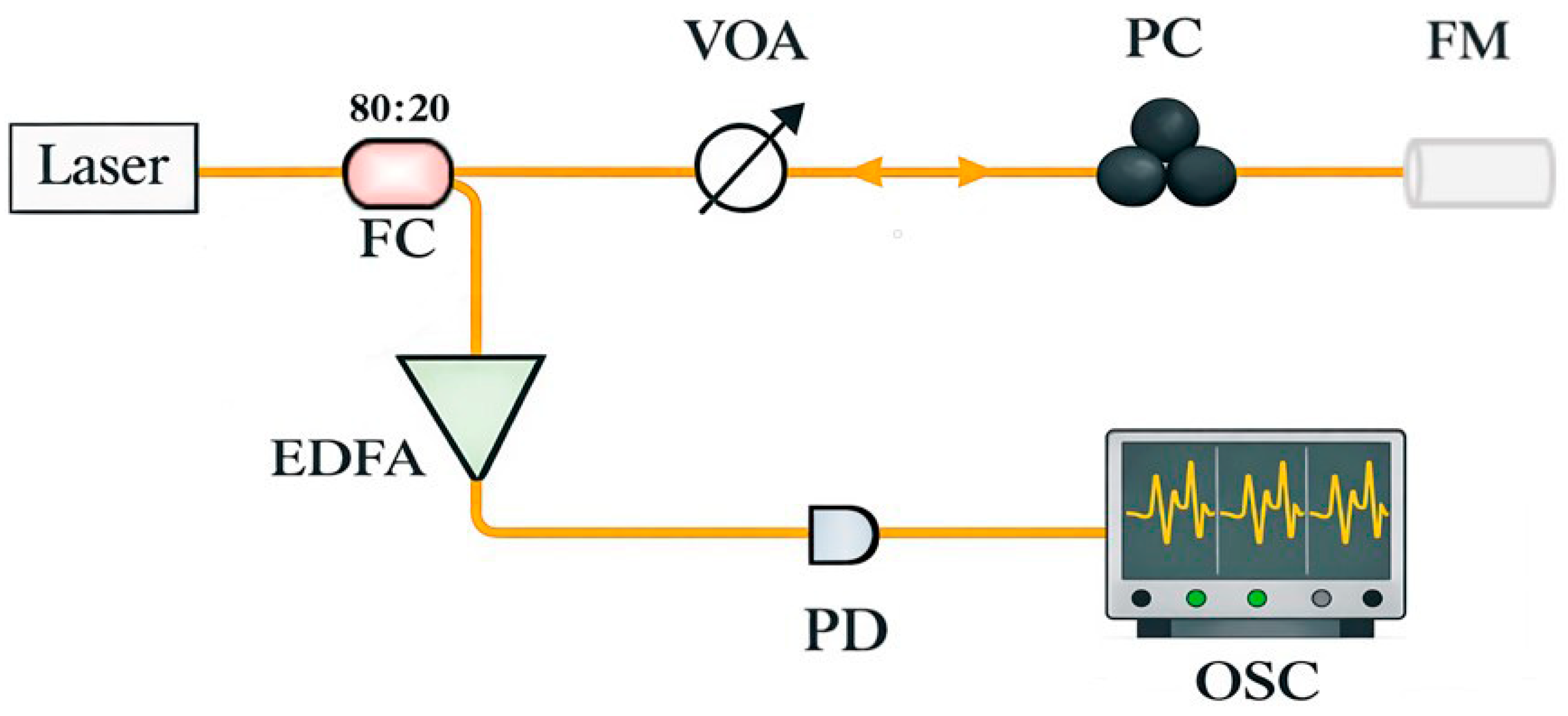
The schematic of the S-QPS signal generation experimental setup is shown in Figure 1. The bias current and temperature of the laser are controlled by a current source (LDX-3412, ILX Lightwave, Bozeman, MT, USA) and a temperature controller (LDT-5416, ILX Lightwave, Bozeman, MT, USA), respectively. The optical output of the semiconductor laser is split into two paths by an 80:20 fiber coupler (FC). One portion (80%) of the light is reflected by a fiber mirror (FM) and then fed back into the laser to induce nonlinear dynamical behavior. A polarization controller (PC) is used to match the polarization of the feedback light with the laser, and a variable optical attenuator (VOA) is used to adjust the feedback power. The feedback ratio κf is defined as the ratio of the feedback power to the laser output power. The external cavity length of the feedback loop is about 7.4 m, corresponding to an external cavity round-trip time of 74 ns. The other portion (20%) of the optical signal is amplified by an erbium-doped fiber amplifier (EDFA), converted into an electrical signal using a 50-GHz bandwidth photodetector (Finisar, XPDV2120RA, Sunnyvale, CA, USA), and recorded using a real-time oscilloscope (MSO73304DX, Tektronix, Beaverton, OR, USA) with a bandwidth of 33 GHz and a sampling rate of 100 GS/s.
Figure 1.
Experimental setup of the S-QPS signal generation. FC: fiber coupler; VOA: variable optical attenuator; PC: polarization controller; FM: fiber mirror; EDFA: erbium-doped fiber amplifier; PD: photodetector; OSC: oscilloscope.
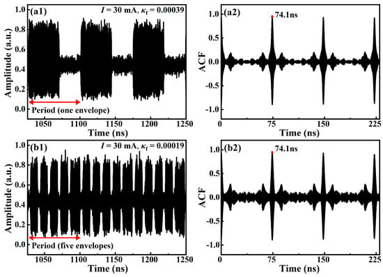
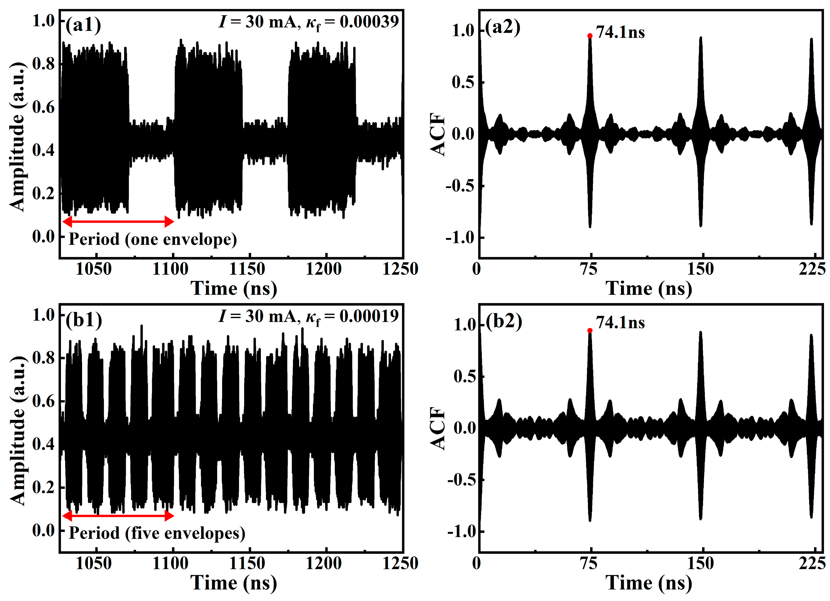
Figure 2 shows the obtained output time series of two typical S-QPS states and their corresponding autocorrelation functions at a bias current of I = 30 mA with feedback ratios of κf = 0.00039 and κf = 0.00019, respectively. The time series consist of high-frequency oscillations and low-frequency envelopes, revealing a clear multiscale temporal structure. It is clear that, combined with their autocorrelation functions, both signals exhibit a period of 74.1 ns, which corresponds to the external cavity round-trip time. The time series reveal that the first signal has one envelope per period (referred to as Exp. 1-envelope signal) and the second has five envelopes per period (referred to as Exp. 5-envelope signal), as shown in Figure 2(a1) and (b1), respectively. The property of the period combined with the external cavity length can meet the requirements of the different processing rates of the TDRC. Meanwhile, the significant amplitude fluctuations exhibited in their quasi-periodic segments show excellent numerical diversity, which satisfies the demand for realizing high-dimensional conversion. Thus, the S-QPS signal is a highly promising mask signal at first glance. To ensure consistency in the amplitude range when the signals are subsequently used as mask signals, all experimentally measured time series data are linearly normalized, with their amplitudes mapped into the interval [0, 1].
Figure 2.
The time series (a1,a2) and the corresponding autocorrelation function curves (b1,b2) of two typical S-QPS states, with the condition: bias current of I = 30 mA with feedback ratio of κf = 0.00039 (a1,a2) and κf = 0.00019 (b1,b2).
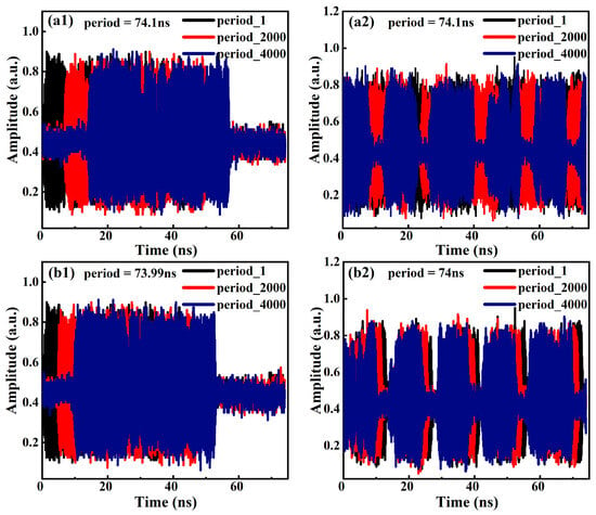
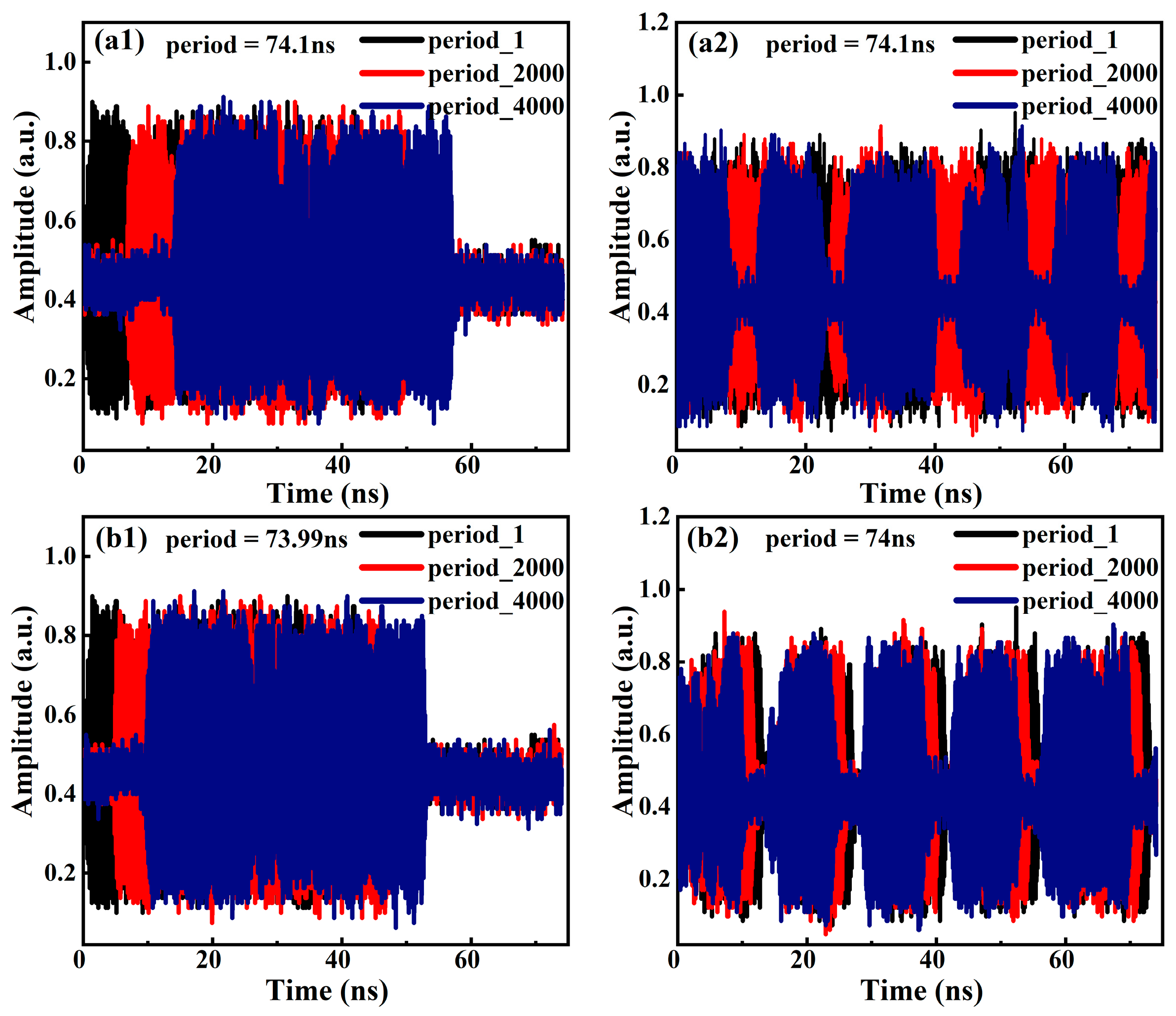
To better evaluate the applicability of S-QPS signals as mask signals, we investigated their long-term temporal characteristics in detail. Specifically, the 1st, 2000th, and 4000th periods of the Exp. 1-envelope and Exp. 5-envelope signals are extracted using the 74.1 ns period obtained from the autocorrelation function and overlaid, as shown in Figure 3(a1,a2). In total, 4000 periods are selected to match the number of periods used in the subsequent TDRC task. It can be clearly observed that, as the period number increases from 1 to 4000, the envelopes of both signals exhibit an obvious temporal offset, which is inconsistent with our expectations. This indicates that the time-domain repeatability of the signals is not optimal when 74.1 ns is used as the overlay period.
Figure 3.
Overlay of representative periods extracted from the experimental time series for the Exp. 1-envelope signal and Exp. 5-envelope signal. The 1st, 2000th, and 4000th periods are shown to compare long-term period consistency. (a1,a2) Period overlays using a period of 74.1 ns; (b1,b2) Period overlays using period of 73.99 ns (for Exp. 1-envelope signal) and 74.0 ns (for Exp. 5-envelope signal).
Therefore, we fine-tune the period length to more accurately determine the effective repetition period. The results show that, when the period of Exp. 1-envelope signal is set to 73.99 ns and that of Exp. 5-envelope signal to 74.0 ns, the overlap of the curves for different periods is significantly improved as shown in Figure 3(b1,b2). In the subsequent mask construction and TDRC analyses, the period T of the two S-QPS signals is taken as 73.99 ns and 74.0 ns, respectively.
Moreover, the period overlay curves of different period numbers do not overlap perfectly, manifesting in both the phase and amplitude factors. In terms of phase, as the period number increases, the period envelopes of both signals exhibit a gradual temporal offset. Moreover, this period offset accumulates over multiple periods. In terms of amplitude, noticeable amplitude fluctuations are also observed among different periods, indicating that the signal amplitude and local waveform details cannot be maintained identically from period to period. These phenomena are possibly caused by device noise and environmental disturbances.
2.2. Evaluation
A simulated opto-electronic TDRC system [34] with a Santa Fe time-series prediction task [35] test is employed to evaluate the suitability of these two signals as masks. To accommodate the task configuration of 3000 training steps and 1000 testing steps (totaling 4000 steps), we collected experimental time-series data at a sampling rate of 100 GS/s with a total duration of 370 μs, which far exceeds the required time length of 4000 × 74 ns = 296 μs and fully satisfies the data volume demand for both the training and testing.
We directly use 4000 consecutive periods extracted from the output time series of the Exp. 1-envelope signal and Exp. 5-envelope signal as masks applied to the TDRC system. The virtual node interval θ is treated as a tunable parameter, and the number of virtual nodes N is varied correspondingly based on θ. Since T/θ is generally not an integer, N is determined by taking the floor of this ratio. The normalized Santa Fe benchmark time series are temporally expanded to ensure that each scalar input value spans one complete mask period. Then, each value is multiplied point-by-point with the mask to generate a masked signal. This signal is sequentially injected into the single nonlinear node implemented by a Mach–Zehnder modulator with delayed feedback. The responses of the virtual nodes are collected and processed using linear regression to obtain the prediction output.
The prediction performance is quantitatively evaluated using the normalized mean square error (NMSE). In general, when NMSE ≤ 0.1, the TDRC system is considered capable of effectively performing the Santa Fe chaotic time-series prediction task, indicating good prediction performance [36].
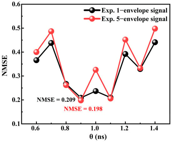
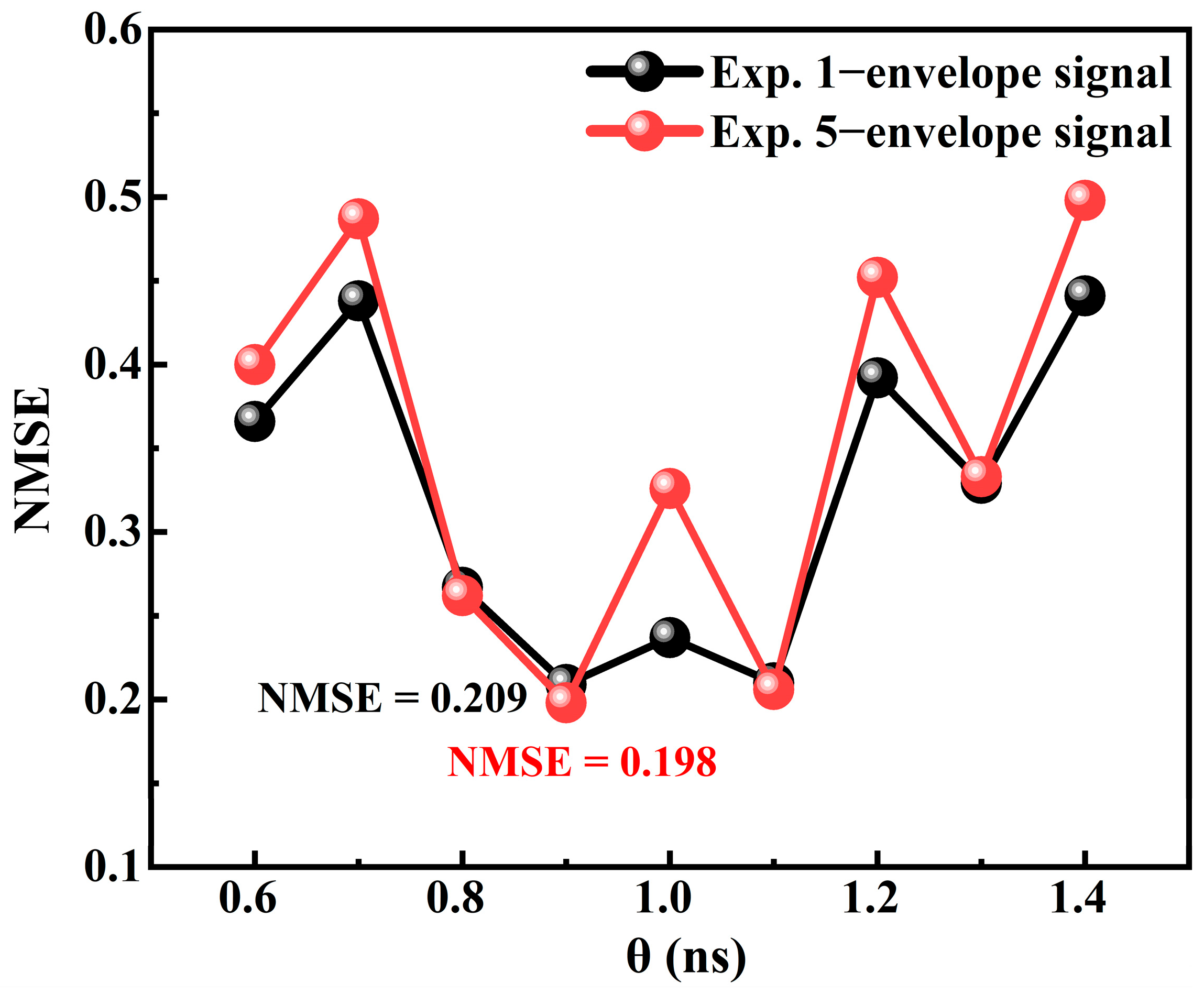
Figure 4 shows the NMSE using the two mask signals as a function of the virtual node interval θ from 0.6 ns to 1.4 ns. A large value of θ leads to an insufficient number of virtual nodes within a single period, thereby reducing the dimensionality of the reservoir state space and weakening its high-dimensional nonlinear mapping capability. Conversely, a small value of θ causes the transient responses of adjacent virtual nodes to be highly correlated, resulting in severe information redundancy that prevents the computing performance from being effectively improved. Overall, the scanning range of 0.6–1.4 ns corresponds to 53–123 virtual nodes per period, aligning well with the typical number of virtual nodes required for chaotic time-series prediction tasks in TDRC systems. From the perspective of hardware implementation constraints, the experiment employs a 100 GS/s oscilloscope with a sampling interval of 10 ps. The lower bound of the scanning range is set at 0.6 ns, which is much larger than this sampling interval. The black curves correspond to the NMSE results obtained using Exp. 1-envelope signal, while the red curves represent those using Exp. 5-envelope signal.
Figure 4.
NMSE as a function of the virtual node interval θ (ranging from 0.6 ns to 1.4 ns) using the two mask signals (Exp. 1-envelope signal and Exp. 5-envelope signal).
Across the entire scanned range of θ, similar NMSE trends are observed for the TDRC system using the two mask signals, where the NMSE first decreases and then increases as θ rises. This indicates that the proposed mask signals can, to some extent, support nonlinear dimensionality expansion in the TDRC system. However, the minimum NMSE values of the TDRC system using the two mask signals at θ = 0.9 ns are 0.209 and 0.198, respectively, which are higher than the standard threshold of 0.1. This performance is likely limited by experimental noise, such as that introduced by the laser, photodetector, amplifier, and oscilloscope.
The experimentally obtained S-QPS signals exhibit clear periodic structures and intra-period amplitude modulation at a macroscopic level, thereby formally satisfying the basic requirements of mask signal in TDRC. However, the actual prediction performance achieved remains unsatisfactory, likely affected by noise. Specifically, it can be attributed to two factors: period offset and amplitude fluctuations. In addition, these two factors are highly coupled in experiments, making it difficult to isolate their respective contributions solely through experimental means, and it remains unclear whether the period offset originates from the intrinsic dynamical characteristics of the system or from cumulative drift induced by noise. Therefore, in the subsequent study, we simulate the dynamic characteristics of an SL-OF using the Lang–Kobayashi rate equations to generate S-QPS signals under noise-free conditions. By testing their performance for TDRC and analyzing the effects of both phase and amplitude factors on system performance, the applicability of S-QPS signals as masks in TDRC is evaluated, providing theoretical support for their generation and practical application.
3. Simulation
The SL-OF system for generating S-QPS signals is simulated using the Lang–Kobayashi equations [37]:
A(t) denotes the amplitude of the optical field emitted by the laser, and N(t) represents the carrier density in the laser cavity. The feedback strength ξf is defined as (1 − r02)re/r0, with r0 and re being the amplitude reflectivities of the laser facet and the external mirror, respectively. τf refers to the external cavity round-trip time, and I is the bias current. The optical phase is expressed as φ(t), and the optical feedback phase difference is defined as θdiff = ω0τf + φ(t) − φ(t − τf). The second terms on the right-hand sides of Equations (1) and (2) correspond to the feedback terms, describing the amplitude and phase variation rates induced by optical feedback. The rate equations are solved using a fourth-order Runge–Kutta method, and the main laser parameters and their values are listed in Table 1.
Table 1.
Values of the parameters for SL-OF.
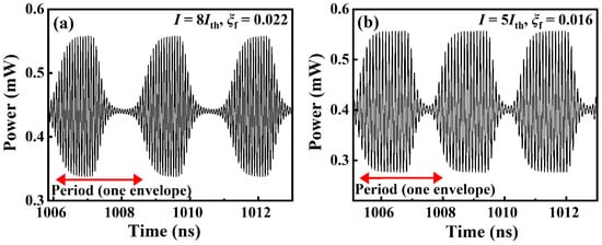
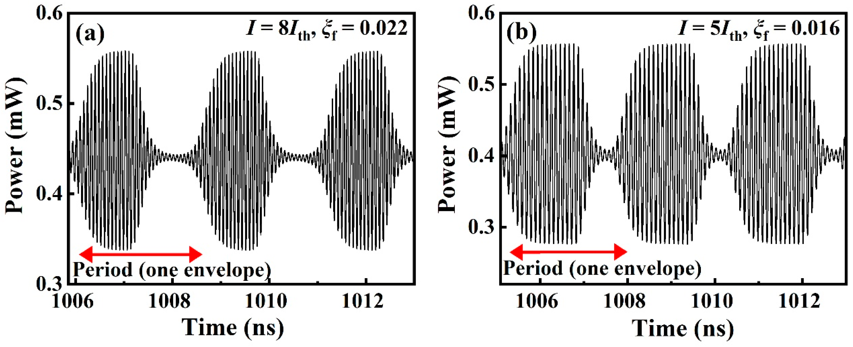
Figure 5 shows two S-QPS signals with different shapes from laser output under noise-free conditions with an external-cavity round-trip time of τf = 2.5 ns. When the bias current is set to I = 8Ith and the feedback strength is ξf = 0.022, the signal (referred to as the Sim. Long steady-state signal) exhibits a typical S-QPS state, as shown in Figure 5a. Compared with the experimentally observed signals, the envelope modulation is more regular, and the inter-period waveform repeatability is significantly improved. This output features a periodic structure composed of one envelope per period, the period of which is 2.608 ns, matching closely with τf. A similar signal (referred to as Sim. Short steady-state signal) is obtained for I = 5Ith and ξf = 0.016, with a period of 2.644 ns. Compared with Figure 5a, the duration of the steady state is shortened and the two signals exhibit slightly different periods.
Figure 5.
S-QPS states of an SL-OF under noise-free conditions with an external-cavity round-trip time of τf = 2.5 ns: (a,b) simulated time series at I = 8Ith, ξf = 0.022 and I = 5Ith, ξf = 0.016, respectively.
As described above, the long-time-scale period evolution analysis is carried out on the two simulated signals in Figure 5 to identify the source of the observed period offset. By selecting and comparing representative periods at different instants, we examine the temporal consistency of the period structure and its evolution over time. Note that numerical simulations are implemented with a fixed discretization time step (0.002 ns in this work). Consequently, certain simulated periods (e.g., 2.61 ns and 2.646 ns) deviate from the corresponding reference periods (2.608 ns and 2.644 ns) by one sampling interval, which may impede the accurate analysis of period consistency and temporal evolution. Therefore, these periods are excluded, and only those exactly matching the reference periods are retained. This eliminates numerical deviations introduced by discrete-time sampling, ensuring the reliability of period evolution analysis.
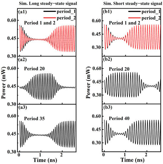
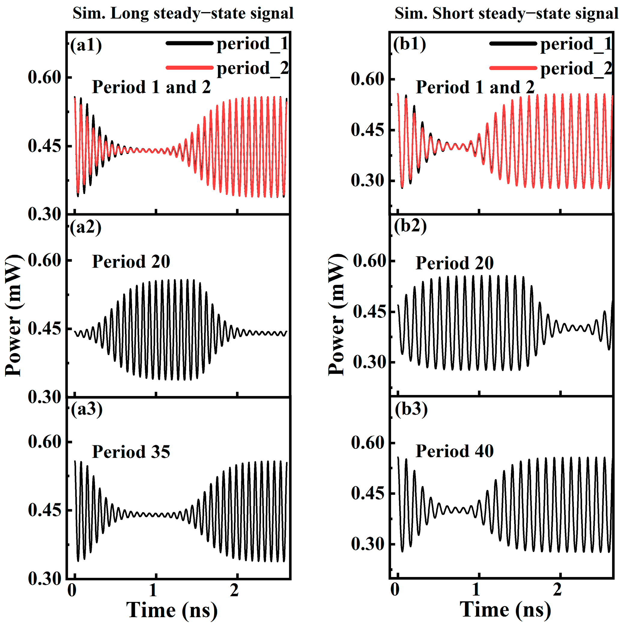
Figure 6 shows the magnified time series of the selected periods. Figure 6(a1–a3,b1–b3) corresponds to the Sim. Long steady-state signal and the Sim. Short steady-state signal, respectively. As seen in Figure 6(a1,b1), the time series of the first and second periods nearly overlap, confirming high temporal consistency between consecutive periods. By comparing the 1st, 20th, and 35th periods in Figure 6(a1–a3), as well as the 1st, 20th, and 40th periods in Figure 6(b1–b3), we observe that the envelope gradually shifts along the time axis with increasing period number and then returns to near its initial position after 35 and 40 periods, respectively, exhibiting a clear “offset–return” behavior.
Figure 6.
Time series of two noise-free simulated S-QPS signals for different periods: (a1) overlay of the first and second periods, (a2,a3) the 20th and 35th periods of Sim. Long steady-state signal; (b1) overlay of the first and second periods, (b2,b3) the 20th and 40th periods of Sim. Short steady-state signal.
These results demonstrate that period offset persists in the S-QPS signals even in the complete absence of noise. This behavior indicates that the observed period offset is not noise-induced but rather an intrinsic property of the S-QPS states.
We construct mask signals using the identical procedure employed in the experiments and perform the Santa Fe time-series prediction task. The signal period is set to T = 2.608 ns for the Sim. Long steady-state signal and T = 2.644 ns for the Sim. Short steady-state signal. To investigate the influence of period offset on prediction performance, two types of mask signals are prepared for comparison. The first type retains the natural period offset behavior (referred to as Offset mask). For comparison, an ideal mask without period offset (referred to as Non-offset mask) is constructed by extracting a single reference period from the same signal and repeating it exactly 4000 times. This ensures perfect alignment among all periods with no temporal misalignment.
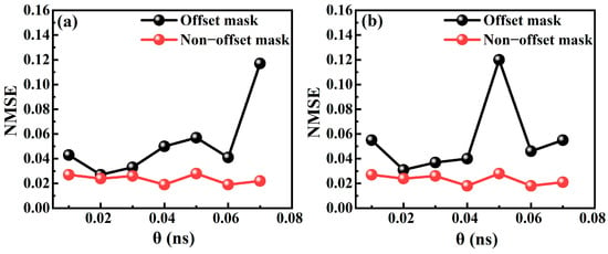
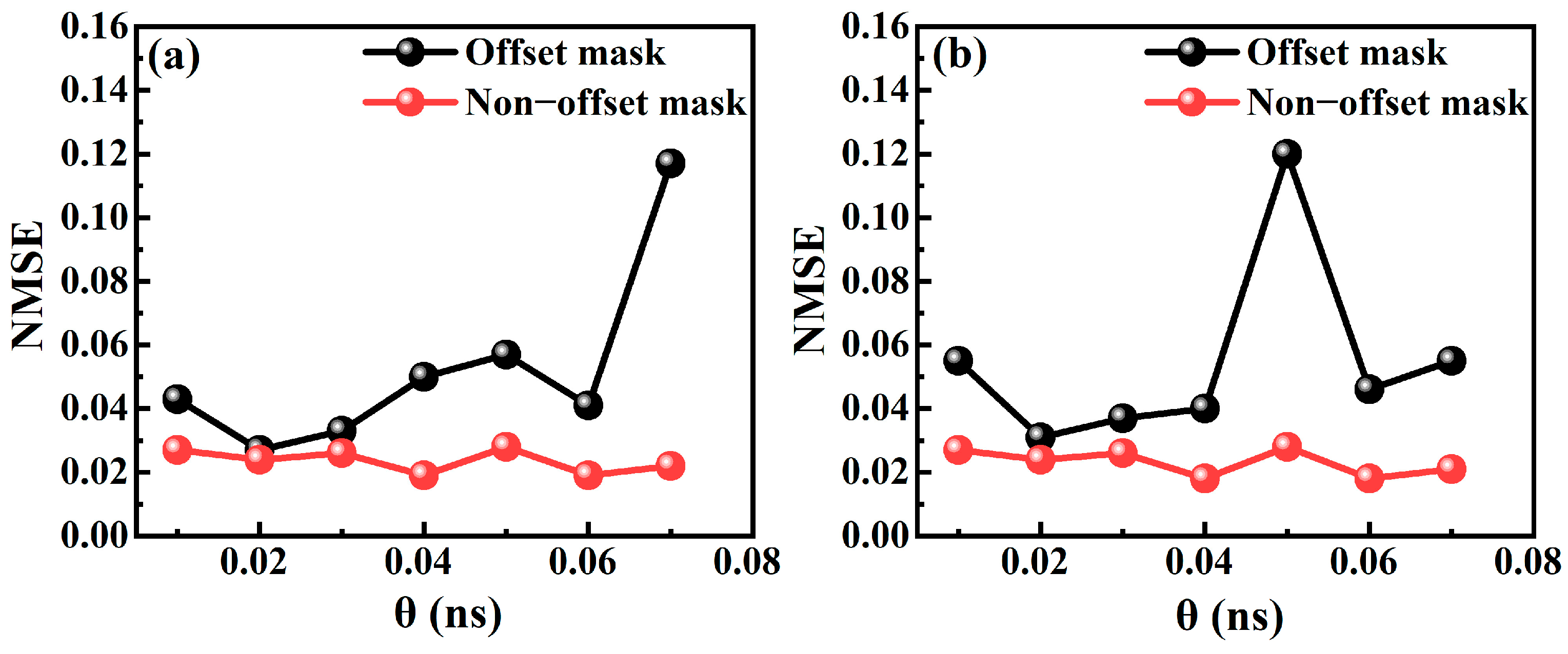
Figure 7 presents the NMSE obtained using the two mask signals as a function of the virtual node interval θ from 0.01 ns to 0.07 ns, with (a) and (b) corresponding to the Sim. Long steady-state signal and the Sim. Short steady-state signal, respectively. The black curves correspond to the NMSE results obtained with the Offset masks, while the red curves represent those with the Non-offset masks. Overall, for both mask signals, the use of Non-offset masks consistently yields lower NMSE values over the entire scanned range of θ. In Figure 7a, the NMSE obtained with the Offset mask remains stable at 0.02–0.05 in the low θ range (θ ≤ 0.04 ns) and then gradually rises to 0.11 as θ increases to 0.07 ns. The system with the Non-offset mask maintains a low and stable NMSE of 0.019–0.028 across the entire θ range. In Figure 7b, the system with the Offset mask exhibits a distinct NMSE peak of 0.12 at θ = 0.05 ns, while the system with the Non-offset masks maintains a low NMSE, showing similar performance to that obtained with the Sim. Long steady-state signal. Combining the results of Figure 7a,b, under optimal θ conditions, the system with the Non-offset masks achieves a slightly lower NMSE than that with the Offset masks.
Figure 7.
NMSE comparison using masks with and without period offset as a function of the virtual node interval θ (ranging from 0.01 ns to 0.07 ns), (a,b) constructed from Sim. Long steady-state signal and Sim. Short steady-state signal. The black curves correspond to mask signals containing period offset, while the red curves correspond to ideal mask signals without period offset.
These results indicate that the tiny period offset, as an intrinsic dynamical feature, exerts a limited influence on reservoir computing performance. Although this offset disrupts the strict alignment between successive periods over finite durations, it exhibits an offset–return behavior over long time scales, which thus mitigates its adverse effects to a certain extent.
Furthermore, the performance degradation of the Offset mask becomes more pronounced as θ increases. We speculate that this behavior arises for the following reasons. When θ is small, each virtual node corresponds to a relatively short time segment. In this case, even if a slight period offset exists between adjacent cycles, the virtual nodes are likely to sample similar system responses. Therefore, the influence of the offset on the reservoir states remains limited. By contrast, as θ increases, each virtual node spans a longer temporal interval. In this condition, even a small period offset may cause the virtual nodes to sample noticeably different system responses, thereby increasing the inconsistency of the reservoir states across periods and leading to a larger performance gap compared with the non-offset mask. Based on this mechanism, selecting a smaller θ value can effectively mitigate the adverse effects of period offset, allowing offset masks to achieve near-optimal prediction performance in practical applications.
Following the phase analysis above, we further analyze the impact of the amplitude fluctuations induced by noise on TDRC performance, as well as the output response consistency of the system by directly superimposing Gaussian white noise on the two Non-offset mask signals. The virtual node interval θ is fixed at 0.04 ns, which corresponds to the value at which the system achieves optimal prediction performance, and the Santa Fe time-series prediction task is performed under this condition. By adjusting the noise amplitude, the impact of noise perturbations on the TDRC performance and the consistency of system outputs is systematically investigated. The noise strength is characterized by the signal-to-noise ratio (SNR), with its expression provided as follows:
where Psignal and Pnoise denote the average power of the mask signal and the Gaussian white noise, respectively. These power values are calculated as the average of the squared amplitudes over all signal points. A lower SNR corresponds to a higher noise level.
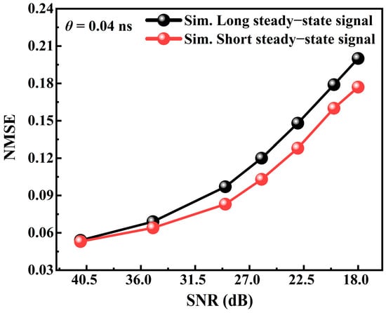
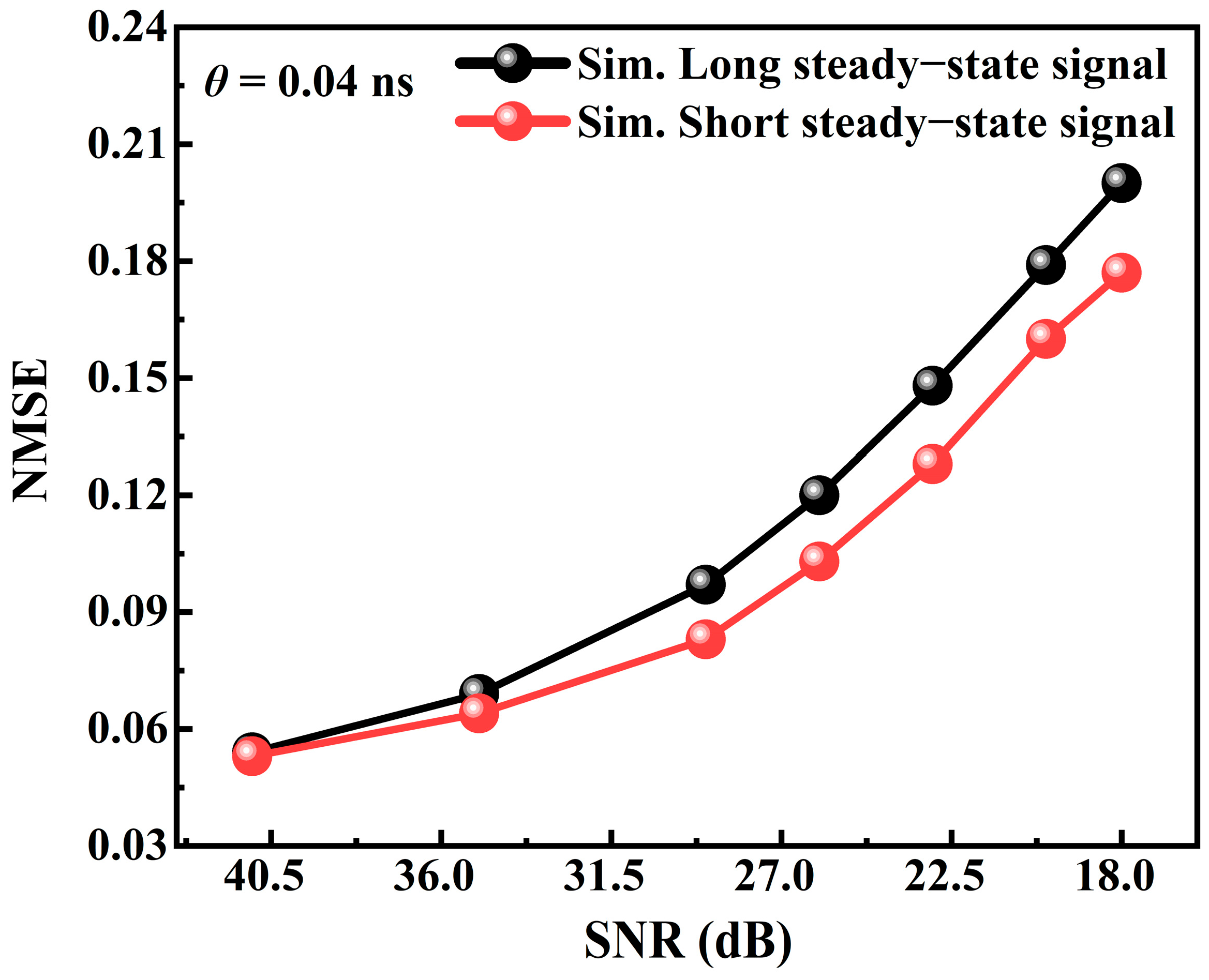
Figure 8 presents the variation in the NMSE using the two Non-offset mask signals under different SNR conditions. The black and red lines denote the results obtained with the Sim. Long steady-state signal and the Sim. Short steady-state signal, respectively. As the SNR decreases from 41 dB to 18 dB, the NMSE in both cases exhibits a clear monotonic increasing trend, indicating that increasing noise continuously degrades the prediction performance of the TDRC. In the high-SNR regime (41–29 dB), the system maintains relatively low prediction errors with both mask signals. However, when the SNR is reduced to 26 dB and below, the NMSE increases more rapidly, and the prediction performance deteriorates noticeably. These results demonstrate that the noise progressively degrades TDRC performance by disturbing the stability of the mask signals, with a pronounced performance deterioration occurring at low SNR levels. By comparison, under the same SNR conditions, the NMSE obtained with the Sim. Long steady-state signal is consistently slightly higher than that of the Sim. Short steady-state signal, indicating relatively weak noise robustness. This difference may be attributed to the disparity in steady-state duration: the steady-state process is more susceptible to noise, and this effect tends to accumulate over longer durations.
Figure 8.
NMSE as a function of the SNR (ranging from 41 dB to 18 dB) for the Santa Fe time-series prediction task with θ = 0.04 ns, where additive Gaussian white noise of varying amplitude is injected into the two mask signals. The black curves correspond to Sim. Long steady-state signal, while the red curves correspond to Sim. Short steady-state signal.
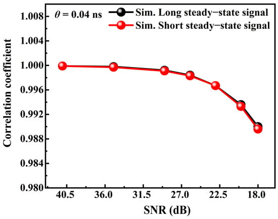
On this basis, we further evaluate the system response consistency under different noise levels. For each tested SNR level, we fix the original mask waveform and average noise power level and superimpose two independent random noise sequences onto the mask signal to conduct two groups of repeated simulations. The response consistency at the same noise power is evaluated by calculating the Pearson correlation coefficient between the two output responses obtained from the two runs. To further ensure reliability, we repeat this process five times for each SNR level and take the average of the resulting correlation coefficients.
As shown in Figure 9, the correlation coefficient exhibits a slight downward trend as the SNR decreases. For both the Sim. Long and Sim. Short steady-state signals, the correlation coefficients remain above 0.988 and the two curves nearly overlap across the entire tested SNR range from 41 dB down to 18 dB. Even under low SNR, the correlation coefficient only drops marginally. This result demonstrates that response consistency is only slightly weakened by noise-induced amplitude fluctuations.
Figure 9.
Correlation coefficient as a function of the SNR (ranging from 41 dB to 18 dB) for the Santa Fe time-series prediction task with θ = 0.04 ns, where additive Gaussian white noise of varying amplitude is injected into the two mask signals. The black curves correspond to the Sim. Long steady-state signal, while the red curves correspond to the Sim. Short steady-state signal.
In summary, Period offset and noise affect TDRC performance in two distinct dimensions with vastly different impacts. The adverse impact of period offset is mitigated by the inherent offset–return behavior. The amplitude fluctuations induced by noise exert a dominant influence, causing irreversible and cumulative fluctuations in mask signals.
4. Discussion
Both experimental and numerical results demonstrate that S-QPS signals satisfy the fundamental requirements for TDRC mask signals. The signal period can be flexibly tuned through the external cavity length to match different processing rates, while the rich intra-period amplitude modulation provides sufficient numerical diversity for high-dimensional nonlinear mapping. The experimentally obtained S-QPS masks exhibit limited prediction performance in the Santa Fe time-series prediction task, mainly due to the noise introduced in the experimental devices. Noise-free simulations confirm that period offset is an intrinsic dynamical property of S-QPS signals. Its influence on reservoir performance is limited and can be effectively mitigated by selecting an appropriate virtual node interval. In contrast, amplitude noise is identified as the dominant factor degrading reservoir performance. It introduces random fluctuations in signal amplitude and local waveform structures, leading to the irreversible deterioration of reservoir-state consistency and a significant reduction in prediction accuracy as the noise level increases.
Therefore, future research should prioritize suppressing this dominant amplitude noise to bridge the gap between experiment and simulation.
5. Conclusions
This study systematically investigates the feasibility of using S-QPS signals generated by SL-OF as mask signals for TDRC. By combining experimental measurements and numerical simulations, the long-term dynamical characteristics of S-QPS signals (including period consistency, period offset, and noise-induced perturbations) are analyzed, and their impacts on TDRC prediction performance are quantitatively evaluated.
These results verify the potential of S-QPS signals as optical masks for TDRC and clarify the distinct roles of period offset and noise in affecting system performance. This study lays a foundation for the generation, optimization, and practical application of this type of mask signal.
Future research can be carried out on the following three areas. First, regarding signal generation, reinforcement learning [38,39,40,41] will be introduced to optimize the laser bias current and feedback strength for the adaptive generation of optimal S-QPS mask signals. Meanwhile, the Riemann–Hilbert approach and Lie-group numerical methods will be employed to analyze the optical feedback laser dynamics, enabling the precise regulation of the mask period and envelope shape [42,43].
Second, a noticeable performance gap exists between the experimental and simulation results, which is primarily caused by noise. To address this issue, noise suppression efforts will proceed at both experimental and algorithmic levels. Experimentally, we have completed noise calibration tests for the key devices in the optical path. The results show that the EDFA and the photodetector introduce noise figures of approximately 3.8 dB and 4.5 dB, respectively, while the oscilloscope exhibits a background noise floor of approximately 0.8 mV RMS. In addition, optical path reflections also introduce a certain level of noise into the system. On this basis, research will focus on optical link optimization, such as by inserting optical filters and implementing strict temperature control of the devices. Algorithmically, PDE-based image denoising algorithms will be utilized to preprocess the collected optical time-series data [44], thereby weakening the interference of experimental noise. Additionally, an improved PINN framework will be adopted to construct a hybrid TDRC system, improving the time-series prediction accuracy under strong noise conditions [45,46].
Third, to verify the general applicability of the proposed scheme, the research will be expanded in two dimensions. On the one hand, the S-QPS mask scheme will be applied to more complex reservoir computing tasks, including image recognition and multi-step prediction. On the other hand, the mask scheme will be adapted to quasi-convolution coding-based reservoir computing frameworks [47], to further evaluate its cross-architecture performance and application potential.
Author Contributions
Conceptualization, T.Z. and T.C.; methodology, T.Z.; software, T.Z. and T.C.; validation, T.C., B.F. and Z.B.; formal analysis, T.Z.; investigation, T.C.; resources, X.F.; data curation, T.C. and B.F.; writing—original draft preparation, T.Z.; writing—review and editing, T.Z., T.C., B.F. and Z.B.; visualization, P.C. and L.Q.; supervision, X.F.; project administration, T.Z.; funding acquisition, S.Y. and X.F. All authors have read and agreed to the published version of the manuscript.
Funding
This research was supported by the National Natural Science Foundation of China (No. U23A20375), the National Natural Science Foundation of China (Nos. 52273252 and 62475185), the Development Fund in Science and Technology of Shanxi Province (No. YDZJSX2024D018), and the Shanxi Provincial Key Research and Development Project (Nos. 202202030201004 and 202302150101002).
Data Availability Statement
The data that support the findings of this study are available from the corresponding author upon reasonable request.
Conflicts of Interest
Author Su Yan was employed by the company Fenyang Fengyuan Grid Co., Ltd. The remaining authors declare that the research was conducted in the absence of any commercial or financial relationships that could be construed as a potential conflict of interest.
References
- Lukoševičius, M.; Jaeger, H. Reservoir computing approaches to recurrent neural network training. Comput. Sci. Rev. 2009, 3, 127–149. [Google Scholar] [CrossRef] [Scilit]
- Tanaka, G.; Yamane, T.; Héroux, J.B.; Nakane, R.; Kanazawa, N.; Takeda, S.; Numata, H.; Nakano, D.; Hirose, A. Recent advances in physical reservoir computing: A review. Neural Netw. 2019, 115, 100–123. [Google Scholar] [CrossRef] [Scilit] [PubMed]
- Abdalla, M.; Van der Sande, G.; Argyris, A.; Pavanello, F.; Soriano, M.C.; Rontani, D. Photonic reservoir computing: A thematic review. J. Phys. Photonics 2026, 8, 022003. [Google Scholar]
- Li, X.Z.; Sheng, B.; Zhang, M. Predicting the dynamical behaviors for chaotic semiconductor lasers by reservoir computing. Opt. Lett. 2022, 47, 2822–2825. [Google Scholar] [CrossRef] [Scilit] [PubMed]
- Abreu, F.A.; Riou, M.; Torrejon, J.; Bolea, A.; Tsunegi, S.; Querlioz, D.; Yakushiji, K.; Fukushima, A.; Kubota, H.; Yuasa, S.; et al. Role of non-linear data processing on speech recognition task in the framework of reservoir computing. Sci. Rep. 2020, 10, 328. [Google Scholar] [CrossRef] [Scilit]
- Qu, Y.; Lian, H.; Shao, R.; Liu, J.; Liu, L.; Yang, J. Time series analysis for financial indices using optical reservoir computing. Opt. Eng. 2024, 63, 054108. [Google Scholar] [CrossRef] [Scilit]
- Appeltant, L.; Soriano, M.C.; Sande, G.V.; Danckaert, J.; Massar, S.; Dambre, J.; Schrauwen, B.; Mirasso, C.R.; Fischer, I. Information processing using a single dynamical node as complex system. Nat. Commun. 2011, 2, 468. [Google Scholar] [CrossRef] [Scilit] [PubMed]
- Xu, J.W.; Zhao, T.; Chang, P.F.; Wang, C.; Wang, A.B. Photonic reservoir computing with a silica microsphere cavity. Opt. Lett. 2023, 48, 3653–3656. [Google Scholar] [CrossRef] [Scilit] [PubMed]
- Zhou, H.X.; Xiang, S.Y.; Guo, X.X.; Gu, B.L.; Yu, Q.; Hao, Y. Photonic convolutional reservoir computing based on VCSEL with multiple optical injections. Opt. Commun. 2023, 545, 129711. [Google Scholar] [CrossRef] [Scilit]
- Takano, K.; Sugano, C.; Inubushi, M.; Yoshimura, K.; Sunada, S.; Kanno, K.; Uchida, A. Compact reservoir computing with a photonic integrated circuit. Opt. Express 2018, 26, 29424–29439. [Google Scholar] [CrossRef] [Scilit] [PubMed]
- Harkhoe, K.; Verschaffelt, G.; Katumba, A.; Bienstman, P.; Van der Sande, G. Demonstrating delay-based reservoir computing using a compact photonic integrated chip. Opt. Express 2020, 28, 3086–3096. [Google Scholar] [CrossRef] [Scilit] [PubMed]
- Sugano, C.; Kanno, K.; Uchida, A. Reservoir computing using multiple lasers with feedback on a photonic integrated circuit. IEEE J. Sel. Top. Quantum Electron. 2019, 26, 1–9. [Google Scholar] [CrossRef] [Scilit]
- Donati, G.; Argyris, A.; Mancinelli, M.; Mirasso, C.R.; Pavesi, L. Time delay reservoir computing with a silicon microring resonator and a fiber-based optical feedback loop. Opt. Express 2024, 32, 13419–13437. [Google Scholar] [CrossRef] [Scilit] [PubMed]
- Ren, H.L.; Li, Y.J.; Li, M.; Gao, M.Y.; Lu, J.; Zou, C.L.; Dong, C.H.; Yu, P.Q.; Yang, X.N.; Xuan, Q. Photonic time-delayed reservoir computing based on series-coupled microring resonators with high memory capacity. Opt. Express 2024, 32, 11202–11220. [Google Scholar] [PubMed]
- Zhang, J.F.; Ma, B.W.; Zou, W.W. High-speed parallel processing with photonic feedforward reservoir computing. Opt. Express 2023, 31, 43920–43933. [Google Scholar] [CrossRef] [Scilit] [PubMed]
- Picco, E.; Jaurigue, L.; Lüdge, K.; Massar, S. Efficient optimisation of physical reservoir computers using only a delayed input. Commun. Eng. 2025, 4, 3. [Google Scholar] [CrossRef] [Scilit] [PubMed]
- Kuriki, Y.; Nakayama, J.; Takano, K.; Uchida, A. Impact of input mask signals on delay-based photonic reservoir computing with semiconductor lasers. Opt. Express 2018, 26, 5777–5788. [Google Scholar] [CrossRef] [Scilit] [PubMed]
- Appeltant, L.; Van der Sande, G.; Danckaert, J.; Fischer, I. Constructing optimized binary masks for reservoir computing with delay systems. Sci. Rep. 2014, 4, 3629. [Google Scholar] [CrossRef] [Scilit] [PubMed]
- Soriano, M.C.; Ortin, S.; Brunner, D.; Larger, L.; Mirasso, C.R.; Fischer, I.; Pesquera, L. Optoelectronic reservoir computing: Tackling noise-induced performance degradation. Opt. Express 2013, 21, 12–20. [Google Scholar] [CrossRef] [Scilit] [PubMed]
- Nakayama, J.; Kanno, K.; Uchida, A. Laser dynamical reservoir computing with consistency: An approach of a chaos mask signal. Opt. Express 2016, 24, 8679–8692. [Google Scholar] [CrossRef] [Scilit] [PubMed]
- Duport, F.; Smerieri, A.; Akrout, A.; Haelterman, M.; Massar, S. Fully analogue photonic reservoir computer. Sci. Rep. 2016, 6, 22381. [Google Scholar] [CrossRef] [Scilit] [PubMed]
- Argyris, A.; Schwind, J.; Fischer, I. Fast physical repetitive patterns generation for masking in time-delay reservoir computing. Sci. Rep. 2021, 11, 6701. [Google Scholar] [CrossRef] [Scilit] [PubMed]
- Yue, Y.L.; Liu, S.J.; Zhai, Y.R.; Wang, C. Enhanced photonic time-stretch reservoir computing using all-optical input masks. In Proceedings of the 2022 IEEE Photonics Conference (IPC), Vancouver, BC, Canada, 13–17 November 2022; pp. 1–2. [Google Scholar]
- Yue, Y.L.; Liu, S.J.; Wang, C. Photonic Time Stretch Reservoir Computer Using a Multi-mode Fibre-based Optical Mask. In Proceedings of the 2024 IEEE Photonics Conference (IPC), Rome, Italy, 10–14 November 2024; pp. 1–2. [Google Scholar]
- Chen, J.H.; Hou, Y.S.; Guo, X.Y.; Li, Q.D.; Li, S.Y.; Guo, C.L.; Yue, D.Z. Real-time masking in photonic reservoir computing based on semiconductor lasers. Appl. Phys. B 2025, 131, 149. [Google Scholar] [CrossRef] [Scilit]
- Bauwens, I.; Bienstman, P.; Verschaffelt, G.; Van der Sande, G. Use of a simple passive hardware mask to replace the digital masking procedure in photonic delay-based reservoir computing. IEEE J. Sel. Top. Quantum Electron. 2024, 31, 1–12. [Google Scholar] [CrossRef] [Scilit]
- Wu, X.N.; Lin, Z.S.; Deng, J.L.; Li, J.; Feng, Y. Nonmasking-based reservoir computing with a single dynamic memristor for image recognition. Nonlinear Dyn. 2024, 112, 6663–6678. [Google Scholar] [CrossRef] [Scilit]
- Abdalla, M.; Cardoso, R.; Jimenez, P.; de Queiroz, M.G.; Boes, A.; Ren, G.H.; Mitchell, A.; O’Connor, I.; Pavanello, F. Mask-less asynchronous time-delay reservoir computing using a passive photonic integrated circuit. J. Light. Technol. 2024, 42, 8051–8060. [Google Scholar] [CrossRef] [Scilit]
- Dong, J.X.; Zhuang, J.P.; Chan, S.C. Tunable switching between stable and periodic states in a semiconductor laser with feedback. Opt. Lett. 2017, 42, 4291–4294. [Google Scholar] [CrossRef] [Scilit] [PubMed]
- Dong, J.X.; Ruan, J.; Zhang, L.; Chen, H.W. Stable-unstable switching dynamics in semiconductor lasers with external cavities. Phys. Rev. A 2021, 103, 053524. [Google Scholar] [CrossRef] [Scilit]
- Zhang, T.; Jia, Z.W.; Wang, A.B.; Hong, Y.H.; Wang, L.S.; Guo, Y.Y.; Wang, Y.C. Experimental observation of dynamic-state switching in VCSELs with optical feedback. IEEE Photon. Technol. Lett. 2021, 33, 335–338. [Google Scholar] [CrossRef] [Scilit]
- Wang, T.; Tu, Z.C.; Ma, Y.X.; Li, Y.H.; Li, Z.B.; Qin, F.; Barland, S.; Xiang, S.Y. Fast square-oscillations in semiconductor VCSELs with delayed orthogonal polarization feedback. Opt. Express 2025, 33, 18601–18610. [Google Scholar] [CrossRef] [Scilit] [PubMed]
- Zhong, Z.Q.; Chang, D.; Jin, W.; Lee, M.W.; Wang, A.B.; Jiang, S.; He, J.X.; Tang, J.M.; Hong, Y.H. Intermittent dynamical state switching in discrete-mode semiconductor lasers subject to optical feedback. Photonics Res. 2021, 9, 1336–1342. [Google Scholar] [CrossRef] [Scilit]
- Larger, L.; Soriano, M.C.; Brunner, D.; Appeltant, L.; Gutierrez, J.M.; Pesquera, L.; Mirasso, C.R.; Fischer, I. Photonic information processing beyond Turing: An optoelectronic implementation of reservoir computing. Opt. Express 2012, 20, 3241–3249. [Google Scholar] [CrossRef] [Scilit] [PubMed]
- Weigend, A.S. Time Series Prediction: Forecasting the Future and Understanding the Past; Routledge: London, UK, 2018. [Google Scholar]
- Nguimdo, R.M.; Verschaffelt, G.; Danckaert, J.; Van der Sande, G. Fast photonic information processing using semiconductor lasers with delayed optical feedback: Role of phase dynamics. Opt. Express 2014, 22, 8672–8686. [Google Scholar] [CrossRef] [Scilit] [PubMed]
- Lang, R.; Kobayashi, K. External optical feedback effects on semiconductor injection laser properties. IEEE J. Quantum Electron. 1980, 16, 347–355. [Google Scholar] [CrossRef] [Scilit]
- Qiu, W.X.; Geng, K.L.; Zhu, B.W.; Liu, W.; Li, J.T.; Dai, C.Q. Data-driven forward-inverse problems of the 2-coupled mixed derivative nonlinear Schrödinger equation using deep learning. Nonlinear Dyn. 2024, 112, 10215–10228. [Google Scholar] [CrossRef] [Scilit]
- Zhou, T.H.; Zhao, R.M.; Yu, Z.X.; Yan, X.; Li, J.T.; Dai, C.Q. Predicting PT-symmetric solitons in competing cubic–quintic saturable medium via enhanced PINN with quadratic residual and reinforcement learning-based sampling. Opt. Laser Technol. 2026, 198, 114887. [Google Scholar] [CrossRef] [Scilit]
- Zhang, H.W.; Zhang, R.F.; Liu, Q.R. A novel multi-modal neurosymbolic reasoning intelligent algorithm for BLMP equation. Chin. Phys. Lett. 2025, 42, 100002. [Google Scholar] [CrossRef] [Scilit]
- Zhao, Z.L.; Zhang, R.F. Artificial Intelligence-Enhanced Mathematical Derivation method: Exact solutions of the Benjamin–Bona–Mahony equation. Eng. Appl. Artif. Intell. 2026, 173, 114464. [Google Scholar] [CrossRef] [Scilit]
- Wei, H.Y.; Fan, E.G.; Guo, H.D. Riemann–Hilbert approach and nonlinear dynamics of the coupled higher-order nonlinear Schrödinger equation in the birefringent or two-mode fiber. Nonlinear Dyn. 2021, 104, 649–660. [Google Scholar]
- Yin, F.L.; Xu, Z.Z.; Fu, Y.Y. Novel high-order explicit energy-preserving schemes for NLS-type equations based on the Lie-group method. Math. Comput. Simul. 2024, 225, 570–585. [Google Scholar] [CrossRef] [Scilit]
- Tian, C.; Chen, Y. Image segmentation and denoising algorithm based on partial differential equations. IEEE Sens. J. 2019, 20, 11935–11942. [Google Scholar] [CrossRef] [Scilit]
- Qiu, W.X.; Si, Z.Z.; Mou, D.S.; Dai, C.Q.; Li, J.T.; Liu, W. Data-driven vector degenerate and nondegenerate solitons of coupled nonlocal nonlinear Schrödinger equation via improved PINN algorithm. Nonlinear Dyn. 2025, 113, 4063–4076. [Google Scholar]
- Zhao, R.M.; Qiu, W.X.; Zhao, Y.H.; Yang, J.; Zhu, Y.; Li, J.T. Deep learning prediction of fractional dissipative optical solitons via the improved quasi-residual physical-informed neural networks. Ain Shams Eng. J. 2026, 17, 103901. [Google Scholar]
- Zhou, C.D.; Huang, Y.; Yang, Y.G.; Cai, D.; Zhou, P.; Lau, K.Y.; Li, N.Q.; Li, X.F. Streamlined photonic reservoir computer with augmented memory capabilities. Opto-Electron. Adv. 2025, 8, 240135. [Google Scholar] [CrossRef] [Scilit]

Disclaimer/Publisher’s Note: The statements, opinions and data contained in all publications are solely those of the individual author(s) and contributor(s) and not of MDPI and/or the editor(s). MDPI and/or the editor(s) disclaim responsibility for any injury to people or property resulting from any ideas, methods, instructions or products referred to in the content. |
© 2026 by the authors. Licensee MDPI, Basel, Switzerland. This article is an open access article distributed under the terms and conditions of the Creative Commons Attribution (CC BY) license.