


Abstract
Fringe projection profilometry (FPP) is widely used for 3D reconstruction, but conventional single-view FPP systems suffer from inherent occlusions and shadow regions, leading to incomplete surface recovery. In this study, we propose CVA-Net, an end-to-end deep learning framework with cross-view attention (CVA) that directly reconstructs dense depth maps from multi-view fringe patterns. CVA-Net simultaneously processes four fringe images acquired from orthogonal projection directions and leverages a CVA module to explicitly model inter-view dependencies, enabling adaptive fusion of complementary information. A 3D U-Net backbone with attention gates, atrous spatial pyramid pooling (ASPP), and an auxiliary parameter estimation branch further enhances reconstruction accuracy and structural consistency via multitask learning. To support Sim2Real network training, we build a Blender-based digital twin of a multi-view FPP system and generate a large-scale synthetic dataset with perfect ground truth. Extensive experiments on both synthetic and real-world objects demonstrate that CVA-Net significantly outperforms state-of-the-art single-view methods. With a symmetric four-view configuration and fringe period of 8, CVA-Net achieves an MAE of 0.0359 mm, an MSE of 0.0379 mm2 and an RMSE of 0.1947 mm, reducing the MAE, MSE, and RMSE by 32.8%, 54.1%, and 32.2%, respectively, compared to the best single-view competitor. Ablation studies validate the contribution of each architectural component, while real-system experiments demonstrate the feasibility of transferring a network trained purely on synthetic data to practical FPP measurements without domain adaptation. Although further improvements are required to enhance reconstruction accuracy under real imaging conditions, the proposed framework provides an effective initial step toward bridging the gap between digital-twin-based training and real-world multi-view FPP applications. CVA-Net provides a robust, occlusion-aware solution for multi-view FPP reconstruction.
1. Introduction
Fringe projection profilometry (FPP) is a widely adopted technique for high-accuracy, non-contact 3D reconstruction [1,2,3,4,5,6]. In its canonical form, a monocular FPP system, comprising a single camera and a projector, reconstructs objects by triangulating phase information encoded into projected fringe patterns. This approach excels at recovering the geometry of objects with relatively smooth, continuous surfaces, leveraging the dense spatial sampling offered by the camera’s imaging sensor. The fundamental optical principle is the mapping of phase to depth along the well-calibrated camera-projector ray intersection.
However, the monocular configuration is inherently constrained by the imaging geometry, specifically the principle of linear perspective [7,8,9,10,11]. This gives rise to critical visibility limitations. The camera, acting as a single point of observation, cannot capture regions that are occluded by other parts of the object. Furthermore, areas in deep shadow relative to the projector, as well as locations with extreme depth discontinuities or steep surface gradients, often result in corrupted or missing phase information. From an optical standpoint, these regions correspond to a breakdown in the fundamental assumption of a one-to-one mapping between camera rays and the projected pattern’s phase, creating blind zones and leading to incomplete 3D reconstructions. In recent years, deep learning has been actively explored to address some of these challenges. Data-driven methods have shown promising results in fringe pattern denoising [12,13], phase unwrapping under discontinuities [14,15,16,17], and even direct depth regression from a single fringe image [18,19,20,21,22,23], reducing the reliance on manual calibration and hand-crafted phase processing. However, these single-view learning-based approaches inherit the same optical limitation of monocular imaging: the input fringe pattern itself does not contain information from occluded or shadowed regions. No matter how powerful the network is, it cannot reconstruct what is physically absent from its single viewpoint. Consequently, even with deep learning, single-frame FPP still suffers from incomplete recovery of complex geometries. These limitations are particularly pronounced for objects exhibiting complex geometries, high aspect ratios, or intricate surface structures.
To mitigate these fundamental optical constraints, multi-view FPP systems—incorporating two or more cameras or projectors—have been developed [24,25,26,27]. The introduction of complementary viewing perspectives provides a direct optical solution to the single point-of-view problem. By capturing the same scene from multiple vantage points, such systems can integrate information from regions that are visible in at least one of the cameras, thereby significantly enhancing reconstruction completeness for complex geometries. From an optical perspective, the core principle is the fusion of multiple, partially overlapping ray sets to reconstruct a cohesive surface, effectively seeing around occlusions and shadows. Nevertheless, while optically advantageous, conventional multi-view FPP systems introduce a cascade of complex engineering challenges. Their operation is predicated on meticulous geometric calibration of all constituent devices (cameras and projectors) to establish a unified world coordinate system [28,29,30]. Subsequently, the reconstruction process often relies on explicit, and sometimes error-prone, post-processing steps such as point cloud registration across views or depth map fusion based on hand-crafted heuristics. These steps, while effective in many cases, treat multi-view fusion as a sequential, rule-based pipeline, which can struggle with subtle calibration errors, reflective surfaces, or the precise alignment needed at object boundaries.
In this work, we reformulate multi-view fusion as a unified learning and optimization problem through an end-to-end deep neural network (DNN). This approach offers a compelling alternative that moves beyond the constraints of explicit geometric calibration during DNN inference and manually defined fusion rules. Once trained, the DNN performs inference without calibration or hand-crafted phase-to-depth mapping—directly regressing depth from multi-view fringe images. Physical calibration of the real FPP system is still required, but only for acquiring ground-truth depth to generate training data and to quantitatively evaluate real-world reconstructions; it is not needed during inference. This calibration-free inference provides flexibility and ease of use, distinguishing our method from conventional multi-view FPP pipelines that require recalibration whenever the system geometry changes. By directly consuming multi-view fringe images or their intermediate representations, the proposed DNN learns, in a data-driven manner, the complex mapping from raw optical measurements to a complete 3D structure. The optical principle here is intrinsically embedded within the network’s architecture and learned parameters; the DNN implicitly learns to weigh and integrate complementary information from different perspectives based on optical cues like local contrast, texture, and geometric consistency, effectively performing a learned, adaptive ray fusion.
A preliminary version of a portion of the paper has been published as a conference paper at SPIE Photonics West 2026 [31]. The major extensions and improvements include: (1) addition of system calibration detail; (2) improvement on the DNN structure by replacing self-supervision branch and occlusion detection module with a cross-view attention (CVA) module, and by adding the parameter estimation branch to enable multitask learning; (3) addition of experiment on the impact of fringe period; and (4) addition of physical FPP system experiment to accomplish simulation to reality (Sim2Real) verification.
2. Method
2.1. The Multi-View FPP System
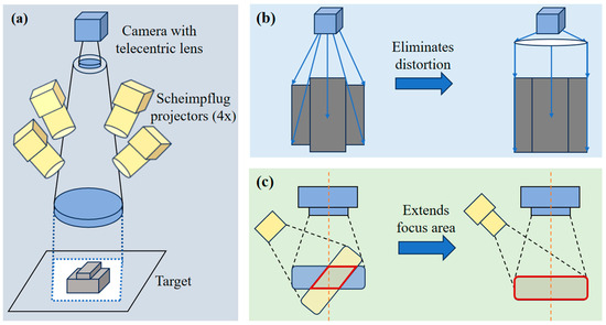
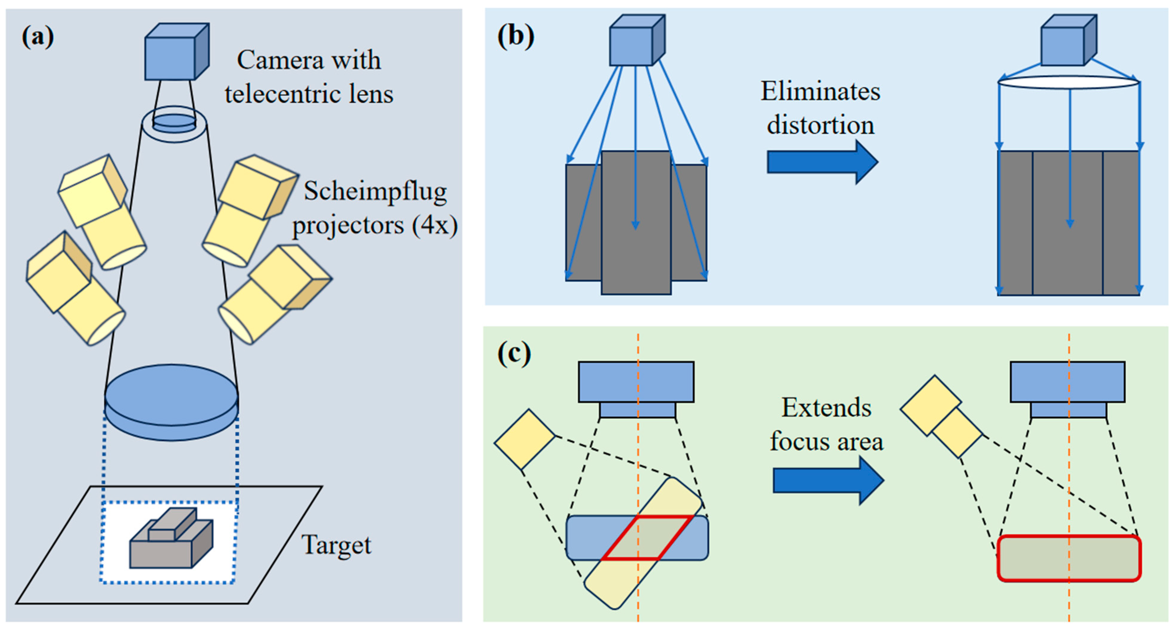
We focus on a specific multi-view configuration, namely a monocentric structured light system integrating a bilateral telecentric camera and four Scheimpflug projectors (custom built in-house), as illustrated in Figure 1a. This configuration is optically designed to alleviate visibility limitations by introducing multiple spatially distributed illumination directions, thereby improving surface coverage and robustness for complex geometries.
Figure 1.
Optical schematic of the system. (a) Monocentric camera with four Scheimpflug projectors. (b) Distortion-free imaging under telecentric projection. (c) Enlarged focus overlap area using Scheimpflug geometry.
The imaging module consists of a CXP camera (BC-GM65M12X4-M42, Bopixel, Beijing, China) with a pixel size of 3.2 μm × 3.2 μm, a resolution of 4800 × 4800, and a frame rate of 103.25 fps. It is equipped with a bilateral telecentric lens (DTCM71M-90-M58-AL, Vico Imaging, Hong Kong, China) featuring a magnification of 0.433, an object-space field of view of Ø90 mm, and a working distance of 208 mm. The image-space MTF exceeds 85 lp/mm, ensuring high-fidelity imaging. Crucially, the bilateral telecentric design enforces parallel chief rays in object space, which leads to parallel projection imaging. As a result, magnification remains constant regardless of object depth, and perspective distortion is effectively eliminated. Moreover, this parallel projection geometry suppresses occlusion-induced intensity variation, yielding shadow-free acquisition, as illustrated in Figure 1b. This property is particularly advantageous for phase measurement and reconstruction consistency.
To further enhance depth coverage, the system leverages the Scheimpflug principle in its projection geometry. Four DLP4710 (Texas Instrument, Dallas, TX, USA) projectors (1920 × 1080 resolution, orthogonal micromirror layout) are each equipped with lenses configured under the Scheimpflug condition, tilted by 4.48° along the Y-axis (with no tilt along X). This configuration inherently provides a tilt-shift capability, enabling coordinated alignment with the camera’s focal planes. As a result, the overlapping in-focus region between the camera and projectors is maximized, effectively expanding the confocal measurement volume, as shown in Figure 1c. Such an arrangement ensures that structured patterns remain sharply focused across a wider depth range, which is critical for accurate 3D reconstruction of non-planar surfaces.
For data acquisition, a hardware-synchronized pipeline is employed. Upon each trigger, the camera signals an FPGA board to generate sequential control signals, activating the four projectors in sequence. Each projector projects phase-shifted fringe patterns while the camera captures the corresponding images, ensuring strict temporal synchronization and consistent multi-view fringe acquisition.
2.2. FPP System Calibration
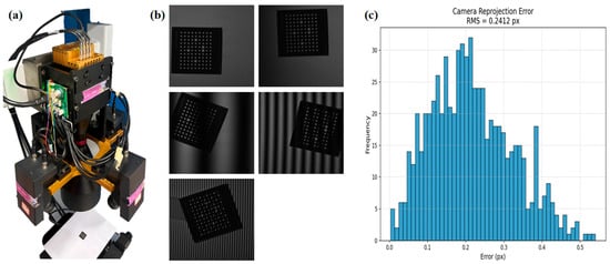
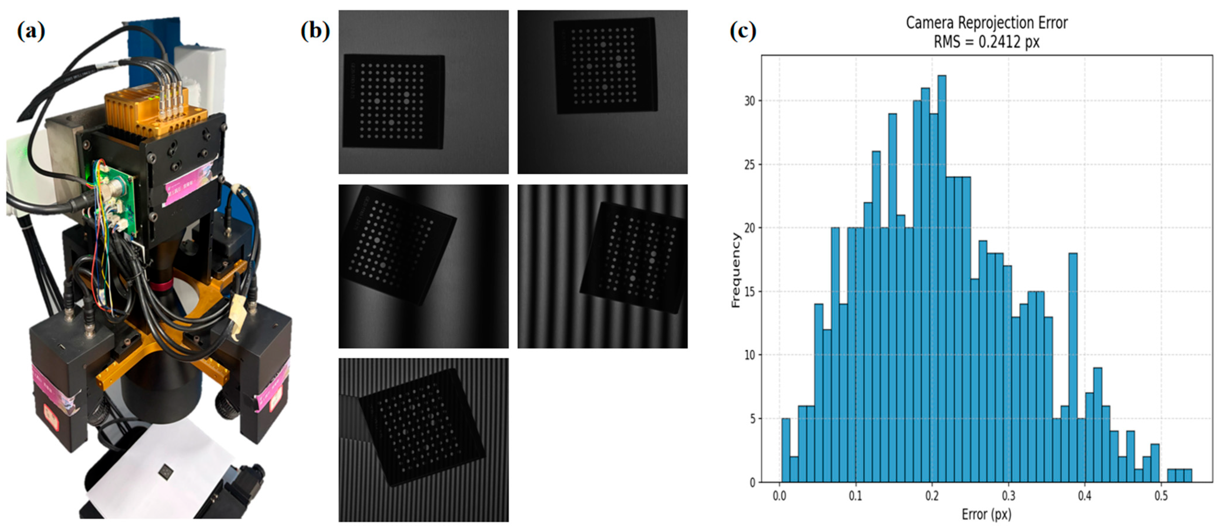
The calibration of the proposed multi-view FPP system is performed through an established unified multi-stage optimization framework, including intrinsic calibration, projector calibration, phase-based correspondence establishment, and global reprojection refinement. Figure 2a illustrates the complete physical setup; Figure 2b shows the calibration board and a few of its captured calibration images with fringe patterns.
Figure 2.
The multi-view FPP system and its camera calibration results. (a) The four-projector single-camera FPP system. (b) Representative calibration images captured under different projector illuminations and fringe patterns. (c) Reprojection error distributions of the camera.
First, the intrinsic parameters of the bilateral telecentric camera are calibrated using an adapted version of Zhang’s calibration method for telecentric imaging systems [30,32]. Unlike conventional perspective cameras, the telecentric lens maintains nearly constant magnification across depth variations and significantly suppresses perspective distortion. Therefore, the calibration model mainly focuses on accurately estimating the equivalent focal scaling factors and principal point parameters while minimizing residual distortion terms. The calibrated intrinsic parameters of the camera are summarized in Table 1. The recovered distortion coefficients remain very small, confirming the near-orthographic imaging characteristics of the telecentric optical system.
Table 1.
Calibration results of the FPP system.
For the four Scheimpflug projectors, a projector calibration strategy based on tilted imaging geometry is employed [33,34]. Specifically, the projector model establishes the mapping relationship between projector pixel coordinates and the corresponding spatial projection rays under Scheimpflug conditions. During calibration, each projector sequentially projects phase-shifting fringe patterns and coded patterns onto a planar calibration target containing circular feature arrays. The captured fringe images are then processed through phase calculation and phase unwrapping to establish dense pixel-wise correspondences between the camera and each projector.
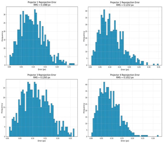
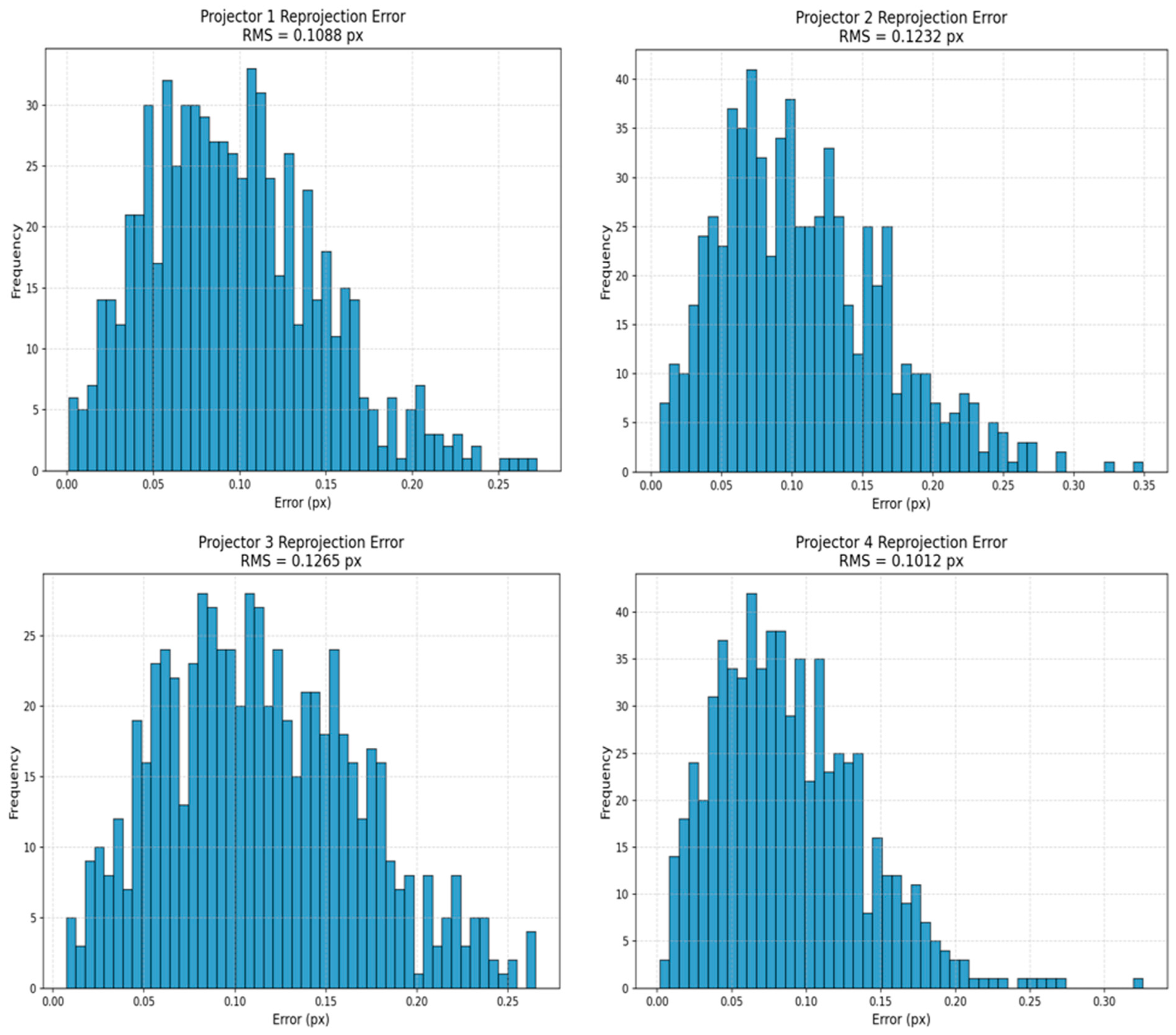
To improve calibration robustness and multi-view consistency, all camera-projector parameters are further refined through a global bundle-adjustment optimization. The optimization jointly minimizes the reprojection errors of all observed feature points across the four projection views while simultaneously refining intrinsic and extrinsic parameters. The resulting reprojection error distribution for the camera is shown in Figure 2c, and those for the projectors are shown in Figure 3. The camera achieves a mean reprojection error of approximately 0.2412 pixels, while the four projectors obtain average reprojection errors of approximately 0.1012, 0.1265, 0.1232, and 0.1088 pixels, respectively. The corresponding histograms indicate that the majority of reprojection residuals are concentrated within sub-pixel ranges, demonstrating high calibration accuracy and stable geometric consistency among all viewpoints.
Figure 3.
Reprojection error distributions of the four projectors.
The final calibrated extrinsic parameters further verify the spatial alignment of the multi-projector system. As listed in Table 1, the recovered translation vectors indicate that the four projectors are distributed around the central telecentric camera from different viewing directions, forming complementary observation baselines for occlusion suppression and multi-view geometric fusion. This calibration configuration provides accurate geometric constraints for the subsequent multi-view depth reconstruction and cross-view feature fusion processes.
2.3. Multi-View Fusion
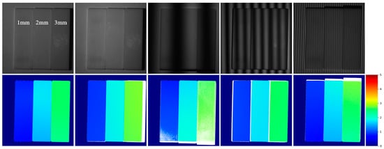
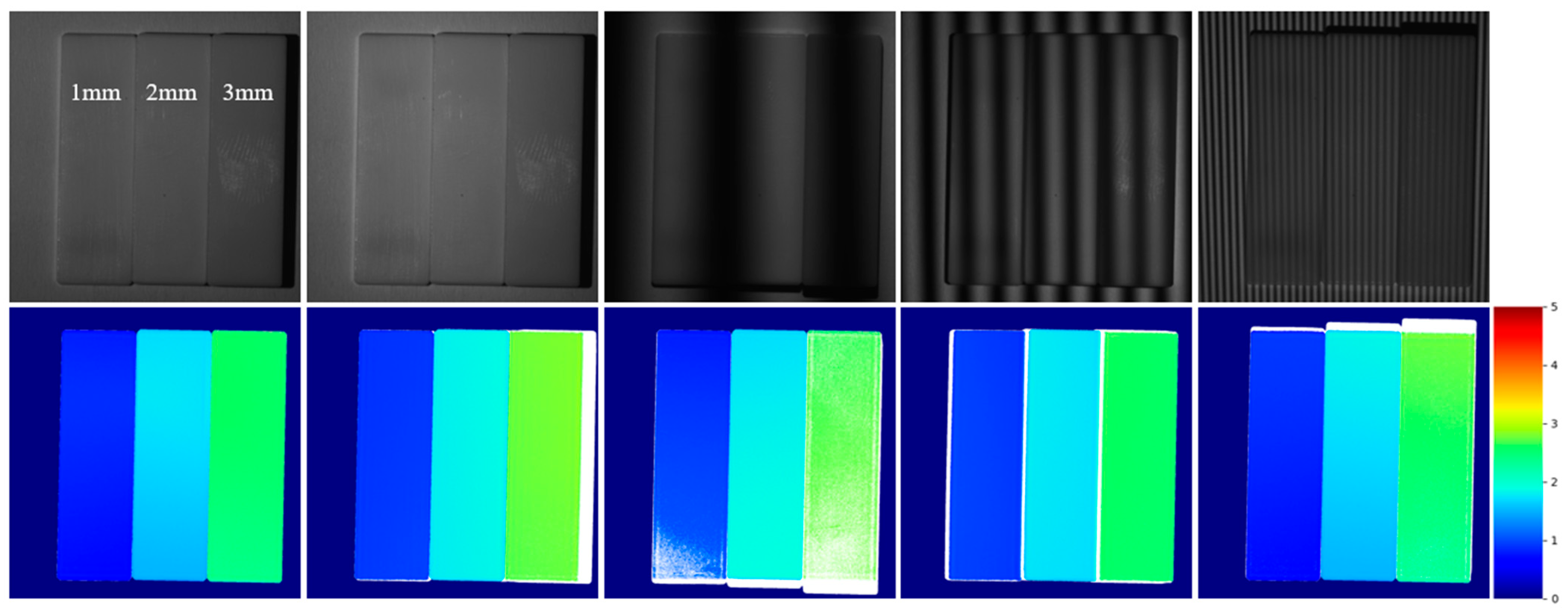
To evaluate the contribution of multi-view fusion, an experiment was conducted using a standard stepped object, which consists of three ceramic planar segments with precise thicknesses of 1 mm, 2 mm, and 3 mm, respectively. Figure 4 illustrates the experimental results.
Figure 4.
Qualitative evaluation of multi-view fusion. Top row: input fringe patterns from four directions (periods: 1, 8, 48, and 128) plus a grayscale reference. Bottom row: fused depth map (leftmost) and single-view depth maps.
The first row shows the fringe patterns projected onto the object by the four-view system. From left to right, these include: a conventional grayscale image under uniform illumination, a fringe pattern with period-1 from the right projector, a period-8 pattern from the top projector, a period-48 pattern from the left projector, and a period-128 pattern from the bottom projector. The reconstruction was performed using the multi-frequency heterodyne method, where the fringe images with multiple frequencies and phase shifts from each projector were individually processed to retrieve the unwrapped absolute phase. The corresponding depth maps are displayed in the second row. From left to right, these show: the fused depth map obtained by combining all four views, followed by the depth maps reconstructed solely from the right, top, left, and bottom projectors, respectively. In the single-view depth maps, the white regions represent shadowed areas where phase information could not be recovered; these shadowed regions are already evident as dark areas in the corresponding raw fringe images of the first row. The fused depth map, in contrast, effectively recovers the missing areas, producing a complete and accurate three-dimensional reconstruction. This comparison demonstrates that incorporating more views progressively mitigates occlusion and extends surface coverage. For objects with more complex geometries, the multi-view FPP offers clear advantages.
The above experimental results demonstrate the superiority of the multi-view FPP. However, the calibration of such a system remains challenging due to the complex interplay between the telecentric camera, multiple Scheimpflug projectors, and their spatial configuration. An alternative approach is to employ a DNN to directly learn the mapping between projection patterns and 3D coordinates, thereby circumventing the need for explicit physical modeling and intricate calibration procedures. This data-driven strategy offers a more flexible and unified solution, potentially addressing the limitations of conventional calibration in multi-view setups.
2.4. The Digital Twin of the FPP System and the Dataset
To overcome the practical difficulties of acquiring large-scale, precisely annotated real-world training data for such a system—a prerequisite for training robust DNNs—we developed a physically accurate simulation model within Blender. This virtual model is a digital twin of the physical FPP system, replicating its exact optical geometry, camera sensor characteristics, and projector illumination properties. This enables the generation of large, diverse datasets with perfect ground-truth 3D shapes, forming the foundation for the supervised learning of our proposed network, which will be detailed in the following sections. This combined strategy of physical prototyping and physics-based simulation ensures that the deep learning method is both practically grounded and optically consistent.
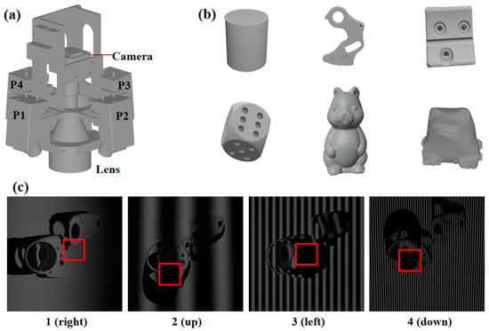
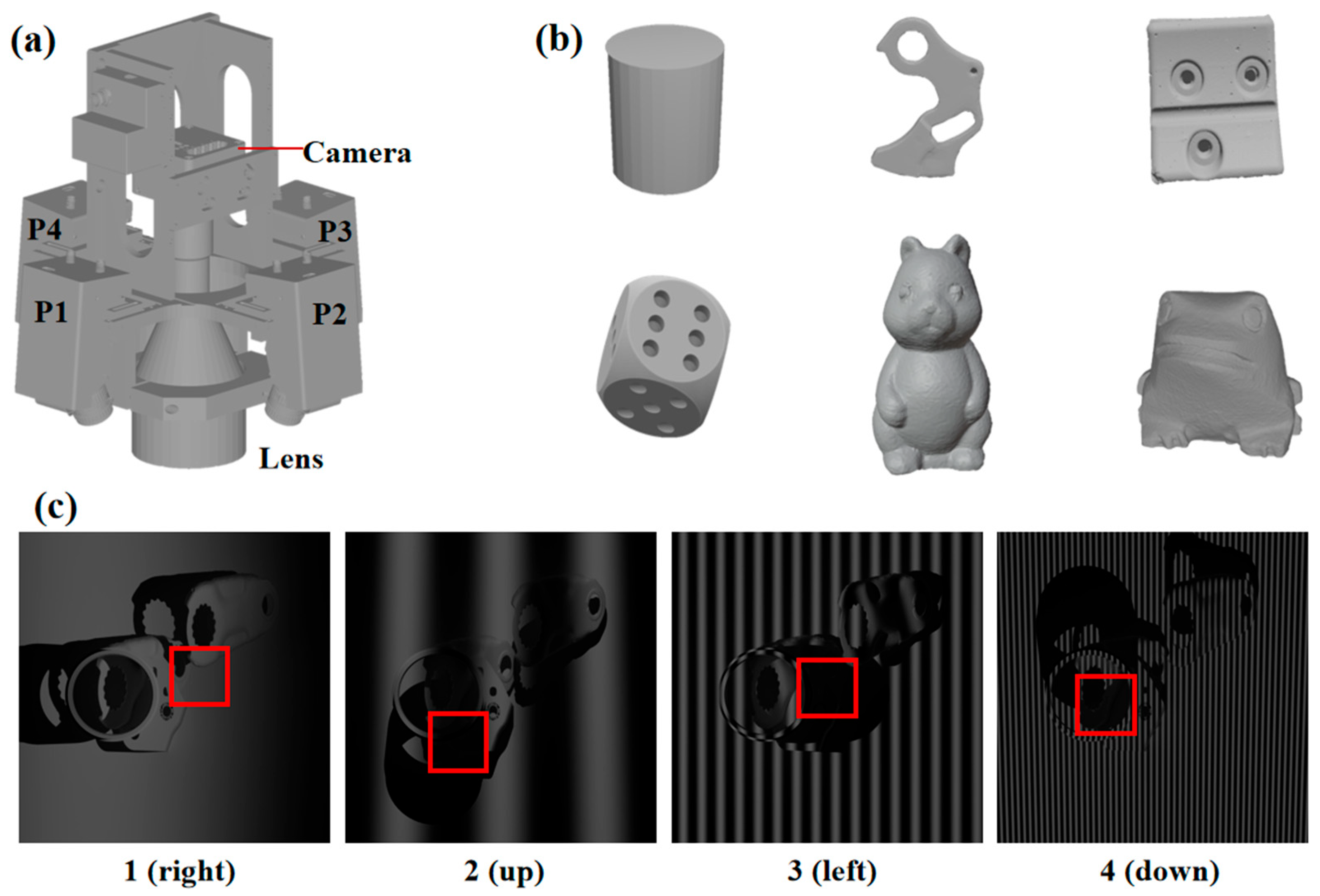
Blender’s advanced simulation capabilities enable not only flexible scene configuration but also subpixel-level precision in rendering, allowing the generation of highly realistic fringe patterns and accurate depth maps [35,36]. This level of control ensures that the synthetic dataset closely mimics real-world FPP acquisitions, providing a robust foundation for network training and quantitative evaluation. As depicted in Figure 5a, the central camera (4800 × 4800 pixels, 3.2 μm pixel pitch, and 35.47 mm × 35.47 mm field of view) is encircled by four projectors arranged in a cross pattern. These projectors illuminate objects from four directions—right, up, left, and down—labeled 1 through 4 in Figure 5c; each setting angle is 26 degrees with the optical axis of the camera, simulating the actual system tilt. Sinusoidal fringe patterns with phase shifts are projected to emulate real FPP hardware, while the camera incorporates realistic lens distortion and synthetic sensor noise to capture accurately deformed fringe images.
Figure 5.
The digital model of the multi-view FPP setup and dataset samples. (a) FPP hardware. (b) Sample objects for dataset generation. (c) Orthogonal fringe inputs with frequencies 1, 8, 48, and 128 highlighting projection shadows (red boxes) addressed by the proposed network.
To generate a comprehensive dataset suitable for training and evaluation, we rendered a high-quality multi-view FPP dataset in Blender. This synthetic framework allows precise ground-truth acquisition and reproducible performance testing. All rendered fringe images are stored in 32-bit OpenEXR format to avoid quantization loss, with depth information extracted directly from the Z-buffer [37]. The dataset encompasses a variety of object geometries, including simple primitives, mechanical components, and freeform shapes from Thingi10K [38], as shown in Figure 5b. Specifically, each scene contains a single composite object generated with equal probability either by merging 1–4 randomly scaled and rotated basic shapes (cube, sphere, and cylinder) or by merging 1–4 external CAD models from Thingi10K. Each merged object is assigned a random diffuse color, and with 30% probability, a metallic component (roughness: 0.2–0.5, metallic: 0.6–0.9) is added to increase reflectance diversity. Highly specular or transparent surfaces are not included in the current dataset, as they remain a challenging scenario for FPP. The dataset contains 252 scenes, with 4 views for each scene and 37 image sequences for each view (the total number of images is 37,296); each image sequence includes 1 uniform illumination and 18 horizontal and 18 vertical fringe patterns, where the 18 patterns contain 4 phase shift patterns from periods 1, 8, and 48 respectively (3 × 4 = 12), and 6 phase shift patterns for period 128.
As shown in Figure 5c, illumination from a single projector produces shadows due to occlusions (red boxes), which are mitigated by CVA-Net through complementary multi-view fusion, as detailed below. During network training, fringe sequences were represented using four orthogonal frequencies (1, 8, 48, and 128). To facilitate efficient computation, all images were downsampled to 480 × 480 via trilinear interpolation. The dataset was split into 80% for training, 10% for validation, and 10% for testing. Strict object-level separation was enforced among the splits: no CAD model or primitive combination used in the training set (202 scenes) appears in the validation (25 scenes) or test set (25 scenes), ensuring that the network’s performance reflects genuine generalization rather than memorization.
2.5. The Cross-View Attention Network
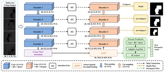
The proposed CVA-Net is an end-to-end multitask learning framework designed for depth reconstruction from multi-view fringe pattern inputs, as illustrated in Figure 6. The network adopts a unified 3D encoder–decoder architecture with shared parameters, enabling joint feature extraction and cross-view interaction within a single optimization pipeline. Given an input tensor of shape B × 1 × 4 × H × W, the model progressively encodes multi-view observations into hierarchical representations and reconstructs dense depth maps through a series of decoding stages, assisted by auxiliary supervision and iterative refinement. The design integrates a CVA module, an atrous spatial pyramid pooling (ASPP) [39], multi-scale depth outputs, and a global parameter estimation branch.
Figure 6.
The overall network structure of the CVA-Net.
The encoder consists of four hierarchical stages, each composed of a 3D convolutional layer followed by batch normalization, ReLU activation, and a residual block to enhance representation capacity while ensuring stable training [40]. Spatial downsampling is performed using anisotropic max pooling with a kernel size of 1 × 2 × 2, which reduces spatial resolution while preserving the view dimension. This allows the network to progressively capture geometric features from low-level fringe patterns to high-level structural representations. The decoder mirrors the encoder structure and restores spatial resolution via transposed convolutions. At each decoding stage, skip connections with attention gates (AG) are introduced to incorporate fine-grained features from the corresponding encoder stage [41,42,43]. The AG selectively emphasize informative regions and suppress irrelevant or noisy responses, conditioned on the decoder features.
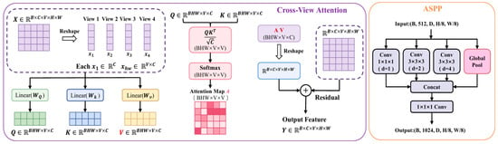
At the bottleneck of the encoder, the CVA module explicitly models dependencies across different viewpoints, as illustrated in Figure 7. For each spatial location, features from all views are treated as a sequence and processed using self-attention along the view dimension. Specifically, query, key, and value embeddings are generated via linear projections, and attention weights are computed via scaled dot-product attention as:
Figure 7.
The cross-view attention (CVA) and atrous spatial pyramid pooling (ASPP) modules for multi-view feature aggregation.
The aggregated features are then projected back to the original space and combined with the input through a residual connection. This mechanism enables adaptive fusion of complementary information across multiple viewpoints while preserving feature consistency. Following the CVA module, the 3D ASPP block captures multi-scale contextual information using multiple parallel dilated convolutions with different dilation rates, together with a global pooling branch, to enlarge the receptive field without sacrificing spatial resolution [44,45]. The outputs of all branches are concatenated and fused through a 1 × 1 × 1 convolution, generating a rich multi-scale feature representation that serves as the input to the decoder.
To facilitate stable training and improve prediction accuracy, the network produces depth maps at multiple scales. Auxiliary depth outputs are generated at intermediate decoding stages, while the final depth map is obtained from the last decoding layer via a convolution that collapses the view dimension. These multi-scale outputs provide additional supervision and help guide the learning process toward better convergence. In parallel, a parameter estimation branch is attached to the bottleneck features to regress a 55-dimensional global system parameter vector. This branch consists of 3D convolutional layers, followed by global average pooling and fully connected layers. The predicted vector encodes global geometric or system-level information, which serves as an auxiliary prior to guide depth refinement.
The network is trained using a composite multitask loss with deep supervision. The depth estimation loss is computed as a weighted combination of the structural similarity index measure (SSIM) loss and the L1 loss:
where α is a balancing factor, set to 0.8 in this study based on preliminary experimentation. This loss is applied to the final depth prediction as well as to the auxiliary outputs at different scales. The overall depth supervision is formulated as:
where the superscripts “main”, “aux1”, and “aux2” indicate the different depth output scales, and are the weighting factors. To better preserve edge information, an edge-aware loss is introduced by computing the L1 difference between the Sobel gradients of the predicted and ground-truth depth maps:
where and denote the predicted and ground-truth depth maps, respectively, and , represent Sobel operators along horizontal and vertical directions.
For the parameter branch, the vector contains the camera-intrinsic parameters plus the extrinsic parameters (rotation and translation) for the four projector-camera perspectives. The parameter loss is the sum of L1 losses on the intrinsic, rotation, and translation components:
where is the number of parameter groups (1 camera + 4 camera-projector combinations), and , , and denote intrinsic, rotation, and translation parameters, respectively. To enforce valid rotation representation, a quaternion unit-norm regularization term is introduced:
Finally, the total loss function is defined as:
where the weighing factors , , and are empirically determined. This multitask formulation jointly optimizes depth accuracy, structural consistency, edge sharpness, and global parameter consistency.
In summary, the proposed CVA-Net synergistically integrates three key design principles: (1) multi-view feature fusion via CVA, which explicitly models inter-view dependencies and adaptively aggregates complementary information to mitigate occlusion-induced blind zones; (2) multi-scale contextual aggregation through ASPP, which enlarges the receptive field and captures both fine local details and broader structural context; and (3) geometry-aware regularization via a multitask loss that jointly optimizes depth accuracy, edge sharpness, and global parameter consistency. The shared 3D encoder–decoder backbone processes all four views simultaneously, while the auxiliary parameter estimation branch provides implicit geometric priors without increasing inference cost [22,46]. This unified end-to-end framework directly learns to reconstruct complete, high-fidelity depth maps from multi-view fringe patterns, eliminating the need for explicit phase unwrapping, system calibration, or hand-crafted fusion rules.
3. Experimental Results
3.1. Experimental Setup
All experiments were run on a workstation with an Intel Core i7 CPU, an NVIDIA GeForce RTX 4090 GPU (24 GB VRAM), 64 GB RAM, and Ubuntu 20.04. The proposed network and all baselines were implemented in PyTorch 2.4.1 with CUDA 12.4. Automatic mixed precision (AMP) was used to accelerate training and inference. The network was trained for 200 epochs with a batch size of 2. The Adam optimizer (β1 = 0.9, β2 = 0.999) was applied with an initial learning rate of 1 × 10⁻⁴. A cosine annealing scheduler with warm restarts (period of 50 epochs) was used to stabilize convergence. Reconstruction accuracy was quantified using three metrics: mean absolute error (MAE), mean squared error (MSE), and root mean squared error (RMSE) [47]. These metrics were computed only over valid ground-truth pixels.
3.2. Fringe Pattern Period Experiment
In the proposed multi-view FPP, each projector independently projects sinusoidal fringe patterns onto the target object. For every acquisition, the network receives four groups of fringe images corresponding to the four projection directions, while all projectors share the same fringe period and initial phase configuration. Only the projection viewpoints differ. The fringe period, defined as the number of sinusoidal cycles distributed across the projected image, plays an important role in determining reconstruction accuracy and robustness. Generally, increasing the fringe period increases the spatial frequency of the projected patterns, allowing finer geometric details to be encoded. However, excessively dense fringes also make the phase estimation and unwrapping process more sensitive to noise, shadows, low-modulation regions, and surface discontinuities. To investigate the influence of fringe period on reconstruction performance, separate models were trained using fringe patterns with periods of 1, 8, 48, and 128, while keeping all other training settings identical.
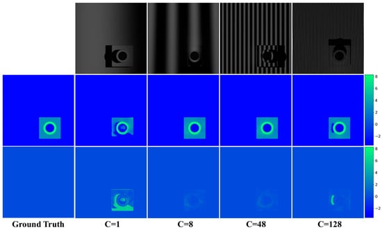
As shown in Figure 8, the model trained with period 1 produces the weakest reconstruction quality. Because the projected pattern contains only a very low-frequency intensity variation, the encoded geometric information is insufficient for accurately recovering local surface structures. Consequently, the predicted depth maps exhibit blurred boundaries and large reconstruction errors, as reflected by the error metrics reported in Table 2. When the fringe period increases to 8, the reconstruction accuracy improves significantly. The projected fringes provide sufficient spatial detail while still maintaining stable phase estimation in shadowed and discontinuous regions. As a result, the reconstructed depth maps exhibit clear structural boundaries and low error distributions. Quantitatively, period 8 achieves the best overall performance among all evaluated periods. Interestingly, the reconstruction results obtained with period 48 remain visually very similar to those of period 8. The predicted depth maps for periods 8 and 48 both preserve the main geometric structures and exhibit relatively low error distributions. However, the quantitative metrics of period 48 are slightly inferior, indicating that although higher-frequency fringes can still capture detailed geometry, they become more sensitive to local phase instability and noise, leading to small but measurable degradation in reconstruction consistency. When the fringe period further increases to 128, the reconstruction quality deteriorates more noticeably. The extremely dense fringe patterns increase the difficulty of reliable phase unwrapping, especially in regions affected by shadows, low fringe modulation, and abrupt depth changes. Consequently, the predicted depth maps contain larger local errors and reduced geometric stability.
Figure 8.
Impact of fringe period on reconstruction. From left to right: periods 1, 8, 48, and 128. (Top): input fringe images. (Middle): predicted depth maps. (Bottom): error maps relative to ground truth.
Table 2.
Reconstruction accuracy versus fringe period. Bold and underlined values indicate best results in each column.
Overall, periods 8 and 48 both provide strong reconstruction capability, with period 48 achieving performance close to that of period 8. Nevertheless, period 8 yields the best balance between geometric detail preservation and phase robustness, and is therefore selected as the default fringe period for all subsequent experiments. The predicted camera parameters corresponding to the period-8 configuration are provided in the Appendix A Table A2.
3.3. View Ablation Experiment
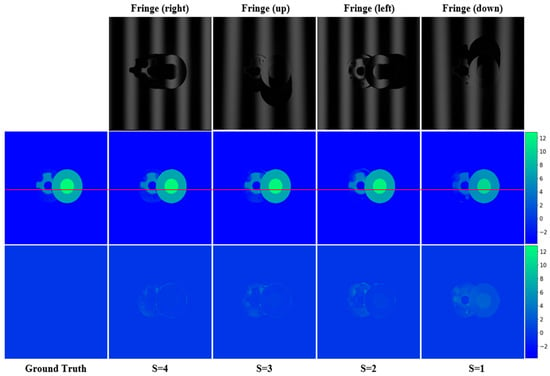
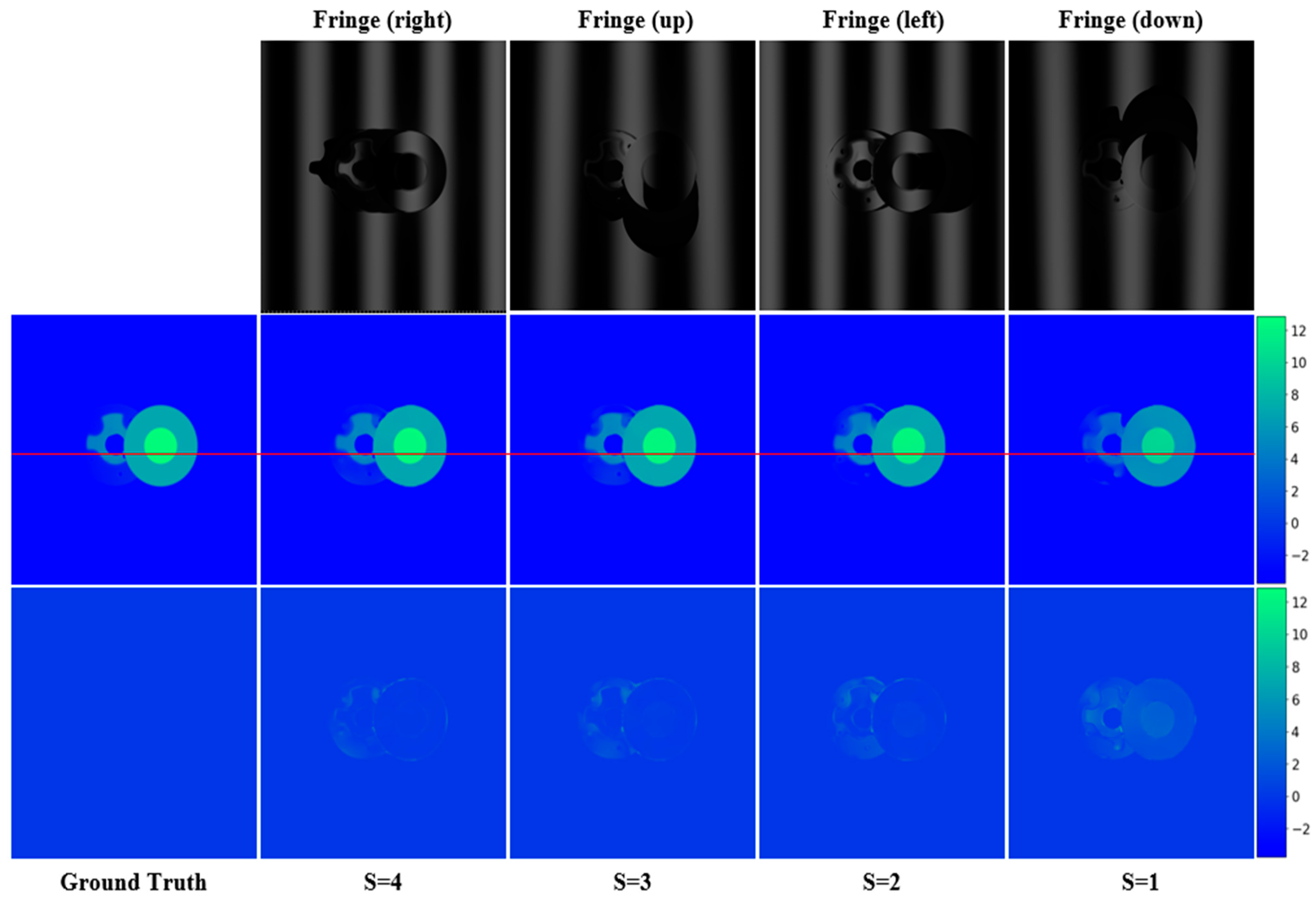
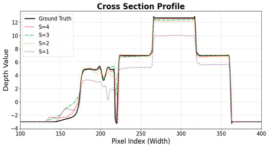
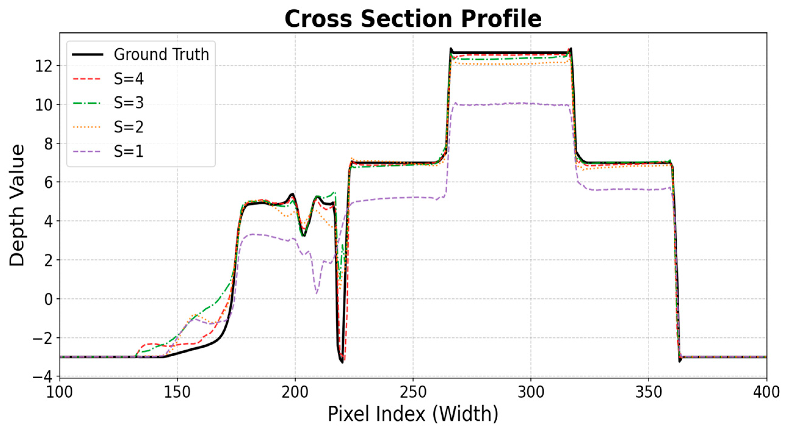
To systematically assess how the quantity of projection directions influences reconstruction completeness and accuracy, we performed a view ablation experiment by gradually increasing the number of input fringe sets fed into the network. The configurations range from a single projector (S = 1, right view only) to the full symmetric four-projector setup (S = 4, with projectors positioned at right, down, left, and up). All models were trained and evaluated under identical conditions. The results are shown in Figure 9 and Figure 10 and Table 3.
Figure 9.
View ablation: input fringe images (top), predicted depth maps (middle), and error maps (bottom) for S = 4 to S = 1. The red line indicates the cross-sectional scanline used for the depth profile comparison in Figure 10.
Figure 10.
Cross-section depth profile of the red line in Figure 9.
Table 3.
Reconstruction accuracy versus number of views. Bold values indicate best results in each column.
As expected, the single-view baseline (S = 1) suffers from fundamental visibility limitations. With illumination coming from only one direction, extensive shadow regions and self-occluded areas remain completely unreconstructed. The resulting depth map exhibits large holes and systematically elevated errors. Adding a second projector (S = 2, right and up) provides an orthogonal viewing pair. This configuration reduces the total blind area compared to the single-view case, but the reconstruction still contains noticeable artifacts. The two views are not sufficient to cover all concave regions or steep gradients, and some surface patches are captured by only one projector, leading to inconsistent depth estimates. Expanding to three projectors (S = 3, omitting the down view) yields a marked improvement. The network now receives fringe images from three distinct directions, which largely eliminate the major occluded zones present in the S = 2 case. Although the missing down view leaves a few residual shadow pockets, the overall depth map becomes substantially more complete, and the error metrics drop significantly. This result confirms that three well-distributed illumination directions can already capture most of the surface geometry.
The full four-view configuration (S = 4) achieves the best overall performance, with the lowest recorded errors (MAE = 0.0383 mm, MSE = 0.0387 mm2, and RMSE = 0.1967 mm). The predicted camera parameters corresponding to the S = 4 configuration are provided in Table A3 in the Appendix A. The symmetric arrangement of projectors along both horizontal and vertical axes ensures that every surface point is illuminated by at least one projection direction, and most points receive multiple phase measurements. The network fully exploits this redundancy to produce a seamless, hole-free depth map. The advantage of the symmetric layout is particularly evident in regions with complex topology or deep concavities, where the complementary observations from opposite sides effectively resolve ambiguities that would otherwise remain in asymmetric setups. Figure 10 presents quantitative depth profiles along the scanline marked in Figure 9, clearly illustrating the progressive improvement from S = 1 to S = 4 and the substantial gap in fidelity between the three-view and four-view configurations.
3.4. Network Module Ablation Experiment
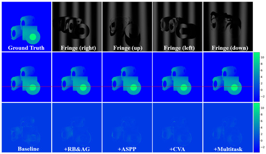
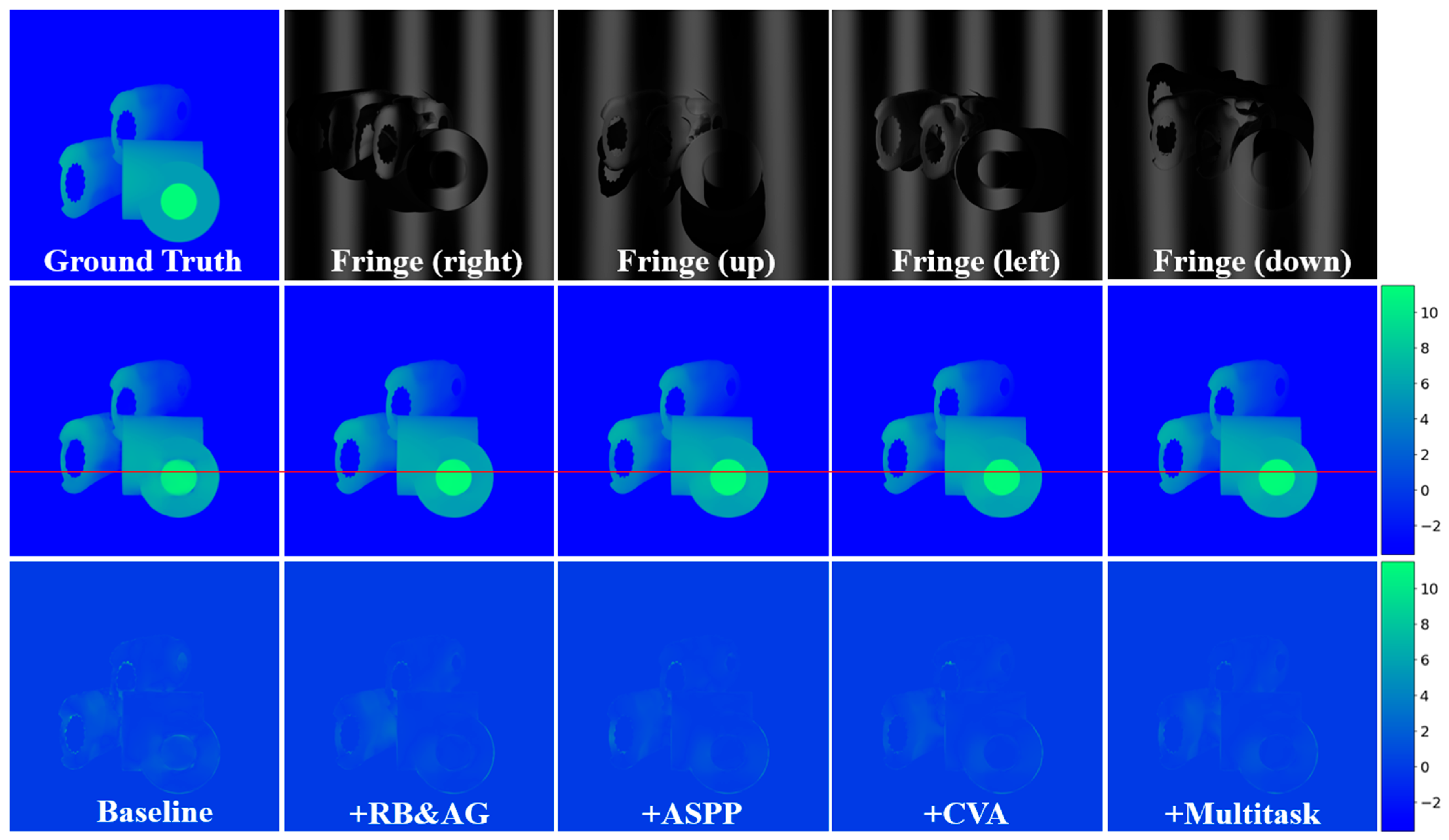
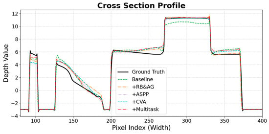
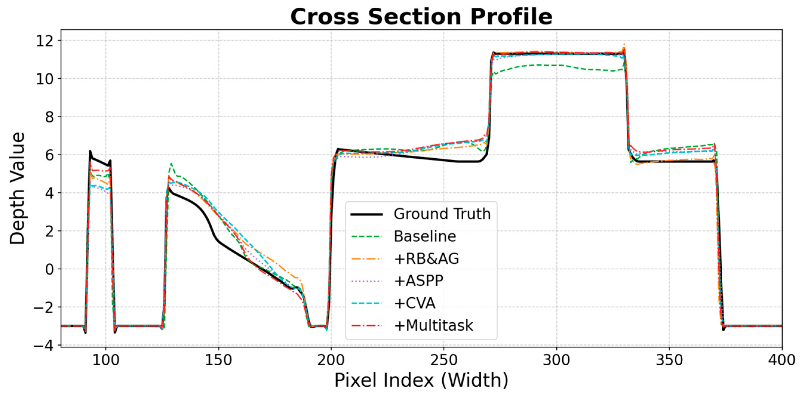
To dissect the contribution of each architectural component in the proposed CVA-Net, we conducted a systematic ablation study by progressively augmenting a standard 3D U-Net backbone with additional modules. The quantitative results of this analysis are summarized in Table 4, providing a comprehensive comparison of reconstruction accuracy across different model configurations. To further investigate the effect of each network component, Figure 11 presents visual reconstruction results and corresponding error maps for different ablated configurations. The first row shows the ground-truth depth map and the captured fringe patterns from four orthogonal projection directions. The second row illustrates the reconstructed depth maps obtained by progressively adding residual blocks (RB), AG, ASPP, and CVA modules and the multitask learning branch to the baseline network. The third row shows the corresponding error maps relative to the ground truth. As additional modules are incorporated, reconstruction quality improves progressively, while the magnitude and spatial extent of reconstruction errors are reduced. The corresponding depth profiles are presented in Figure 12. The profile traverses multiple discontinuities, curved surfaces, and occluded regions, providing a representative assessment of reconstruction fidelity.
Table 4.
Reconstruction accuracy of different network variants. Bold values indicate best results in each column.
Figure 11.
Visual comparison of module ablation experiments for CVA-Net. The red line indicates the cross-sectional scanline used for the depth profile comparison in Figure 12.
Figure 12.
Cross-section depth profile of the red line in Figure 11.
The study begins with the baseline configuration (vanilla 3D U-Net), which yields an initial MAE of 0.0622 mm. Incorporating residual blocks and attention gates (+RB&AG) results in a pronounced performance improvement, reducing the MAE to 0.0405 mm. This substantial gain indicates that residual connections effectively alleviate gradient degradation in deep feature hierarchies, while attention mechanisms enhance discriminative capacity by suppressing irrelevant background responses and emphasizing structurally salient regions. The attention gates, placed in the decoder, dynamically reweight encoder skip features, allowing the network to focus on fringe-rich areas and ignore shadowed or low-modulation regions.
The further integration of the ASPP module (+ASPP) leads to an additional improvement, achieving an MAE of 0.0401 mm. This result highlights the importance of multi-scale contextual aggregation for resolving geometric ambiguities, particularly in regions with limited texture or weak fringe contrast. By employing parallel dilated convolutions with varying receptive fields, ASPP effectively captures both fine-grained local details and broader structural context. This enables the network to better disambiguate depth estimation in homogeneous or low-texture areas where conventional single-scale convolutions tend to produce uncertain predictions.
The introduction of the CVA module (+CVA) further stabilizes high-dimensional feature interactions and improves cross-view consistency. The CVA module explicitly models relationships among the four view-specific feature volumes by computing attention weights across the view dimension. This design enables the network to dynamically aggregate complementary information from multiple projection directions, effectively learning to align and integrate multi-view features. By preserving the identity mapping via a residual connection within the CVA, the module ensures smooth gradient flow and stable training. With CVA, the MAE drops to 0.0387 mm, and the reconstruction completeness improves markedly, especially in occluded regions where only a subset of projectors provides reliable phase information.
Finally, extending the architecture to the full multitask learning framework (+Multitask) yields the best overall performance, with the MAE reaching 0.0383 mm. The auxiliary parameter prediction branch provides an additional geometric constraint by enforcing the network to learn high-level shape priors. This branch does not increase inference cost for depth prediction but supplies extra supervision during training. The improvement demonstrates that jointly optimizing auxiliary tasks acts as an effective global regularizer, enforcing high-level geometric constraints and promoting more robust and accurate 3D surface reconstruction. The full model outperforms all ablated variants.
3.5. Comparative Experiments
To benchmark the advantage of CVA-Net, we compared it against four representative single-frame depth estimation networks: UNet [48], hNet [49], UHRNet [50], and MTLNet [22], as well as a vanilla 3D U-Net baseline (denoted as “Baseline” below), as described in Section 3.4. These networks were originally designed for single-view structured light reconstruction, taking a single fringe image as input. To adapt them to the four-projector system, we modified the input layer of each network to accept four channels instead of one, corresponding to the fringe images from the four projectors (Right, Down, Left, and Up) stacked along the channel dimension. All other architectural components remained unchanged. This modification allows each baseline network to directly learn a mapping from the multi-view fringe patterns to a single depth map in an end-to-end manner, without requiring any post-fusion step.
During training, the input to each baseline network is a four-channel tensor (height × width × 4) formed by concatenating the fringe images from the four projectors. The ground-truth depth map remains at the camera-coordinate depth, which is shared across all views. At test time, each baseline network directly outputs a predicted depth map from the four-channel input. The predicted camera parameters corresponding to the CVA-Net configuration are provided in Table A4 in the Appendix A.
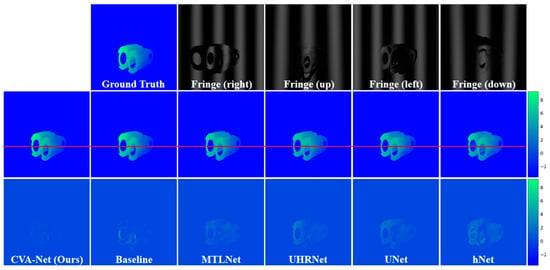
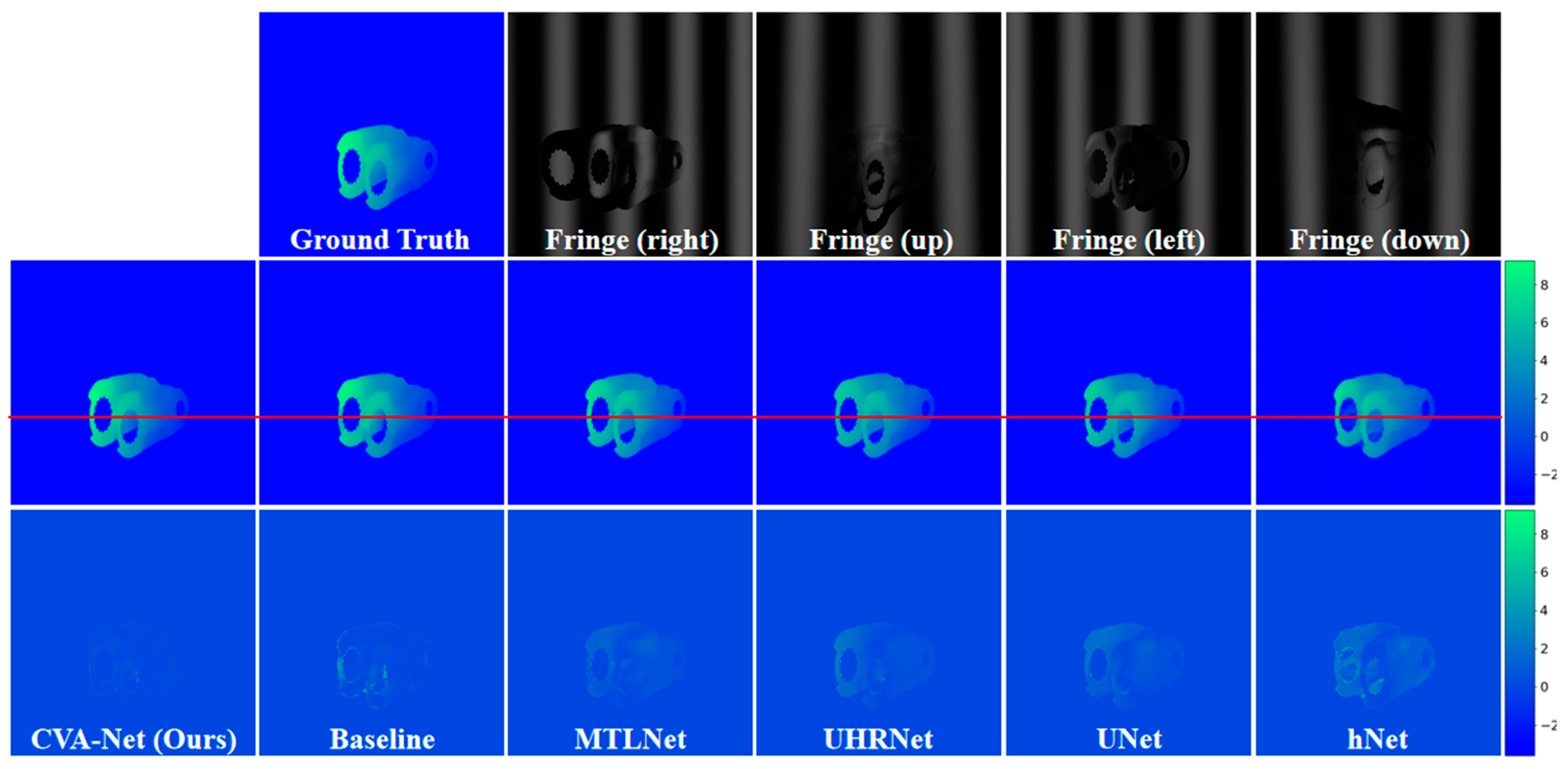
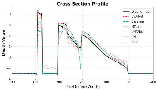
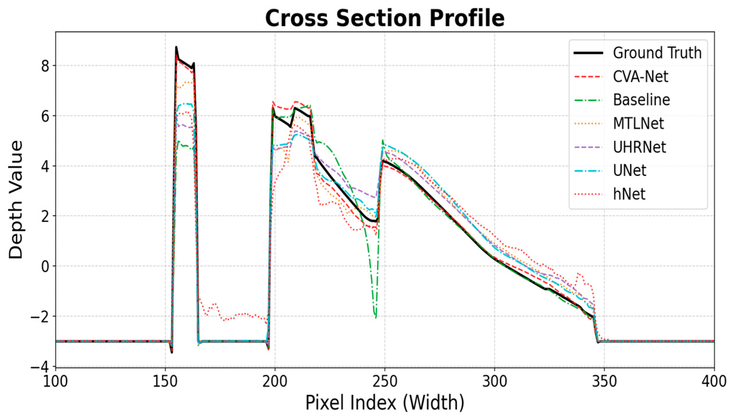
We performed comparative analyses of the reconstructed depth maps and their corresponding absolute error distributions. As illustrated in Figure 13 and Figure 14, and summarized quantitatively in Table 5, all five evaluated models are capable of recovering the global coarse morphology of the target object. However, pronounced differences emerge when assessing localized surface fidelity, boundary sharpness, and robustness in occluded regions.
Figure 13.
Comparison of depth reconstruction results by different deep learning models. The red line indicates the cross-sectional scanline used for the depth profile comparison in Figure 14.
Figure 14.
Cross-section depth profile of the red line in Figure 13.
Table 5.
Quantitative comparison of reconstruction accuracy. Bold and underlined values indicate the best and second best results in each column.
The baseline approaches exhibit clear limitations in reconstructing fine geometric structures and handling severe occlusion regions. hNet produces the weakest reconstruction performance, where the recovered surfaces contain obvious discontinuities, fragmented structures, and strong noise artifacts. Its corresponding MAE distribution also reveals large error concentrations over most structural regions, indicating poor geometric consistency. Although UNet improves the overall smoothness of the reconstructed surface, noticeable inaccuracies still remain around component edges and abrupt depth transitions, leading to unstable local reconstruction quality. UHRNet and MTLNet generate comparatively smoother depth maps and preserve more global structural information. In particular, MTLNet benefits from its multi-scale feature extraction capability, which enhances contextual representation. Nevertheless, both methods are inherently constrained by their single-view reconstruction paradigm. As a result, they struggle to recover reliable depth in heavily occluded or shadowed regions.
By contrast, the proposed CVA-Net achieves significantly more accurate and complete reconstructions through its collaborative four-view fusion framework. By aggregating complementary observations from multiple projection directions, the network effectively compensates for the visibility limitations of individual views and suppresses occlusion-induced artifacts. Consequently, the reconstructed surfaces exhibit improved continuity, sharper structural boundaries, and more reliable geometric topology. The superiority of CVA-Net is further verified through the depth-profile comparison shown in Figure 12. Along the selected scanline in Figure 11, the depth curve predicted by the proposed method closely follows the ground-truth profile with smooth and continuous variations. In comparison, the single-view methods exhibit obvious fluctuations, discontinuities, and local deviations caused by information loss in shadowed or low-modulation regions.
Quantitative comparisons in Table 5 further confirm the effectiveness of the proposed approach. CVA-Net achieves the best performance across all evaluation metrics, obtaining an MAE of 0.0383 mm, an MSE of 0.0387 mm2, and an RMSE of 0.1967 mm. Compared with MTLNet, which is the strongest competing single-view method, CVA-Net reduces the MAE, MSE, and RMSE by 64.3%, 82.4%, and 58.1%, respectively. These substantial improvements across multiple evaluation criteria highlight the effectiveness of the proposed multi-view fusion mechanism in overcoming occlusion interference and recovering high-fidelity surface details that are difficult to obtain using conventional single-view reconstruction networks.
3.6. Performance in the Presence of Noise
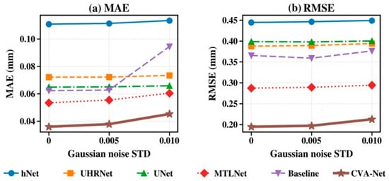
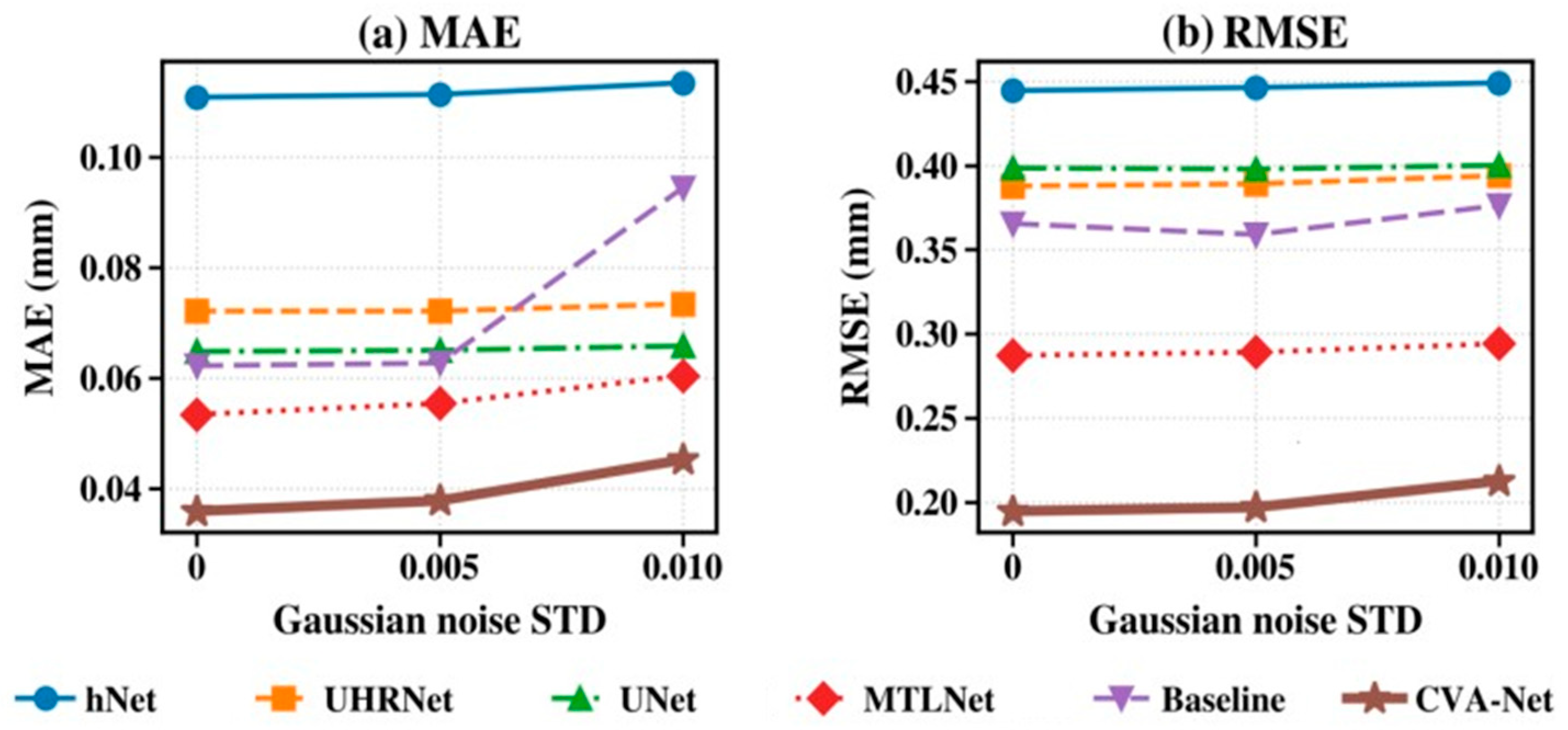
The comparison in Section 3.5 assumes the ideal case where no noise is taken into account. In real systems, sensor noise is inevitable. To evaluate the performance of the proposed CVA-Net for more realistic applications, two levels of zero-mean Gaussian noise are added to the input fringe pattern images (STD = 0.005 and STD = 0.01), and the same models are compared again. Table 6 summarizes the reconstruction results.
Table 6.
Quantitative comparison of reconstruction accuracy in the presence of zero-mean Gaussian noise. ∆MAE and ∆RMSE are percentage changes over the same value in Table 5. Bold and underlined values indicate the best and second best results in each column.
As expected, reconstruction accuracy generally decreases with increasing noise levels. The reconstruction errors with input images of both noise levels are greater than those with no-noise ones. Table 6 and Figure 15 also indicate that in the presence of mild Gaussian noise, UNet and UHRNet tend to be more robust, while the baseline (3D-UNet) is the least robust. CVA-Net’s robustness increases over the baseline, but it is not as robust as the other compared deep learning models. However, despite the increase in reconstruction errors, in absolute terms, CVA-Net still has the least errors in MAE and RMSE, and outperforms the other compared models significantly. For STD = 0.005, CVA-Net has 31.8% and 31.9% lower MAE and RMSE than the second-best MTLNet; for STD = 0.01, these values drop to 25.2% and 27.7% for MAE and RMSE, respectively.
Figure 15.
Reconstruction error changes with Gaussian noise levels. (a) MAE; (b) RMSE.
3.7. Physical FPP System Experiment
To further validate the practical applicability and Sim2Real generalization capability of the proposed CVA-Net, real-world experiments were conducted using the physical four-projector, single-camera FPP system in Figure 2. The test object was a standard printed circuit board (PCB) with a nominal thickness of 2 mm. The PCB contains complex surface structures, including fine conductive traces, solder pads, through-holes, and reflective metallic regions, which introduce severe challenges for fringe projection profilometry due to specular reflections, low-modulation areas, and sharp depth discontinuities.
In the experiment, fringe patterns were captured by the real hardware system, and the PCB 3D shape was measured using the same multi-frequency heterodyne phase-shifting method employed in the virtual system to obtain the ground truth depth map. The captured fringe images were then directly fed into different pre-trained reconstruction networks without any fine-tuning or domain adaptation. All compared networks were trained only on synthetic data generated from the Blender-based digital twin FPP system, enabling a strict evaluation of Sim2Real generalization performance.
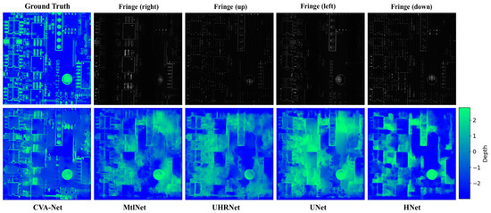
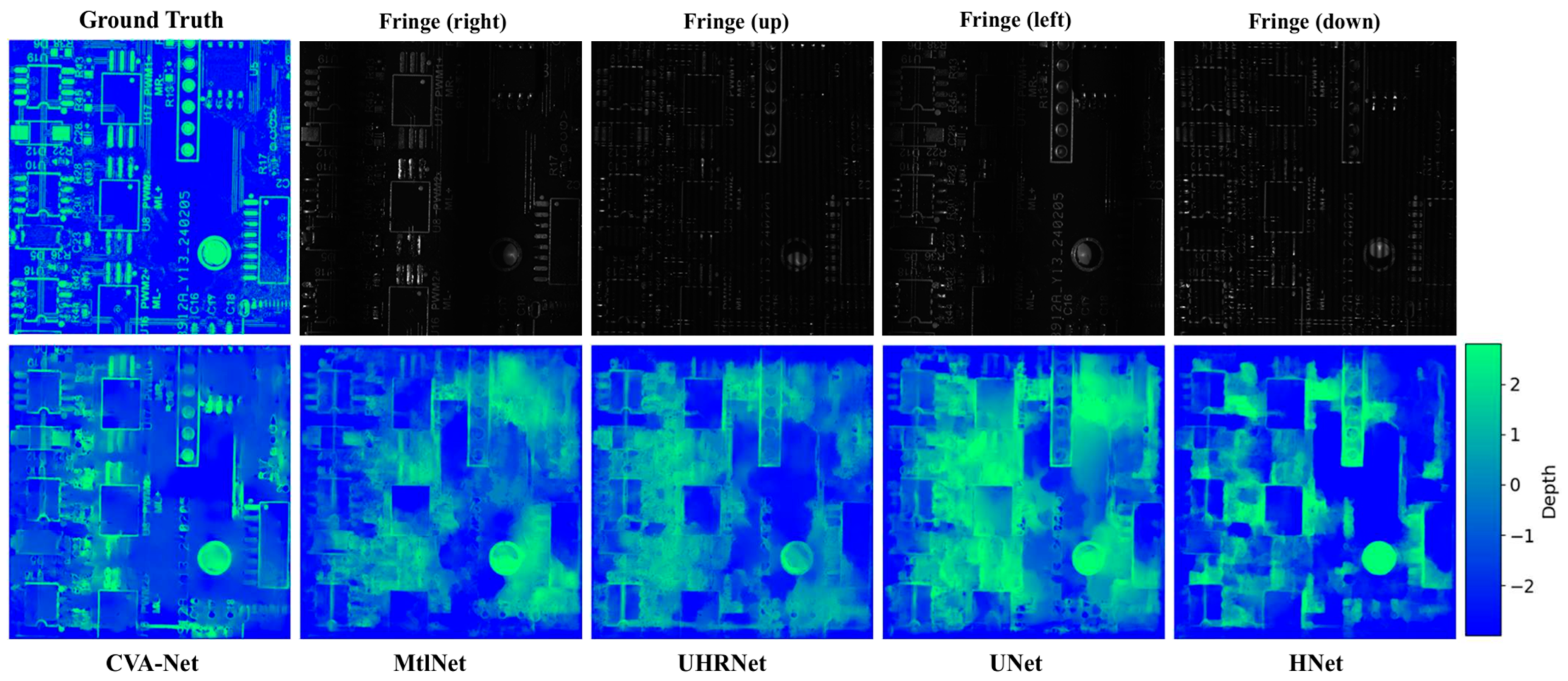
Figure 16 presents representative reconstruction results of different methods. The first row shows the captured fringe images under different projector illuminations. Due to the complex geometry and reflective characteristics of the PCB surface, each illumination direction exhibits different shadowed and low-contrast regions. The second row shows the depth reconstruction results produced by the compared methods. Among all methods, the proposed CVA-Net generates the most complete and structurally detailed depth map. Fine PCB structures, including chip boundaries, solder pads, connector holes, and circular metallic components, are reconstructed with clearer geometric continuity and sharper depth transitions. In contrast, the competing methods exhibit varying degrees of oversmoothing, local missing regions, blurred boundaries, and structural distortion. Specifically, MTLNet and UHRNet preserve partial geometric information but suffer from inconsistent local reconstruction and reduced edge sharpness. UNet produces relatively smooth results but loses fine structural details in high-frequency regions, while hNet exhibits noticeable artifacts and incomplete reconstruction in reflective and low-modulation areas.
Figure 16.
Comparison of PCB reconstruction results obtained by different methods on the physical FPP system (unit: mm).
Table 7 lists the quantitative errors of different reconstruction models on the PCB dataset. The proposed CVA-Net achieves the lowest MAE, MSE, and RMSE values among all compared methods, demonstrating the best overall reconstruction accuracy. It is worth noting that although hNet achieves relatively good numerical performance among the baseline methods, its reconstructed depth maps are visibly blurred and lack clear structural details. This indicates that lower error metrics do not necessarily correspond to better perceptual or geometric reconstruction quality, especially for objects containing fine structures and sharp edges. In contrast, the proposed CVA-Net not only achieves the best quantitative results but also produces more visually coherent and geometrically faithful reconstructions.
Table 7.
Quantitative comparison of reconstruction errors on real PCB measurements. Bold and underlined values indicate the best and second best results in each column.
Although the reconstruction errors are still not ideal under real imaging conditions, CVA-Net represents an important step to bridge the gap between virtual and real FPP systems. The experiments demonstrate that a network trained purely on synthetic data can successfully generalize to real captured fringe patterns without fine-tuning or domain adaptation. Future work will further consider practical factors such as sensor noise, illumination variation, projector-camera calibration errors, and more complex surface reflectance properties to improve the robustness and accuracy of real-world 3D reconstruction.
4. Conclusions and Discussion
In this study, we propose CVA-Net, a deep learning framework specifically designed to overcome the inherent occlusion and shadow limitations of single-view FPP by leveraging a symmetric four-view illumination setup. The core idea is to replace explicit geometric calibration and hand-crafted fusion rules with an end-to-end learnable architecture that directly predicts dense depth maps from multi-view fringe patterns. To enable this, we first built a Blender-based digital twin of the multi-view FPP system and generated a large-scale synthetic dataset with perfect ground-truth depth. Through extensive evaluations, we established that a fringe period of 8 provides the best trade-off between spatial resolution and robust phase unwrapping, and that the full four-view configuration yields the most complete and accurate reconstructions. The complete CVA-Net, incorporating residual blocks, attention gates, an ASPP block, a CVA module, and an auxiliary parameter estimation branch, outperforms state-of-the-art single-view networks (UNet, hNet, UHRNet, and MTLNet) by substantial margins. Real-world experiments on a PCB further demonstrate strong Sim2Real generalization, where CVA-Net successfully reconstructs fine details such as solder pads, conductive traces, and through-holes that other methods either miss or oversmooth. Taken together, CVA-Net establishes a state-of-the-art framework for multi-view FPP reconstruction, demonstrating that deep learning with explicit cross-view fusion offers a robust and occlusion-aware solution to the long-standing visibility limitations in 3D imaging. It is important to note, however, that physical calibration of the real FPP system is still required for acquiring ground-truth depth to evaluate real-world performance, and the digital twin used for training relies on a one-time geometric calibration. Once trained, CVA-Net performs calibration-free inference, offering a robust and occlusion-aware solution for multi-view 3D reconstruction.
Despite these achievements, several limitations remain. The current model relies on a 3D convolutional backbone with a large number of parameters and high GPU memory consumption, which may restrict real-time deployment on resource-constrained embedded platforms in industrial inspection. Moreover, although the Sim2Real training bridges the reality gap to a large extent, the robustness of the framework under extreme optical conditions—such as highly reflective or transparent surfaces, low-contrast fringes, or strong sensor noise—has not yet been fully explored. Regarding occlusion handling, while the proposed multi-projector setup effectively mitigates projection-related occlusions, camera-side occlusions—where the object itself blocks the camera’s view of a surface region—remain unresolved. Addressing these would require either a multi-camera system or a moving camera paradigm. Additionally, the present implementation assumes a fixed symmetric four-projector layout; adapting to unstructured or space-limited environments where projector placement must be changed dynamically remains an open challenge. Future work will aim to address these issues through model compression such as knowledge distillation, structured pruning, or lightweight attention mechanisms, self-supervised or weakly supervised learning paradigms that reduce dependence on dense ground truth annotations by exploiting cross-view photometric consistency, and the extension of the architecture with temporal modeling, e.g., recurrent units or spatiotemporal attention to enable high-fidelity reconstruction of moving or deforming objects.
Author Contributions
Conceptualization, Y.T.; methodology, Z.C., X.Z., and Y.T.; software, Z.C.; validation, Z.C.; formal analysis, Z.C.; investigation, X.Z.; resources, Y.T.; data curation, Z.C. and X.Z.; writing—original draft preparation, Z.C.; writing—review and editing, X.Z. and Y.T.; visualization, Z.C.; supervision, Y.T.; project administration, Y.T.; funding acquisition, X.Z. and Y.T. All authors have read and agreed to the published version of the manuscript.
Funding
This research was funded by the National Natural Science Foundation of China (No. 62327808), the Natural Science Foundation of Guangdong Province (No. 2023B0303000009), and the Shenzhen Talent Startup Funds (No. 827-000954).
Data Availability Statement
Data and code are available upon reasonable request to the corresponding author.
Conflicts of Interest
The authors declare no conflict of interest.
Abbreviations
The following abbreviations are used in this manuscript:
| FPM | Fringe projection profilometry |
| CVA | Cross-View Attention |
| ASPP | Atrous spatial pyramid pooling |
| MAE | Mean average error |
| MSE | Mean squared error |
| RMSE | Root mean squared error |
| DNN | Deep neural network |
| MTF | Modulation transfer function |
| AG | Attention gate |
| SSIM | Structural similarity index measure |
| PCB | Printed circuit board |
| Sim2Real | Simulation to reality |
Appendix A
The True Values of the Virtual System and the Predicted Values of Parameters in Each Experiment
Table A1.
The ground truth of blender system parameters.
Table A2.
The predicted camera parameters corresponding to the period-8 configuration in 4.1.
Table A3.
The predicted camera parameters corresponding to the S = 4 configuration in 4.2.
Table A4.
The predicted camera parameters corresponding to the CVA-Net configuration in 4.4.
References
- Zhang, Z.; Wang, H.; Li, Y.; Li, Z.; Gui, W.; Wang, X.; Zhang, C.; Liang, X.; Li, X. Fringe-Based Structured-Light 3D Reconstruction: Principles, Projection Technologies, and Deep Learning Integration. Sensors 2025, 25, 6296. [Google Scholar] [CrossRef] [Scilit] [PubMed]
- Sanchez-Torres, M.; Hernández-Capuchin, I.; Ramírez-Fernández, C.; Clemente, E.; Sánchez-González, J.L.J.; López-Martínez, A. Recent Advances in Digital Fringe Projection Profilometry (2022–2025): Techniques, Applications, and Metrological Challenges—A Review. Metrology 2026, 6, 3. [Google Scholar] [CrossRef] [Scilit]
- Feng, S.; Zhang, L.; Zuo, C.; Tao, T.; Chen, Q.; Gu, G. High dynamic range 3D measurements with fringe projection profilometry: A review. Meas. Sci. Technol. 2018, 29, 122001. [Google Scholar] [CrossRef] [Scilit]
- Marrugo, A.G.; Gao, F.; Zhang, S. State-of-the-art active optical techniques for three-dimensional surface metrology: A review. J. Opt. Soc. Am. A 2020, 37, B60–B77. [Google Scholar] [CrossRef] [Scilit] [PubMed]
- Van der Jeught, S.; Dirckx, J.J. Real-time structured light profilometry: A review. Opt. Lasers Eng. 2016, 87, 18–31. [Google Scholar] [CrossRef] [Scilit]
- Lv, S.; Huang, N.; Zou, Y.; Liu, C.; Long, S.Y.; Tang, D.; Jiang, X.; Kemao, Q. On the precision models of fringe projection profilometry: Unification, simplification and connection. Light Sci. Appl. 2026, 15, 232. [Google Scholar] [CrossRef] [Scilit] [PubMed]
- Gui, C.; Zhong, H.; Fu, Y.; Zhong, K.; Ma, B.; Yan, Z. A dual-projector three-dimensional measurement model for shading problem of micro-scale object complex surface. J. Mod. Opt. 2023, 70, 142–152. [Google Scholar] [CrossRef] [Scilit]
- Lv, S.; Kemao, Q. Modeling the measurement precision of Fringe Projection Profilometry. Light Sci. Appl. 2023, 12, 257. [Google Scholar] [CrossRef] [Scilit] [PubMed]
- Quan, C.; Chen, W.; Tay, C. Phase-retrieval techniques in fringe-projection profilometry. Opt. Lasers Eng. 2010, 48, 235–243. [Google Scholar] [CrossRef] [Scilit]
- Ordones, S.; Servin, M.; Padilla, M.; Choque, I.; Flores, J.L.; Muñoz, A. Shape defect measurement by fringe projection profilometry and phase-shifting algorithms. Opt. Eng. 2020, 59, 014107. [Google Scholar] [CrossRef] [Scilit] [PubMed]
- Chen, W.; Liu, Y.; Feng, S.; Yin, W.; Qian, J.; Li, Y.; Zhang, H.; Trusiak, M.; Kujawinska, M.; Chen, Q. Dual-frequency angular-multiplexed fringe projection profilometry with deep learning: Breaking hardware limits for ultra-high-speed 3D imaging. Opto-Electron. Adv. 2025, 8, 250021. [Google Scholar] [CrossRef] [Scilit]
- Zhou, L.; Li, Y.; Li, M.; Xiao, Y.; Feng, S. Fast fringe image denoising for 3D reconstruction using lightweight convolutional neural network. In Proceedings of the Conference on Spectral Technology and Applications (CSTA 2024); SPIE: Dalian, China, 2024. [Google Scholar]
- Liping, Z.; Xiaofeng, H.; Feiwen, P.; Bin, G.; Zai, L. Multi-modal denoising method for structured light 3D reconstruction under composite noise. Opto-Electron. Eng. 2026, 53, 250272-1–250272-19. [Google Scholar]
- Liu, X.; Yang, L.; Chu, X.; Zhou, L. A novel phase unwrapping method for binocular structured light 3D reconstruction based on deep learning. Optik 2023, 279, 170727. [Google Scholar] [CrossRef] [Scilit]
- Spoorthi, G.; Gorthi, S.; Gorthi, R.K.S.S. PhaseNet: A deep convolutional neural network for two-dimensional phase unwrapping. IEEE Signal Process. Lett. 2018, 26, 54–58. [Google Scholar]
- Sumanth, K.; Ravi, V.; Gorthi, R.K. A multi-task learning for 2D phase unwrapping in fringe projection. IEEE Signal Process. Lett. 2022, 29, 797–801. [Google Scholar] [CrossRef] [Scilit]
- Trusiak, M.; Kujawinska, M. Deep learning enabled single-shot absolute phase recovery in high-speed composite fringe pattern profilometry of separated objects. Opto-Electron. Adv. 2023, 6, 230172-1–230172-4. [Google Scholar] [CrossRef] [Scilit]
- Zhu, X.; Lan, T.; Zhao, Y.; Wang, H.; Song, L. End-to-end color fringe depth estimation based on a three-branch U-net network. Appl. Opt. 2024, 63, 7465–7474. [Google Scholar] [CrossRef] [Scilit]
- Zhang, Z.; Li, Y.; Han, Z.; Zhang, C.; Liang, X.; Li, X. An End-to-End Network for 3D Reconstruction from Multi-Frequency Fringe Patterns. In Proceedings of the 2025 IEEE 26th China Conference on System Simulation Technology and its Applications (CCSSTA); IEEE: Piscataway, NJ, USA, 2025. [Google Scholar]
- Li, Y.; Qian, J.; Feng, S.; Chen, Q.; Zuo, C. Deep-learning-enabled dual-frequency composite fringe projection profilometry for single-shot absolute 3D shape measurement. Opto-Electron. Adv. 2022, 5, 210021-1–210021-16. [Google Scholar] [CrossRef] [Scilit]
- Machineni, R.C.; Spoorthi, G.; Vengala, K.S.; Gorthi, S.; Gorthi, R.K.S.S. End-to-end deep learning-based fringe projection framework for 3D profiling of objects. Comput. Vis. Image Underst. 2020, 199, 103023. [Google Scholar] [CrossRef] [Scilit]
- Zhong, X.; Huang, J.; Li, Y.; Chen, J.; Tian, Y.; Wu, Z. Single-shot fringe projection profilometry based on multi-task learning: Efficient depth reconstruction without explicit system calibrations. Phys. Scr. 2025, 100, 026005. [Google Scholar] [CrossRef] [Scilit]
- Qian, J.; Feng, S.; Li, Y.; Tao, T.; Han, J.; Chen, Q.; Zuo, C. Single-shot absolute 3D shape measurement with deep-learning-based color fringe projection profilometry. Opt. Lett. 2020, 45, 1842–1845. [Google Scholar] [CrossRef] [Scilit] [PubMed]
- Li, H.; Zhong, Y.; Liao, Z.; Zhang, X. High-accuracy calibration and efficient 3D reconstruction of a dual-camera telecentric structured light vision system. Opt. Laser Technol. 2025, 192, 114089. [Google Scholar] [CrossRef] [Scilit]
- Fu, Y.; Luo, L.; Zhong, K.; Li, F. High-accuracy fringe projection profilometry without phase unwrapping based on multi-view geometry constraints. Opt. Express 2024, 32, 38449–38464. [Google Scholar] [CrossRef] [Scilit] [PubMed]
- Zhang, G.; Liu, Y.; Yao, Q.; Deng, H.; Zhao, H.; Zhang, Z.; Yang, S. Multi-view fringe projection profilometry for surfaces with intricate structures and high dynamic range. Opt. Express 2024, 32, 19146–19162. [Google Scholar] [CrossRef] [Scilit] [PubMed]
- Dickins, A.; Widjanarko, T.; Sims-Waterhouse, D.; Thompson, A.; Lawes, S.; Senin, N.; Leach, R. Multi-view fringe projection system for surface topography measurement during metal powder bed fusion. J. Opt. Soc. Am. A 2020, 37, B93–B105. [Google Scholar] [CrossRef] [Scilit] [PubMed]
- Deetjen, M.E.; Lentink, D. Automated calibration of multi-camera-projector structured light systems for volumetric high-speed 3D surface reconstructions. Opt. Express 2018, 26, 33278–33304. [Google Scholar] [CrossRef] [Scilit] [PubMed]
- Yang, H.; Fang, C.; Zhang, X. Improvement of calibration method for multi-camera line structured light vision system. Appl. Physics. B Lasers Opt. 2022, 128, 116. [Google Scholar] [CrossRef] [Scilit]
- Zhang, G.; Cui, K.; Ji, P.; Tian, Y.; Yang, S. Calibration method for multiview telecentric fringe projection profilometry system. In Proceedings of the Emerging Digital Micromirror Device-Based Systems and Applications XVIII; SPIE: Schiedam, The Netherlands, 2026; pp. 93–100. [Google Scholar]
- Chen, Z.; Zhong, X.; Tian, Y. UARNet-3D: Deep learning-based multiview 3D reconstruction for fringe projection profilometry. In Proceedings of the Emerging Digital Micromirror Device-Based Systems and Applications XVIII; SPIE: Schiedam, The Netherlands, 2026. [Google Scholar]
- Zhang, Z. A flexible new technique for camera calibration. IEEE Trans. Pattern Anal. Mach. Intell. 2000, 22, 1330–1334. [Google Scholar] [CrossRef] [Scilit]
- Deng, H.; Hu, P.; Zhang, G.; Xia, C.; Cai, Y.; Yang, S. Accurate and flexible calibration method for a 3D microscopic structured light system with telecentric imaging and Scheimpflug projection. Opt. Express 2023, 31, 3092–3113. [Google Scholar] [CrossRef] [Scilit] [PubMed]
- Yang, Y.; Zhang, S. Pixelwise calibration method for a telecentric structured light system. Appl. Opt. 2024, 63, 2562–2569. [Google Scholar] [CrossRef] [Scilit] [PubMed]
- Zhu, X.; Zhang, Z.; Hou, L.; Song, L.; Wang, H. Light field structured light projection data generation with Blender. In Proceedings of the 2022 3rd International Conference on Computer Vision, Image and Deep Learning & International Conference on Computer Engineering and Applications (CVIDL & ICCEA); IEEE: Piscataway, NJ, USA, 2022. [Google Scholar]
- Mildenhall, B.; Srinivasan, P.P.; Tancik, M.; Barron, J.T.; Ramamoorthi, R.; Ng, R. Nerf: Representing scenes as neural radiance fields for view synthesis. Commun. ACM 2021, 65, 99–106. [Google Scholar] [CrossRef] [Scilit]
- Kainz, F.; Bogart, R.; Hess, D. The OpenEXR image file format. ACM SIGGRAPH Tech. Sketches 2003, 2, 26. [Google Scholar]
- Zhou, Q.; Jacobson, A. Thingi10k: A dataset of 10,000 3d-printing models. arXiv 2016, arXiv:1605.04797. [Google Scholar]
- Weber, M.; Wang, H.; Qiao, S.; Xie, J.; Collins, M.D.; Zhu, Y.; Yuan, L.; Kim, D.; Yu, Q.; Cremers, D. Deeplab2: A tensorflow library for deep labeling. arXiv 2021, arXiv:2106.09748. [Google Scholar]
- Wu, C.; Qiao, Z.; Zhang, N.; Li, X.; Fan, J.; Song, H.; Ai, D.; Yang, J.; Huang, Y. Phase unwrapping based on a residual en-decoder network for phase images in Fourier domain Doppler optical coherence tomography. Biomed. Opt. Express 2020, 11, 1760–1771. [Google Scholar] [CrossRef] [Scilit] [PubMed]
- Deng, W.; Shi, Q.; Li, J. Attention-gate-based encoder–decoder network for automatical building extraction. IEEE J. Sel. Top. Appl. Earth Obs. Remote Sens. 2021, 14, 2611–2620. [Google Scholar] [CrossRef] [Scilit]
- Chen, S.; Cheng, Z.; Zhang, L.; Zheng, Y. SnipeDet: Attention-guided pyramidal prediction kernels for generic object detection. Pattern Recognit. Lett. 2021, 152, 302–310. [Google Scholar] [CrossRef] [Scilit]
- Hou, Q.; Zhou, D.; Feng, J. Coordinate attention for efficient mobile network design. In Proceedings of the IEEE/CVF Conference on Computer Vision and Pattern Recognition; IEEE: Piscataway, NJ, USA, 2021. [Google Scholar]
- Dewi, C.; Chen, R.-C.; Yu, H.; Jiang, X. Robust detection method for improving small traffic sign recognition based on spatial pyramid pooling. J. Ambient Intell. Humaniz. Comput. 2023, 14, 8135–8152. [Google Scholar]
- Prudviraj, J.; Vishnu, C.; Mohan, C.K. M-FFN: Multi-scale feature fusion network for image captioning. Appl. Intell. 2022, 52, 14711–14723. [Google Scholar] [CrossRef] [Scilit]
- Thung, K.-H.; Wee, C.-Y. A brief review on multi-task learning. Multimed. Tools Appl. 2018, 77, 29705–29725. [Google Scholar] [CrossRef] [Scilit]
- Allen, D.M. Mean square error of prediction as a criterion for selecting variables. Technometrics 1971, 13, 469–475. [Google Scholar] [CrossRef]
- Ronneberger, O.; Fischer, P.; Brox, T. U-net: Convolutional networks for biomedical image segmentation. In Proceedings of the 18th International Conference on Medical Image Computing and Computer-Assisted Intervention (MICCAI), Munich, Germany, 5–9 October 2015; Springer: Berlin/Heidelberg, Germany, 2015; pp. 234–241. [Google Scholar]
- Nguyen, H.; Ly, K.L.; Tran, T.; Wang, Y.; Wang, Z. hNet: Single-shot 3D shape reconstruction using structured light and h-shaped global guidance network. Results Opt. 2021, 4, 100104. [Google Scholar] [CrossRef] [Scilit]
- Wang, Y.; Zhou, C.; Qi, X.; Li, H. UHRNet: A deep learning-based method for accurate 3D reconstruction from a single fringe-pattern. J. Mod. Opt. 2023, 70, 707–722. [Google Scholar] [CrossRef] [Scilit]

Disclaimer/Publisher’s Note: The statements, opinions and data contained in all publications are solely those of the individual author(s) and contributor(s) and not of MDPI and/or the editor(s). MDPI and/or the editor(s) disclaim responsibility for any injury to people or property resulting from any ideas, methods, instructions or products referred to in the content. |
© 2026 by the authors. Licensee MDPI, Basel, Switzerland. This article is an open access article distributed under the terms and conditions of the Creative Commons Attribution (CC BY) license.