Cascaded Fiber-Optic Time Synchronization System with Different Modulation Format

Abstract

High-precision time and frequency transfer plays a pivotal role in metrology, geodesy, deep-space exploration and other scientific applications. Based on current time synchronization research, extending point-to-point schemes into a wide-area network can significantly increase the range of applications. Therefore, we design and implement a cascaded fiber optic time synchronization system, which is the most basic form of networking. This paper considers two different modulation formats for time synchronization systems from the perspective of fiber nonlinear effects, namely the intensity modulation with direct detection (IMDD) scheme and the phase modulation with self-coherent detection (PMSCD) scheme. The analysis indicates that the constant-envelope characteristic of the PMSCD scheme provides superior transmission performance. Accordingly, we deployed the PMSCD system over a 500 km intercity fiber link and the IMDD system over a 68 km metropolitan fiber link, forming a 568 km cascaded system that achieves time synchronization precision better than 50 ps. This work offers a practical reference for the future development of high-precision fiber-optic time and frequency synchronization networks.

1. Introduction

Ultra-stable time–frequency reference signals are of vital importance in a wide spectrum of application fields, including metrology applications [1,2,3], navigation and positioning [4,5,6], and fundamental physics research [7,8,9,10]. Presently, Global Navigation Satellite Systems (GNSS) serve as the mainstream scheme for large-scale time–frequency synchronization. The Global Positioning System (GPS), the Beidou Navigation Satellite System (BDS) and other constellations are capable of stable positioning, navigation, and timing (PNT) services [11,12]. However, due to limitations such as ionospheric disturbances and multipath effects, the real-time timing precision of GNSS is generally confined to the nanosecond level. As the core of modern communication infrastructures, fibers can offer large bandwidth, low transmission loss, and high resilience to electromagnetic interference, making them an excellent medium for long-distance signal transmission. Moreover, fiber can be used as an analog channel, endowing it with a higher precision and more reliable capacity for carrying time and frequency signals compared to microwave channels [13,14,15]. Consequently, high-precision time and frequency transfer via long-distance fiber links has emerged as a prominent research focus, complementing and extending the capabilities of satellite-based methods.

Despite the superior timing accuracy delivered by analog fiber-optic time and frequency transmission systems, they exhibit poor compatibility with existing digital fiber-optic communication systems for the following reasons. First, high-precision time and frequency transfer typically relies on bidirectional transmission over a single fiber to exploit path reciprocity for delay measurement and compensation [16,17]. This approach conflicts with the dual-fiber bidirectional architecture commonly used in digital communication systems [18,19]. Second, since time and frequency signals are highly sensitive to transmission delay, they must be processed and compensated at the physical layer and cannot be readily integrated as a service into higher-level communication protocols. Consequently, analog time and frequency transfer networks cannot fully leverage existing digital communication infrastructure—including both hardware and protocols—and require additional specialized designs.

In recent years, numerous institutions worldwide have begun constructing ground-based fiber-optic time–frequency networks. For instance, the Clock Network Services-Design Study (CLONETS-DS) project, which is funded by the European Union, seeks to establish a pan-European reference system for time and frequency [20]. The REFIMEVE project, led by LNE-SYRTE, delivers high-precision time–frequency signals to research institutions across France, Germany, and the United Kingdom [21]. China’s National Time Service Center (NTSC) has arranged to build a terrestrial ultra-precision timing service infrastructure, with an overall optical fiber coverage spanning 20,000 km. The relevant experiments were carried out over a 1839 km fiber optic link from Xi’an to other cities [22,23,24]. Moreover, some researchers have already begun to conduct further studies on the topology of fiber-optic time and frequency networks [25]. If a fiber-optic time synchronization network is decomposed into a clock-difference measurement–compensation subsystem and a signal transmission subsystem, it becomes evident that most existing studies focus predominantly on the former, with relatively limited attention devoted to the latter. Since the stability of the time signal received by end users depends on the performance of both subsystems, we argue that the design of a high-performance and cost-effective signal transmission subsystem is equally critical in fiber-optic time synchronization networks.

After comprehensively considering factors such as system performance, transmission distance, and cost, we propose a networking strategy that employs phase modulation–self-coherent detection (PMSCD) for long-haul links and intensity modulation–direct detection (IMDD) for short-range transmission. The former is intended primarily for intercity or interprovincial connections, while the latter targets metropolitan-area fiber links. In general, complex fiber-optic time–frequency networks often incorporate multiple topological structures—such as tree, star, and ring configurations. This paper focuses specifically on cascaded time synchronization systems, which are widely used to interconnect different hierarchical levels within time synchronization networks or to integrate various topologies into more complex architectures [26,27,28,29]. Given their practical relevance, we believe that the proposed hybrid-modulation cascaded networking approach offers broad applicability and serves as a valuable reference for future implementations.

2. Principle

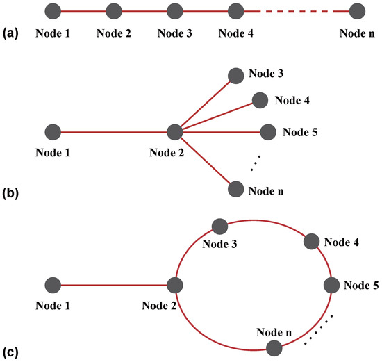
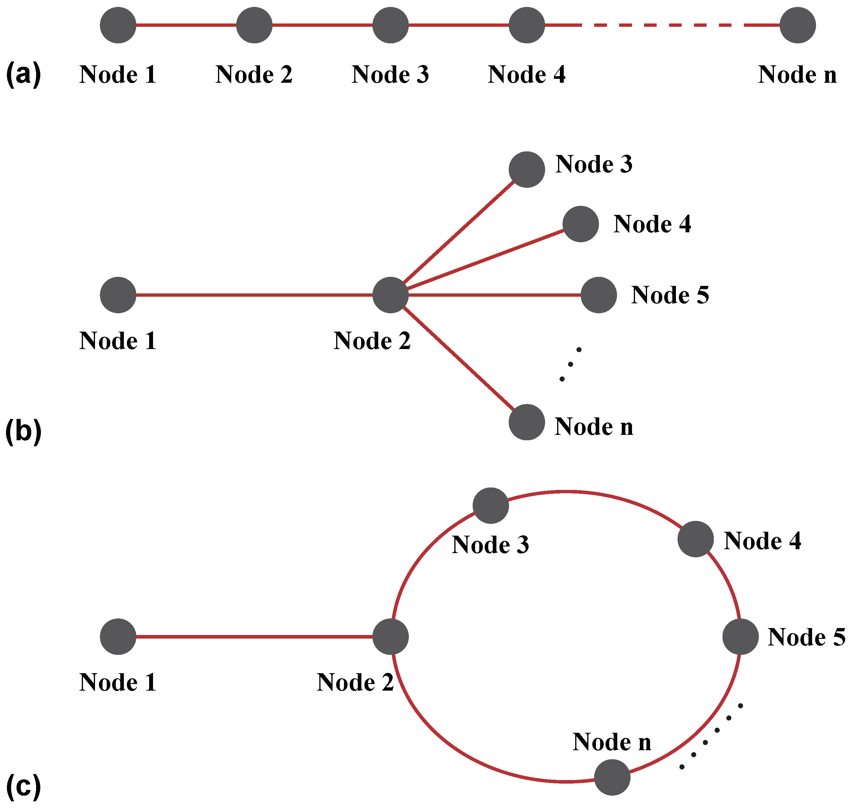
Some topologies for the interconnection of time synchronization networks are illustrated in Figure 1. Figure 1a illustrates a typical serial network structure, in which any intermediate node can divide the entire structure into two parts. The two parts can be regarded as two independent time synchronization networks, connected with each other via this node. This represents the most basic cascading structure of two networks. Figure 1b illustrates a tree-shaped time synchronization network formed by cascading a point-to-point system with a star-topology network. The point-to-point system between Node 1 and Node 2 can be regarded as the first stage of the entire system, while the star-topology network from Node 3 to Node n serves as the second stage. It can be considered that the two distinct networks are connected via Node 2. Similarly, a point-to-point system and a ring-topology network can also be cascaded to form a cascaded time synchronization network, as shown in Figure 1c. Multiple nodes in the ring network synchronize with Node 2 to form the second-stage time synchronization network, which is connected to the first-stage time synchronization network via Node 2. In summary, cascading is a common method employed for connecting different hierarchical levels in time synchronization networks. The flexible utilization of cascaded time synchronization systems enables the construction of relatively complex optical fiber time synchronization networks at a low cost, providing unified, high-precision time signals for multiple nodes over a wide area.

Figure 1. (a) Serial time synchronization networks structure formed by cascading two point-to-point systems. (b) Tree-shaped time synchronization networks formed by cascading a point-to-point system and a star-topology network. (c) Time synchronization networks formed by cascading a point-to-point system and a ring-topology network.

Furthermore, multiple time synchronization schemes can be employed in the same hierarchical level, and it should be carefully designed. One conventional approach is the cascading of multiple point-to-point systems, which has a relatively simple structure. However, since each subsequent stage relies on the preceding node as its timing reference, timing jitter propagate and accumulate along the cascade. To mitigate the accumulation of timing jitter, a common architecture is to insert couplers [30,31,32,33] or optical–electrical–optical (OEO) conversion modules [34] at intermediate nodes, so as to extract signals from the main link or facilitate signal transmission with other nodes. In this architecture, intermediate nodes can directly obtain signals from the reference node, thereby circumventing the timing jitter accumulation in cascaded chains. Alternatively, electrical regeneration and resynchronization modules deployed at the end nodes can further suppress jitter accumulation. In such configurations, the timing signal is regenerated locally, with its delay adjusted based on the measured clock offset. Consequently, the timing jitter of the regenerated signal is primarily governed by the module’s local frequency reference, whereas the time synchronization system contributes mainly to long-term stability without significantly affecting short-term jitter. In summary, diverse techniques are available to mitigate timing jitter within hierarchical networks. Although this paper focuses on inter-hierarchical connections in time synchronization networks, where cascading is the common viable architecture, the selection of an appropriate intra-hierarchical synchronization scheme is equally critical.

When designing fiber-optic time synchronization networks in a cascaded architecture, we identified two primary application scenarios. The first involves leveraging wide-area fiber infrastructure to transmit high-precision time and frequency signals across multiple regions, analogous to the backbone network in conventional optical communication systems. The second scenario utilizes metropolitan fiber resources to distribute synchronized clock signals within a city, similar to an access network. By integrating these two layers, high-precision time synchronization can be extended to multiple nodes, including both backbone and access nodes, over a broad geographical area. When integrating these two types of systems through cascaded networking, it is apparent that they operate under significantly different fiber link conditions. Backbone networks spanning multiple regions typically cover hundreds to thousands of kilometers, whereas metropolitan links—even in large cities such as Beijing—are generally under 100 km. Therefore, distinct system designs are essential for the backbone and metropolitan segments in fiber-based time–frequency synchronization networks.

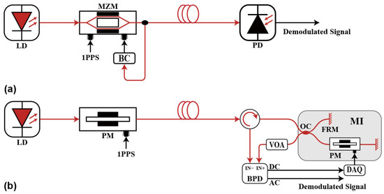
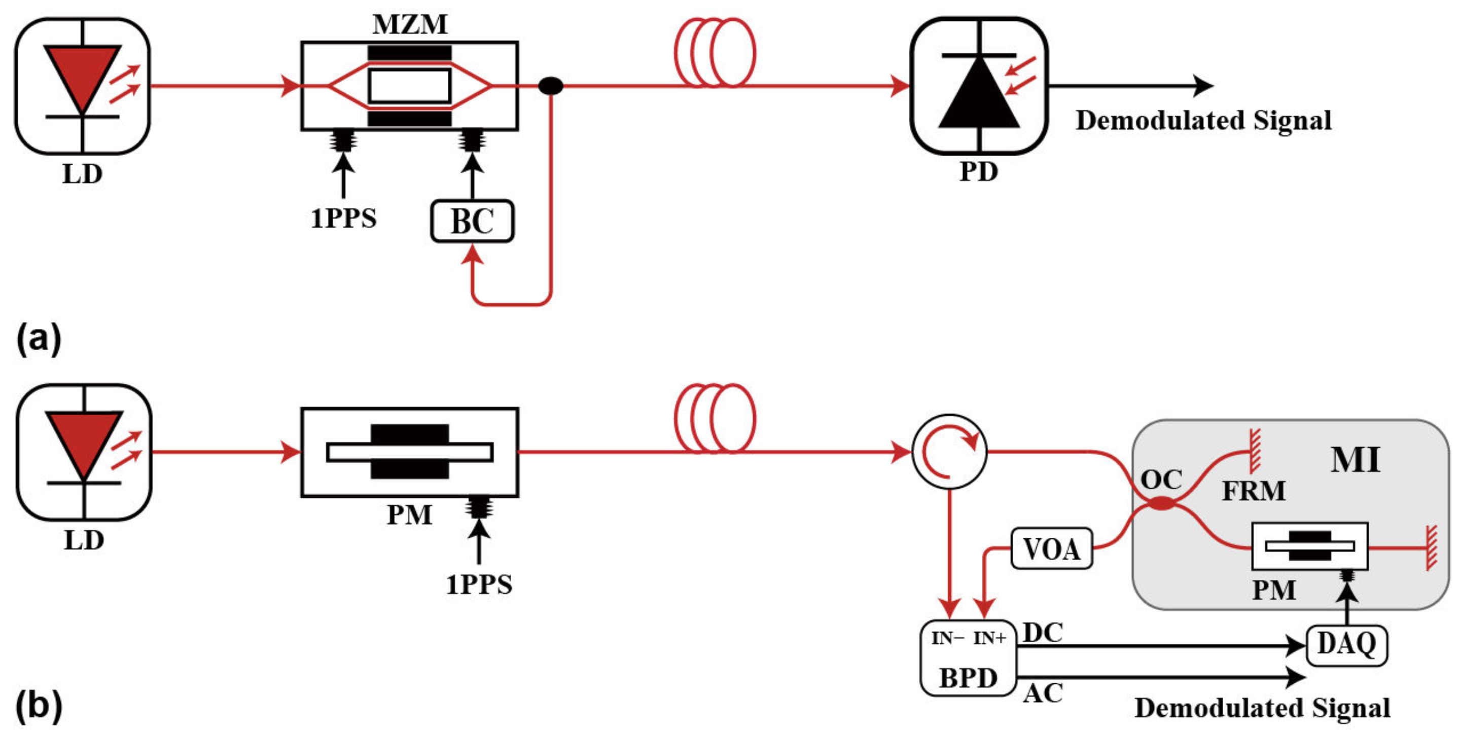
In the construction of fiber-optic time synchronization networks, analog one pulse per second (1PPS) is commonly used as the timestamp, with its rising edge serving as the trigger. Two primary modulation formats are employed: intensity modulation (IM) and phase modulation (PM), as illustrated in Figure 2. These two schemes differ in their operational principles and the required modulation/demodulation components. As shown in Figure 2a, the IM scheme has a simpler structure. In terms of devices, it only requires a Mach–Zehnder modulator (MZM) and a photodetector (PD) to accomplish signal modulation and detection. In some cases, the MZM can even be replaced by a directly modulated laser (DML) for a low-cost design [35]. However, high-performance 1PPS transmission under IM demands a high extinction ratio during modulation, which requires precise and stable bias control of the MZM [36]. In contrast, the PM scheme eliminates the need for bias control during modulation but involves greater complexity in demodulation. Since the signal is encoded in the optical phase, coherent detection is necessary [37]. Currently, delay self-interferometry-based demodulation is a mature approach, with an interferometer serving as the core component, as shown in Figure 2b. Although the PM scheme has complex demodulation and is limited by the laser linewidth, the signal light intensity remains unaffected by the modulated signal, enabling constant-envelope transmission. Thus, the difference between high extinction ratio signals and constant-envelope signals constitutes a significant distinction between the IM and PM schemes, and this difference can be analyzed from the nonlinear effect of fiber.

Figure 2. Comparison of signal modulation and demodulation schemes: (a) intensity modulation with direct detection (IMDD) scheme; (b) phase modulation with self-coherent detection (PMSCD) scheme. LD, laser diode; 1PPS, one pulse per second; BC, bias control; MZM, Mach–Zehnder modulator; PD, photodetector; PM, phase modulator; MI, Michelson interferometer; VOA, variable optical attenuator; OC, optical coupler; FRM, faraday rotation mirror; BPD, balanced photodetector; DC, direct current; AC, alternating current; and DAQ, data acquisition.

Considering single-channel transmission only, i.e., neglecting cross-phase modulation and four-wave mixing, the simplified form of the generalized nonlinear Schrödinger equation (NLSE) is given in Equation (1).

$${\displaystyle \frac{\partial U}{\partial z}}=-{\displaystyle \frac{\alpha }{2}}U+i{\displaystyle \frac{{\beta }_2}{2}}{\displaystyle \frac{{\partial }^{2}U}{\partial T^2}}+i\gamma {\left|U\right|}^{2}U.$$

(1)

In the NLSE, U denotes the complex envelope of the optical field, z represents the propagation distance, T indicates the time delay in a reference frame that moves along with the pulse group velocity, $\alpha$ represents the optical fiber attenuation coefficient, ${\beta }_2$ stands for the group velocity dispersion (GVD) coefficient, and $\gamma$ refers to the fiber nonlinear coefficient. Among them, the three corresponding components presented at the right side of the NLSE respectively represent the effects of fiber loss, fiber dispersion, and self-phase modulation (SPM). When $z=0$, the optical field and intensity of the signal light are given by: $U(0,T)=A\left(T\right) e^{i\psi }$, $I(0,T)={\left|U(0,T)\right|}^2=A^2\left(T\right)$.

When considering only the nonlinear effect of SPM and fiber attenuation, the optical field at z is given by:

$$\tilde{U}\left(z,T\right)=U\left(0,T\right)exp\left(-{\displaystyle \frac{\alpha }{2}}z\right)exp\left(i{\varphi }_{NL}\left(T\right)\right),$$

(2)

where ${\varphi }_{NL}\left(T\right)=\gamma L_{eff}\left(z\right)A^2\left(T\right)$, and $L_{eff}$ is the effective nonlinear interaction length, which characterizes the impact of attenuation on the accumulation of nonlinearity:

$$L_{eff}={\displaystyle \frac{1-exp\left(-\alpha z\right)}{\alpha }}.$$

(3)

SPM arises from the Kerr effect, which is the most prominent nonlinear effect in optical fibers. It describes how the intensity of the optical field itself affects the refractive index of the fiber, thereby influencing the phase of the optical field. Therefore, significant differences emerge in the optical field under the SPM effect when comparing high-extinction-ratio signals (i.e., IM-modulated signals) and constant-envelope signals (i.e., PM-modulated signals). For constant-envelope signals, the SPM-induced phase shift remains constant due to the stable signal intensity. In contrast, high-extinction-ratio signals exhibit substantial power fluctuations, resulting in unpredictable phase perturbations.

Building on Equation (2) and further considering fiber dispersion, the transmitted optical field can be expressed as Equation (4), where the dispersion propagation operator can be approximated by a power series in the time domain.

$$\begin{array}{cc}\hfill U\left(z,T\right)& =\tilde{U}\left(z,T\right)exp\left(i{\displaystyle \frac{{\beta }_{2}z}{2}}{\partial }_T^2\right)\hfill \\ \hfill & \approx \tilde{U}\left(z,T\right)+i{\displaystyle \frac{{\beta }_{2}z}{2}}{\partial }_T^2\tilde{U}\left(z,T\right).\hfill \end{array}$$

(4)

Therefore, the intensity of the signal light can be approximated as:

$$\begin{array}{cc}\hfill I\left(z,T\right)& ={\left|U\left(z,T\right)\right|}^2\hfill \\ \hfill & \approx {\left|\tilde{U}\left(z,T\right)\right|}^2+{\beta }_{2}zIm\left\{{\tilde{U}}^{*}\left(z,T\right){\partial }_T^2\tilde{U}\left(z,T\right)\right\}.\hfill \end{array}$$

(5)

Substituting Equation (2) into Equation (5) and simplifying, the following Equation (6) can be obtained:

$$\begin{array}{cc}\hfill I\left(z,T\right)\approx & A^2\left(T\right)exp\left(-\alpha z\right)\hfill \\ & +{\beta }_{2}zA\left(T\right)\left(2A^{\prime }\left(T\right){\varphi }_{NL}^{\prime }\left(T\right)+A\left(T\right) {\varphi }_{NL}^{\prime \prime }\left(T\right)\right).\hfill \end{array}$$

(6)

And Equation (6) can be further rearranged as:

$$\begin{array}{cc}\hfill I\left(z,T\right)\approx & I\left(0,T\right)exp\left(-\alpha z\right)\hfill \\ & +\gamma {\beta }_2{L}_{eff}z\left({\left(I^{\prime }\left(T\right)\right)}^2+I\left(T\right) I^{″}\left(T\right)\right).\hfill \end{array}$$

(7)

Equation (7) indicates that for intensity time-varying light, the phase perturbation induced by SPM is converted into amplitude perturbation via fiber dispersion. Moreover, this perturbation depends strongly on the first and second time derivatives of the optical intensity. Consequently, under the combined influence of SPM and dispersion, temporal distortion of the signal manifests predominantly at the rising and falling edges. This is particularly detrimental in rising-edge-triggered fiber-optic time synchronization systems, where such distortions can significantly degrade performance.

To quantitatively elucidate the impact of SPM and dispersion on IMDD time synchronization performance, comprehensive numerical simulations were performed. The waveform of the timing signal is a double Sigmoid pulse. The timing signal is given by:

$$\begin{array}{c}\hfill V\left(T\right)=V_0[{\displaystyle \frac{1}{1+exp(-\frac{T+\frac{T_{pw}}{2}}{T_r})}}-{\displaystyle \frac{1}{1+exp(-\frac{T-\frac{T_{pw}}{2}}{T_r})}}].\end{array}$$

(8)

where $T_{pw}$ is the pulse width, $T_r$ is the rise time, and $V_0$ is the pulse amplitude.

Intensity modulation is performed using an ideal Mach–Zehnder modulator (MZM), which is biased at the null point. Therefore, A(T) is given by:

$$\begin{array}{c}\hfill A\left(T\right)=A_{0}sin[{\displaystyle \frac{\pi V\left(T\right)}{2V_{\pi }}}]\end{array}$$

(9)

where $A_0$ is the amplitude of $A\left(T\right)$, and $V_{\pi }$ is the half-wave voltage of the modulator. The modulation depth is set to 1, i.e., $V_0=V_{\pi }$. Substituting Equation (8) into Equation (9) and simplifying, $I(0,T)$ can be obtained:

$$\begin{array}{c}\hfill I(0,T)=A^2\left(T\right)={\displaystyle \frac{A_0^2}{2}}\left\{1-cos\left[{\displaystyle \frac{\pi }{1+exp(-\frac{T+\frac{T_{pw}}{2}}{T_r})}}-{\displaystyle \frac{\pi }{1+exp(-\frac{T-\frac{T_{pw}}{2}}{T_r})}}\right]\right\}.\end{array}$$

(10)

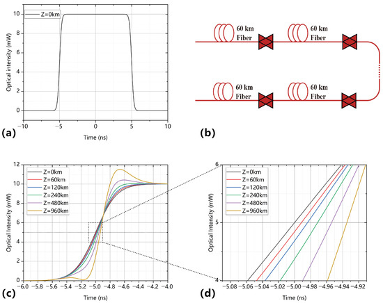
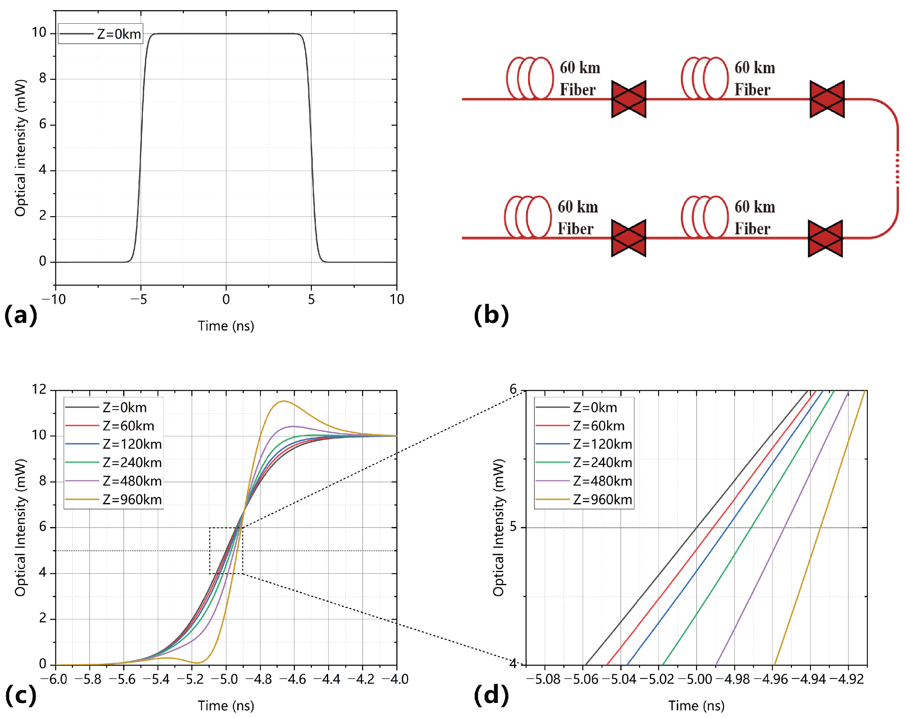
For a pulse width of $T_{pw}=10$ ns, a rise time of $T_r=1$ ns, and a peak power of $A_0^2=10$ mW, the optical signal waveform at $Z=0$ is illustrated in Figure 3a. The optical signal propagates along the fiber link shown in Figure 3b, which employs a standard single-mode fiber with the fiber attenuation coefficient $\alpha =0.2$ dB/km, the group velocity dispersion coefficient ${\beta }_2=-20$ ps²/km, and the nonlinear coefficient $\gamma =1.3$ W⁻¹km⁻¹. Ideal optical amplifiers with negligible noise are placed at 60 km intervals to fully compensate for fiber loss and restore the signal to its launched power $I(0,T)$. The rising-edge waveforms of the optical signal after transmission are shown in Figure 3c. In the construction of fiber-optic time synchronization networks, analog one pulse per second (1PPS) is commonly used as the timestamp, with its rising edge serving as the trigger. In time synchronization systems, the mid-amplitude point of the 1PPS signal’s rising edge is commonly used as the trigger. Accordingly, the corresponding positions are magnified and shown in Figure 3d. It can be observed that as the transmission distance increases, the waveform distortion of the optical signal becomes more severe, and the trigger timing error gradually increases. The trigger timing error is 8.6 ps at a transmission distance of 60 km, and increases to 65.3 ps when the distance reaches 960 km in our simulation.

Figure 3. (a) The optical signal waveform at $Z=0$. (b) The ideal fiber-optic link established in the simulation. (c) The rising-edge waveforms of the optical signal after transmission. (d) Magnified view of the mid-amplitude point of the optical signal’s rising edge.

It should be noted that the aforementioned simulations represent theoretical analyses under idealized conditions. In practical deployments, fiber link parameters are subject to environmental perturbations. For example, group velocity dispersion coefficient ${\beta }_2$, nonlinear coefficient $\gamma$ and transmission distance Z are sensitive to temperature variations. In addition, gain fluctuations of optical amplifiers will change the effective nonlinear interaction length $L_{eff}$. As waveform distortion and trigger timing error intensify with propagation distance, the resulting timing error variation under environmental disturbances expands correspondingly, severely compromising time synchronization stability.

For IMDD time synchronization systems, the combined effects of SPM and dispersion lead to signal distortion, thereby generating trigger timing offset and jitter. Such influence accumulates as the transmission distance increases. When the distance reaches hundreds of kilometers, the timing error can reach tens of picoseconds, which evidently deteriorates the accuracy and long-term stability of time synchronization performance.

In contrast, PMSCD systems maintain constant optical power, rendering SPM-induced distortion negligible. Consequently, PMSCD systems are more suitable for long-haul transmission than their IMDD systems.

Therefore, in the cascaded fiber-optic time synchronization network that we have designed, even though the IMDD system is more cost-effective, it can only be used as a short-distance distribution system. In contrast, the PMSCD system, which exhibits significant advantages in long-distance fiber-optic link transmission, should be employed as the system for the backbone fiber link.

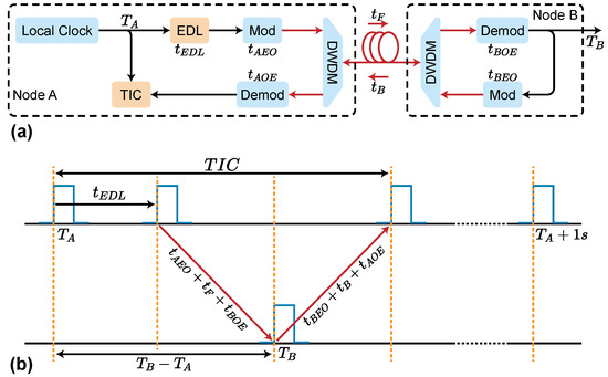
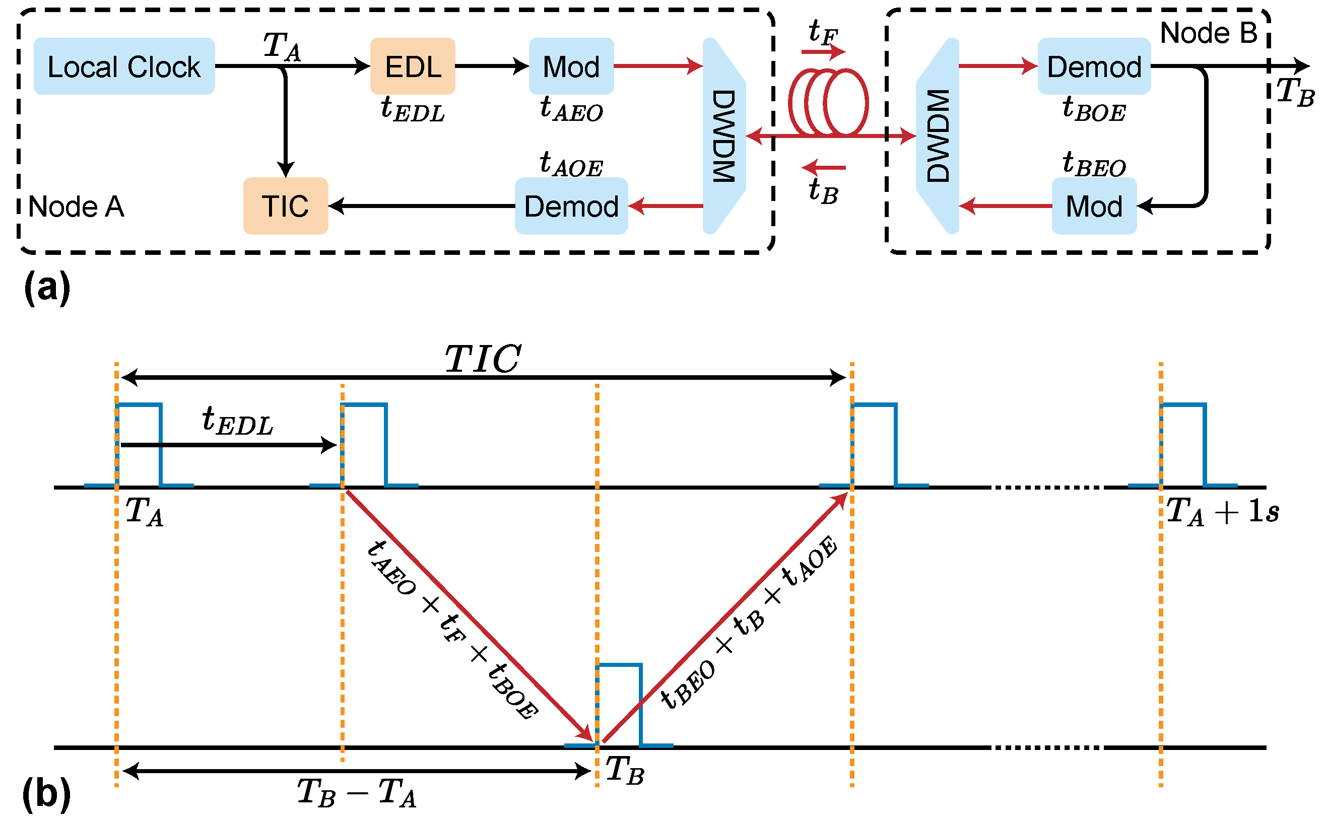
The cascaded time synchronization system we designed utilizes a round-trip time synchronization scheme, whose basic configuration and timing model are illustrated in Figure 4. In this scheme, a time interval counter (TIC) is adopted to acquire the round-trip transmission delay of optical signals. Leveraging the reciprocity of bidirectional transmission delays, the one-way delay between two nodes is calculated and compensated via an electronic delay line (EDL). This architecture is relatively simple and capable of achieving picosecond-level synchronization accuracy. Furthermore, since both delay measurement and compensation are performed locally without requiring data transmission to a remote site, the scheme offers high feasibility for practical engineering applications.

Figure 4. (a) The basic structure of round-trip time synchronization system. (b) The timing model of the round-trip system. EDL, electronic delay line; TIC, time interval counter; Mod, modulation module; Demod, demodulation module; and DWDM, dense wavelength-division multiplexer. $T_A$ and $T_B$ stand for the timestamp at node A and B; $t_{EDL}$ denotes the delay introduced by the EDL; $t_{AOE}$ ($t_{AEO}$) represents the electro-optic (photoelectric) conversion delay at node A; $t_F$ ($t_B$) is the forward (backward) transmission delay of the fiber link; and $t_{BOE}$ ($t_{BEO}$) is the electro-optic (photoelectric) conversion delay in node B.

According to the timing model of round-trip time synchronization system, the round-trip delay measured by TIC at node A can be expressed as

$$TIC=t_{EDL}+t_{AEO}+t_F+t_{BOE}+t_{BEO}+t_B+t_{AOE}.$$

(11)

And the clock difference between two nodes is

$$\mathrm{\Delta }T=T_B-T_A=t_{EDL}+t_{AEO}+t_F+t_{BOE}.$$

(12)

Given that the delay caused by the EDL is known and the system asymmetry is considered, the time offset between the two nodes can be derived as

$$\begin{array}{cc}\hfill \mathrm{\Delta }T=& {\displaystyle \frac{TIC+t_{EDL}}{2}}\hfill \\ \hfill & +{\displaystyle \frac{\left(t_{AEO}+t_F+t_{BOE}\right)-\left(t_{BEO}+t_B+t_{AOE}\right)}{2}}.\hfill \end{array}$$

(13)

The second term in Equation (13) is the system asymmetry and represents inconsistencies in the delay of bidirectional transmissions. The total system asymmetry can be decomposed into two components: asymmetry introduced by the transceiver devices and asymmetry caused by the optical fiber links. Transceiver device asymmetry is determined via back-to-back calibration experiments. Fiber link asymmetry is characterized using a self-developed test platform [38], which enables the calibration of bidirectional optical amplifier asymmetry and the measurement of fiber link dispersion.

In Equation (13), both the TIC and EDL-induced delay are known quantities. The asymmetric component can also be accurately determined through calibration. Consequently, the time offset of the time synchronization system constitutes a determinate, precisely measurable quantity that can be effectively compensated using established techniques such as phase-locked regeneration or programmable delay modules.

In the designed cascaded time synchronization system, synchronization between nodes A and B is achieved using the round-trip scheme. Meanwhile, nodes B and C operate an independent round-trip system based on the synchronized 1PPS signal at node B. Therefore, the two subsystems involving three nodes operate independently and do not interfere with each other. Under this configuration, the timing jitter at node C relative to node A corresponds to the superposition of the jitter contributions from both subsystems [39], that is,

$${\sigma }_{CA}=\sqrt{{\sigma }_{CB}^2+{\sigma }_{BA}^2},$$

(14)

where ${\sigma }_{BA}$ is the jitter of the first subsystem between nodes A and B, and ${\sigma }_{CB}$ is similarly defined as the jitter of the second subsystem between nodes B and C.

3. Experiment Setup and Results

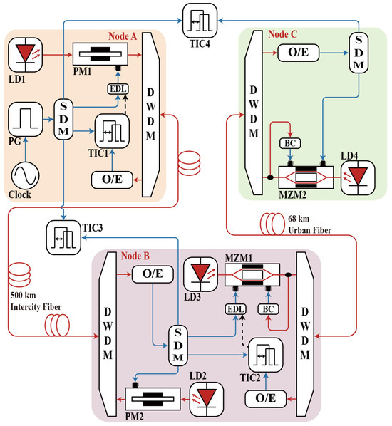
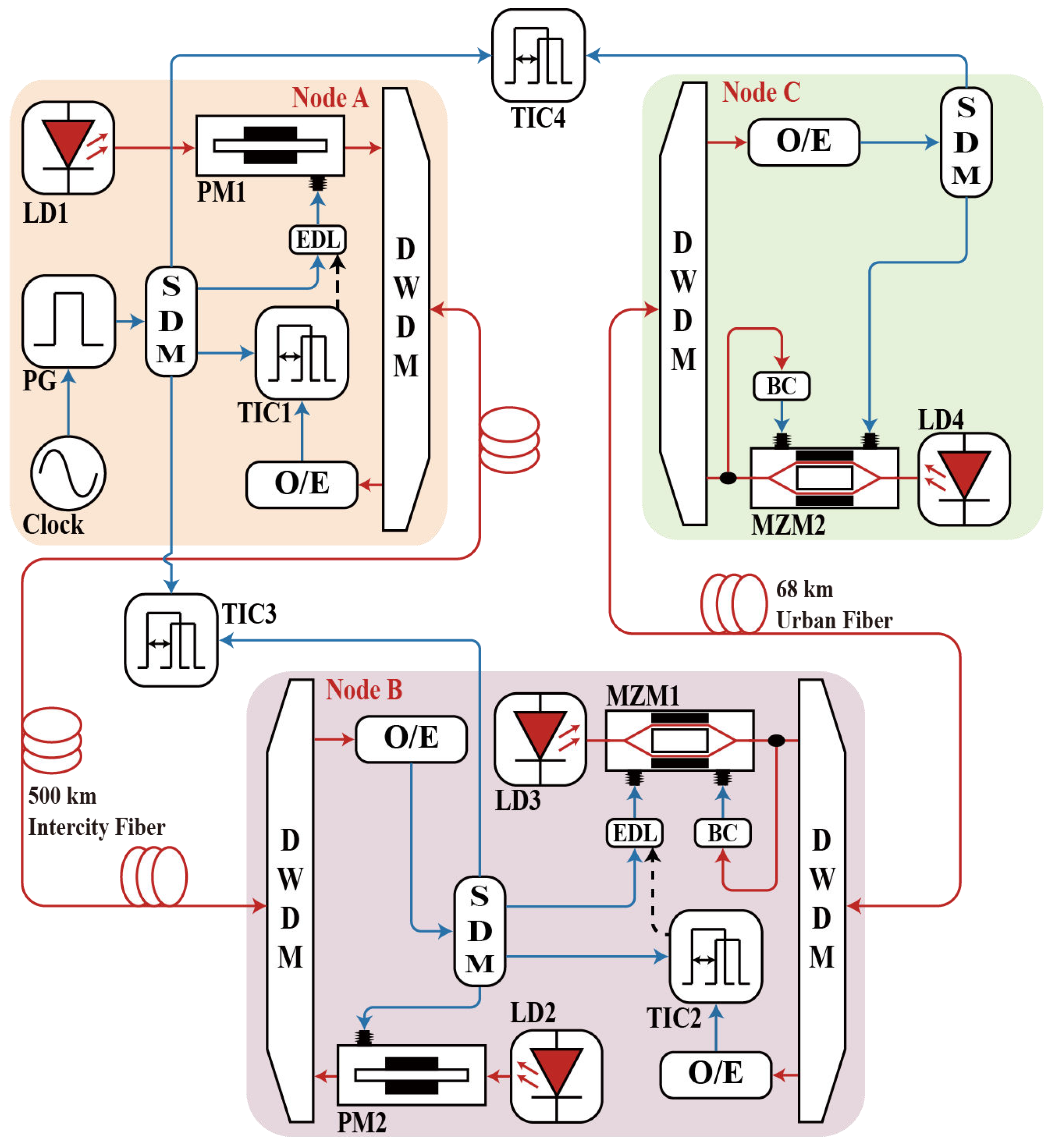
Based on the above analysis, we have designed and implemented a cascaded time synchronization system that employs a hybrid IM/PM modulation scheme to synchronize three nodes (A, B, and C), and validated its performance through experiments over real-world fiber links. The experimental setup is illustrated in Figure 5. In node A, the pulse generator (PG, Stanford Research Systems DG645), driven by the high-stability 10 MHz reference signal from Rb atomic clock, generates a 1PPS signal synchronized with the clock, and the 1PPS signal is divided into multi-output by the signal distribution module (SDM). One of the outputs of the SDM connects with the phase modulator through an electric delay line (EDL). The whole system is a dense wavelength-division multiplexing (DWDM) system, in which the lasers have different wavelengths (${\lambda }_{LD1}={\lambda }_{LD3}=1551.72$ nm, and ${\lambda }_{LD2}={\lambda }_{LD4}=1550.12$ nm). In Node B, the 1PPS signal is demodulated by an O/E module comprising a Michelson interferometer (MI) and a balanced photodetector (BPD), the structure of which is identical to that shown in Figure 2b. The 1PPS output from the BPD is divided into four ports by the SDM. One of these connects to phase modulator 2 and transfers back to node A. So, that time interval between backward transmission 1PPS and local 1PPS can be measured by time interval counter 1 (TIC1, Keysight 53230A). The EDL is used to compensate the fiber transmission delay according to the measurement results of TIC 1. Subsystem 2 operates in the same manner. There are two main differences between the two subsystems: First, the reference 1PPS of subsystem 2 comes from the output of subsystem 1, and the measurement of the round-trip delay and the compensation of the transmission delay are completed at node B, primarily implemented by TIC 2 and EDL. Second, subsystem 2 operates in the IMDD modulation format, with the modulating device being an MZM and the demodulating device being a PD, without the need to pass through MI, which makes the structure of subsystem 2 simpler than that of subsystem 1. To assess the timing synchronization accuracy of the whole cascaded system, all three nodes are placed in the same laboratory. TIC 3 is used to assess the time synchronization precision between nodes A and B, while TIC 4 is employed to evaluate the time synchronization precision between nodes A and C.

Figure 5. The experimental setup for the proposed cascaded fiber-optic time synchronization system, which uses both IM and PM modulation formats. LD, laser diode; PM, phase modulator; PG, pulse generator; SDM, signal distribution module; EDL, electronic delay line; O/E, optoelectronic conversion; DWDM, dense wavelength-division multiplexer; MZM, Mach–Zehnder modulator; BC, bias control; and TIC, Time Interval Counter.

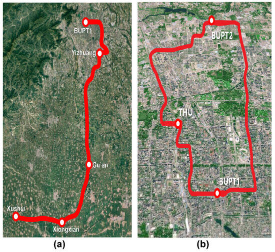
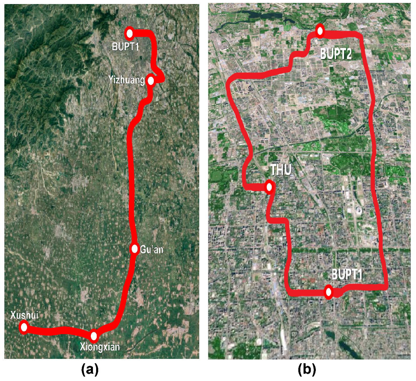
Two real-world fiber links are employed in this experiment, as shown in Figure 6. The first is an intercity link connecting Beijing and Baoding, Hebei Province. Subsystem 1 was established over this link. The link originates at the Xitucheng Campus of Beijing University of Posts and Telecommunications (BUPT 1) and terminates at a fiber access facility in Xushui District, Baoding, passing through three intermediate sites: Yizhuang (Beijing), Gu’an (Hebei), and Xiongxian (Hebei). Two fiber cores within this link were utilized. One core carried the 1PPS signal from BUPT 1 to Xushui. At Xushui, an erbium-doped fiber amplifier (EDFA) amplified the received optical signal, which was then returned via the second core to BUPT 1. As a result, both nodes A and B of subsystem 1 are co-located in the same laboratory at BUPT 1. To compensate for fiber attenuation, two bidirectional EDFAs were deployed at each of the three intermediate sites: Yizhuang, Gu’an, and Xiongxian. Therefore, the total fiber length is approximately 500 km. The length of this link is essentially equivalent to the possible distance between two cities, approximately 1.5 times the distance between Shanghai and Nanjing. Therefore, we used this link to simulate the intercity transmission scenario of a fiber-optic time synchronization system. According to the aforementioned analysis, the PMSCD system, due to its constant-envelope characteristic, is less susceptible to self-phase modulation caused by the Kerr effect in the fiber link, and thus is considered to have better noise resistance. Consequently, we established a PMSCD system as subsystem 1 over this 500 km long intercity fiber link. The second fiber link forms a loop within Beijing, starting from and returning to the BUPT 1 laboratory after encircling the city. This segment also passes through the Hongfu Campus of Beijing University of Posts and Telecommunications (BUPT 2) and Tsinghua University, with a total length of 68 km. Given the relatively short distance, nonlinear effects remain manageable. We therefore implemented an IMDD system as subsystem 2 over this link. The loop configuration co-locates nodes B and C of subsystem 2 within the same laboratory, simplifying subsequent evaluation.

Figure 6. The fiber links employed in this experiment: (a) the 500 km intercity fiber link from Beijing to Xushui in Hebei Province; (b) the 68 km loop fiber link within Beijing.

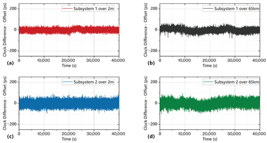
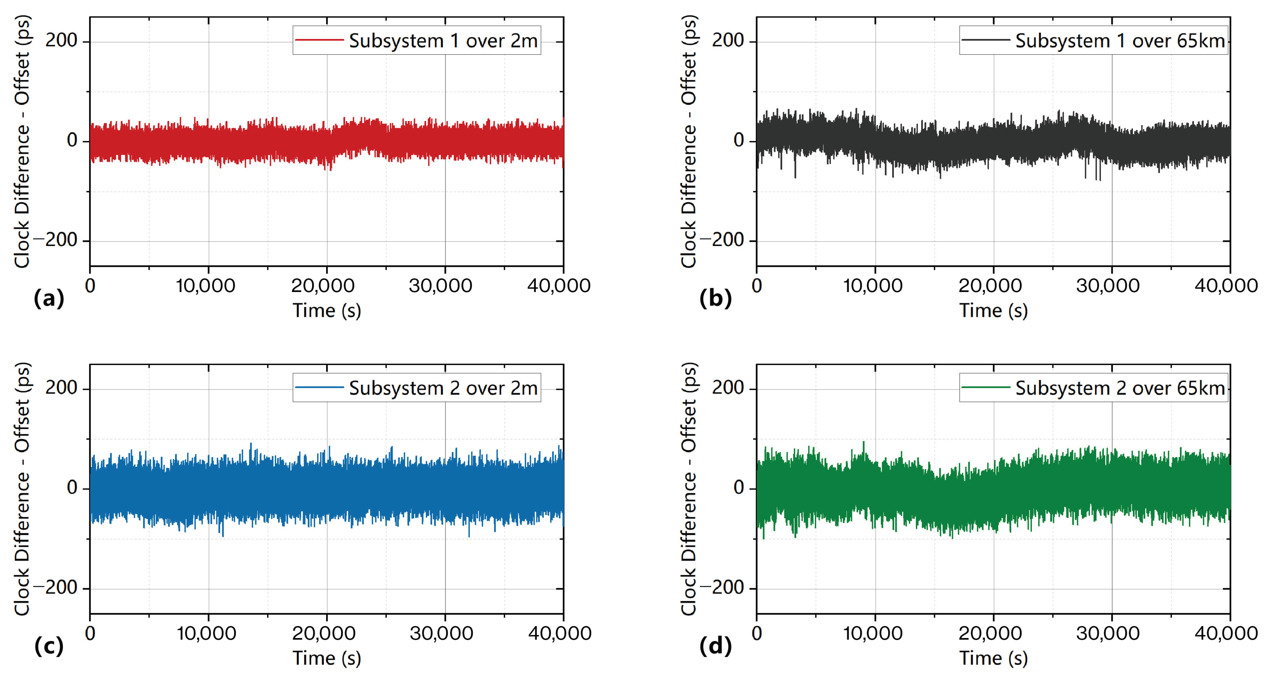
To evaluate the performance of the two subsystems, we first performed comparative tests on both subsystems in the laboratory. The two subsystems were operated independently over the identical 2 m short optical fiber and the laboratory 65 km optical fiber link, with the test results shown in Figure 7. For direct comparison, the measured data have been corrected for the corresponding system time offset and are presented on a unified time scale. All tests lasted for more than 40,000 s, and the measured results were stable with no significant fluctuations. The timing jitter of Subsystem 1 was 13.29 ps in the back-to-back experiment and 17.44 ps in the 65 km transmission experiment. For Subsystem 2, the timing jitter was 22.85 ps in the back-to-back experiment and 26.66 ps in the 65 km transmission experiment. These results confirm that Subsystem 1 achieves superior performance relative to Subsystem 2 in terms of both inherent noise floor and transmission-induced timing jitter.

Figure 7. (a) The measured clock difference of subsystem 1 over 2 m fiber. (b) The measured clock difference of subsystem 1 over a 65 km fiber link. (c) The measured clock difference of subsystem 2 over 2 m fiber. (d) The measured clock difference of subsystem 2 over a 65 km fiber link.

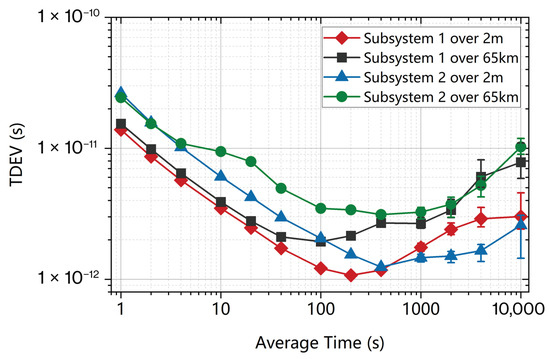
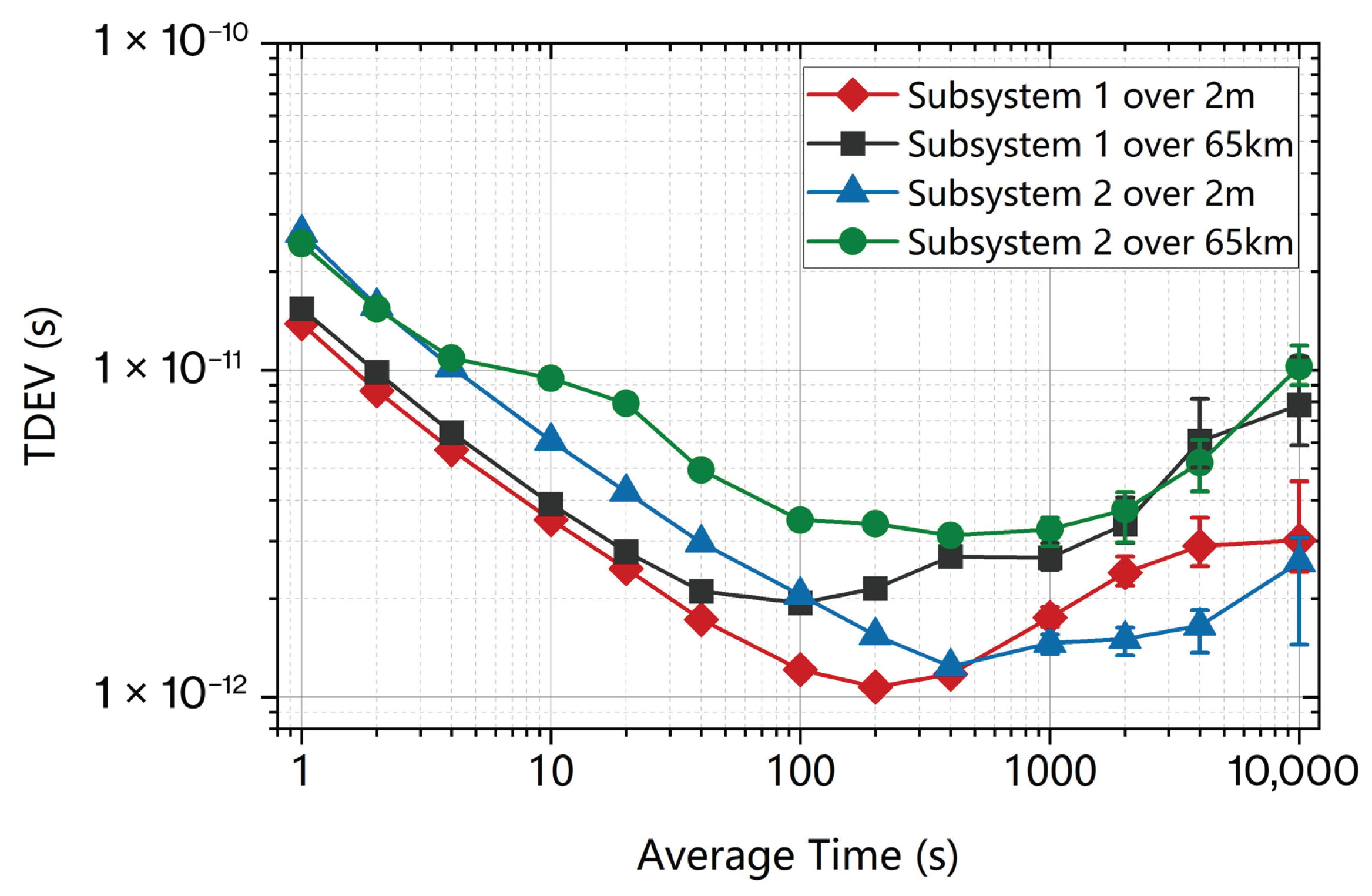
We also compared the time deviation (TDEV) of the experimental results, as shown in Figure 8. For the back-to-back synchronization, the time synchronization stability of subsystem 1 (red curve) is 13.9 ps at 1 s and 3.0 ps at 10,000 s, decreasing continuously with averaging time to reach a minimum at $\tau =200$ s before diverging. The time synchronization stability of subsystem 2 (blue curve) is 26.3 ps at 1 s and 2.6 ps at 10,000 s. While its long-term performance is consistent with that of subsystem 1, its short-term stability is significantly degraded by comparison. For the 65 km fiber transmission experiments, the time synchronization stability of subsystem 1 (black curve) is 15.4 ps at 1 s and 7.8 ps at 10,000 s. Its short-term stability is essentially consistent with the noise floor, while its long-term stability deteriorates due to environmental fluctuations, such as variations in fiber length and laser wavelength drift. The time synchronization stability of subsystem 2 (green curve) is 24.3 ps at 1 s and 10.3 ps at 10,000 s. Its short-term performance is consistent with the back-to-back baseline, while its long-term stability demonstrates excellent consistency with subsystem 1 under the 65 km fiber transmission.

Figure 8. The TDEV curves for laboratory comparative tests: the measured clock difference of subsystem 1 over 2 m fiber; the measured clock difference of subsystem 1 over a 65 km fiber link; the measured clock difference of subsystem 2 over 2 m fiber; and the measured clock difference of subsystem 2 over a 65 km fiber link.

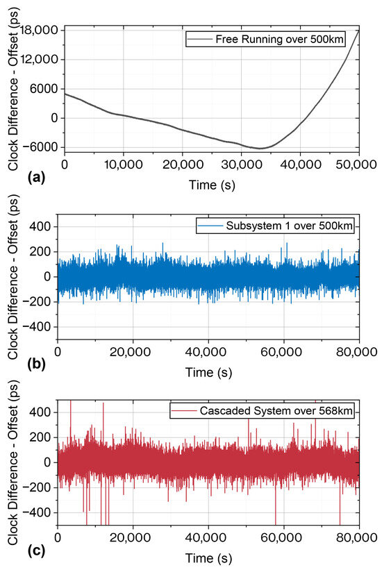
Based on the aforementioned experimental and fiber-optic link configurations, we conducted multiple tests, as shown in Figure 9. Initially, we measured the free-running fiber transmission delay in the 500 km intercity fiber link, as depicted in Figure 9a. In this test, the EDL in subsystem 1 did not compensate for the fiber transmission delay drift, and the delay between nodes A and B was directly measured by TIC 3. It is evident that, without compensation, the fiber transmission delay experiences significant drift, with an amplitude exceeding 24 ns. Subsequently, the EDL in subsystem 1 was activated to compensate for the fiber transmission delay, as determined by the TIC 1 measurement results. The clock difference between two nodes was reassessed using TIC 3, yielding the results shown in Figure 9b. A comparison of Figure 9a and Figure 9b reveals that, after compensation was initiated, the drift in fiber transmission delay was effectively suppressed and subsystem 1 remained stable throughout the test period, which lasted slightly less than one day. Over the 80,000 s test duration, the time synchronization jitter of subsystem 1 was 40.97 ps. With subsystem 1 functioning properly, we then activated subsystem 2 and validated the time synchronization results of the cascaded system using TIC 4, as illustrated in Figure 9c. It is apparent that the cascaded system also remained stable over the 80,000 s measurement period without any noticeable drift. However, due to the superposition of jitter from the two subsystems, the cascaded system exhibited slightly higher jitter than subsystem 1, with a value of 48.87 ps. Although the jitter between nodes B and C was not directly assessed, we can calculate that the jitter of subsystem 2 is approximately 26.64 ps using the relationship given in Equation (14). This theoretical result is highly consistent with the experimental value of 26.66 ps measured over a 65 km laboratory link, confirming the validity of the synthesis approach. As the transmission distance of subsystem 2 is only about one-seventh of that of subsystem 1, its jitter performance cannot be considered ideal.

Figure 9. (a) The measured free-running clock difference over a 500 km intercity fiber link. (b) The measured clock difference over a 500 km intercity fiber link with fiber transmission delay compensation. (c) The measured clock difference over a 568 km metropolitan fiber link with fiber transmission delay compensation.

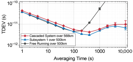
We also compared the time deviation (TDEV) of the three sets of data, as shown in Figure 10. For the two sets of data acquired from the 500 km intercity optical fiber link, TDEV profiles present excellent consistency when the averaging time ranges from 1 s to 100 s. However, the stability degrades for averaging times exceeding 100 s due to the obvious delay drift experienced by the free-running data. In contrast, with delay compensation activated, a slight degradation occurs only when the averaging time exceeds 400 s. For subsystem 1 operating over the 500 km intercity fiber-optic link, the time synchronization stability is 37.8 ps at the averaging time of 1 s and 6.7 ps at 10,000 s. As indicated by the red curve in Figure 10, the trend of the cascaded system data is highly similar to that of the blue curve representing the stability of subsystem 1. This is due to the longer transmission distance of subsystem 1, which dominates the stability when the two subsystems are cascaded. The time synchronization stability of the cascaded system is 43.9 ps at 1 s and 9.8 ps at 10,000 s.

Figure 10. The TDEV curves for three different conditions: the measured free-running clock difference over a 500 km intercity fiber link; the measured clock difference over a 500 km intercity fiber link with fiber transmission delay compensation; and the measured clock difference over a 568 km metropolitan fiber link with fiber transmission delay compensation.

4. Discussion

Based on the nonlinear Schrödinger equation (NLSE), we analyze the effects of self-phase modulation (SPM) and chromatic dispersion on optical signals. The results indicate that waveform distortion occurs for time-varying optical power signals after fiber transmission. The distortion degree is closely related to the first and second time derivatives of optical power. Sharper temporal changes in optical power will result in more severe signal distortion. Besides, signal distortion accumulates continuously, and becomes more serious as the transmission distance increases.

Numerical simulations are carried out to analyze the influence of such signal distortion on time synchronization systems. The results show that waveform distortion will induce timing trigger errors at the receiving terminal. Typically, after hundreds-of-kilometer fiber transmission, the degradation of time synchronization accuracy caused by signal distortion can reach tens of picoseconds.

By comparing the theoretical analysis with simulation results, we argue that IMDD systems possess no inherent advantages for long-distance fiber-optic time synchronization, whereas PMSCD systems benefit from the fact that modulation signals do not induce optical power variations, which makes SPM-induced distortion negligible.

5. Conclusions

To achieve a fiber-optic time synchronization network with broad geographical applicability, we conducted experimental validations over real-world fiber links connecting Beijing and Hebei, as well as within Beijing. For the system design, we evaluated two modulation formats: IMDD and PMSCD. Based on a comparative analysis of their respective advantages and limitations, we adopted the PMSCD system for long-haul intercity time signal transmission and the IMDD system for metropolitan-area time signal distribution. Following this approach, we implemented a two-stage cascaded fiber-optic time synchronization system over a total link length of 568 km. The overall timing precision was maintained within 50 ps, underscoring the practical utility of the proposed architecture and offering a valuable engineering reference for future large-scale ground-based fiber-optic time and frequency networks.

References

- Levine, J. Introduction to time and frequency metrology. Rev. Sci. Instrum. 1999, 70, 2567–2596. [Google Scholar] [CrossRef] [Scilit]
- Droste, S.; Udem, T.; Holzwarth, R.; Haensch, T.W. Optical frequency dissemination for metrology applications. Comptes Rendus Phys. 2015, 16, 524–530. [Google Scholar] [CrossRef] [Scilit]
- Lopez, O.; Kéfélian, F.; Jiang, H.; Haboucha, A.; Bercy, A.; Stefani, F.; Chanteau, B.; Kanj, A.; Rovera, D.; Achkar, J.; et al. Frequency and time transfer for metrology and beyond using telecommunication network fibres. Comptes Rendus Phys. 2015, 16, 531–539. [Google Scholar] [CrossRef] [Scilit]
- Dow, J.M.; Neilan, R.E.; Rizos, C. The international GNSS service in a changing landscape of global navigation satellite systems. J. Geod. 2009, 83, 191–198. [Google Scholar] [CrossRef] [Scilit]
- Lewandowski, W.; Arias, E. GNSS times and UTC. Metrologia 2011, 48, S219–S224. [Google Scholar] [CrossRef] [Scilit]
- Li, X.; Ge, M.; Dai, X.; Ren, X.; Fritsche, M.; Wickert, J.; Schuh, H. Accuracy and reliability of multi-GNSS real-time precise positioning: GPS, GLONASS, BeiDou, and Galileo. J. Geod. 2015, 89, 607–635. [Google Scholar] [CrossRef] [Scilit]
- Delva, P.; Lodewyck, J.; Bilicki, S.; Bookjans, E.; Vallet, G.; Le Targat, R.; Pottie, P.-E.; Guerlin, C.; Meynadier, F.; Le Poncin-Lafitte, C.; et al. Test of special relativity using a fiber network of optical clocks. Phys. Rev. Lett. 2017, 118, 221102. [Google Scholar] [CrossRef] [Scilit] [PubMed]
- Boulder Atomic Clock Optical Network (BACON) Collaboration. Frequency ratio measurements at 18-digit accuracy using an optical clock network. Nature 2021, 591, 564–569. [Google Scholar] [CrossRef] [Scilit]
- Marra, G.; Clivati, C.; Luckett, R.; Tampellini, A.; Kronjäger, J.; Wright, L.; Mura, A.; Levi, F.; Robinson, S.; Xuereb, A.; et al. Ultrastable laser interferometry for earthquake detection with terrestrial and submarine cables. Science 2018, 361, 486–490. [Google Scholar] [CrossRef] [Scilit]
- Mehlstäubler, T.E.; Grosche, G.; Lisdat, C.; Schmidt, P.O.; Denker, H. Atomic clocks for geodesy. Rep. Prog. Phys. 2018, 81, 064401. [Google Scholar] [CrossRef] [Scilit]
- Yang, Y.; Ren, X.; Jia, X.; Sun, B. Development trends of the national secure PNT system based on BDS. Sci. China Earth Sci. 2023, 66, 929–938. [Google Scholar] [CrossRef] [Scilit]
- Langley, R.B.; Teunissen, P.J.; Montenbruck, O. Introduction to GNSS. In Springer Handbook of Global Navigation Satellite Systems; Springer: Berlin/Heidelberg, Germany, 2017; pp. 3–23. [Google Scholar]
- Piester, D.; Fujieda, M.; Rost, M.; Bauch, A. Time transfer through optical fibers (TTTOF): First results of calibrated clock comparisons. In Proceedings of the 41st Annual Precise Time and Time Interval Systems and Applications Meeting; The Institute of Navigation, Inc.: Manassas, VA, USA, 2009; pp. 89–100. [Google Scholar]
- Rost, M.; Piester, D.; Yang, W.; Feldmann, T.; Wübbena, T.; Bauch, A. Time transfer through optical fibres over a distance of 73 km with an uncertainty below 100 ps. Metrologia 2012, 49, 772. [Google Scholar] [CrossRef] [Scilit]
- Lopez, O.; Kanj, A.; Pottie, P.-E.; Rovera, D.; Achkar, J.; Chardonnet, C.; Amy-Klein, A.; Santarelli, G. Simultaneous remote transfer of accurate timing and optical frequency over a public fiber network. Appl. Phys. B 2013, 110, 3–6. [Google Scholar] [CrossRef] [Scilit]
- Zhang, C.; Li, Y.; Chen, X.; Zhang, Y.; Fu, L.; Gong, Y.; Wang, H.; Huang, W.; Xu, B. Controllable asymmetry attack on two-way fiber time synchronization system. IEEE Photonics J. 2021, 13, 3100106. [Google Scholar] [CrossRef] [Scilit]
- Wu, R.; Yang, F.; Sun, Y.; Wei, F.; Gui, Y.; Ding, Y.; Cai, H. Absolutely consistent fiber-optic phase synchronization based on fixed-phase-reference optical active compensation. IEEE Photonics J. 2021, 13, 7200311. [Google Scholar] [CrossRef] [Scilit]
- VanArsdale, J.; Deutch, M.J.; Lombardi, M.A.; Nelson, G.; Sherman, J.; Spicer, J.; Yates, W.; Yost, D.; Brewer, S. Dissemination of UTC (NIST) over 20 km of commercial optical fiber with active phase stabilization. Opt. Lett. 2024, 49, 2545–2548. [Google Scholar] [CrossRef] [Scilit]
- Cheng, J.; Wang, Z.; Qiao, Y.; Gao, H.; Liu, C.; Zhao, Z.; Zhang, J.; Zhao, B.; Luo, B.; Yu, S. A CNN-LSTM phase compensation method for unidirectional two-way radio frequency transmission system. IEEE Photonics J. 2024, 16, 8500108. [Google Scholar] [CrossRef] [Scilit]
- Vojtěch, J.; Altmannová, L.; Smotlacha, V.; Velc, R.; Vohnout, R.; Schnatz, H.; Liebisch, T.C.; Capone, V.; Chiotis, T.; Roberts, G.; et al. CLONETS-DS–Clock network services-design study: Strategy and innovation for clock services over optical-fibre networks in Europe. In 2021 Conference on Lasers and Electro-Optics (CLEO); The Institute of Navigation, Inc.: Manassas, VA, USA, 2021; pp. 1–2. [Google Scholar]
- Cantin, E.; Lopez, O.; Cahuzac, N.; Liu, Y.; Manceau, M.; Darquié, B.; Chardonnet, C.; Amy-Klein, A.; Quintin, N.; Rabault, M.; et al. REFIMEVE fiber network for time and frequency dissemination and applications. In 2023 Joint Conference of the European Frequency and Time Forum and IEEE International Frequency Control Symposium (EFTF/IFCS); IEEE: Piscataway, NJ, USA, 2023; pp. 1–4. [Google Scholar]
- Guo, X.; Hou, B.; Liu, B.; Yang, F.; Kong, W.; Liu, T.; Dong, R.; Zhang, S. Time transfer in a 1839-km telecommunication fiber link demonstrating a picosecond-scale stability. Chin. Phys. Lett. 2024, 41, 064202. [Google Scholar] [CrossRef] [Scilit]
- Guo, X.; Liu, B.; Yu, S.; Jing, Q.; Chen, J.; Wu, L.; Liu, T.; Dong, R.; Zhang, S. Time transfer over a 2061 km telecommunication fiber-optic network with single-fiber and two-wavelength approach. Chin. Opt. Lett. 2025, 23, 041404. [Google Scholar] [CrossRef] [Scilit]
- Liu, B.; Guo, X.; Chen, J.; Zhou, Y.; Liu, T.; Dong, R.; Zhang, S. Report on 3143.6-km time and frequency transfer fiber link with ps-level stability. Chin. Phys. Lett. 2025, 42, 014202. [Google Scholar] [CrossRef] [Scilit]
- Xie, K.; Zuo, F.; Hu, L.; Chen, J.; Wu, G. Detecting and locating nonreciprocal links based on the correlation of routes in time transfer networks. IEEE Trans. Instrum. Meas. 2024, 73, 3511408. [Google Scholar] [CrossRef] [Scilit]
- Liu, Q.; Han, S.; Wang, J.; Feng, Z.; Chen, W.; Cheng, N.; Gui, Y.; Cai, H.; Han, S. Simultaneous frequency transfer and time synchronization over a 430 km fiber backbone network using a cascaded system. Chin. Opt. Lett. 2016, 14, 070602. [Google Scholar] [CrossRef] [Scilit]
- Xue, W.; Zhao, W.; Quan, H.; Xing, Y.; Zhang, S. Cascaded microwave frequency transfer over 300-km fiber link with instability at the 10−18 level. Remote Sens. 2021, 13, 2182. [Google Scholar] [CrossRef] [Scilit]
- Deng, X.; Jiao, D.-D.; Liu, J.; Zang, Q.; Zhang, X.; Wang, D.; Gao, J.; Dong, R.-F.; Liu, T.; Zhang, S.-G. Cascaded optical frequency transfer over 500-km fiber link using regenerative amplifier. Chin. Phys. B 2020, 29, 054205. [Google Scholar] [CrossRef] [Scilit]
- Zang, Q.; Deng, X.; Zhang, X.; Wang, D.; Zhou, Q.; Jiao, D.; Xu, G.; Gao, J.; Liu, J.; Liu, T.; et al. Cascaded transfer of optical frequency with a relay station over a 224 km deployed fiber link. Infrared Phys. Technol. 2023, 128, 104511. [Google Scholar] [CrossRef] [Scilit]
- Si, H.; Wang, B.; Wang, F.; Chen, Y.; Wang, L. Absolute phase synchronization over optical fiber. Opt. Express 2020, 28, 4603–4610. [Google Scholar] [CrossRef] [Scilit]
- Yuan, Y.-B.; Wang, B.; Gao, C.; Wang, L.-J. Fiber-based multiple access timing signal synchronization technique. Chin. Phys. B 2017, 26, 040601. [Google Scholar] [CrossRef] [Scilit]
- Sliwczynski, L.; Krehlik, P. Multipoint joint time and frequency dissemination in delay-stabilized fiber optic links. IEEE Trans. Ultrason. Ferroelectr. Freq. Control 2015, 62, 412–420. [Google Scholar] [CrossRef] [Scilit]
- Grosche, G. Eavesdropping time and frequency: Phase noise cancellation along a time-varying path, such as an optical fiber. Opt. Lett. 2014, 39, 2545–2548. [Google Scholar] [CrossRef] [Scilit]
- Liu, B.; Guo, X.; Kong, W.; Liu, T.; Dong, R.; Zhang, S. Stabilized Time Transfer via a 1000-km Optical Fiber Link Using High-Precision Delay Compensation System. Photonics 2022, 9, 522. [Google Scholar] [CrossRef] [Scilit]
- Wang, Z.; Dong, J.; Li, G.; Sun, G.; Yu, S.; Luo, B. Fiber-optic time transfer system based on self-developed components. In 2024 European Frequency and Time Forum (EFTF); IEEE: Piscataway, NJ, USA, 2024; pp. 298–299. [Google Scholar]
- Zhao, Z.; Wang, Z.; Gao, H.; Dong, J.; Cheng, J.; Zhang, J.; Chen, Z.; Yu, S.; Luo, B.; Guo, H. Modulator bias control based on BI-PID algorithm for optical time and frequency transmission. IEEE Photonics Technol. Lett. 2023, 36, 75–78. [Google Scholar] [CrossRef] [Scilit]
- Lin, J.; Wang, Z.; Lei, Z.; Dong, J.; Wang, Y.; Shang, J.; Jiang, T.; Luo, B.; Yu, S. Michelson interferometer based phase demodulation for stable time transfer over 1556 km fiber links. Opt. Express 2021, 29, 14505–14512. [Google Scholar] [CrossRef] [Scilit] [PubMed]
- Dong, J.; Wang, Z.; Zhang, R.; Yu, S.; Luo, B.; Guo, H. Calibration of fiber-optic time synchronization system over 800km. In 2023 Joint Conference of the European Frequency and Time Forum and IEEE International Frequency Control Symposium (EFTF/IFCS); IEEE: Piscataway, NJ, USA, 2023; pp. 1–2. [Google Scholar]
- IEEE Std 2414-2020; IEEE Standard for Jitter and Phase Noise. IEEE: Piscataway, NJ, USA, 2021; pp. 1–42.
Disclaimer/Publisher’s Note: The statements, opinions and data contained in all publications are solely those of the individual author(s) and contributor(s) and not of MDPI and/or the editor(s). MDPI and/or the editor(s) disclaim responsibility for any injury to people or property resulting from any ideas, methods, instructions or products referred to in the content. |
© 2026 by the authors. Licensee MDPI, Basel, Switzerland. This article is an open access article distributed under the terms and conditions of the Creative Commons Attribution (CC BY) license.