Intensity Profile Reshaping of a Spectrally Broadened Gaussian Beam

Abstract

Research into the spatial reshaping of monochromatic laser beams grew significantly in the late 1990s due to improvements in the fabrication of diffractive optical elements. Nowadays, some applications, such as optical coherence tomography, necessitate the use of broadband light beams with a spectral width of hundreds of nanometers. The difficulty in reshaping such spectrally broadened beams lies in the wavelength dependence of the beam shaping process. This paper presents a numerical study of the wavelength dependence of two beam shaping techniques that allow a Gaussian beam to be transformed into a flat-top or doughnut intensity profile in the focal plane of a focusing lens. The first technique is based on the diffraction of an incident Gaussian beam passing through a simple binary diffractive optical element. The second technique can be described as an interferometric method, as it involves the coaxial superposition of two Gaussian beams emerging from a Michelson interferometer. We compared the stability of these two techniques’ ability to reshape the beam versus the spectral bandwidth of the incident Gaussian beam. We showed that the interferometric method is more resilient than the diffractive method to changes in the spectral bandwidth of the Gaussian beam. We also considered the case of a quasi-monochromatic beam delivered by a widely tunable laser and reshaped using the interferometric method, where the dispersion of beam reshaping could be mitigated by two programmable liquid lenses that enable control of the curvature of the Michelson interferometer mirrors.

1. Introduction

Most commercial lasers deliver a beam with a Gaussian output profile that is maintained after focusing. However, since specific applications may require a different intensity profile in the focal plane of the focusing lens, we must resort to techniques for reshaping the Gaussian laser beam spatially. To avoid imprecision, we will highlight two particular intensity profiles that are generally desired:

(i)

The flat-top (FT);

(ii)

The optical bottle beam (OBB).

The OBB profile is defined in [1,2]. It is a focused beam characterised by a region of minimal intensity surrounded by higher intensity light in the three principal directions. The main application of the OBB is trapping particles with a low refractive index [2]. It is important to note that using a hollow laser beam instead of the usual Gaussian beam (GB) has benefits. For example, hollow beams propagating through a turbid medium suffer less distortion than a GB [3], and heating and absorbing materials with a hollow beam leads to a more uniform temperature distribution than with a GB [4]. It should also be noted that hollow beams propagate less distortedly through a turbulent atmosphere than GBs [5,6]. This property improves the quality of free space optical communications. Using a hollow spot in STED (stimulated emission depletion) microscopy enables super-resolution, i.e., the observation of fine details smaller than the usual diffraction limit [7]. In the preceding lines, we did not wish to equate the OBB with a hollow beam, which is often referred to as a vortex. Indeed, the OBB can be viewed as a hollow beam close to its focusing plane, whereas the hollow beam (vortex) retains its ring shape throughout its propagation axis. We simply wanted to demonstrate the advantages of using a hollow intensity profile instead of the usual Gaussian profile through some applications:

(i)

In ophthalmology for certain corneal surgery [8];

(ii)

For laser-driven proton accelerators [9];

(iii)

For laser micro-structuring [10,11];

(iv)

For attosecond light pulses and high harmonic generation [12].

It is well known that the main weakness of end-pumped solid-state lasers is the thermal lensing caused by the absorption of pump light, which generates heat. In addition to thermal lensing, which threatens the stability of the laser cavity, thermally induced aberrations are responsible for degrading the quality of the laser beam [13]. Recently, it has been demonstrated that the negative consequences of thermal effects in end-pumped solid-state lasers can be mitigated by using a pump beam with a ring- or flat-top-shaped intensity profile [14].

The main techniques for reshaping a Gaussian beam (GB) into an FT or OBB profile are as follows:

(i)

Interferometric method [15,16,17,18,19,20];

(ii)

Refractive method [21,22,23,24,25,26,27,28,29];

(iii)

Diffraction method [30,31,32,33,34,35,36,37,38,39,40,41].

At first glance, these techniques appear to be quite different, but they are all in fact diffractive techniques. Indeed, the refractive method involves using an aspheric lens, which, by definition, is equivalent to a phase aberration on which the incident GB diffracts. As shown in the Appendix A, the coherent, coaxial superposition of two Gaussian beams emerging from a Michelson interferometer is equivalent to a diffractive optical element (DOE#1) with continuous transmittance, which is defined as follows (see Appendix A):

$${\tau }_1(\rho )=\cos (\beta {\rho }^2)$$

(1)

where $\rho$ is the radial coordinate, and β is a parameter which is defined in the Appendix A. This is the first DOE that is considered for transforming a Gaussian beam into FT or OBB. DOE#2 is known as π-plate with a transmittance given by

$${\tau }_2(\rho )=\left\{\begin{array}{l}-1 \mathrm{for} \rho \le {\rho }_0\\ +1 \mathrm{for} \rho >{\rho }_0\end{array}\right.$$

(2)

In contrast to DOE#1, which has continuous relief, DOE#2 is a binary diffractive device that introduces a π-phase shift to the central part of the incident Gaussian beam. It has been demonstrated that both DOE#1 and DOE#2 can transform a monochromatic Gaussian beam into an FT or OBB intensity profile in the focusing plane of a lens [15]. Section 2 will briefly review the main findings regarding the beam shaping properties of DOE#1 and DOE#2 in the monochromatic case. Section 3 will deal with broadband beams. Such beams have attracted considerable interest in recent years, as they correspond to various types of laser beams, including femtosecond pulses [42]; superluminescent diode light sources [43,44,45,46], which are primarily used in optical coherence tomography (OCT); and supercontinuum [47,48,49]. All of these broadband beams may require spatial reshaping of the focal spot. Therefore, it is interesting to study the stability of the beam reshaping achieved by DOE#1 (interferometric method) and DOE#2 (diffractive method) with regard to the spectral bandwidth. It should be noted that there are very few studies on this topic in the literature, despite it probably being relevant for several applications [50,51,52]. Section 4 compares the advantages and disadvantages of interferometric and diffractive methods for transforming a spectrally broadened Gaussian beam into flat-top or doughnut profiles.

As mentioned above, the beam shaping technique affecting the phase profile is inherently wavelength-dependent. This raises the question of whether it is possible to maintain the reshaped beam intensity profile without altering it, regardless of the laser wavelength. This question is relevant to the design of the beam shaping setup applicable to a widely tunable laser, and will be addressed in Section 5. Please note that some solid-state lasers can be operated over a broad tuning range of several hundreds of nanometers [53,54,55].

2. Monochromatic Gaussian Beam Reshaping Achieved by DOE#1 and DOE#2

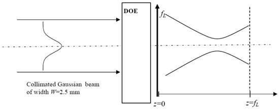
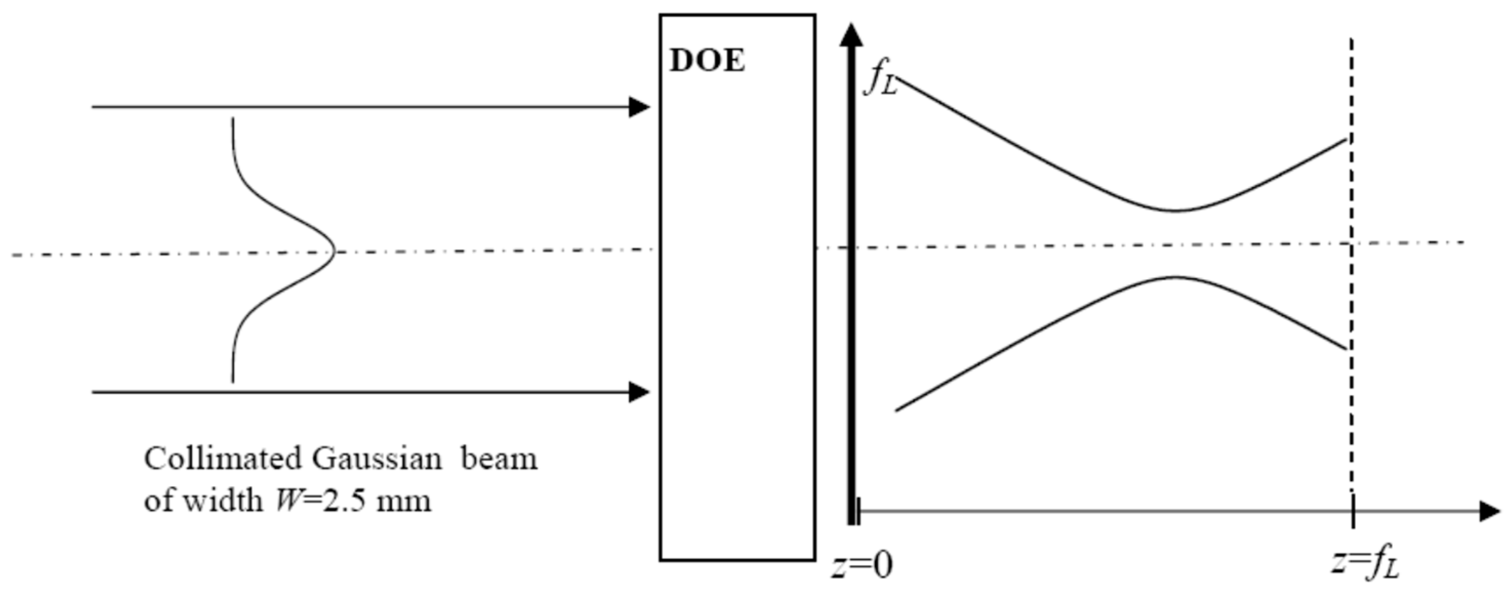
The geometry of GB reshaping is given in Figure 1, which shows a collimated GB having a width W incident on the couple (DOE + focusing lens).

Figure 1. Setup showing the geometry of the Gaussian beam reshaping by a DOE set as close as possible to the focusing lens of focal length f_L = 125 mm.

The incident collimated Gaussian beam is characterised by its electrical field $E_{in}$ given by

$$E_{in}(\rho )=E_0\times \exp [-{\rho }^2/W^2]$$

(3)

The incident GB diffracting on the DOE of transmittance $\tau (\rho )$, and focused by the lens of focal length f_L = 125 mm, gives rise to the diffracted electric field $E_d(r,z)$ handled by the well-known Fresnel–Kirchhoff integral given by

$$E_d(r,z)={\displaystyle \frac{2\pi }{\lambda z}}{\displaystyle \underset{0}{\overset{\infty }{\int }}\tau (\rho )E_{in}(\rho )}\exp \left[{\displaystyle \frac{i\pi {\rho }^2}{\lambda }}\left({\displaystyle \frac{1}{f_L}}-{\displaystyle \frac{1}{z}}\right)\right]J_0\left[{\displaystyle \frac{2\pi }{\lambda z}}r.\rho \right]\rho d\rho$$

(4)

where r is the radial coordinate in plane z, and $J_0$ is the zero-order Bessel function of first order. Equation (4) allows the determination of the transverse distribution of the diffracted field $E_d(r,z)$ in any plane z, and the on-axis diffracted field $E_d(r=0,z)$. The intensity distribution $I_d(r,z)$ is proportional to the square of the electric field: $I_d(r,z)\prec {\left|E_d(r,z)\right|}^2$. The Fresnel–Kirchhoff integral is calculated numerically by using a FORTRAN routine involving the numerical integrator dqdag from the International Mathematics and Statistical Library (IMSL). The transmittance $\tau (\rho )$ appearing in Equation (4) stands for ${\tau }_1(\rho )$ $({\tau }_2(\rho ))$ for DOE#1 (DOE#2).

2.1. Monochromatic Beam Reshaping Using DOE#1

At first glance, it appears that fabricating DOE#1 with a transmittance $\cos (\beta {\rho }^2)$ cannot be achieved through the simple etching of a transparent glass piece. Indeed, DOE#1 acts on both phase and amplitude. However, it has been demonstrated in [56] that generating a transmittance $\cos (\beta {\rho }^2)$ is possible using a phase-only spatial light modulator (SLM). This procedure is advantageous because the parameter $\beta$ can be continuously adjusted, allowing flexible control of the reshaped beam profile.

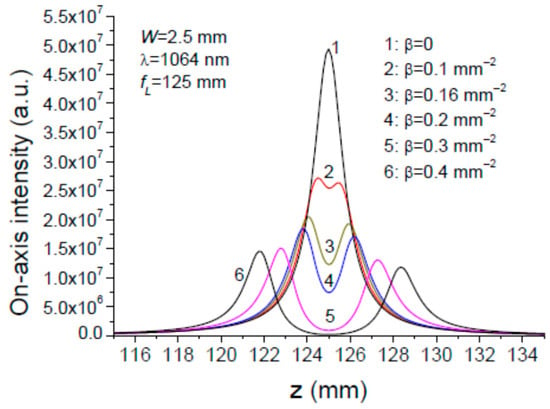
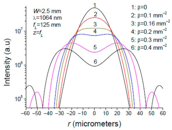
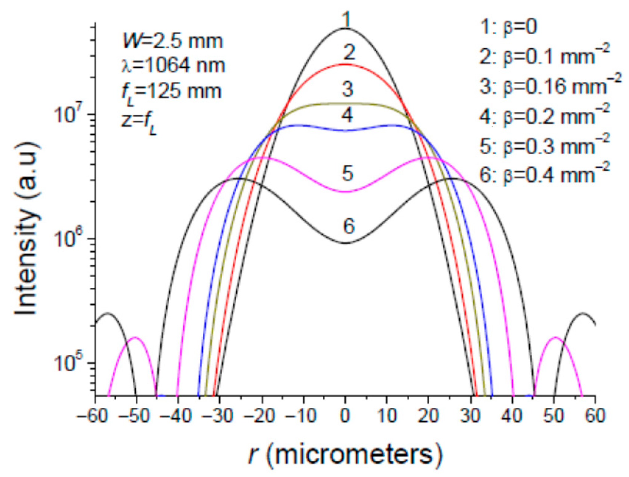
The diffraction of the collimated Gaussian beam of width W = 2.5 mm upon the couple (DOE#1 + converging lens) according to Figure 1 is characterised by two intensity distributions. The first one, shown in Figure 2, is the on-axis intensity $I_d(r=0,z)$ as a function of the longitudinal coordinate z. The second one is the radial intensity distribution $I_d(r,z=f_L)$ plotted in Figure 3. The plots in Figure 2 and Figure 3 represent several values of parameter $\beta$.

Figure 2. On-axis intensity distribution (r = 0) of a collimated Gaussian beam of width W = 2.5 mm diffracting on DOE#1 having a transmittance ${\tau }_1(\rho )=\cos (\beta {\rho }^2)$, followed by a converging lens of focal length f_L = 125 mm.

Figure 3. Radial intensity distribution in the focal plane z = f_L of a Gaussian beam diffracting on the couple (DOE#1 + converging lens) for different values of parameter $\beta$.

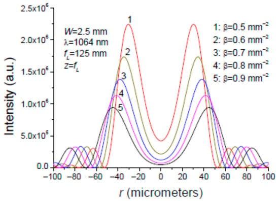
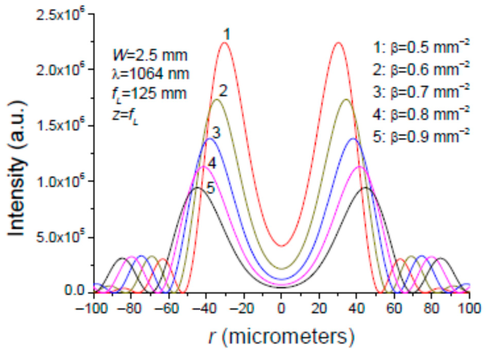
It is seen in Figure 2 and Figure 3 that the flat-top (FT) intensity distribution in plane $z=f_L$ is obtained for $\beta =0.16{ \mathrm{mm}}^{-2}$, while the OBB is obtained for several values of parameter $\beta$ as shown in Figure 4. As the control parameter $\beta$ increases, it is observed that the ring’s intensity decreases while its diameter increases, and the central intensity at r = 0 diminishes.

Figure 4. Radial intensity distribution in the focal plane z = f_L of a Gaussian beam diffracting on the couple (DOE#1 + converging lens) for different values of parameter $\beta$.

In a first step, as indicated above, the DOE#1 with the transmittance $\cos (\beta {\rho }^2)$ was achieved by using an SLM. The capacity of this diffractive optical element to transform a Gaussian beam into a doughnut or a flat-top profile has been experimentally proven in the monochromatic case [56]. It is worth emphasising that SLMs are versatile and programmable, but are made up with liquid crystal, which has the property of being sensitive to wavelength [52,56,57,58,59], and consequently are not well adapted to the beam reshaping of broadband light beams.

In a second step, the term $\cos (\beta {\rho }^2)$ that modulates the incident GB was achieved using a Michelson interferometer, which superposes two coherent GBs coaxially from its arms. Experimental results have shown that this monochromatic GB superposition yields a flat-top or an OBB in the focal plane of a focusing lens. This interferometric beam shaping technique is described in the Appendix A for the monochromatic case, and how it can be adapted to a spectrally broadened Gaussian beam is considered in detail.

2.2. Monochromatic Beam Reshaping Using the DOE#2

DOE#2, having a complex transmittance given by Equation (2), is a binary diffractive optical element (called as π-plate) which introduces a π-phase shift in the central part of the incident collimated Gaussian beam. The π-plate under consideration is made up of a transparent material of refractive index $n_0$ in which a relief of depth $\delta =\lambda /\left[2(n_0-1)\right]$ is etched. The relief shape is a circle of radius ${\rho }_0$. The intensity profile $I_d(r,z=f_L)$ is controlled by the parameter $Y_{PI}$ defined by

$$Y_{PI}={\rho }_0/W$$

(5)

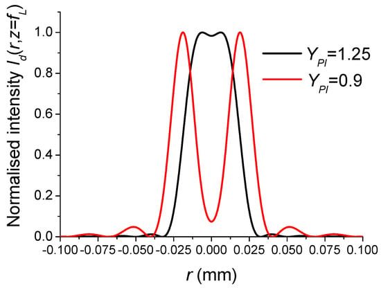
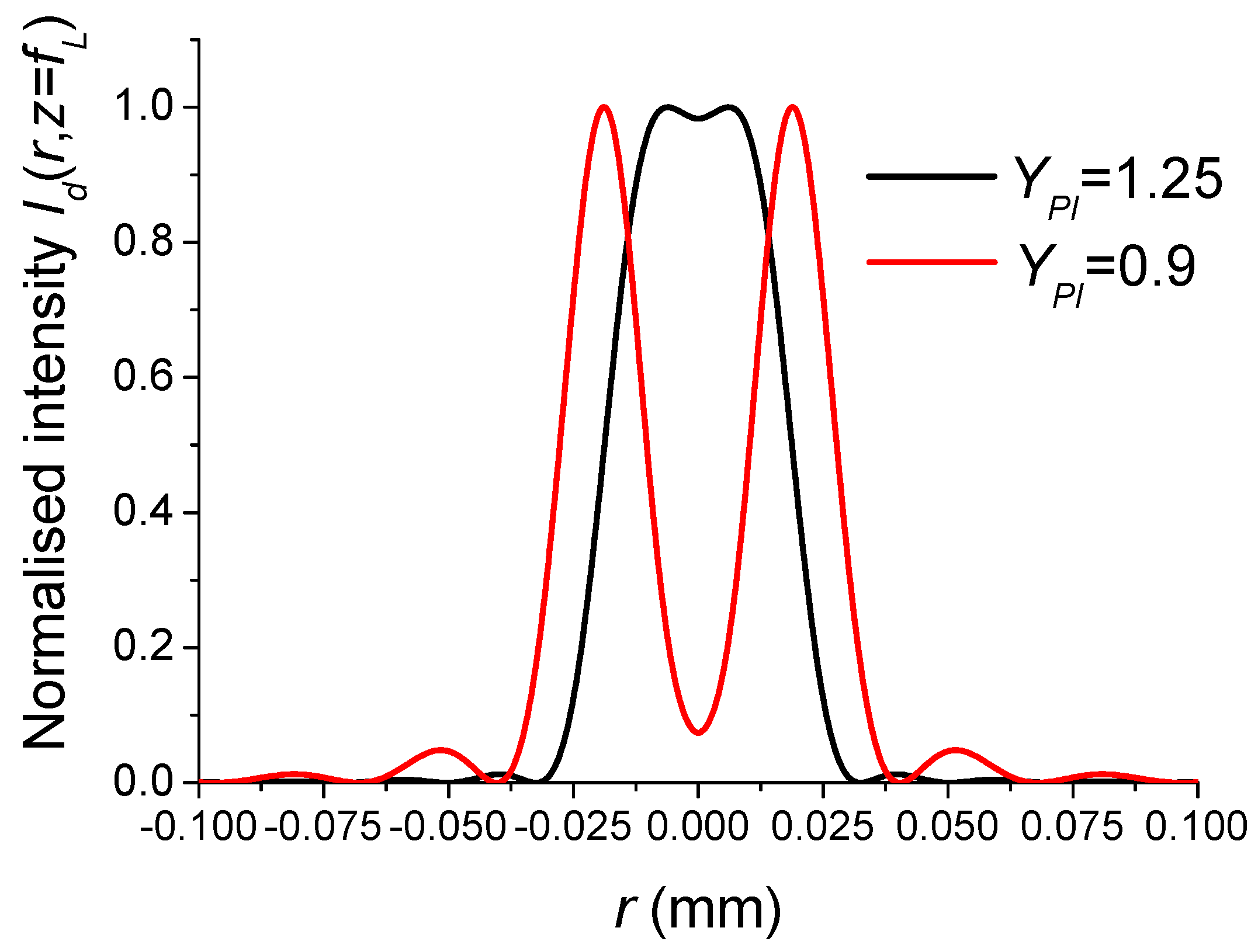
The two intensity profiles of interest, flat-top and OBB shown in Figure 5, are obtained for $Y_{PI}=1.25$ and 0.9, respectively [60].

Figure 5. Intensity profile in the plane $z=f_L$ showing the capacity of the π-plate to transform a Gaussian beam of width W = 2.5 mm into a flat-top or a doughnut profile. The focusing lens has a focal length f_L = 125 mm. The incident beam is monochromatic with a wavelength λ = 1064 nm.

3. Reshaping of a Gaussian Broadband Beam Using an Interferometer and DOE#2

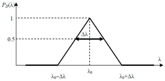
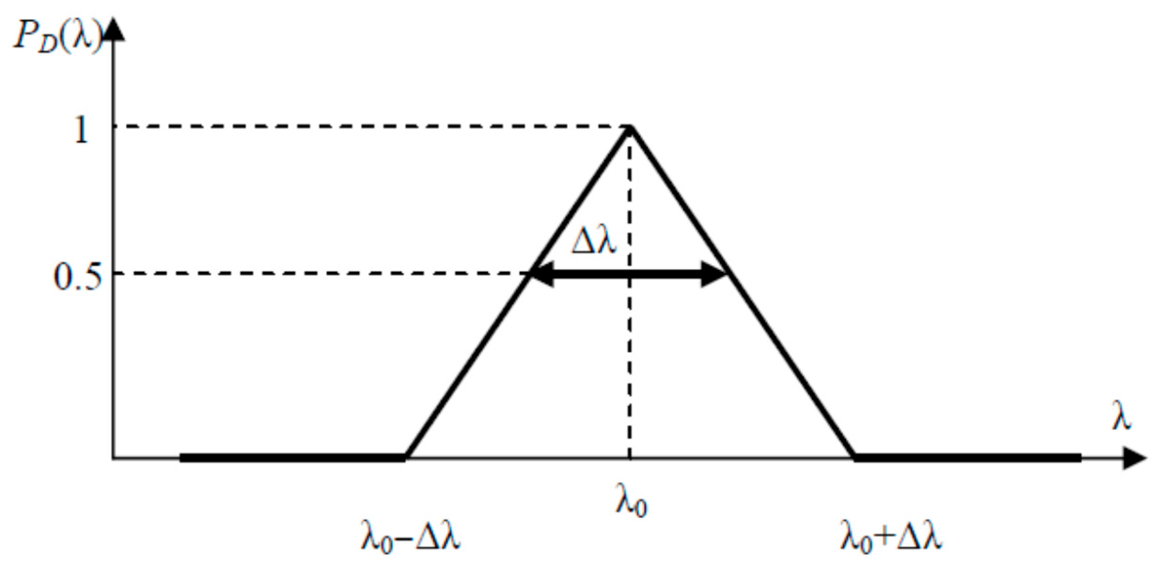
The Gaussian beam that is to be reshaped is no longer monochromatic, but is characterised by its normalised spectral power distribution $P_D(\lambda )$, which has a full width at half maximum (FWHM) $\mathsf{\Delta }\lambda$. The spectral light distribution is typically bell-shaped, and can be Gaussian or Lorentzian, centred on a particular wavelength ${\lambda }_0$ and having a width of FWHM $\mathsf{\Delta }\lambda$. For simplicity, we will consider the triangular spectral distribution shown in Figure 6.

Figure 6. Spectral distribution of the incident polychromatic Gaussian beam.

The distribution $P_D(\lambda )$ shown in Figure 6 is modelled by the following equation:

$$P_D(\lambda )=\left\{\begin{array}{l}0 \hspace{1em}\hspace{1em}\hspace{1em}\hspace{1em}\mathrm{for} \lambda <({\lambda }_0-\mathsf{\Delta }\lambda )\\ 1+{\displaystyle \frac{\lambda -{\lambda }_0}{\mathsf{\Delta }\lambda }}\hspace{1em}\mathrm{for} ({\lambda }_0-\mathsf{\Delta }\lambda )\le \lambda \le {\lambda }_0 \\ 1+{\displaystyle \frac{{\lambda }_0-\lambda }{\mathsf{\Delta }\lambda }}\hspace{1em}\mathrm{for} {\lambda }_0\le \lambda \le ({\lambda }_0+\mathsf{\Delta }\lambda ) \\ 0 \hspace{1em}\hspace{1em}\hspace{1em}\hspace{1em}\mathrm{for} \lambda >({\lambda }_0+\mathsf{\Delta }\lambda ) \end{array}\right.$$

(6)

The power carried by the polychromatic incident GB is proportional to its squared electric field so that the electric field given in Equation (3) is rewritten as follows:

$$E_{in}(\rho ,\lambda )=E_0\times \sqrt{P_D(\lambda )}\times \exp [-{\rho }^2/W^2]$$

(7)

3.1. Polychromatic Beam Reshaping Using a Michelson Interferometer

In view of the above, we must consider an alternative to using the usual SLMs to generate the modulation term ${\tau }_1(\rho )=\cos (\beta {\rho }^2)$ suitable for a broadband beam. One possible solution is the interferometric beam shaping technique, which uses a Michelson interferometer to achieve the coaxial superposition of two Gaussian beams with the same width (W) and opposite radii of curvature: (W,+R) and (W,−R). This interferometric method is explained in greater detail in the Appendix A, so we will not reiterate its presentation here. However, it is important to remember that the beam reshaping ability of the Michelson interferometer (MI) is highly dispersive when its arms have different lengths, i.e., $D_1\ne D_2$. Consequently, the Appendix A shows that MI dispersion is significantly reduced when the MI is symmetric, i.e., $D_1=D_2$. In this case, producing the two Gaussian beams, (W,+R) and (W,−R), in the plane of the focusing lens is possible by replacing the MI’s usual plane mirrors with a convex mirror and a concave mirror, as shown in Figure A7. However, there is still an inevitable dispersion due to the wavelength dependence of the parameter $\beta$ given in Equation (A3). For convenience, the dimensionless parameter K is introduced in place of the parameter $\beta$, so that the modulation term ${\tau }_1(\rho )$ takes the following form:

$${\tau }_1(\rho )=\cos (\beta {\rho }^2)=\cos \left({\displaystyle \frac{2\pi K}{W_e^2}}{\rho }^2\right) \mathrm{with} K={\displaystyle \frac{W_e^2}{2\lambda R_M}}$$

(8)

where $R_M$ and $W_e$ refer to the mirror radius of curvature and incident collimated Gaussian beam width, respectively (see Figure A7). As shown in the Appendix A, the value of interest for parameter K which controls beam shaping is K = 0.16 (0.4) for a flat-top (doughnut) intensity profile.

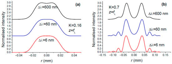
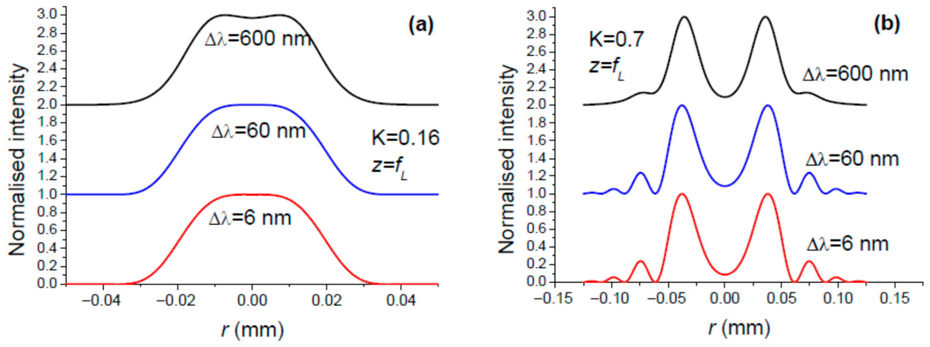
Taking Equation (8) into account, we can expect the spatial reshaping of the incident polychromatic GB to differ according to the spectral region. Consequently, the intensity profile in the focal plane of the focusing lens (Figure A7) is the result of the superposition of intensity profiles associated with the different spectral regions, which leads to a blurring of the reshaping. However, the plots in Figure 7 contradict this intuitive weakness, demonstrating the robustness of interferometric beam reshaping with respect to the spectral bandwidth of the incident Gaussian beam.

Figure 7. Intensity distribution in the focal plane of the focusing lens L for the three values of bandwidth $\mathsf{\Delta }\lambda$, and two remarkable values for parameter K: (a) K = 0.16 for the conversion of GB to FT, and (b) K = 0.7 for the conversion of GB to OBB. The central wavelength is λ₀ = 1064 nm.

In light of the above, we should not presume that the interferometric reshaping technique is infallible when the input beam is spectrally broadened. To illustrate this, consider the case of femtosecond laser pulses, which are characterised by a spectral frequency bandwidth $\mathsf{\Delta }\nu$ (FWHM). According to the following relation [42], the latter is inversely proportional to the pulse duration $t_p$ (FWHM) for a sech² pulse:

$$t_p\times \mathsf{\Delta }\nu =0.315$$

In addition, it is important to consider the spatial extent $\mathsf{\Delta }z$ of the pulse:

$$\mathsf{\Delta }z=c\times t_p$$

where c is the light speed. Table 1 shows the order of magnitude of the quantities $t_p$, $\mathsf{\Delta }\lambda$ and $\mathsf{\Delta }z$.

Table 1. Relationship between the duration $t_p$, the spectral bandwidth $\mathsf{\Delta }\lambda$, and the spatial length $\mathsf{\Delta }z$ of femtosecond pulses.

${\mathit{t}}_{\mathit{p}}$ in fs	1	10	100
$\mathsf{\Delta }\lambda$ in nm	1000	100	10
$\mathsf{\Delta }z$ in µm	0.3	3	30

In the setup shown in Figure A7, the focusing lens L is illuminated by two Gaussian beams, ($W_e,R_M$) and ($W_e,-R_M$), which focus at different positions, respectively, at distances $z_{\max 1}$ and $z_{\max 2}$. This is illustrated in Figure 2, where the on-axis intensity has two maxima occurring from both sides of the geometrical focus position $z=f_L$ as parameter $\beta$ is increased. The positions $z_{\max 1}$ and $z_{\max 2}$ are given by the following relations [61]:

$$z_{\max 1}={\displaystyle \frac{\left(\frac{1}{f_L}-\frac{1}{R_M}\right)}{{\left(\frac{1}{R_M}-\frac{1}{f_L}\right)}^2+{\left(\frac{2}{k{W}_e^2}\right)}^2}}$$

(9)

$$z_{\max 2}={\displaystyle \frac{\left(\frac{1}{R_M}+\frac{1}{f_L}\right)}{{\left(\frac{1}{R_M}+\frac{1}{f_L}\right)}^2+{\left(\frac{2}{k{W}_e^2}\right)}^2}}$$

(10)

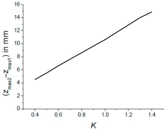
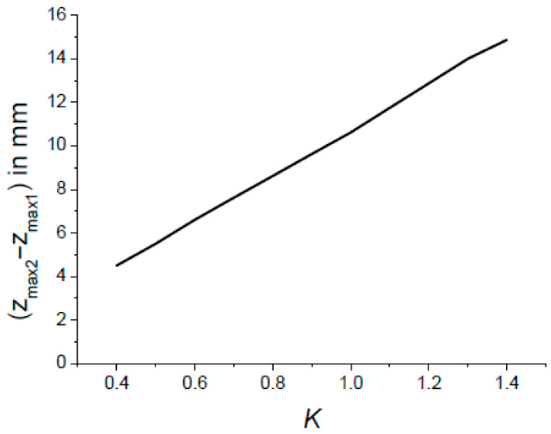
Now, we have to compare the distance ($z_{\max 2}$ − $z_{\max 1}$) to the spatial extent $\mathsf{\Delta }z$ of the pulse in order to determine if the necessary overlapping of the two pulses associated with the two GBs, ($W_e,R_M$) and ($W_e,-R_M$), is possible or not. This overlapping occurs as the inequality $(z_{\max 2}-z_{\max 1})<\mathsf{\Delta }z$ is satisfied. Figure 8 shows the variations in ($z_{\max 2}$ − $z_{\max 1}$) versus the parameter K. The latter varies according to the mirror radius of curvature $R_M$, as defined in Equation (8), and evaluated at the central wavelength $\lambda ={\lambda }_0=1064$ nm. Upon closer inspection of Figure 8, it can be concluded that interferometric beam shaping is not applicable to ultrashort pulses, as the distance ($z_{\max 2}$ − $z_{\max 1}$) between the best focal points associated with the GB ($W_e,R_M$) and ($W_e,-R_M$) is far greater than the pulse length $\mathsf{\Delta }z$ given in Table 1. Therefore, it can be concluded that interferometric beam reshaping using the setup shown in Figure A7 is not applicable to ultrashort pulses with a duration of less than 1 ps. However, interferometric beam reshaping could be successful for a spectrally broadened CW (continuous wave) beam or a pulsed laser beam with a spatial extent of a few tens of millimetres (i.e., a pulse duration greater than 150 ps if Δz > 50 mm).

Figure 8. Variations in the distance ($z_{\max 2}$ − $z_{\max 1}$) separating the best focus associated with the two Gaussian beams ($W_e,R_M$) and ($W_e,-R_M$) incident on the focusing lens L (see Figure A7). The parameters are W_e = 2.5 mm, f_L = 125 mm and λ₀ = 1064 nm.

3.2. DOE#2 for Reshaping a Polychromatic Gaussian Beam

DOE#2 was presented in Section 1. One assumes a collimated GB having a width W_e = 2.5 mm, spectrally broadened according to Figure 6, incident on the π-plate characterised by its transmittance ${\tau }_2(\rho )$ given by Equation (2). The π-plate is followed by a converging lens of focal length f_L = 125 mm. We are interested in the intensity profile $I_d(r,z=f_L)={\left|E_d(r,z=f_L)\right|}^2$ in the focal plane z = f_L where the diffracted field $E_d$ is

$$E_d(r,z=f_L)={\displaystyle \frac{2\pi }{\lambda f_L}}{\displaystyle \underset{-\infty }{\overset{+\infty }{\int }}{\displaystyle \underset{0}{\overset{+\infty }{\int }}{\tau }_2(\rho )E_{in}(\rho )}}\sqrt{P_D(\lambda )}{J}_0\left[{\displaystyle \frac{2\pi }{\lambda f_L}}r.\rho \right]\rho d\rho d\lambda$$

(11)

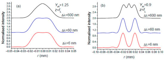
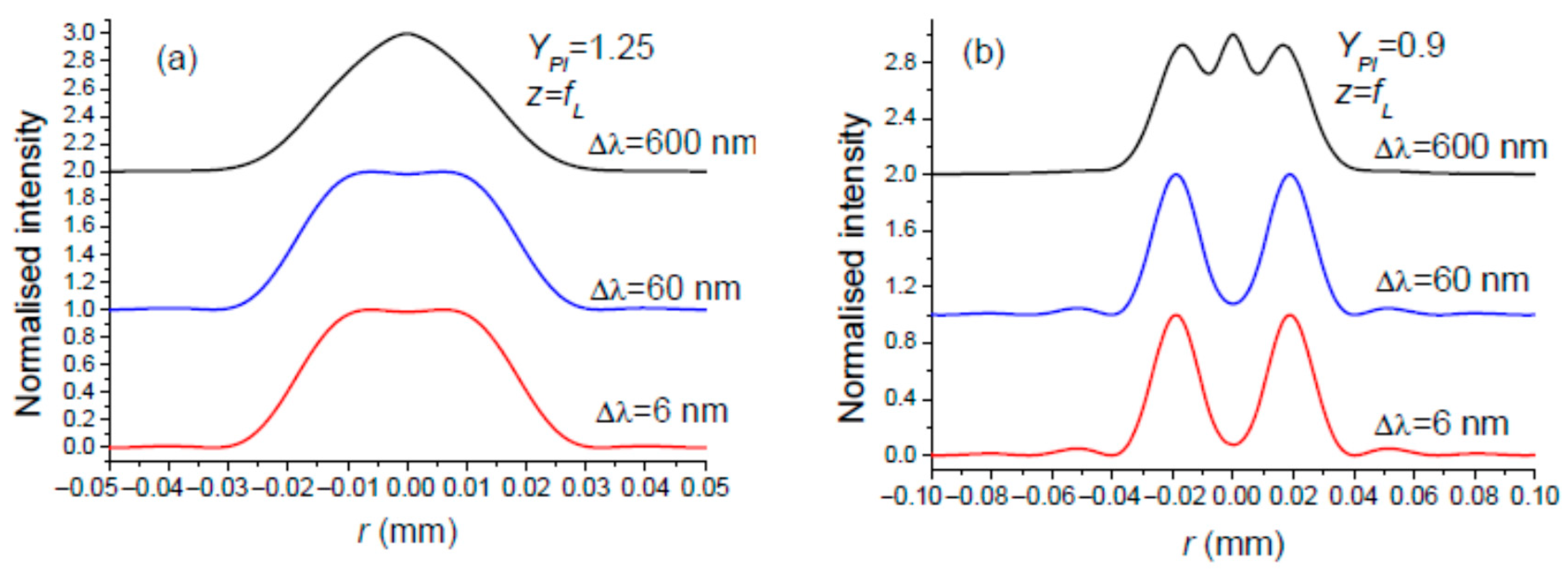
As for DOE#2 in the monochromatic case considered in Section 2.2, we will focus on the two notable Y_PI values leading to a flat-top or OBB, respectively: Y_PI = 1.25 and Y_PI = 0.9. Figure 9a,b show the results for three values of $\mathsf{\Delta }\lambda$. A quick glance at Figure 9 reveals that the beam reshaping carried out by the π-plate (DOE#2) becomes blurred, especially when the spectral bandwidth $\mathsf{\Delta }\lambda$ is large.

Figure 9. Intensity $I_d(r,z=f_L)\prec {\left|E_d(r,z=f_L)\right|}^2$ in the plane z = f_L when the incident Gaussian beam on a π-plate is spectrally broadened according to Figure 6. The central wavelength is λ₀ = 1064 nm, the collimated incident GB has a width of W_e = 2.5 mm, and the focal length of the focusing lens L is f_L = 125 mm. Nominal beam reshaping into (a) a flat-top and (b) a doughnut (OBB). The central wavelength is λ₀ = 1064 nm.

In any case, it is reasonable to state that interferometric beam shaping, used to transform a spectrally broadened Gaussian beam into a flat-top or an optical bottle beam, is more resistant to an increase in the spectral bandwidth of the incident beam than diffractive beam shaping using a π-plate.

4. Discussion

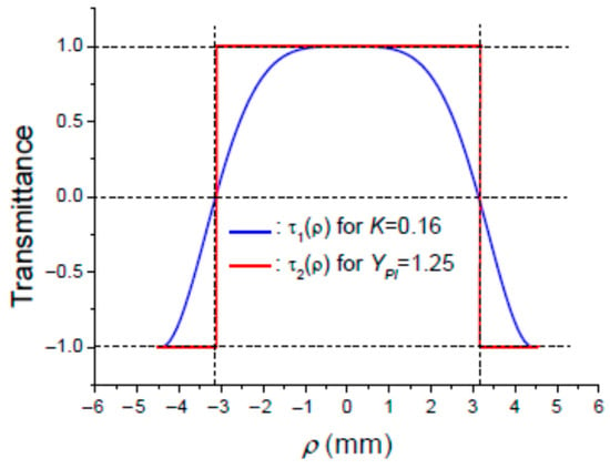
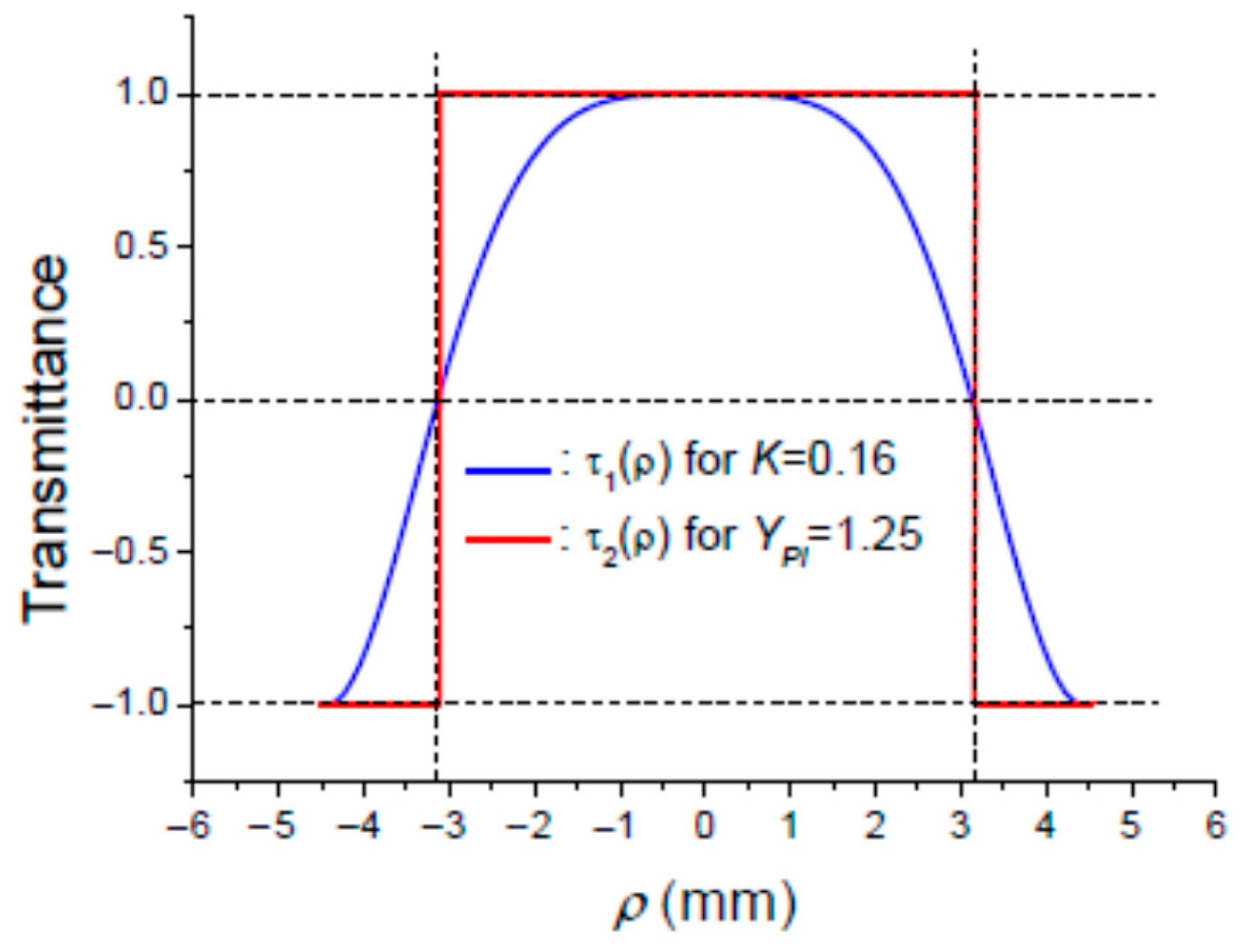
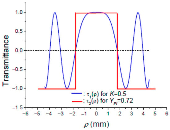
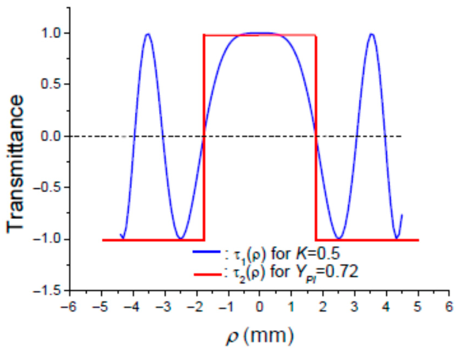
In view of the above, it can be concluded at least for the monochromatic enlightenment that both DOE#1 and DOE#2 are able to transform a Gaussian beam into a flat-top or an optical bottle beam. It would be interesting to know why the two transmittance profiles, ${\tau }_1(\rho )$ and ${\tau }_2(\rho )$, originating from interference and diffraction, respectively, have the same ability in terms of beam reshaping. One likely hypothesis that comes to mind is that the transmittance profiles ${\tau }_1(\rho )$ and ${\tau }_2(\rho )$ should be similar. To test this hypothesis, consider the plots of ${\tau }_1(\rho )$ and ${\tau }_2(\rho )$ in Figure 10, for $Y_{PI}=1.25$ and K = 0.16, and in Figure 11, for $Y_{PI}=0.9$ and K = 0.7, corresponding to an intensity profile in plane $z=f_L$ which is a flat-top or a doughnut, respectively. The value of $Y_{PI}$ used in Figure 10 and Figure 11 corresponds to the point of sign reversal of transmittance ${\tau }_1(\rho )$. The conclusion that can be drawn is that the modulating term ${\tau }_1(\rho )$ originating from the Michelson interferometer setup shown in Figure A7 behaves approximately as a π-plate having a smoother profile than the usual sharp one described in Equation (2). Note that the sign of ${\tau }_2(\rho )$ in Figure 10 and Figure 11 is the opposite of that in Equation (2). This difference is not significant since the beam reshaping achieved is the same whatever the DOE transmittance is, ${\tau }_2$ or $-{\tau }_2$.

Figure 10. Variations in transmittances: ${\tau }_1(\rho )$ for K = 0.16 and ${\tau }_2(\rho )$ for $Y_{PI}=1.25$.

Figure 11. Variations in transmittances: ${\tau }_1(\rho )$ for K = 0.5 and ${\tau }_2(\rho )$ for $Y_{PI}=0.72$.

Now, it would be useful to list the advantages and disadvantages in using DOE#1 and DOE#2 for transforming a Gaussian beam into a flat-top or a doughnut profile.

DOE#1 advantages:

-

High resiliency towards the spectral bandwidth of the incident beam to be reshaped. The transformation of a Gaussian beam into a flat-top or OBB profile remains unperturbed even for a large bandwidth $\mathsf{\Delta }\lambda$.

-

The interferometric beam shaping technique does not introduce any aberration in the reshaped beam.

-

The setup shown in Figure A7 allows for generating the modulating term ${\tau }_1(\rho )=\cos (\beta {\rho }^2)$ with high agility in the sense that the intensity profile in the focal plane of lens L could be rapidly changed from a flat-top to doughnut profile just by changing the radius of curvature of mirrors M₁ and M₂. This can be achieved by using a programmable liquid lens used as an add-on to a fixed focus lens [62,63,64,65].

-

The interferometric beam shaping technique using the setup shown in Figure A7 does not introduce any aberration in the reshaped beam.

DOE#1 disadvantages:

-

As with most interferometric devices, the setup shown in Figure A7 may be sensitive to temperature. Fluctuations in the ambient temperature cause a phase change in the light inside the arms of the Michelson interferometer. This could alter the intensity profile of the reshaped beam, as illustrated in Figure A4. In fact, this situation is probably not as disastrous as has been suggested, since the optical phase in each arm of the MI changes by the same amount with temperature changes, meaning that the setup shown in Figure A7 could be nearly temperature-insensitive. Nevertheless, it would be sensible to enclose the Michelson interferometer in a temperature-stabilised box.

-

The Michelson interferometer’s transmission rate is around 50%, leading to significant losses in the reshaped beam.

-

The interferometric beam shaping technique based on the setup shown in Figure A7 is well suited to continuous-wave (CW) beams. It does not work for ultra-short pulses with a duration of less than 1 ps, but it could work well for pulses with a duration greater than about 150 ps.

DOE#2 advantages:

-

The use of DOE#2 enables the beam reshaping setup to be more compact, since it only comprises a π-plate and a focusing lens.

-

Beam reshaping using DOE#2 works well for CW beams [15] and ultrashort pulses [66,67].

DOE#2 disadvantages:

-

The π-plate is a diffractive optical element which is relatively costly.

-

The use of a π-plate for reshaping a Gaussian beam is not a flexible technique, since changing the parameter $Y_{PI}$ requires changing the width W_e of the incident collimated Gaussian beam, which is not immediately possible.

-

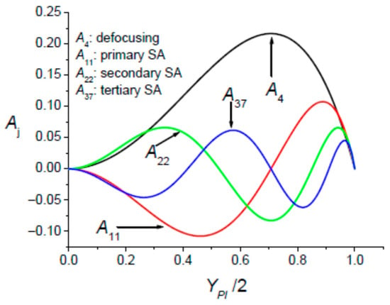
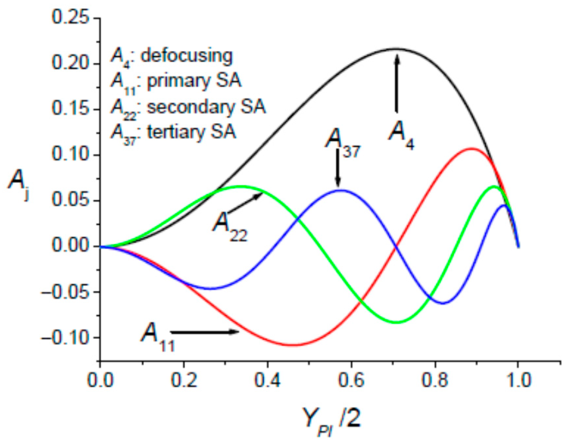
The collimated Gaussian beam passing through the DOE#2 has its wavefront distorted since it exhibits a discontinuity. As a result, the π-plate introduces optical aberrations in the reshaped beam. These diffractive aberrations have been characterised [68] by determining the aberration coefficients a_j in the framework of the modelling introduced by Mahajan [69]. The variations in the normalised defocusing and the high-order spherical aberration coefficients $A_j=a_j/\lambda$ are shown in Figure 12.

Figure 12. Variations in the normalised aberration coefficients A_j versus the parameter Y_PI. The π-plate produces defocusing and high-order spherical aberrations (SAs).

The issue of reshaping broadband Gaussian beams dates back a few years [50], but has recently been revived thanks to new devices such as digital micro-mirror devices [51].

5. Spatial Beam Reshaping of a Laser with Widely Tunable Wavelength

Without making any sweeping generalisations, it can be observed that any beam shaping technique based on reshaping the phase profile of the beam wavefront could be expected to be wavelength-dependent. This is the case for the DOE#1 and DOE#2 devices considered in the preceding sections. This wavelength dependence could pose a significant challenge if we wish to reshape the Gaussian beam delivered by a widely tunable laser operating over a broad tuning range of several hundred nanometers [53,54,55]. Such lasers can be considered as monochromatic sources with tunable wavelengths over a more or less wide range. Consequently, if no action is taken, the desired intensity profile in the focal plane of a focusing lens could be lost when the laser wavelength is tuned. To keep the reshaped intensity profile unchanged when the wavelength is tuned, we must take action to mitigate the dispersion properties of the reshaping device. This problem has been addressed by A. Forbes et al. in [70] for a phase-only DOE. Without going into the reasoning behind the method used by the authors of [70] to compensate for the dispersion of the DOE, which is assumed to achieve a Gaussian-to-Flat-Top-beam transformation, we present the solution proposed by A. Forbes et al.: by displacing the observation plane, the desired intensity mapping, which is lost in the focal plane of the focusing lens when the wavelength is tuned, can be recovered. Note that this method of beam shaping dispersion compensation is not very practical, since a tracking system is required to observe the particular plane where the desired intensity mapping occurs as the operating wavelength is tuned. This drawback can be avoided by using the interferometric beam shaping method with the setup shown in Figure A7. The cause of beam shaping dispersion is that the key parameter K, which controls intensity mapping in the plane $z=f_L$, is inversely proportional to the operating wavelength, as shown in Equation (8). To achieve beam reshaping in plane $z=f_L$ that is independent of the operating wavelength, the radius of curvature $R_M$ must be adjusted. As discussed in Section 4, this can be achieved by setting up a programmable liquid lens [62,63,64,65] in front of the Michelson interferometer mirrors.

6. Conclusions

This work presents a theoretical analysis of the reshaping of a spectrally broadened Gaussian beam into flat-top and optical bottle beam (OBB) intensity profiles using interferometric (Michelson interferometer) and diffractive (π-plate) approaches. While both techniques are effective in the monochromatic case and were experimentally verified ten years ago [15], pronounced differences arise under broadband illumination. The ability of the diffractive π-plate to shape beams is strongly sensitive to the spectral bandwidth, resulting in progressive degradation of the reshaped intensity profiles due to wavelength-dependent phase modulation. In contrast, the interferometric beam shaping technique is based on the coaxial superposition of two Gaussian beams, ($W_e,R_M$) and ($W_e,-R_M$). The target intensity profiles remain largely preserved over a wide spectral range. This robustness originates from the continuous nature of the interferometric modulation term $\cos (\beta {\rho }^2)$, and the absence of additional aberrations, since adding two spherical wavefronts does not introduce any aberration. While this approach is not suitable for ultrashort pulses, it is particularly well adapted to broadband continuous-wave (CW) sources and relatively long pulses (with a duration greater than about 150 ps). Overall, the present results establish interferometric beam shaping as an efficient and flexible solution for applications requiring broadband operation and precise control of the focal intensity distribution.

The issue of beam shaping stability with respect to wavelength also affects quasi-monochromatic beams delivered by a widely tunable laser. We have proposed a simple method applicable to interferometric beam shaping that mitigates the wavelength dependence of the reshaped beam’s intensity profile. This method involves locking the curvatures of the interferometer mirrors to the laser wavelength using programmable liquid lenses positioned in front of the mirrors.

Appendix A.1. The Gaussian Beam to Be Reshaped Is Monochromatic

An alternative to a diffractive optical element with a transmittance $\cos (\beta {\rho }^2)$ is the coaxial superposition of two Gaussian beams (GBs) with the same width W and opposite radii of curvature in a given plane: (W,R) and (W,−R). This particular longitudinal position where the two GBs, (W,R) and (W,−R), interfere is precisely where the focusing lens of focal length $f_L$ should be positioned. The intensity profiles of interest are either a flat-top or doughnut-shaped intensity distribution, which are expected in the focal plane of the focusing lens. The resulting electric field $E_L$, in the plane of the focusing lens, associated with the coaxial superposition of GBs (W,R) and (W,−R) takes the following form:

$$E_L(\rho )=E_0\exp \left[-i{\displaystyle \frac{k{\rho }^2}{2R}}\right]\exp ‖-{\displaystyle \frac{{\rho }^2}{W^2}}‖+E_0\exp \left[+i{\displaystyle \frac{k{\rho }^2}{2R}}\right]\exp ‖-{\displaystyle \frac{{\rho }^2}{W^2}}‖$$

(A1)

$$E_L(\rho )=2E_0\cos \left[{\displaystyle \frac{k{\rho }^2}{2R}}\right]\exp ‖-{\displaystyle \frac{{\rho }^2}{W^2}}‖$$

(A2)

Note that in Equation (A1), we kept only the useful terms, allowing for the term $\cos (\beta {\rho }^2)$ to be generated. Taking into account Equation (1) allows for the parameter $\beta$ to be identified:

$$\beta ={\displaystyle \frac{\pi }{\lambda R}}$$

(A3)

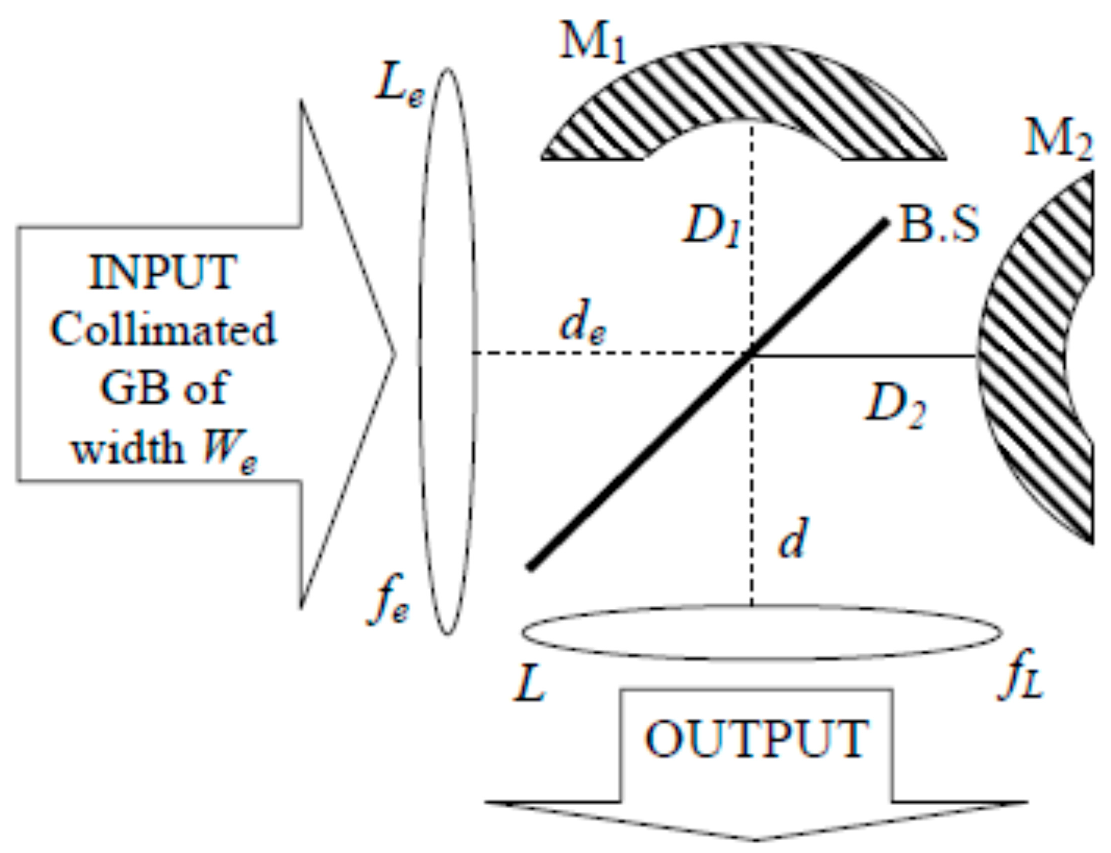
The coaxial superposition of the two coherent monochromatic Gaussian beams can be achieved by using a Michelson interferometer as shown in Figure A1. In the plane of the focusing lens L there is a superposition of two beams: beam#1 and beam#2. Beam#1 in the plane of L is a GB (W,−R), which has travelled a distance of $\left\{d_e+2D_2+d\right\}$ from the input lens L_e. Beam#2 in the plane of lens L is a GB (W,+R), which has travelled a distance of $\left\{d_e+2D_2+d\right\}$ from the input lens L_e. This arrangement is well described in Figure A2. It allows an adequate choice of parameters $\left\{d_e,D_2,D_1,f_e,d\right\}$.

Figure A1. Scheme of the Michelson interferometer (MI) allowing the transformation of a Gaussian beam into a flat-top or doughnut profile in the focal plane of lens L. The MI is made up of two plane mirrors and a beam-splitter, 50–50%.

Figure A1. Scheme of the Michelson interferometer (MI) allowing the transformation of a Gaussian beam into a flat-top or doughnut profile in the focal plane of lens L. The MI is made up of two plane mirrors and a beam-splitter, 50–50%.

Figure A2. Representation of the focused Gaussian beam by the input lens L_e inside the two arms of the Michelson interferometer used for generating the coaxial superposition of two coherent Gaussian beams.

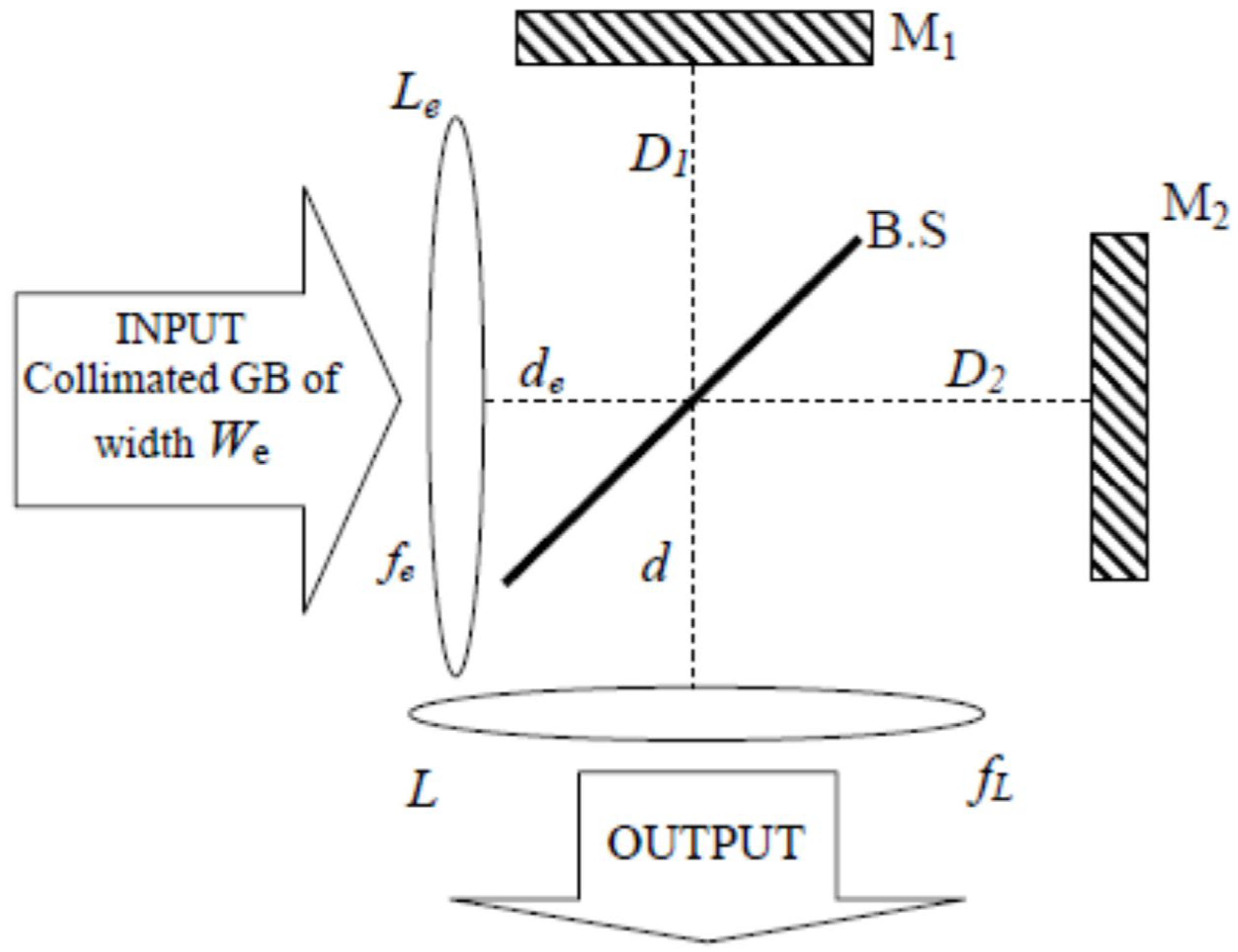
Figure A2. Representation of the focused Gaussian beam by the input lens L_e inside the two arms of the Michelson interferometer used for generating the coaxial superposition of two coherent Gaussian beams.

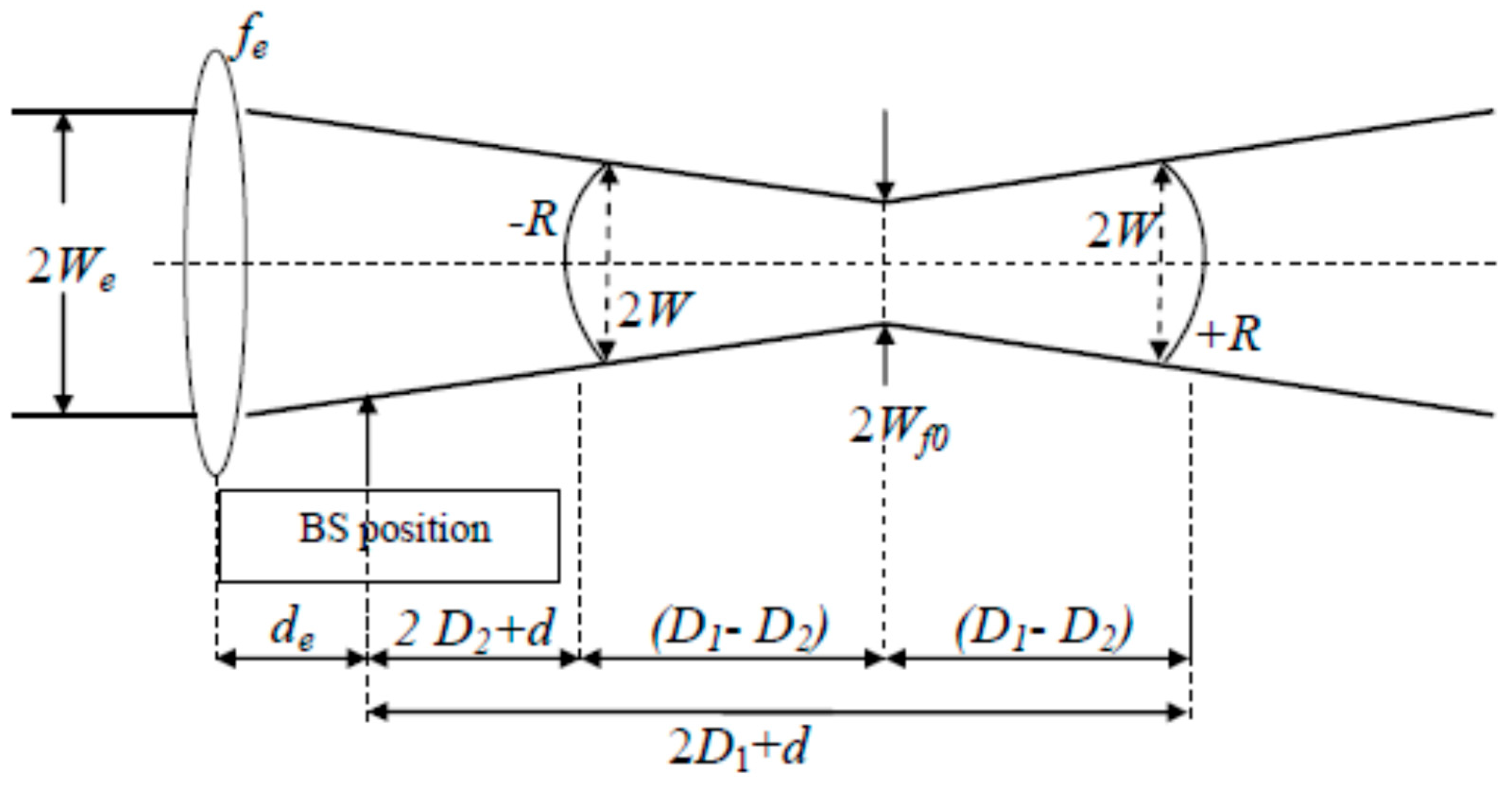
The location of the beam-waist plane of the GB focused by lens L_e is not random. The focal length f_e must satisfy the following equation:

$$f_e\approx d_e+d+D_1+D_2$$

(A4)

In a first step, the distances $\left\{d_e,d,D_2\right\}$ are chosen arbitrarily, and in a second step, adequate positioning of the beam-waist point has to be determined following two conditions: (i) the focal point of beam#2 reflected by mirror M₂ has to be located after lens L, and (ii) the focal point of the beam#1 reflected by mirror M₁ has to be located before lens L. The focused Gaussian beam by lens L_e is characterised by its beam-waist size $W_{f0}$ given by

$$W_{f0}\approx {\displaystyle \frac{\lambda f_e}{\pi W_e}}$$

(A5)

If we set the origin z = 0 of the longitudinal axis in the plane of the input lens L_e, then the variations in W_f and R_f, the width and radius of curvature, respectively, of the focused (by lens L_e) input GB are given by

$$W_f(z)=W_{f0}\sqrt{1+{\left({\displaystyle \frac{z-f_e}{z_R}}\right)}^2}$$

(A6)

$$R_f(z)=(z-f_e)\left[1+{\left({\displaystyle \frac{z_R}{z-f_e}}\right)}^2\right]$$

(A7)

where $z_R=\pi W_{f0}^2/\lambda$ is the Rayleigh distance of the focused GB (by lens L_e). In the plane of the output lens L, the radius of curvature R is given by

$$R=\left[(D_1-D_2)+{\displaystyle \frac{z_R^2}{(D_1-D_2)}}\right]$$

(A8)

Consequently, as long as $W_e$ and $f_e$ are chosen, then the value of the control parameter $\beta$ depends only on the difference in arm lengths of the Michelson interferometer:

$$\beta ={\displaystyle \frac{\pi }{\lambda \left[(D_1-D_2)+\frac{z_R^2}{(D_1-D_2)}\right]}}$$

(A9)

The modulation term $\cos (\beta {\rho }^2)$ suffers greater or fewer variations depending upon the width W of the Gaussian term in the plane of the output lens L. Consequently, it is convenient to introduce a dimensionless parameter denoted K and defined as follows:

$$2\pi K=\beta W^2\to \beta ={\displaystyle \frac{2\pi K}{W^2}}\to K={\displaystyle \frac{W^2}{2\lambda R}}$$

(A10)

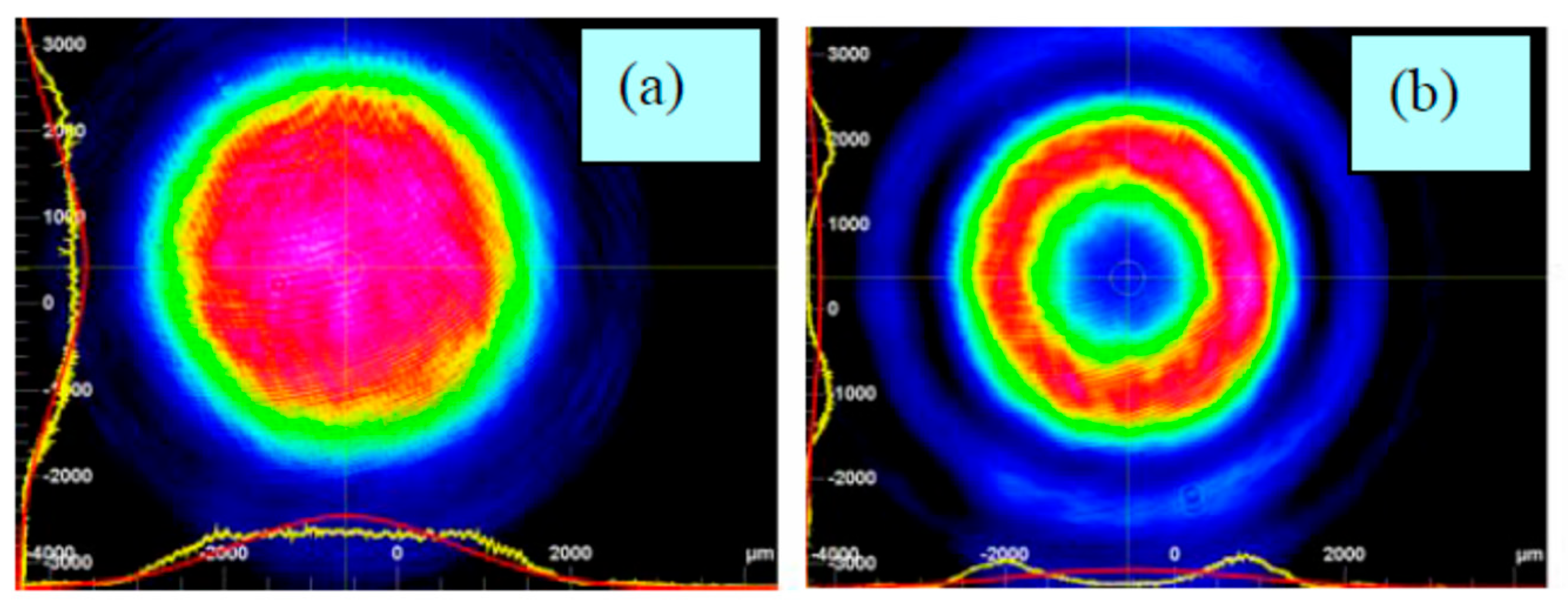
Two particular values for K have been identified for which the intensity profile in the focal plane of lens L is a flat-top for K = 0.16 or a doughnut for K = 0.4, as shown in Figure A3. Note that when the Gaussian beam is modulated by the DOE#1 of transmittance ${\tau }_1(\rho )=\cos (\beta {\rho }^2)$, it is found that the best doughnut, i.e., the deepest hollow, is obtained for K = 0.7 (or $\beta =0.9$ mm⁻²) as shown in Figure 4.

Let us return to the question of the interference, in the plane of lens L, of the field $E_1$ and $E_2$ originating from mirrors M₁ and M₂, respectively:

$$E_1=E_0{\displaystyle \frac{W_{f0}}{W(z)}}{e}^{-{\rho }^2/W^2}.\exp \left[-i\left\{k(D_1-D_2)-\varphi +{\displaystyle \frac{k{\rho }^2}{2R(z)}}\right\}\right]$$

(A11)

$$E_2=E_0{\displaystyle \frac{W_{f0}}{W(z)}}{e}^{-{\rho }^2/W^2}.\exp \left[+i\left\{k(D_1-D_2)-\varphi +{\displaystyle \frac{k{\rho }^2}{2R(z)}}\right\}\right]$$

(A12)

Figure A3. Experimental intensity patterns [15] in the focal plane of the output lens L: (a) for K = 0.16, i.e., (D₁ − D₂) = 2.4 mm; (b) for K = 0.4, i.e., (D₁ − D₂) = 5.4 mm.

Figure A3. Experimental intensity patterns [15] in the focal plane of the output lens L: (a) for K = 0.16, i.e., (D₁ − D₂) = 2.4 mm; (b) for K = 0.4, i.e., (D₁ − D₂) = 5.4 mm.

The distance travelled by the field $E_1$($E_2$) since the input lens L_e is ${\mathsf{\Delta }}_1=d_e+2D_1+d$ (${\mathsf{\Delta }}_2=d_e+2D_2+d$) in accordance with Figure A2. The phase shift $\varphi$ appearing above is the Gouy phase shift given by

$$\varphi =Arctg\left({\displaystyle \frac{D_1-D_2}{z_R}}\right)=Arctg\left\{{\displaystyle \frac{\lambda (D_1-D_2)}{\pi W_{f0}^2}}\right\}$$

(A13)

The quantity K, which is the control parameter of the beam reshaping in the focal plane of output lens L, takes the following form:

$$K={\displaystyle \frac{(D_1-D_2)}{2\pi z_R}}={\displaystyle \frac{(D_1-D_2)W_e^2}{2\lambda f_e^2}}$$

(A14)

A close look at Equation (A14) might suggest that the beam reshaping shown in Figure A3 occurs at any position of the output lens L. However, this is not the case, as there is only one position at which the two Gaussian beams originating from the Michelson interferometer take the forms (W, +R) and (W, −R).

The field $E_L=(E_1+E_2)$ at the input of lens L takes the following form:

$$E_L=2E_0{\displaystyle \frac{W_{f0}}{W(D_1-D_2)}}{e}^{-{\rho }^2/W^2(D_1-D_2)}\times \cos \left\{k(D_1-D_2)-\varphi +\beta {\rho }^2\right\}$$

(A15)

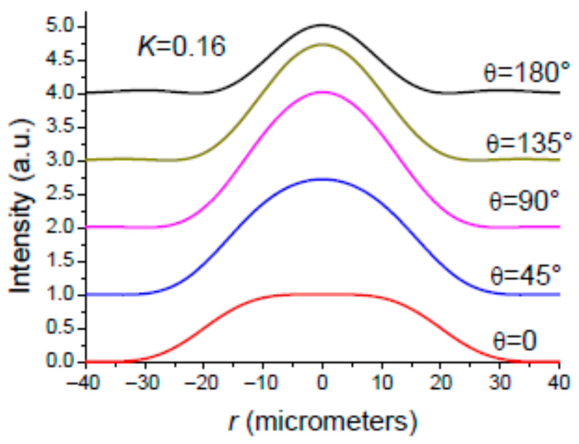
Let us introduce the angle $\theta =k(D_1-D_2)-\varphi$ appearing in Equation (A15). The angle $\theta$ varies with the wavelength and the interferometer arm length difference $(D_1-D_2)$. For reference to the Michelson interferometer behaviour for plane waves, the angle $\theta$ has to be equal to $N\pi$(N integer) at resonance, representing the maximum transmission of the interferometer. It is important to distinguish between the macroscopic and microscopic values of the path difference $\mathsf{\Delta }=(D_1-D_2)$. The macroscopic PD is mechanically adjusted to 2.4 mm (5.4 mm) for obtaining a flat-top (OBB) profile as shown in Figure A3. The microscopic PD is a fraction of the wavelength that should be adjusted by a PZT mount supporting one of the mirrors, M₁ or M₂. In addition, we have to consider thermal effects yielding to a shift in the net value of angle $\theta$, moving the interferometer away from resonance. Another cause of the shift in angle $\theta$ is its dependence on wavelength. This could play an important role when the incident GB is a broadband beam. In order to have a clear idea of the influence of the angle $\theta$ on the intensity profile of the reshaped beam in plane $z=f_L$, we plotted in Figure A4 the intensity profile $I_d(r,z=f_L)$ for a monochromatic incident GB and for several values of angle $\theta$. It is seen that the reshaped beam shape can be lost for a variation in the value of angle $\theta$ originating from a variation in $(D_2-D_1)$ or $\lambda$.

Figure A4. Simulated results: The setup shown in Figure A1 is adjusted for delivering in plane z = f_L a flat-top for $\theta =0$. It is seen that the reshaped beam shape is lost as the angle $\theta$ is changing. Parameters: f_L = 125 mm; W_e = 2.5 mm.

Figure A4. Simulated results: The setup shown in Figure A1 is adjusted for delivering in plane z = f_L a flat-top for $\theta =0$. It is seen that the reshaped beam shape is lost as the angle $\theta$ is changing. Parameters: f_L = 125 mm; W_e = 2.5 mm.

Appendix A.2. The Gaussian Beam to Be Reshaped Is Spectrally Broadened

According to the monochromatic study, it is clear, by examining Equation (A15) and Figure A4, that the MI shown in Figure A1 with $D_1\ne D_2$ is inherently dispersive. Consequently, if we want to reshape the intensity profile of a spectrally broadened focused beam using the setup shown in Figure A1, we need to minimise its dispersion properties as much as possible. According to Equation (A15), this could be achieved if the MI was symmetric, i.e., $D_1=D_2$. However, by doing this, we should obtain two identical Gaussian beams, (W, +R) and (W, +R), in the plane of the output lens L. Consequently, we must find a solution that allows us to obtain one Gaussian beam (GB) with a positive radius of curvature (ROC), and a second Gaussian beam with a negative ROC in the plane of L. This can be achieved by replacing the plane mirror (M1 or M2) with a concave or convex mirror, as shown in Figure A5.

Figure A5. The symmetric Michelson interferometer ($D_1=D_2$) made up of concave and convex mirrors.

Figure A5. The symmetric Michelson interferometer ($D_1=D_2$) made up of concave and convex mirrors.

The Gaussian beams incident on mirrors M₁ and M₂ have the same width $W_i$ and the same radius of curvature $R_i$. The radius of curvature of mirrors M₁ and M₂ is $R_1$ and $R_2$, respectively. The radius of curvature of the beam reflected by mirror M₁ (M₂) is $R_{c1}$($R_{c2}$), given by

$${\displaystyle \frac{1}{R_{c1}}}={\displaystyle \frac{1}{R_i}}-{\displaystyle \frac{2}{R_1}} \mathrm{and} {\displaystyle \frac{1}{R_{c2}}}={\displaystyle \frac{1}{R_i}}-{\displaystyle \frac{2}{R_2}}$$

(A16)

In a first step, we wish to obtain in the two reference planes of mirrors M₁ and M₂ two Gaussian beams having the same widths and the opposite radius of curvature. In a second step, these two beams, (W,+R) and (W,−R), have to be imaged in the plane of the focusing lens L. An examination of Equation (A16) shows that this objective can be fulfilled if we remove the input lens $L_e$ so that $R_i^{-1}=0$, and setting the radii of curvature of M₁ and M₂ as follows:

$$R_1=R_M>0 \mathrm{and} R_2=-R_M<0$$

(A17)

In view of the above, one has $W_i=W_e$, and the Gaussian beam in the plane of mirror M₁ (M₂) is characterised by the couple ($W_e,R_M$) (($W_e,-R_M$)). The GB reflected by the concave mirror M₁ having a positive radius of curvature is diverging, while the GB reflected by the convex mirror M₂ is converging. Figure A6 provides a useful summary of this situation. The two GBs reflected by mirrors M₁ and M₂ are characterised by a beam-waist of width $W_0$ located at a distance $Z_0$ from the position of mirrors M₁ and M₂ as shown in Figure A6. The quantities $W_0$ and $Z_0$ are given by [61]

$$W_0={\displaystyle \frac{W_e}{\sqrt{1+{\left(\frac{\pi W_e^2}{\lambda R_M}\right)}^2}}} \mathrm{and} Z_0={\displaystyle \frac{R_M}{1+{\left(\frac{\lambda R_M}{\pi W_e^2}\right)}^2}}$$

(A18)

Figure A6. Theoretical evolution along the propagation direction of the Gaussian beam reflected by (a) the concave mirror M₁ and (b) the convex mirror M₂.

Figure A6. Theoretical evolution along the propagation direction of the Gaussian beam reflected by (a) the concave mirror M₁ and (b) the convex mirror M₂.

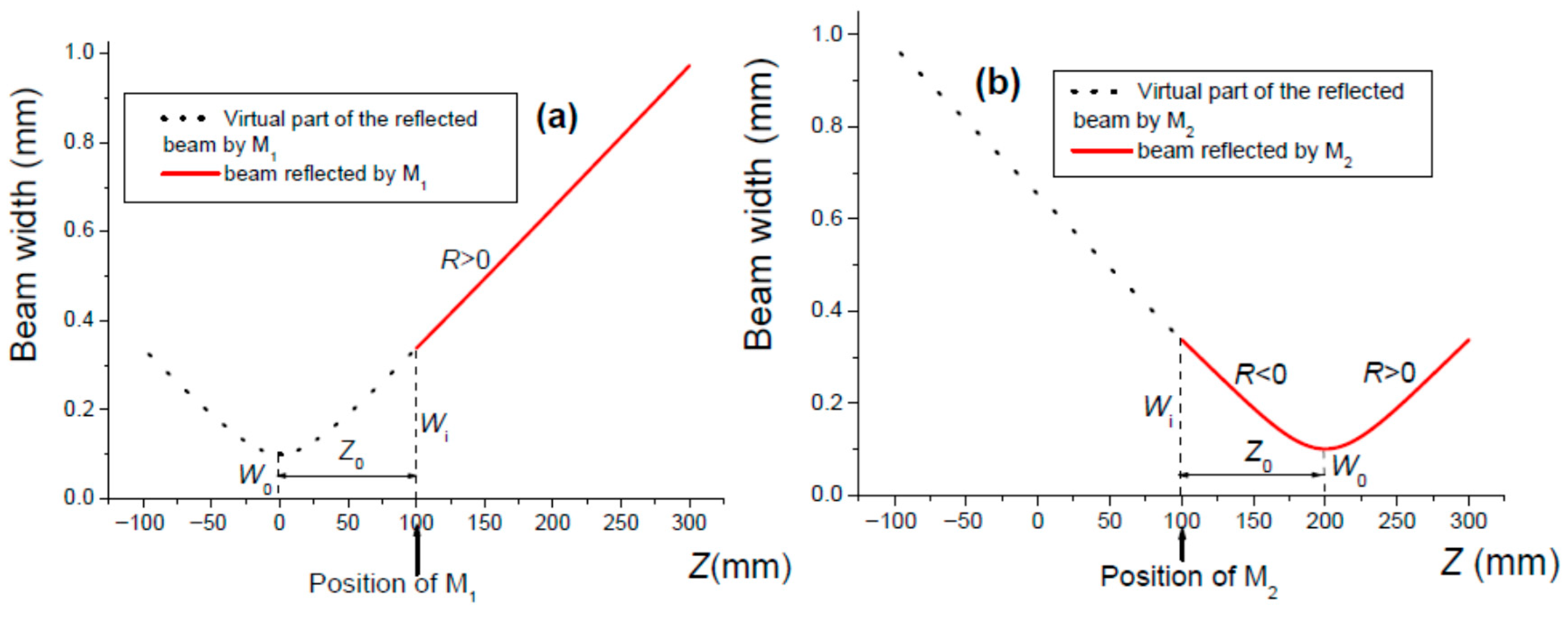
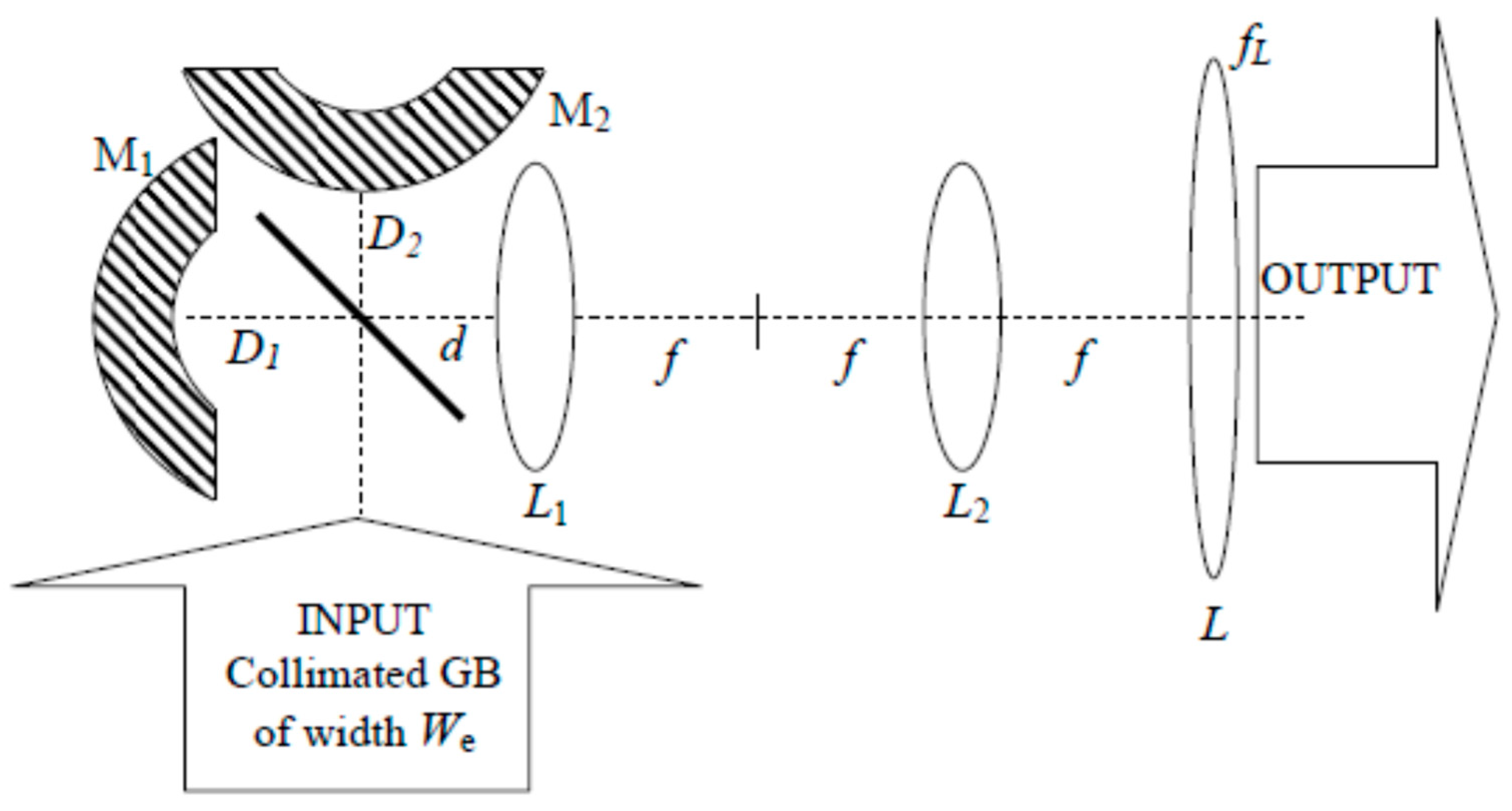
A careful examination of Figure A6 shows that there is no position for the output lens L where the two GBs have equal widths. This problem can be solved by using a 4f setup [71] serving as an optical relay for imaging the GBs existing in the plane of mirrors M₁ and M₂ into the plane of output lens L. The 4f setup uses two converging lenses of focal length $f_1$ and $f_2$ separated by a distance $D=f_1+f_2$. An usual case is a 4f setup made up of two identical lenses ($f_1=f_2=f$). This setup comprises an input plane positioned in the front focal plane of the first lens $L_1$, and an output plane localised at the back focal plane of the second lens $L_2$. The first lens achieves a first Fourier transform, while the second lens realises a second Fourier transform so that one gets in the front focal plane of lens $L_2$ of the 4f setup a reproduction of the field outstanding in the input plane. Consequently, the couple $\left\{W_e,+R_M\right\}$ ($\left\{W_e,-R_M\right\}$) on mirror M₁ (M₂) is transferred onto the output lens L by means of the 4f system as shown in Figure A7. By taking into account Equations (A10) and (A15), one obtains the field distribution $E_L(\rho )$ in the plane of lens L in Figure A7:

$$E_L(\rho )=2E_0\times \exp \left[-{\rho }^2/W_e^2\right]\times \cos \left\{2\pi K{\displaystyle \frac{{\rho }^2}{W_e^2}}\right\}$$

(A19)

As shown above, note that the dispersion of the Michelson interferometer used for reshaping a Gaussian beam has been reduced by setting the arm lengths to the same length, i.e., $D_1=D_2$. However, the wavelength dependence of $K$ is determined according to Equation (A10). This remaining dispersion is considered in Section 3.

Figure A7. The first lens L₁ of the 4f setup is located so that f = D₁ + d = D₂ + d. The output focusing lens L is positioned at the back focal plane of lens L₂.

Figure A7. The first lens L₁ of the 4f setup is located so that f = D₁ + d = D₂ + d. The output focusing lens L is positioned at the back focal plane of lens L₂.

References

- Arlt, J.; Padgett, M.J. Generation of a beam with a dark focus surrounded by regions of higher intensity: The optical bottle beam. Opt. Lett. 2000, 25, 191–193. [Google Scholar] [CrossRef] [Scilit]
- Xu, P.; He, X.; Wang, J.; Zhan, M. Trapping a single atom in a blue detuned optical bottle beam trap. Opt. Lett. 2010, 35, 2164–2166. [Google Scholar] [CrossRef] [Scilit]
- Khanom, F.; Mohamed, N.; Lopushenko, I.; Sdobnov, A.; Doronin, A.; Bykov, A.; Rafailov, E.; Meglinski, I. Twists through turbidity propagation of light carrying orbital angular momentum through a complex scattering medium. Sci. Rep. 2024, 14, 20662. [Google Scholar] [CrossRef] [Scilit]
- Protasov, C.E.; Gusarov, A.V. Modeling the effect of beam shaping at selective laser melting. Procedia IUTAM 2017, 23, 147–154. [Google Scholar] [CrossRef] [Scilit]
- Wang, J. Advances in communications using optical vortices. Photonics Res. 2016, 4, B14–B28. [Google Scholar] [CrossRef] [Scilit]
- Kumar, S.; Sharma, N. Emerging military applications of free space optical communication technology. J. Phys. Conf. Ser. 2022, 2161, 012011. [Google Scholar] [CrossRef] [Scilit]
- Li, Y.; Lai, L.; Rui, C.; Wang, L. Optimization of depletion focal spot in STED nanoscopy using amplitude manipulation. Opt. Commun. 2016, 372, 132–136. [Google Scholar] [CrossRef] [Scilit]
- Buratto, L.; Böhm, E. The use of the femtosecond laser in penetrating keratoplasty. Am. J. Ophthalmol. 2007, 143, 737–742. [Google Scholar] [CrossRef] [Scilit]
- Bulanov, S.S.; Brantov, A.; Bychenkov, V.Y.; Chvykov, V.; Kalinchenko, G.; Matsuka, T.; Rousseau, P.; Reed, S.; Yanovsky, V.; Litzenberg, D.W.; et al. Accelerating monoenergetic protons from ultrathin foils by flat-top laser pulses in the directed Coulomb explosion regime. Phys. Rev. E 2008, 78, 026412. [Google Scholar] [CrossRef] [Scilit] [PubMed]
- Karnakis, D.M.; Fieret, J.; Rumsby, P.T.; Gower, M.C. Microhole drilling using reshaped pulsed Gaussian beams. In Laser Beam Shaping II; SPIE: Bellingham, WA, USA, 2001; Volume 4443, pp. 150–158. [Google Scholar]
- Le, H.; Penchev, P.; Henrottin, A.; Bruneel, D.; Nasrollahi, V.; Ramos-de-Campos, J.A.; Dimov, S. Effects of top-hat laser beam processing and scanning strategies in laser micro-structuring. Micromachines 2020, 11, 221. [Google Scholar] [CrossRef] [Scilit]
- Boutu, W.; Ducousso, M.; Hergott, J.F.; Merdji, H. Overview on HHG high-flux sources. In Optical Technologies for Extreme-Ultraviolet and Soft X-Ray Coherent Sources; Springer Series in Optical Sciences; Springer: Berlin/Heidelberg, Germany, 2015; Volume 197, pp. 63–78. [Google Scholar]
- Siegman, A. Analysis of laser beam quality degradation caused by quartic phase aberrations. Appl. Opt. 1993, 32, 5893–5901. [Google Scholar] [CrossRef] [Scilit]
- Haddadi, S.; Bencheikh, A.; Aït Ameur, K. Thermal lens focal length statistics for end-pumped solid-state lasers excited with different beam shapes. Appl. Opt. 2025, 64, C33–C40. [Google Scholar] [CrossRef] [Scilit]
- Harfouche, A.; Boubaha, B.; Fromager, M.; Aït-Ameur, K. Comparison between interferometric and diffractive laser beam shaping. J. Opt. 2014, 16, 125712. [Google Scholar] [CrossRef] [Scilit]
- Giles, A.J.; Posthumus, J.H.; Thompson, M.R.; Frasinski, L.J.; Codling, K.; Langley, A.J.; Shaikh, W.; Taday, P.F. Interferometric shaping of femtosecond laser pulses. Opt. Commun. 1995, 118, 537–541. [Google Scholar] [CrossRef] [Scilit]
- Chiou, A.E.; Wang, W.; Sonek, G.I.; Hong, J.; Berns, M.W. Interferometric optical tweezers. Opt. Commun. 1997, 133, 7–10. [Google Scholar] [CrossRef] [Scilit]
- Passilly, N.; De Saint Denis, R.; Aït-Ameur, K.; Treussart, F.; Hierle, R.; Roch, J.F. Simple interferometric technique for generation of a radially polarised light beam. J. Opt. Soc. Am. A 2005, 22, 984–991. [Google Scholar] [CrossRef] [Scilit]
- Niziev, V.G.; Chang, R.S.; Nesterov, A.V. Generation of inhomogeneously polarized laser beams by use of a Sagnac interferometer. Appl. Opt. 2006, 45, 8393–8399. [Google Scholar] [CrossRef] [Scilit] [PubMed]
- Gao, K.; Xu, L.; Zheng, R.; Chen, G.; Zheng, H.; Ming, H. Flat-top laser beam generated by coherent beam combining of Gaussian lasers. Chin. Opt. Lett. 2010, 8, 45–47. [Google Scholar] [CrossRef] [Scilit]
- Takaoka, T.; Kawano, N.; Awatsuji, Y.; Kubota, T. Design of a reflective aspherical surface of a compact beam-shaping device. Opt. Rev. 2006, 13, 77–86. [Google Scholar] [CrossRef] [Scilit]
- Zhang, S. A simple bi-convex refractive laser beam shaper. J. Opt. A Pure Appl. Opt. 2007, 9, 945–950. [Google Scholar] [CrossRef] [Scilit]
- Laskin, A.; Laskin, V. Variable beam shaping with using the same field mapping refractive beam shaper. In Laser Resonators, Microresonators, and Beam Control XIV; SPIE: Bellingham, WA, USA, 2012; Volume 8236. [Google Scholar] [CrossRef] [Scilit]
- Laskin, A.; Laskin, V. Imaging techniques with refractive beam shaping optics. In Laser Beam Shaping XIII; SPIE: Bellingham, WA, USA, 2012; Volume 8490. [Google Scholar] [CrossRef] [Scilit]
- Duerr, F.; Thienpont, H. Refractive laser beam shaping by means of a functional differential equation based design approach. Opt. Express 2014, 22, 8001–8011. [Google Scholar] [CrossRef] [Scilit]
- Laskin, A.; Laskin, V.; Ostrun, A. Refractive beam shapers for optical systems of lasers. In Components and Packaging for Laser Systems; SPIE: Bellingham, WA, USA, 2015; Volume 9346. [Google Scholar] [CrossRef] [Scilit]
- Laskin, A.; Laskin, V.; Ostrun, A. Generation of doughnut spot for high-power laser technologies using refractive beam shaping. In High-Power Laser Materials Processing: Lasers, Beam Delivery, Diagnostics, and Applications IV; SPIE: Bellingham, WA, USA, 2015; Volume 9356. [Google Scholar] [CrossRef] [Scilit]
- Zhang, P.; Gong, S.; Mittra, R. Beam-shaping techniques based on generalized laws of refraction and reflexion. IEEE Trans. Antennas Propag. 2018, 66, 771–779. [Google Scholar] [CrossRef] [Scilit]
- Feng, Z.; Huang, L.; Gong, M.; Jin, G. Beam shaping system design using double freeform optical surfaces. Opt. Express 2013, 21, 14728–14735. [Google Scholar] [CrossRef] [Scilit] [PubMed]
- Johansson, M.; Bengtsson, J. Robust design method for highly efficient beam-shaping diffractive optical elements using an iterative-Fourier-transform algorithm with soft operations. J. Mod. Opt. 2000, 47, 1385–1398. [Google Scholar] [CrossRef] [Scilit]
- Turunen, J.; Pääkkönen, P.; Kuittinen, M.; Laakkonen, P.; Simonen, J.; Kajava, T.; Kaivola, M. Diffractive shaping of excimer laser beams. J. Mod. Opt. 2000, 47, 2467–2475. [Google Scholar] [CrossRef]
- Liu, J.S.; Taghizadeh, M.R. Iterative algorithm for the design of diffractive phase elements for laser beam shaping. Opt. Lett. 2002, 27, 1463–1465. [Google Scholar] [CrossRef] [Scilit] [PubMed]
- Jia, J.; Zhou, C.; Sun, X.; Liu, L. Superresolution laser beam shaping. Appl. Opt. 2004, 43, 2112–2117. [Google Scholar] [CrossRef] [Scilit]
- Grewell, D.A.; Benatar, A. Diffractive optics as beam-shaping elements for plastic laser welding. Opt. Eng. 2007, 46, 118001. [Google Scholar] [CrossRef] [Scilit]
- Qu, W.; Gu, H.; Tan, Q.; Jin, G. Precise design of two-dimensional diffractive optical element for beam shaping. Appl. Opt. 2015, 54, 6521–6525. [Google Scholar] [CrossRef] [Scilit]
- De Sio, L.; Roberts, D.E.; Liao, Z.; Hwang, J.; Tabiryan, N.; Steeves, D.M.; Kimball, B.R. Beam shaping diffractive wave plates. Appl. Opt. 2018, 57, A118–A121. [Google Scholar] [CrossRef] [Scilit]
- Dickey, F.M.; Holsqade, S.C. Laser Beam Shaping Applications, 2nd ed.; Taylor & Francis Group: London, UK, 2017. [Google Scholar]
- Dickey, F.M. Laser Beam Shaping, 2nd ed.; Taylor & Francis Group: London, UK, 2014. [Google Scholar]
- Häfner, T.; Strauβ, J.; Roider, C.; Heberle, J.; Schmidt, M. Tailored laser beam shaping for efficient and accurate microstructuring. Appl. Phys. A 2018, 124, 111. [Google Scholar] [CrossRef] [Scilit]
- Stiglbrunner, C.F. Diffractive optical elements for laser beam shaping and control in optical systems. In Optical Technologies for Telecommunications 2024; SPIE: Bellingham, WA, USA, 2024; Volume 13738. [Google Scholar] [CrossRef] [Scilit]
- Buske, P.; Hofmann, O.; Bonnhoff, A.; Stollenwerk, J.; Holly, C. High fidelity laser beam shaping using liquid crystal on silicon spatial light modulator as diffractive neural networks. Opt. Express 2024, 32, 7064–7078. [Google Scholar] [CrossRef] [Scilit]
- Rullière, C. Femtosecond Laser Pulses, 2nd ed.; Springer: Cham, Switzerland, 2005. [Google Scholar]
- Ko, T.H.; Adler, D.C.; Fujimoto, J.G.; Mamedov, D.; Prokhorov, V.; Shidlovski, V.; Yakubovich, S. Ultrahigh resolution optical coherence tomography imaging with a broadband superluminescent diode light source. Opt. Express 2004, 12, 2112–2119. [Google Scholar] [CrossRef] [Scilit]
- Gupta, A.K.; Meng, R.; Modi, Y.S.; Srinivasan, V.J. Imaging human macular pigments with visible light optical coherence tomography and superluminescent diodes. Opt. Lett. 2023, 48, 4737–4740. [Google Scholar] [CrossRef] [Scilit] [PubMed]
- Kafar, A.; Stanczyk, S.; Schiavon, D.; Suski, T.; Perlin, P. Review on optimization and current status of (Al, In) GaN superluminescent diodes. ECS J. Solid State Sci. Technol. 2019, 9, 015010. [Google Scholar] [CrossRef] [Scilit]
- Gupta, A.K.; Meng, R.; Duelk, M.; Wald, K.; Srinivasan, V.J. High resolution visible light OCT of the human retina with combined superluminescent diodes. Opt. Lett. 2025, 50, 4070–4073. [Google Scholar] [CrossRef] [Scilit]
- Genty, G.; Coen, S.; Dudley, J.M. Fiber supercontinuum sources. J. Opt. Soc. Am. B 2007, 24, 1771–1785. [Google Scholar] [CrossRef] [Scilit]
- Dudley, J.M.; Taylor, J.R. Supercontinuum Generation in Optical Fibers; Cambridge University: Cambridge, UK, 2010. [Google Scholar]
- Alfano, R.R. The Supercontinuum Laser Source; Springer: Cham, Switzerland, 2006. [Google Scholar]
- Singh, M.; Tervo, J.; Turunen, J. Broadband beam shaping with harmonic diffractive optics. Opt. Express 2014, 22, 22680–22688. [Google Scholar] [CrossRef] [Scilit] [PubMed]
- Perumal, L.; Forbes, A. Broaband structured light using digital micro-mirror devices (DMDs): A tutorial. J. Opt. 2023, 25, 074003. [Google Scholar] [CrossRef] [Scilit]
- Cerpentier, J.; Meuret, Y. Real-time, broadband beam shaping with programmable freeform topologies. J. Phys. Photonics 2026, 8, 015021. [Google Scholar] [CrossRef] [Scilit]
- Moulton, P.F. Spectroscopy and laser characteristics of Ti:Al2O3. J. Opt. Soc. Am. B 1986, 3, 125–133. [Google Scholar] [CrossRef] [Scilit]
- Morova, Y.; Simsek, I.; Sennaroglu, A. Continuous-ave 2.3 µm Tm3+:Lu2O3 ceramic laser with ultrabroad tenability between 1845 nm and 2328 nm. Opt. Lett. 2025, 50, 1220–1223. [Google Scholar] [CrossRef] [Scilit] [PubMed]
- Morova, Y.; Ardali, E.; Denker, B.; Galagan, B.; Sverchkov, S.; Sennaroglu, A. Broadly tunable continuous wave 2.3 µm Tm3+: Tellurite glass laser. Opt. Lett. 2023, 48, 4681–4684. [Google Scholar] [CrossRef] [Scilit] [PubMed]
- Boubaha, B.; Naidoo, D.; Godin, T.; Fromager, M.; Forbes, A.; Aït-Ameur, K. Spatial properties of coaxial coherent Gaussian beams. Appl. Opt. 2013, 52, 5766–5772. [Google Scholar] [CrossRef] [Scilit] [PubMed]
- Forbes, A.; Dudley, A.; McLaren, M. Creation and detection of optical modes with spatial light modulators. Adv. Opt. Photonics 2016, 8, 200–227. [Google Scholar] [CrossRef] [Scilit]
- Rosales-Guzman, C.; Forbes, A. Structured Light with Spatial Light Modulator; SPIE Press: Bellingham, WA, USA, 2024. [Google Scholar]
- Lazarev, G.; Chen, P.J.; Strauss, J.; Fontaine, N.; Forbes, A. Beyond the display: Phase-only liquid crystal on silicon devices and their applications in photonics. Opt. Express 2019, 27, 16206–16249. [Google Scholar] [CrossRef] [Scilit]
- De Saint Denis, R.; Passilly, N.; Laroche, M.; Mohammed-Brahim, T.; Aït-Ameur, K. Beam shaping longitudinal range of a binary diffractive element. Appl. Opt. 2006, 45, 8136–8141. [Google Scholar] [CrossRef] [Scilit]
- Kogelnik, H.; Li, T. Laser beams and resonators. Appl. Opt. 1966, 5, 1550–1567. [Google Scholar] [CrossRef] [Scilit]
- Sato, S. Applications of liquid crystals to variable-focusing lenses. Opt. Rev. 1999, 6, 471–485. [Google Scholar] [CrossRef] [Scilit]
- Ren, H.; Fan, Y.H.; Gauza, S.; Wu, S.T. Tunable-focus flat liquid crystal lens. Appl. Phys. Lett. 2004, 84, 4789–4791. [Google Scholar] [CrossRef] [Scilit]
- Wang, B.; Ye, M.; Sato, S. Lens of electrically controllable focal length made by a glass lens and liquid-crystal layers. Appl. Opt. 2004, 43, 3420–3425. [Google Scholar] [CrossRef] [Scilit]
- Ren, H.; Wu, S.T. Variable-focus liquid lens. Opt. Express 2007, 15, 5931–5936. [Google Scholar] [CrossRef] [Scilit] [PubMed]
- Boyko, O.; Planchon, T.A.; Mercère, P.; Valentin, C.; Balcou, P. Adaptive shaping of a focused intense laser beam into a doughnut mode. Opt. Commun. 2005, 246, 131–140. [Google Scholar] [CrossRef] [Scilit]
- Strelkov, V.V.; Mével, E.; Constant, E. Generation of isolated attosecond pulses by spatial shaping of a femtosecond laser beam. New J. Phys. 2008, 10, 083040. [Google Scholar] [CrossRef] [Scilit]
- Bouzid, O.; Haddadi, S.; Fromager, M.; Cagniot, E.; Ferria, K.; Forbes, A.; Ait-Ameur, K. Focusing anomalies with binary diffractive optical element. Appl. Opt. 2017, 56, 9735–9741. [Google Scholar] [CrossRef] [Scilit]
- Mahajan, V.N. Zernike circle polynomials and optical aberrations of system with circular pupils. Appl. Opt. 1994, 33, 8121–8123. [Google Scholar] [CrossRef] [Scilit]
- Forbes, A.; Dickey, F.; DeGama, M.; Du Plessis, A. Wavelength tunable laser beam shaping. Opt. Lett. 2012, 37, 49–51. [Google Scholar] [CrossRef] [Scilit] [PubMed]
- Saleh, B.E.A.; Teich, M.C. Fundamentals of Photonics, 2nd ed.; Wiley-Interscience: Hoboken, NJ, USA, 2007; Chapter 4. [Google Scholar]
Disclaimer/Publisher’s Note: The statements, opinions and data contained in all publications are solely those of the individual author(s) and contributor(s) and not of MDPI and/or the editor(s). MDPI and/or the editor(s) disclaim responsibility for any injury to people or property resulting from any ideas, methods, instructions or products referred to in the content. |
© 2026 by the authors. Licensee MDPI, Basel, Switzerland. This article is an open access article distributed under the terms and conditions of the Creative Commons Attribution (CC BY) license.