An Edge-Preserving Nonlinear Error Suppression Method for Fringe Projection Profilometry Based on Low-Pass Guided Filtering

Abstract

In fringe projection profilometry, phase accuracy is a key factor in determining the ultimate measurement precision. However, errors stemming from the nonlinear response of the projector and camera are introduced into the phase map, manifesting as periodic artifacts that seriously compromise measurement fidelity. Although traditional phase filtering can effectively mitigate these artifacts, it often introduces edge blurring and detail loss. To address this, we first establish models for both the nonlinear error and its propagation and then propose a novel phase filtering algorithm based on low-pass guided filtering. This method effectively suppresses nonlinear artifacts while preserving edges, thereby improving calibration and measurement accuracy without requiring additional hardware. Our algorithm enhances the traditional four-step phase-shifting method: in simulations, it reduces calibration error by 52.2% (from 0.1490 mm to 0.0712 mm), and measurement error by over 36.8% (from 0.0855 mm to 0.0559 mm); in real experiments, these reductions are 54.1% (from 0.1180 mm to 0.0875 mm) and more than 36.7% (from 0.0954 mm to 0.0604 mm), respectively. Experimental results show that our method achieves accuracy comparable to the eight-step phase-shifting method while preserving the efficiency of the four-step method, highlighting its significant practical value.

1. Introduction

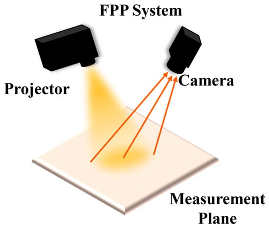
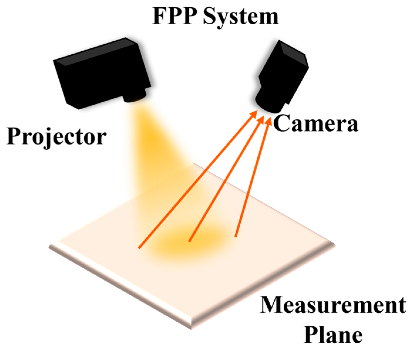
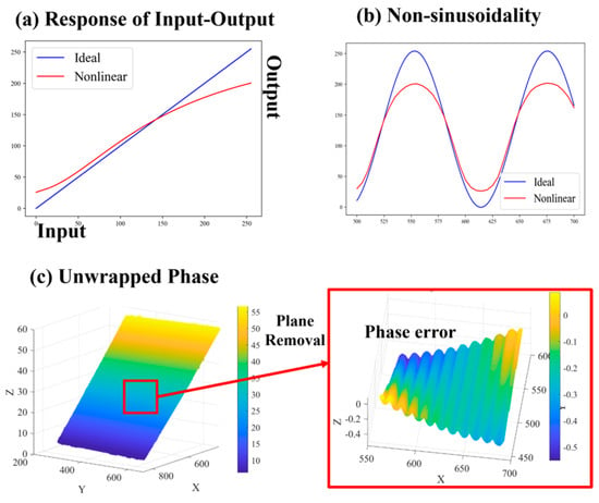
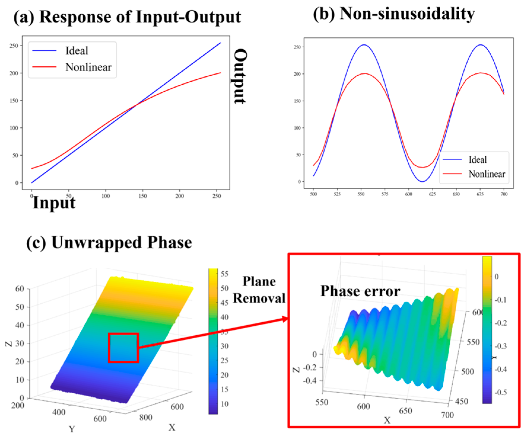
Fringe projection profilometry (FPP) has been widely used in industrial inspection [1], reverse engineering [2], face recognition [3], and virtual reality [4] due to its advantages of being non-contact, high-precision, and high-efficiency [5,6]. A typical fringe projection measurement system, composed of a projector and a camera (see Figure 1), recovers the three-dimensional information of an object by demodulating the sinusoidal fringe pattern deformed by the measured surface [7]. Therefore, phase accuracy is critical to the ultimate measurement precision of the system [8]. However, under practical measurement conditions, the nonlinear response of the projector and camera (as shown in Figure 2a) distorts the captured fringes [9,10], resulting in non-sinusoidal fringe patterns (as shown in Figure 2b) and consequently introducing periodic artifacts into the phase map (as shown in Figure 2c). As a primary factor affecting phase accuracy, nonlinear error can, in severe cases, corrupt the true phase information, compromising both calibration accuracy and the quality of three-dimensional reconstruction [11,12].

Figure 1. Schematic diagram of the fringe projection system.

Figure 2. Process of nonlinear error generation.

To address nonlinear errors, various methods have been proposed, categorized as active or passive based on their underlying mechanisms [13]: The former mitigates errors in situ, while the latter compensates ex post through processing algorithms.

• Active methods mainly focus on system calibration through gamma estimation. Li et al. [14] calibrated the system gamma using a white flat plate and incorporated it into three-step phase-shifting fringes for phase error compensation. Chen et al. [15] established an exponential fringe model that effectively suppresses phase errors without prior calibration. Yu et al. [16] leveraged the probability distribution function of the wrapped phase to estimate the system gamma from a single three-step phase-shifting pattern, boosting estimation efficiency. Baldo et al. [17] based on experimental analysis of the nonlinear response of a fringe projection measuring system, proposed a nonlinear correction method using high-order polynomials. However, existing active methods, which focus on optimizing the signal source, are often constrained by hardware conditions or require pre-calibration.
• Passive methods primarily include look-up tables (LUTs) [18], iterative algorithms [19], and statistical approaches [7]. Fu et al. [18] proposed a straightforward LUT-based method that pre-establishes a phase error look-up table for compensation, albeit with a relatively cumbersome construction process. For iterative algorithms, Xing et al. [19], realized error correction by constructing an error function and iterating coefficients based on phase pairs from fringes of different frequencies. Additionally, Wang et al. [7] adopted a statistical method using histogram equalization to correct distorted phases. Compared with active methods, passive methods offer greater flexibility. But the aforementioned methods tend to incur higher computational costs and are more susceptible to environmental factors such as background brightness, object color, and illumination conditions [20]. As an efficient post-processing technique for error mitigation, phase filtering [21,22] adapts to diverse scenarios through tunable parameters. Moreover, it effectively suppresses phase noise while maintaining measurement efficiency. However, traditional phase filtering algorithms often introduce image blur, which not only makes edge preservation a critical challenge but also leads to the loss of fine details during nonlinear error suppression, ultimately degrading the overall measurement accuracy [19]. To address the aforementioned issue, this paper first establishes models of nonlinear error and its propagation, thereby elucidating the mechanisms underlying error generation and transmission. On this basis, a nonlinear phase artifact suppression algorithm based on low-pass guided filtering is proposed. By integrating low-pass filtering’s noise-smoothing ability with guided filtering’s edge-preserving property, the algorithm removes nonlinear phase artifacts while preserving edges, without requiring additional projected patterns or extra hardware. To validate its effectiveness and superiority, the proposed method is evaluated in both simulation and real experiments. The evaluation focuses on three key aspects: edge-preserving performance, calibration accuracy, and 3D reconstruction quality. Comparative analyses are conducted against four-step phase shifting, eight-step phase shifting, and other well-established filtering techniques.

The remainder of this paper is structured as follows: Section 2 first outlines the basic principles and then establishes the models of nonlinear error and its propagation, providing the theoretical basis for subsequent error suppression; Section 3 details the proposed low-pass guided filtering algorithm; Section 4 validates the proposed method through simulations and real experiments, supported by qualitative and quantitative analyses; and finally Section 5 concludes the paper.

2. Theoretical Basis and Model Establishment

2.1. Basic Principle of FPP

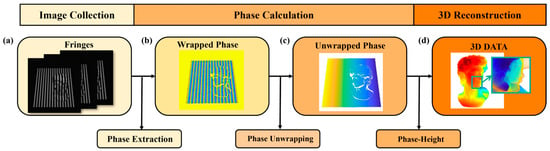
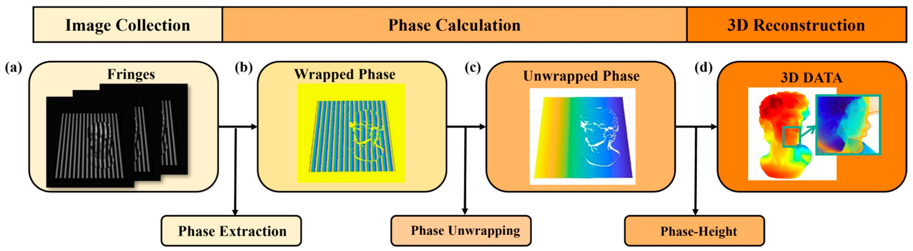
The measurement process of FPP primarily consists of image acquisition, phase calculation (including phase extraction and phase unwrapping), and three-dimensional (3D) reconstruction (see Figure 3).

Figure 3. Flowchart of fringe projection profilometry.

For the N-step phase shifting method, the intensity distribution of the n-th fringe pattern can be expressed as Equation (1):

$$I_n(x,y)=a(x,y)+b(x,y)\cos [\phi (x,y)+{\displaystyle \frac{2\pi n}{N}}](n=0,1,2,\dots ,N-1)$$

(1)

where I_n(x, y) is the intensity distribution of the n-th phase-shifted fringe pattern; a(x, y) represents the background intensity; b(x, y) represents the modulation amplitude; φ(x, y) represents the wrapped phase (range −π to π); N represents the number of phase shifting steps (typically N ≥ 3).

According to the least-squares principle, the wrapped phase φ(x, y) can be obtained from Equation (2):

$$\phi (x,y)=\arctan {\displaystyle \frac{{{\displaystyle \sum }}_{n=0}^{N-1}{I}_n(x,y)\sin \frac{2\pi n}{N}}{{{\displaystyle \sum }}_{n=0}^{N-1}{I}_n(x,y)\cos \frac{2\pi n}{N}}}(n=0,1,2,\dots ,N-1)$$

(2)

Since the principal phase value obtained from the arctangent function is truncated to the interval (−π, π], a phase unwrapping algorithm is required to recover the continuous absolute phase. Common phase unwrapping methods include the Gray code method [23], multi-frequency method [19], multi-wavelength method [24] and many others. With Gray-code method, the term of phase unwrapping is calculated by Equation (3):

$$k(x,y)=\sum _{i=0}^{n-1}{b}_i(x,y)\cdot 2^{n-1-i}$$

(3)

where b_i(x, y) is the i-th bit Gray-code value (0 or 1), and n is the number of encoding bits.

After that, the 3D coordinates can be calculated through the established phase-height mapping relationship. The polynomial model [25], one of the most commonly used calibration techniques, is shown as (4):

$$\begin{array}{c}x=f_x(u,v,p)={\displaystyle \sum _{i=0}^n}{\displaystyle \sum _{j=0}^n}{\displaystyle \sum _{k=0}^n}{a}_{ijk}{u}^i{v}^j{p}^k\\ y=f_y(u,v,p)={\displaystyle \sum _{i=0}^n}{\displaystyle \sum _{j=0}^n}{\displaystyle \sum _{k=0}^n}{b}_{ijk}{u}^i{v}^j{p}^k\\ z=f_z(u,v,p)={\displaystyle \sum _{i=0}^n}{\displaystyle \sum _{j=0}^n}{\displaystyle \sum _{k=0}^n}{c}_{ijk}{u}^i{v}^j{p}^k\end{array}$$

(4)

where (x, y, z) are the world coordinates, and (u, v, p) are the pixel coordinates and the corresponding phase value, a_ijk, b_ijk, and c_ijk are the polynomial coefficients for the corresponding terms, and n represents the degree of the polynomial fitting.

2.2. Modeling of Nonlinear Error

When nonlinearity exists in the system, the actual output intensity of fringe pattern is given by Equation (5):

$$I_n^{out}={(I_n^{in})}^{\gamma }={[a+b\cos (\phi +{\displaystyle \frac{2\pi n}{N}})]}^{\gamma }(n=0,1,2,\dots ,N-1)$$

(5)

where when γ ≠ 1, the input–output of the projector becomes nonlinear, resulting in distortion of the output waveform. Expanding the distorted waveform into a Fourier series, and noting that the function is even (so the sine coefficients are zero), we obtain Equation (6):

$$\begin{array}{l}{I}_n^{out}=a_0+{\displaystyle \sum _{k=1}^{\infty }}\left[a_k\cos n(\phi +{\displaystyle \frac{2\pi n}{N}})+b_n\sin (\phi +{\displaystyle \frac{2\pi n}{N}})\right]\\ ={\displaystyle \sum _{n=0}^{\infty }}{A}_n\cos (\phi +{\displaystyle \frac{2\pi n}{N}})\end{array}$$

(6)

Here, the coefficients $a_0$ and $a_k$ reflect the degree of waveform distortion caused by the nonlinearity, and their expressions are given as follows:

$$\begin{array}{l}{a}_k={\displaystyle \frac{2}{\pi }}{\int }_0^{\pi }{[a+b\cos \phi ]}^{\gamma }\cos [k(\phi +{\displaystyle \frac{2\pi n}{N}})]d\phi \\ ={\displaystyle \frac{2}{\pi }}{\int }_0^{\pi }{[a+b\cos \phi ]}^{\gamma }\cos (k\phi )d\phi ,k\ge 1\\ a_0={\displaystyle \frac{1}{\pi }}{\int }_0^{\pi }{[a+b\cos \phi ]}^{\gamma }d\phi \end{array}$$

Substituting the actual intensity expression into the phase calculation (2):

$$\begin{array}{l}{\phi }^{out}=\arctan \left({\displaystyle \frac{{\displaystyle \sum _{n=0}^{N-1}}{I}_n^{out}\sin \frac{2\pi n}{N}}{{\displaystyle \sum _{n=0}^{N-1}}{I}_n^{out}\cos \frac{2\pi n}{N}}}\right)\\ =\arctan \left({\displaystyle \frac{{\displaystyle \sum _{n=0}^{N-1}}\left(\frac{a_0}{2}+{\displaystyle \sum _{k=1}^{\infty }}{a}_k\cos \left(\phi +\sin \frac{2\pi n}{N}\right)\right)\sin \frac{2\pi n}{N}}{{\displaystyle \sum _{n=0}^{N-1}}\left(\frac{a_0}{2}+{\displaystyle \sum _{k=1}^{\infty }}{a}_k\cos \left(\phi +\sin \frac{2\pi n}{N}\right)\right)\cos \frac{2\pi n}{N}}}\right)\end{array}$$

(7)

Let the numerator be $S$ and the denominator be $C$. Based on the orthogonality of trigonometric functions, the integral of the corresponding term is nonzero only when $\left(k+1\right)$ or $\left(k−1\right)$ is an integer multiple of $N$. Thus:

$$\begin{array}{l}S={\displaystyle \frac{N}{2}}\left[a_1\sin \phi -{\displaystyle \sum _{m=1}^{\infty }}{a}_{mN-1}\sin ((mN-1)\phi )+{\displaystyle \sum _{m=1}^{\infty }}{a}_{mN+1}\sin ((mN+1)\phi )\right]\\ C={\displaystyle \frac{N}{2}}\left[a_1\cos \phi +{\displaystyle \sum _{m=1}^{\infty }}{a}_{mN-1}\cos ((mN-1)\phi )+{\displaystyle \sum _{m=1}^{\infty }}{a}_{mN+1}\cos ((mN+1)\phi )\right]\end{array}$$

(8)

Substituting into Equation (7) gives:

$${\phi }_e=\arctan \left({\displaystyle \frac{a_1\sin \phi +{\displaystyle \sum _{m=1}^{\infty }}{a}_{mN-1}\sin ((mN-1)\phi )-{\displaystyle \sum _{m=1}^{\infty }}{a}_{mN+1}\sin ((mN+1)\phi )}{a_1\cos \phi +{\displaystyle \sum _{m=1}^{\infty }}{a}_{mN-1}\cos ((mN-1)\phi )+{\displaystyle \sum _{m=1}^{\infty }}{a}_{mN+1}\cos ((mN+1)\phi )}}\right)$$

(9)

Let:

$$S_m=a_{mN-1}-a_{mN+1},C_m=a_{mN-1}+a_{mN+1}$$

(10)

Then we have:

$${\phi }_e=\arctan \left({\displaystyle \frac{{\displaystyle \sum _{m=1}^{\infty }{S}_m\sin (mN\phi )}}{a_1+{\displaystyle \sum _{m=1}^{\infty }{C}_m\cos (mN\phi )}}}\right)$$

(11)

Define the complex number $Z=C+iS$; its argument ${\varphi }_e$ is the measured phase. Considering the argument $\varphi (c,s)$ as a function of the real part $C$ and the imaginary part $S$, when small perturbations $\Delta C$ and $\Delta S$ exist in the real and imaginary parts, the argument variation is given by:

$$\Delta \phi \approx {\displaystyle \frac{C\Delta S-S\Delta C}{C^2+S^2}}$$

(12)

Given that the amplitudes of higher-order harmonics $a_k$ (k ≥ 2) are much smaller than the fundamental frequency amplitude $a_1$, when the real and imaginary parts undergo small perturbations $\Delta C$ and $\Delta S$, the argument variation $\Delta \varphi$ can be expressed as:

$$\Delta \phi \approx {\displaystyle \sum _{m=1}^{\infty }\frac{S_m}{a_1}}\sin (mN\phi )$$

(13)

2.3. Modeling of Error Propagation

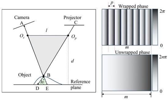
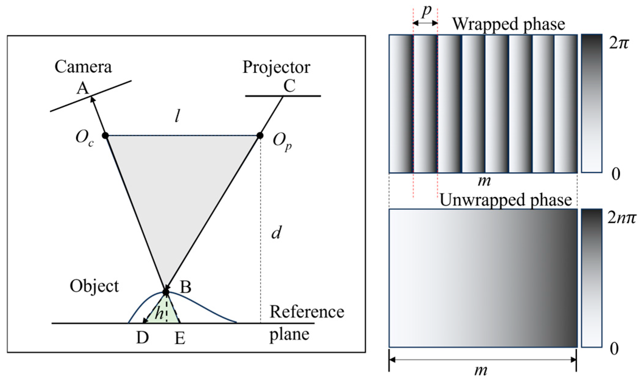
To analyze the impact of the phase error $\Delta \varphi$ on system calibration and measurement accuracy, this section establishes a corresponding error propagation model. To simplify the derivation, it is assumed that the optical centers of the projector and the camera are at the same height, and that the projection plane is parallel to the reference plane, as shown in Figure 4. Here, $O_c$ and $O_p$ denote the optical centers of the camera and projector, respectively; $B$ is an arbitrary point on the target surface; $A$ and $E$ are the intersections of line $O_{c}B$ with the camera image plane and the reference plane, respectively; $C$ and $D$ are the intersections of line $O_{p}B$ with the projector projection plane and the reference plane, respectively. Based on the principle of similar triangles, we obtain:

$$h={\displaystyle \frac{l_{DE}\cdot d}{l+l_{DE}}}$$

(14)

where $l$ represents the distance between the optical centers of the projector and the camera, $d$ is the perpendicular distance from the projector’s optical center to the reference plane, and $l_{DE}$ denotes the distance between points $D$ and $E$. When $l\gg l_{DE}$, this can be simplified to:

$$h\approx {\displaystyle \frac{l_{DE}\cdot d}{l}}$$

(15)

Figure 4. Schematic diagram of the FPP model.

Since the projection plane is parallel to the reference plane, let the physical length corresponding to the period of the sinusoidal fringe pattern (i.e., the phase period) on the actual reference plane be $p$, the length of the complete projection area be $m$, and the maximum value of the unwrapped phase be $2n\pi$. Then we have:

$$l_{DE}=p{\phi }_{DE}={\displaystyle \frac{m}{2n\pi }}{\phi }_{DE}$$

(16)

Substituting into Equation (15) yields:

$$h\approx {\displaystyle \frac{dp}{l}}{\phi }_{DE}={\displaystyle \frac{dm}{2n\pi l}}{\phi }_{DE}=k{\phi }_{DE}$$

(17)

where $k$ is the calibration coefficient. From this, the relationship between the phase error and the height error can be derived as:

$$\Delta h=k\Delta \phi$$

(18)

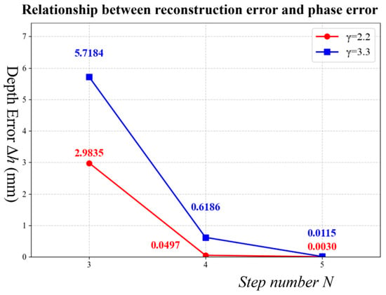
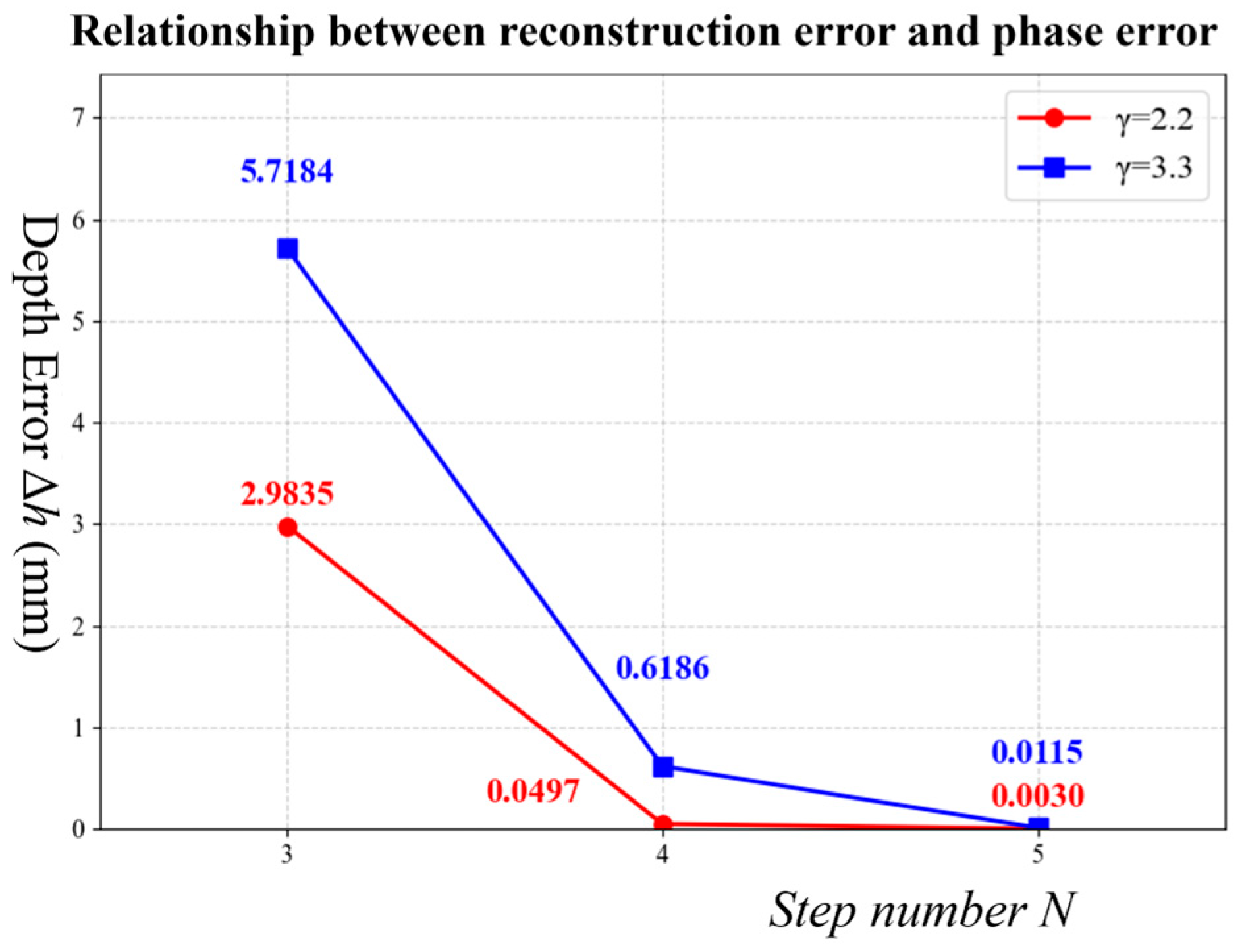
Under typical parameter settings: camera equivalent focal length $f=3000$, projection distance $d=1500\mathrm{mm}$, projection area length $m=100\mathrm{mm}$, number of phase periods $n=15$, system baseline length $l=80\mathrm{mm}$, and the camera-image-plane to measured-plane angle $\theta ={15}^{°}$, the calculated value is $k\approx 19.89\mathrm{mm}/\mathrm{rad}$. To assess the suppression of nonlinear errors under different phase-shifting steps $N$, we estimated the reconstruction errors for $N=3$, 4, and 5 at $\gamma =2.2$ and $3.3$. The results (Figure 5) show that the nonlinear error suppression capability increases with N.

Figure 5. Relationship between reconstruction error and phase error.

3. Principle of Low-Pass Guided Filtering for Nonlinear Error

To mitigate nonlinear errors in phase-shifting profilometry, this section presents the principle of low-pass guided filtering. First, phase filtering is analyzed using linear time-invariant (LTI) theory to establish harmonic suppression conditions. Then, a low-pass guided filtering algorithm is proposed, which overcomes the edge-blurring drawback of conventional low-pass filtering while retaining the edge-preserving advantage of standard guided filtering. Theoretical derivation and performance analysis follow.

3.1. Phase Filtering Algorithm

In phase shifting profilometry, the nonlinear response of the projector and camera can distort the sinusoidal fringe patterns, thereby introducing higher-order harmonic errors into the phase calculation. From Equation (13), the phase affected by nonlinear errors is given by:

$${\phi }_e=\phi +k\sin (N\phi )+\eta (\phi )$$

(19)

where ${\varphi }_e$ represents the measured phase with nonlinear errors, $\varphi$ is the ideal phase value, $k$ is an error coefficient independent of $\varphi$, and $N$ is the number of phase shift steps. The term $k\mathrm{s}\mathrm{i}\mathrm{n}\left(N\varphi \right)$ represents the dominant $N$-th harmonic component introduced by nonlinearity, while $\eta \left(\varphi \right)$ denotes the remaining higher-order harmonic components. To suppress the higher-order harmonic components introduced by the system’s nonlinear response, phase filtering can be applied.

Phase filtering is essentially a convolution operation in the phase domain. For a linear time-invariant (LTI) filter, this can be expressed as:

$$\begin{array}{l}{\phi }_{filtered}={\phi }_e\ast h(x)={\displaystyle {\int }_{-\infty }^{+\infty }{\phi }_e(\tau )}\cdot h\left(x-\tau \right)d\tau \\ =D\cdot {\phi }_e+M_1\cdot {{\phi }_e}^{\prime }+\dots \end{array}$$

(20)

where $h\left(x\right)$ is the impulse response of the filter. The frequency response $H\left(\omega \right)$ of an LTI filter determines the transmission characteristics for each frequency component. To achieve ideal distortion-free transmission of the phase while suppressing harmonic components, the filter must satisfy the following conditions: the magnitude response at the $N$-th harmonic frequency should be approximately zero, i.e., $H\left(N\right)\approx 0$; meanwhile, within the fundamental frequency and the effective signal band, the filter should meet the linear phase condition, i.e., $D=1$ and the phase response should be linear (constant group delay), thereby ensuring that the signal waveform remains undistorted. These conditions above indicate that a well-designed low-pass filter can meet the requirements for eliminating high-order harmonics.

3.2. Low-Pass Guided Filtering Algorithm

Although conventional low-pass filtering can effectively suppress high-order harmonics, it tends to blur edge details, which is detrimental to preserving surface topography details. Guided filtering [26] is widely adopted due to its edge-preserving property; however, its performance depends on the guide image. To combine the high-order harmonic suppression capability of low-pass filtering with the edge-preserving property of guided filtering, this paper proposes a low-pass guided filtering algorithm based on a low-pass guide image, and its effectiveness is theoretically derived as follows.

Guided filtering is based on a local linear model. Within a local window ${\omega }_k$ of radius $r$ defined in the guidance image $G$, the output image $Q$ is a linear transformation of the guidance image $G$:

$$Q_i=a_k{G}_i+b_k,\forall i\in {\omega }_k$$

(21)

where the coefficients $a_k$ and $b_k$ are obtained by minimizing the difference between the output $Q$ and the original input $I$. The corresponding cost function is:

$$E\left(a_k,b_k\right)={\displaystyle \sum _{i\in w_k}\left[{\left(a_k{G}_i+b_k-I_i\right)}^2+ϵa_k^2\right]}$$

(22)

Here, $ϵ$ is a regularization parameter that controls the magnitude of $a_k$, serving as a smoothing constraint. Minimizing the cost function yields the optimal coefficients within the window ${\omega }_k$:

$$a_k={\displaystyle \frac{Cov{(G,I)}_k}{Var{(G)}_k+ϵ}},b_k={\overline{I}}_k-a_k{\mu }_k$$

(23)

where ${\mu }_k$ and $\mathrm{Var}(G{)}_k$ are the mean and variance of the guidance image $G$ within the window ${\omega }_k$, respectively; $\mathrm{Cov}(G,I)$ represents the covariance within the window; and ${\overline{I}}_k$ is the mean of the original input image $I$ within the same window. The final output is obtained by averaging over multiple windows:

$$Q_i={\displaystyle \frac{1}{\left|{\omega }_i\right|}}{\displaystyle \sum _{k:i\in {\omega }_k}(a_k{G}_i+b_k)}={\overline{a}}_i{G}_i+{\overline{b}}_i$$

(24)

where ${\overline{a}}_i$ and ${\overline{b}}_i$ are the means of the coefficients $a_k$ and $b_k$ over all windows that contain pixel $i$.

Taking the low-pass filtering result of the original phase as the guidance image, let the original noisy phase image be $I=S+N$, where $S$ is the true signal (containing edges and details) and $N$ is the noise. After low-pass filtering, the local variance of the guidance image $G$ is significantly reduced: $\mathrm{Var}(G{)}_k\ll \mathrm{Var}(S{)}_k+\mathrm{Var}(N{)}_k$. Moreover, since the noise is suppressed, the local covariance approximately equals the signal variance: $\mathrm{Cov}(G,I{)}_k\approx \mathrm{Var}(S{)}_k$. Substituting into Equation (23) yields:

$$a_k={\displaystyle \frac{Var{(S)}_k}{Var{(S)}_k+ϵ}}$$

(25)

In edge regions, where $\mathrm{Var}(S{)}_k$ is large, $a_k\approx 1$, thus preserving the edges. In flat regions, where $\mathrm{Var}(S{)}_k\to 0$, $a_k\to 0$; in this case, the output is dominated by ${\overline{b}}_i$:$Q_i\approx {\overline{b}}_i\approx {\overline{I}}_i$, which effectively takes the mean of the input within the window, achieving strong smoothing. It can thus be seen that the proposed low-pass guided filtering combines the strong smoothing capability of low-pass filtering with the edge-preserving property of guided filtering, enabling effective suppression of nonlinear phase harmonics while preserving detailed surface information.

4. Experiment and Discussion

4.1. Experimental System and Design

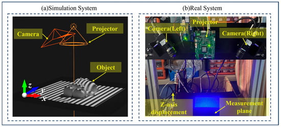
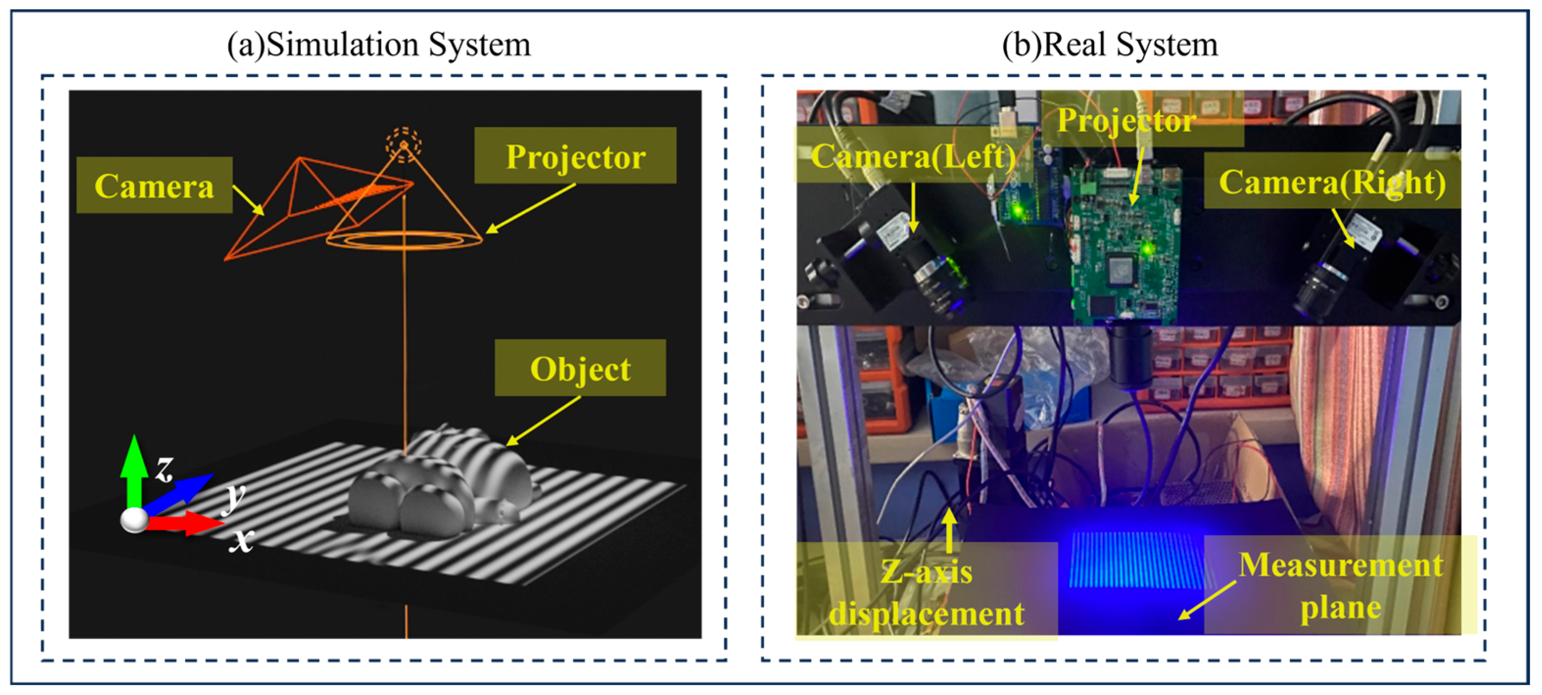
To validate the feasibility and effectiveness of the proposed algorithm, both simulation and real experiments were conducted in this study. The simulation experiment was built on the Blender 4.2.1 LTS platform, with the experimental system configuration shown in Figure 6a, which consists of a camera with a resolution of 960 × 1280 pixels (equipped with a 16 mm lens) and a projector employing a spotlight model. The real experimental system is shown in Figure 6b, and the detailed parameters are listed in Table 1.

Figure 6. Experimental System: (a) Simulation system and (b) Real system.

Table 1. Parameters of Real Experimental System.

Component	Parameter	Value
Camera	Model	MV-CA013-20GM (Hikvision, Hangzhou, China)
	Resolution	1280 × 1024
Lens	Model	MVL-HF1628M-6MPE (Hikvision, Hangzhou, China)
	Focal length	16 mm
Projector	Model	DLP4500 (Tianrui Video, Beijing, China)
	Resolution	1280 × 720
	Lens focal length	16 mm
Target	Manufacturing accuracy	±5 μm
Translation stage (Z-axis)	Positioning accuracy	800 nm
	Travel range	150 mm
Calibration volume		100 mm × 100 mm × 60 mm

To comprehensively evaluate the performance of the algorithm, the remainder of this section is organized as follows. Section 4.2 first verifies the edge-preserving capability of the algorithm. In Section 4.3, simulation experiments are conducted to qualitatively and quantitatively analyze the algorithm’s impact on calibration and measurement accuracy. Section 4.4 then presents real experiments to assess these effects in practical measurements.

4.2. Edge-Preserving Comparative Experiments

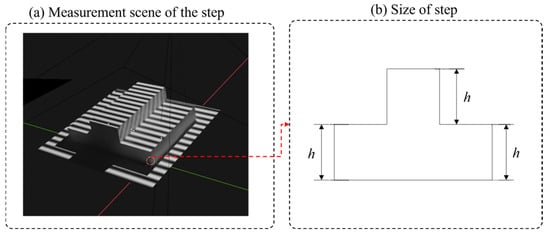
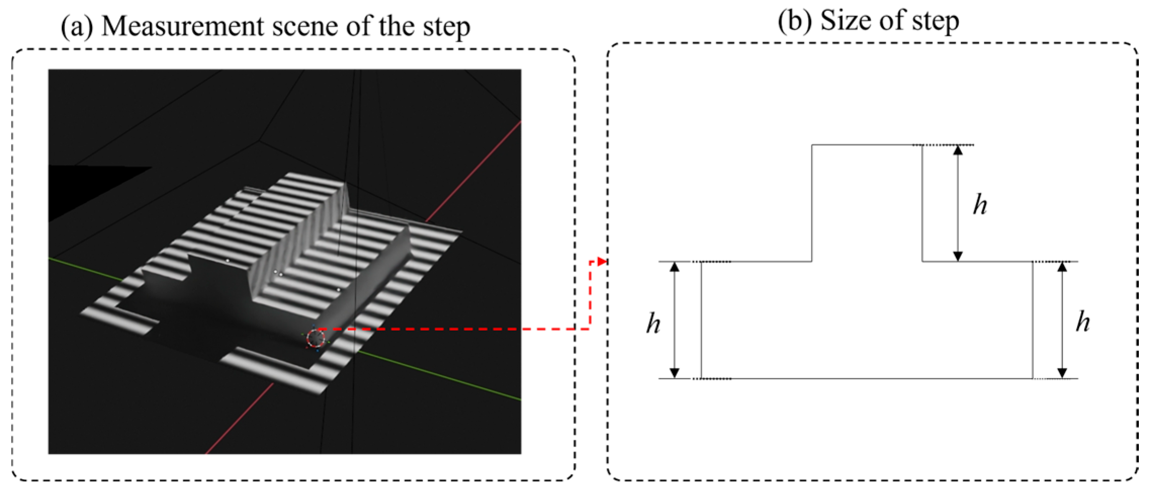
To verify the edge-preserving performance of the proposed low-pass guided filtering algorithm, a comparative experiment was designed in this section. A standard step target with a height of h = 20 mm was used as the measurement object (as shown in Figure 7), and the nonlinear coefficient of the system was set to $\gamma =2.2$. The edge-preserving capability of each method was evaluated by comparing the effectiveness of different filtering techniques in suppressing phase noise while preserving edge profiles. To objectively evaluate the edge-preserving performance of each algorithm, it was necessary to ensure that all methods were compared under similar noise suppression levels. Therefore, the parameters of each filtering method were calibrated as follows: a flat region on the upper surface of the step target was selected, and the standard deviation ${\sigma }_p$ of the phase values within this region was calculated as a metric for evaluating phase artifact severity. The standard deviation obtained from the eight-step phase shifting method in the same region was used as the target benchmark. The parameters of each filtering method were then adjusted so that the deviation from the benchmark value was controlled within $\pm 5\%$.

Figure 7. Bench Step.

The experimental groups were as follows:

• Group 1: Four-step phase-shifting method, serving as the baseline control group to evaluate the fundamental performance of phase demodulation.
• Group 2: Eight-step phase-shifting method, which exhibits strong nonlinear error suppression capability and high accuracy, used as the ground truth group for performance comparison.
• Group 3: Gaussian low-pass (Comparative method 1) [22] with standard deviation $\sigma =4$.
• Group 4: Butterworth low-pass filtering (Comparative method 2) [21] with order $n=2$.
• Group 5: Proposed method—low-pass guided filtering with regularization parameter $ϵ=0.01$ and window radius $r=3$.

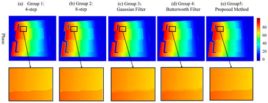
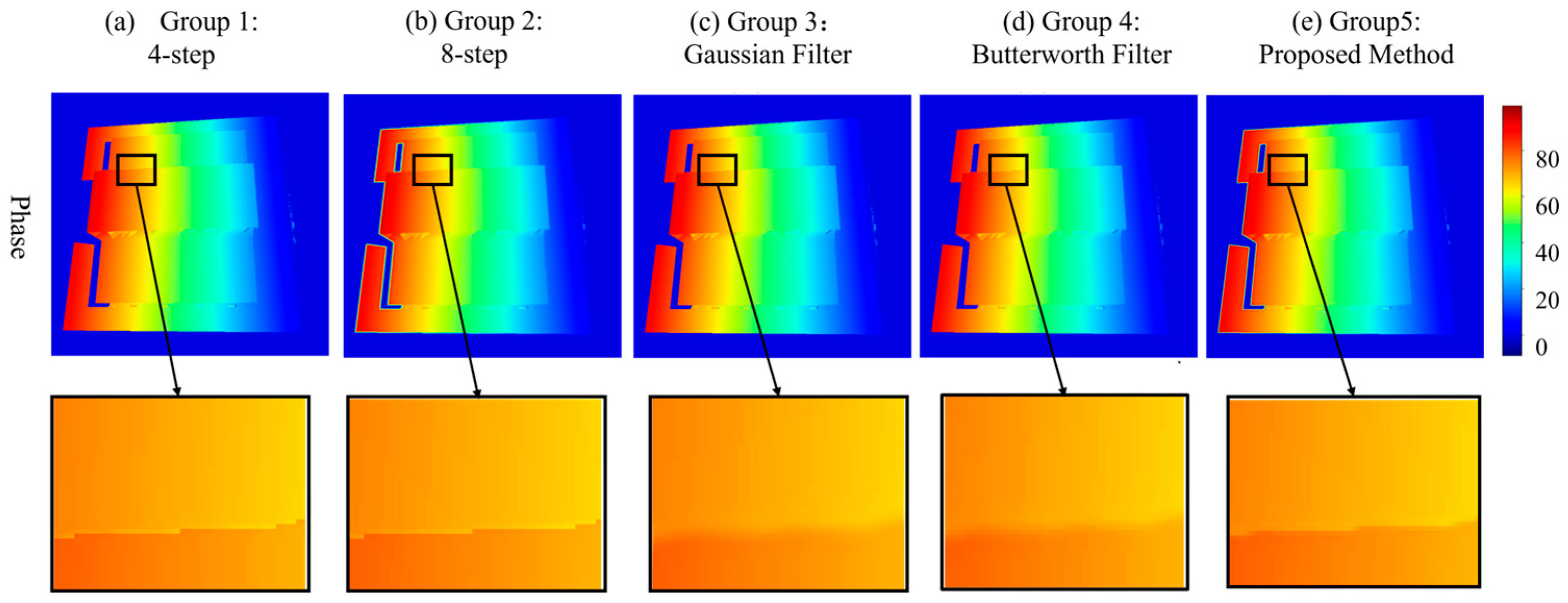
The experimental results are shown in Figure 8. Both the unfiltered four-step and eight-step phase shifting methods preserved sharp step edges, but nonlinear errors were present in the four-step results. A comparison of the edge-preserving performance of the three filtering methods reveals that both Gaussian low-pass guided filtering and Butterworth low-pass filtering caused noticeable edge blurring. In contrast, the proposed low-pass guided filtering method effectively suppressed phase noise while maintaining edge sharpness, demonstrating a significant improvement in edge preservation over the two comparative methods.

Figure 8. Comparison of edge-preserving performance.

To further quantitatively evaluate the edge-preserving effect of each filter, three metrics were introduced: the Edge Preservation Index (EPI) [27] Peak Signal-to-Noise Ratio (PSNR) [28], and Gradient Preservation Rate (GPR) [29]. The results are presented in Table 2. For EPI and GPR, values closer to 1 indicate better preservation of edge and gradient information, while higher PSNR values represent lower image distortion. As shown in the table, the proposed method achieves enhanced performance across all three metrics, with EPI, PSNR, and GPR reaching 0.9615, 39.18 dB, and 0.9850, respectively. Compared to Comparative Method 1, these represent improvements of 41.4% (from 0.6799 to 0.9615), 53.5% (from 25.52 to 39.18), and 9.4% (from 0.9000 to 0.9850), respectively; compared to Comparative Method 2, the improvements are 26.7% (from 0.7588 to 0.9615), 36.6% (from 28.68 to 39.18), and 5.8% (from 0.9308 to 0.9850), respectively. Moreover, the proposed method achieves results closely approaching those of the unfiltered four-step phase shifting method (0.9820, 42.24 dB, and 1.0000). These findings demonstrate that the proposed method effectively suppresses nonlinear errors while preserving edge and gradient information. Its edge-preserving performance is significantly superior to the two comparative methods, validating the effectiveness and superiority of the proposed algorithm.

Table 2. Quantitative evaluation results of edge preserving.

Method	EPI (→1)	PSNR (dB, ↑)	GPR (→1)
Four-step	0.9820	42.24	1.0000
Comparative method 1	0.6799	25.52	0.9000
Comparative method 2	0.7588	28.68	0.9308
Proposed method	0.9615	39.18	0.9850

Here, the closer the EPI and GPR values are to 1, the better the performance; and the larger the PSNR value, the better the performance.

4.3. Simulation Experiments

To validate the effectiveness of the proposed algorithm in suppressing nonlinear errors, simulation experiments were designed in this section for both quantitative and qualitative evaluation. The nonlinear coefficient of the system was set to $\gamma =2.2$. By comparing the denoising performance of different methods under similar edge-preserving levels, their impact on calibration accuracy and three-dimensional measurement results was analyzed. To ensure that all filtering methods were compared under similar edge-preserving levels, the parameters of each method were calibrated prior to the experiment. A distinct edge region within the image was selected, and the average gradient magnitude in this region was calculated. The gradient magnitude obtained from the eight-step phase shifting method in the same region was used as the benchmark. The parameters of each filtering method were then adjusted so that the deviation from the benchmark value was controlled within $\pm 5\%$. Five control groups were established in the experiment as follows:

• Group 1: Four-step phase shifting method, serving as the baseline control group before optimization.
• Group 2: Eight-step phase shifting method, used as a benchmark for performance comparison.
• Group 3: Gaussian low-pass filtering (Comparative method 1) with standard deviation $\sigma =1$.
• Group 4: Butterworth low-pass filtering (Comparative method 2) with order $n=4$.
• Group 5: Proposed method—low-pass guided filtering with regularization parameter $ϵ=0.01$ and window radius $r=3$.

The influence of each method on calibration accuracy was first evaluated with reprojection error. Based on five independent repeated experiments, the mean reprojection errors and standard deviations for each group are presented in Table 3. As shown in the table, the proposed method achieves a mean reprojection error of 0.0712 mm, which is not only 52.2% lower than that of the unoptimized four-step phase-shifting method (0.1490 mm) but also significantly outperforms Comparative methods 1 and 2. This error value is very close to that achieved by the high-precision eight-step phase-shifting method, and the standard deviation is comparable. These results indicate that the proposed method achieves high calibration accuracy similar to the eight-step method while maintaining good repeatability and stability.

Table 3. Reprojection errors (unit: mm).

Experimental Group	Mean Reprojection Error ± Standard Deviation
Group 1: Four-step phase shifting	0.1490 ± 0.0260
Group 2: Eight-step phase shifting	0.0655 ± 0.0135
Group 3: Comparative method 1	0.0893 ± 0.0323
Group 4: Comparative method 2	0.0782 ± 0.0224
Group 5: Proposed method	0.0712 ± 0.0120

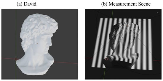
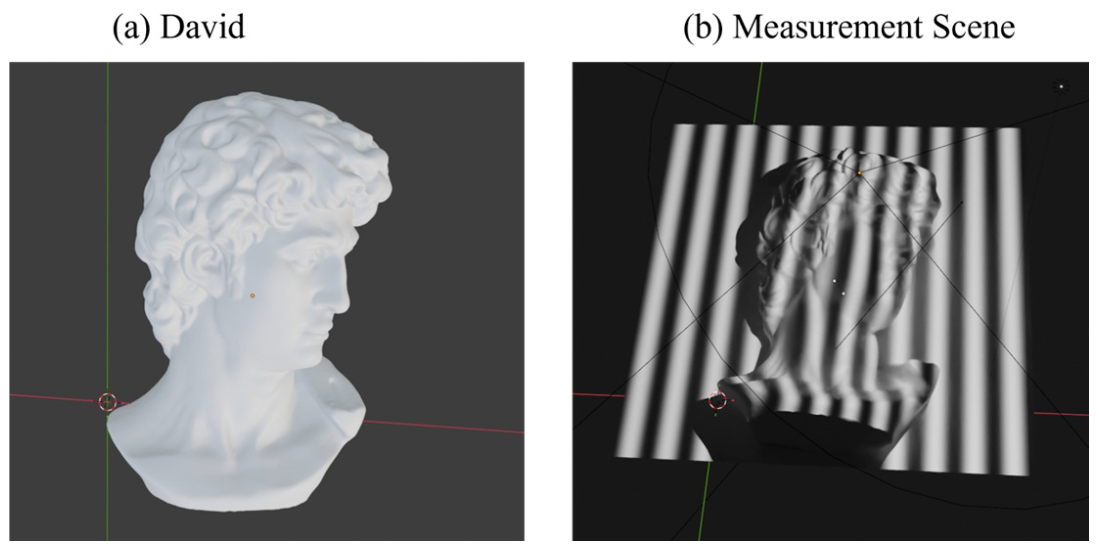
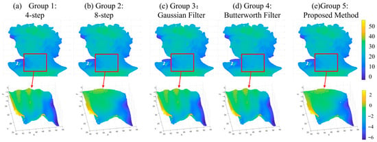
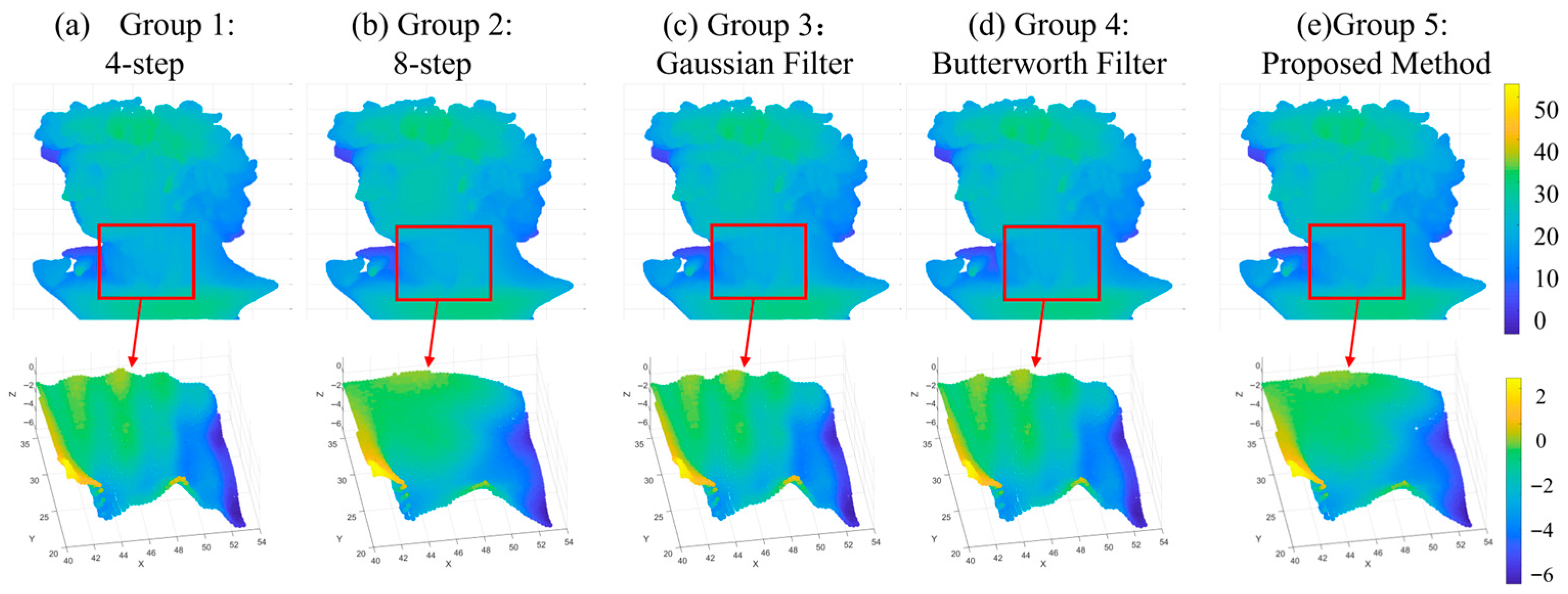
To further validate the performance of each method in actual surface measurement, a three-dimensional reconstruction of a David statue (Figure 9) was performed, with the results shown in Figure 10. In terms of reconstructed surface quality, the four-step phase shifting method exhibits limited capability in suppressing nonlinear errors, with noticeable wavy phase artifacts on the surface. Comparative methods 1 and 2 show some improvement, but artifacts are not entirely eliminated. The proposed method, however, effectively mitigates such artifacts, achieving a reconstructed surface quality close to that of the eight-step phase-shifting method.

Figure 9. Measurement object: David statue and (a) the object and (b) measurement scene.

Figure 10. Qualitative comparison of experimental results.

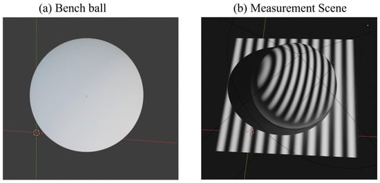
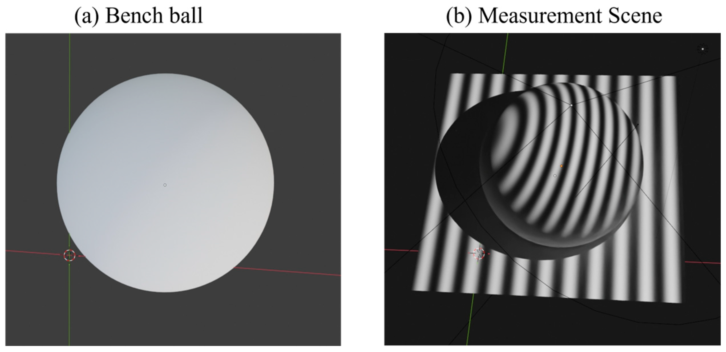
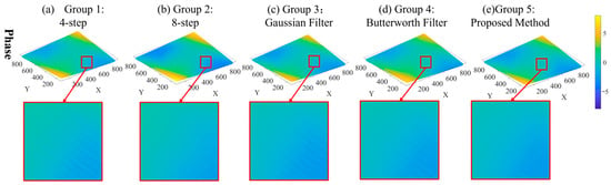
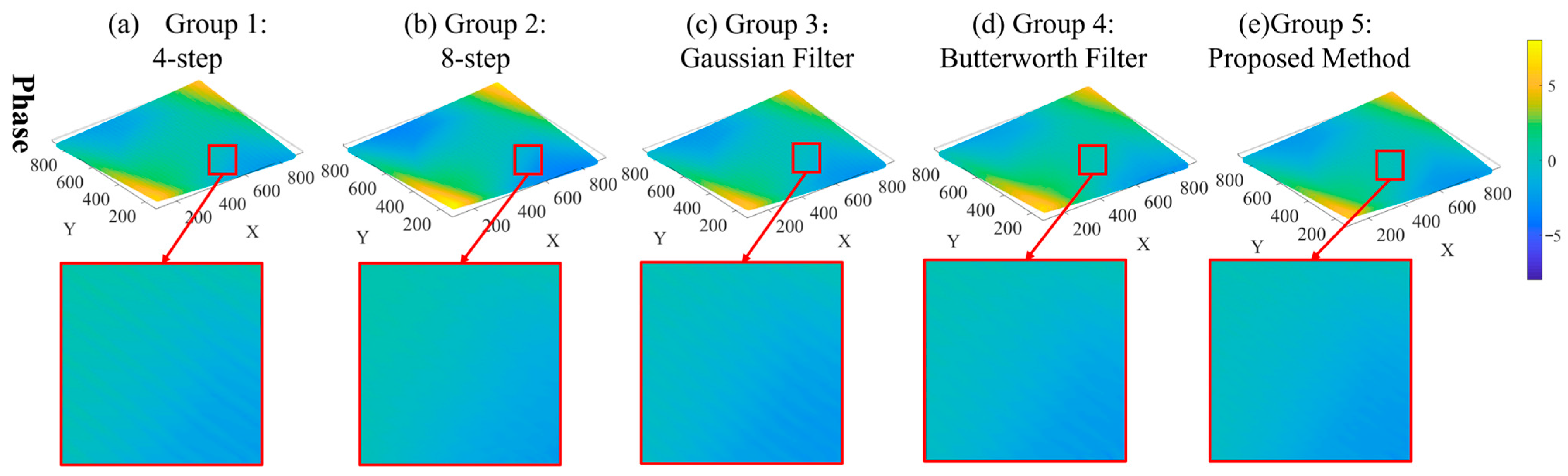
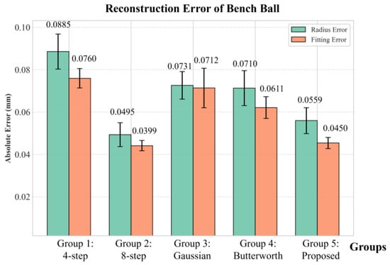
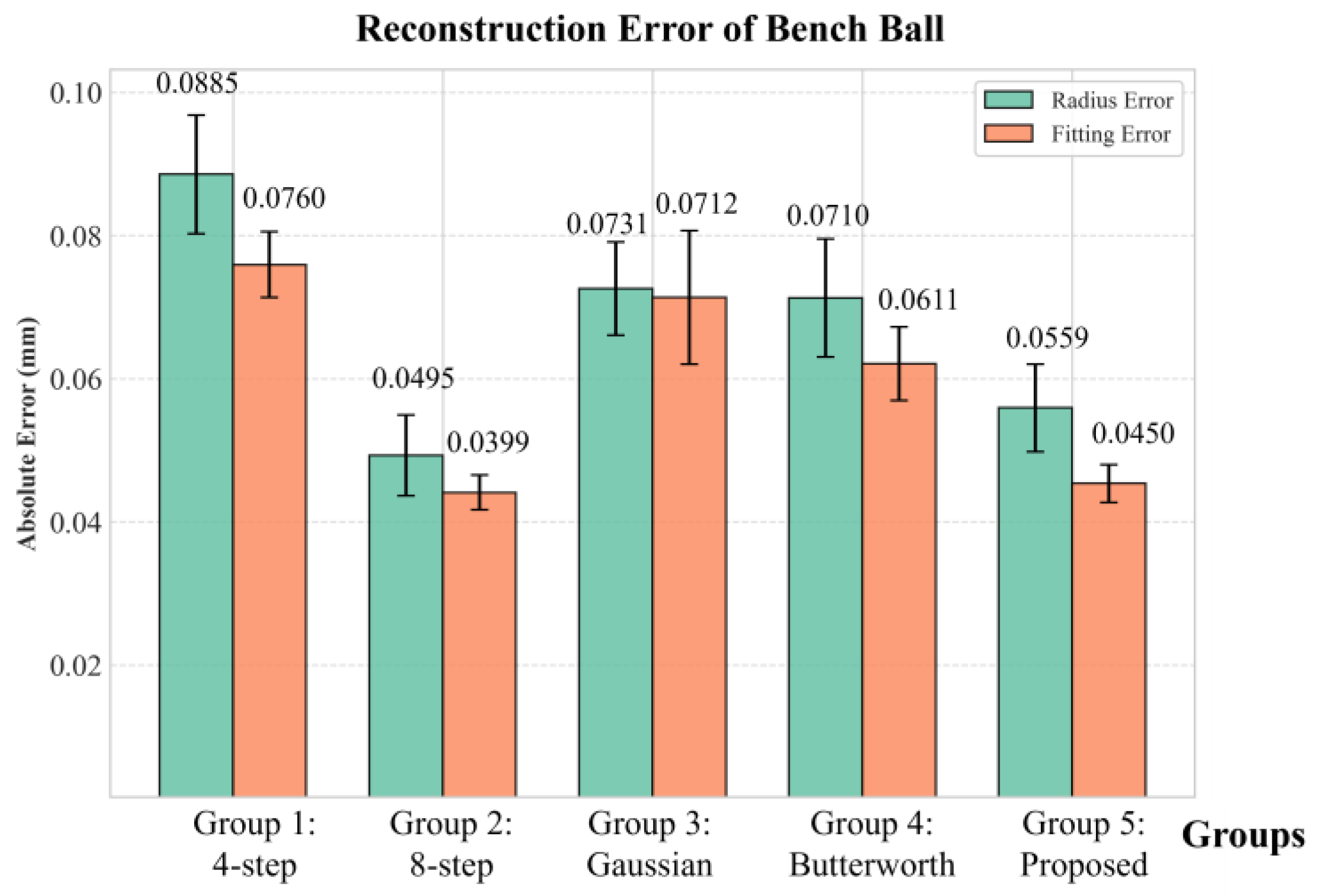
To quantitatively evaluate reconstruction accuracy, a standard sphere (diameter 50 mm) was used for accuracy validation, as shown in Figure 11. The phase calculation results are presented in Figure 12, from which it can be observed that the phase quality achieved by the proposed method is significantly better than that of Comparative methods 1 and 2 and is comparable to that of the eight-step phase-shifting method. Further statistical analysis of the reconstruction errors was conducted, with each group of experiments independently repeated five times. The results are shown in Figure 13. It can be seen that the proposed method exhibits enhanced performance in both error metrics. In terms of sphere diameter error, the proposed method (0.0559 mm) achieves a reduction of 36.8% compared to the four-step phase shifting method (0.0885 mm), significantly outperforming Comparative methods 1 and 2. Regarding sphere fitting error, the proposed method (0.0450 mm) achieves a reduction of 40.8% compared to the four-step method (0.0760 mm), also significantly surpassing the two comparative methods. Compared with the high-precision eight-step phase shifting method, both the sphere diameter error and sphere fitting error of the proposed method are very close, and the standard deviations are comparable. These results demonstrate that the proposed method achieves accuracy comparable to the eight-step phase-shifting method while maintaining good repeatability.

Figure 11. Measurement object: bench ball. (a) The object; (b) measurement scene.

Figure 12. Comparison of phase calculation results.

Figure 13. Comparison of three-dimensional reconstruction results.

4.4. Real Experiments

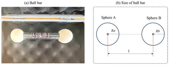
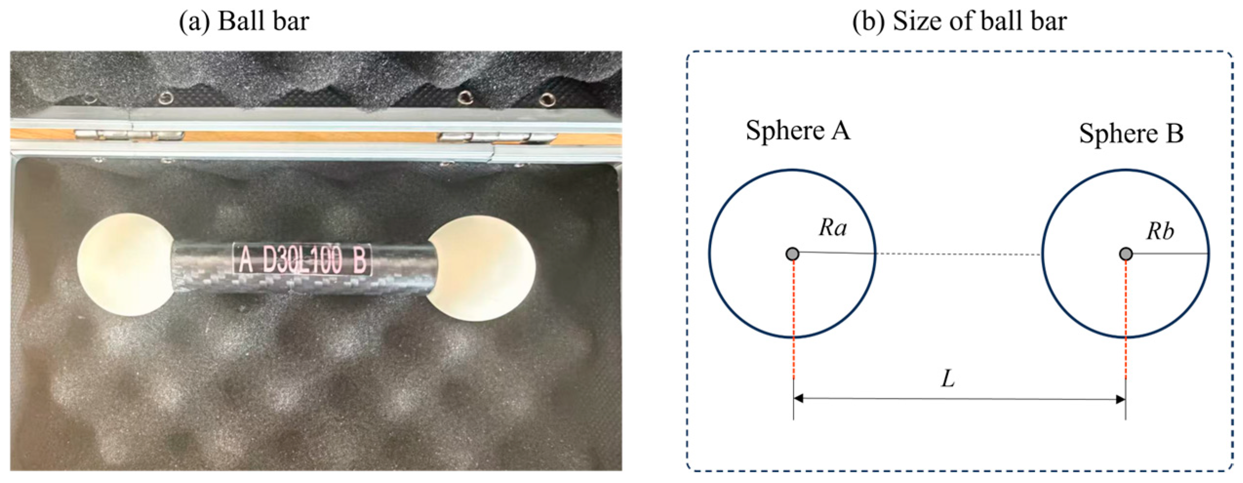
To validate the accuracy improvement achieved by the proposed algorithm in real experiments, this section first evaluates the calibration accuracy through reprojection error, followed by three-dimensional reconstruction validation using a standard sphere bar, along with qualitative and quantitative analyses. The standard sphere bar used in the experiment is shown in Figure 14, where the diameter of sphere A is 30.0087 mm, the diameter of sphere B is 30.0085 mm, and the center-to-center distance between the two spheres is 81.046 mm (expanded uncertainty $U=0.002$ mm with coverage factor $k=2$, coefficient of thermal expansion $\mathrm{CTE}=7\times {10}^{-6}$ /K, temperature $20\pm 0.5$ °C). After calibration, the nonlinear coefficient of the actual system was determined to be $\gamma \approx 2.2$, consistent with the simulation conditions. Based on this, the filter parameters were adopted from the calibration results in Section 4.3.

Figure 14. (a) Ball bar and (b) its size.

The experimental groups were configured as follows:

• Group 1: Four-step phase shifting method;
• Group 2: Eight-step phase shifting method;
• Group 3: Gaussian low-pass filtering (Comparative method 1) with standard deviation $\sigma =1$.
• Group 4: Butterworth low-pass filtering (Comparative method 2) with order $n=4$.
• Group 5: Proposed method—low-pass guided filtering with regularization parameter $ϵ=0.01$ and window radius $r=3$.

To verify the impact of each method on calibration results, a reprojection error analysis was first conducted. Based on five independent repeated experiments, the mean reprojection errors and standard deviations for each method are presented in Table 4. As can be observed, the reprojection error of the proposed method is significantly lower than that of the two comparative methods. Compared to the unoptimized four-step phase shifting method, the error of the proposed method is reduced by 54.1% (from 0.1180 mm to 0.0875 mm), while both the mean reprojection error and standard deviation are close to those of the eight-step phase shifting method. This indicates that the proposed method achieves high accuracy with better repeatability.

Table 4. Reprojection errors (unit: mm).

Experimental Group	Mean Reprojection Error ± Standard Deviation
Group 1: Four-step phase shifting	0.1180 ± 0.0222
Group 2: Eight-step phase shifting	0.0533 ± 0.0110
Group 3: Comparative method 1	0.0875 ± 0.0219
Group 4: Comparative method 2	0.0720 ± 0.0188
Group 5: Proposed method	0.0542 ± 0.0084

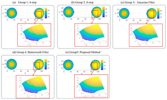
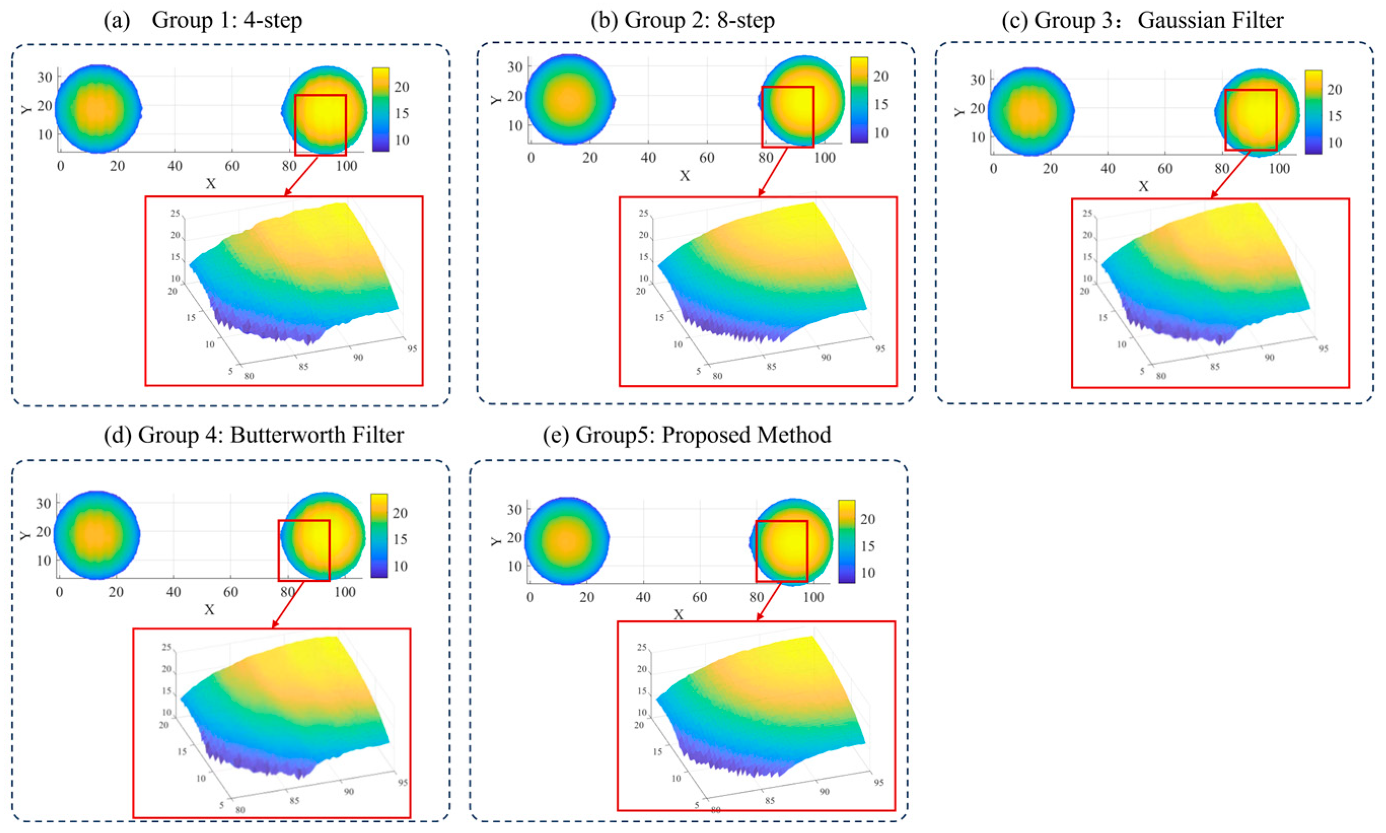
To further evaluate the performance of the proposed algorithm in actual three-dimensional reconstruction, the standard sphere bar was measured, with the results shown in Figure 15. It can be seen that the four-step phase shifting method exhibits limited capability in suppressing nonlinear errors, with noticeable artifacts remaining on the reconstructed surface. Comparative methods 1 and 2 show some improvement, but the surface is still not sufficiently smooth. In contrast, both the proposed method and the eight-step phase shifting method effectively suppress the nonlinearity-induced reconstruction errors, yielding smooth and flat reconstructed surfaces with visual quality highly close to that of the eight-step phase shifting method.

Figure 15. Reconstruction results.

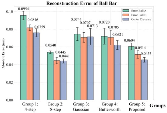
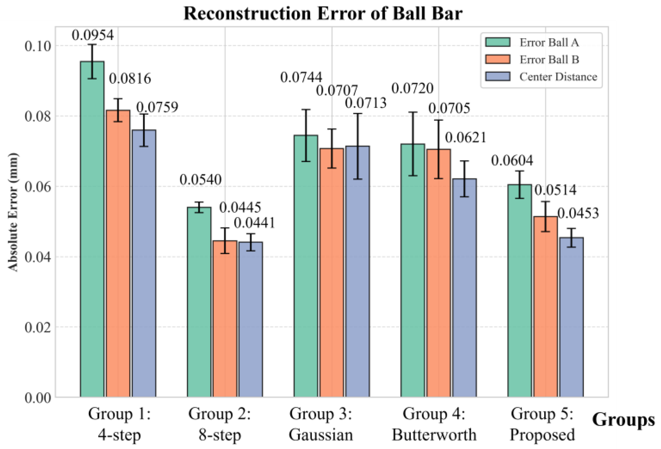
To further quantitatively evaluate the reconstruction accuracy, the following features were selected for statistical analysis: the diameter measurement error of sphere A and sphere B, and the error of the center-to-center distance between the two spheres. Each set of experiments was independently repeated five times under the same conditions to examine repeatability accuracy, with the results shown in Figure 16. From the experimental results, the proposed method achieves the following quantitative outcomes: the diameter error of sphere A is 0.0604 mm, the diameter error of sphere B is 0.0514 mm, and the center-to-center distance measurement error is 0.0453 mm. Compared with the four-step phase shifting method, these correspond to reductions of 36.7% (from 0.0954 mm to 0.0604 mm), 37.0% (from 0.0816 mm to 0.0514 mm), and 40.3% (from 0.0759 mm to 0.0453 mm), respectively. Moreover, the proposed method outperforms Comparative methods 1 and 2 in all three metrics. The results are very close to those of the high-precision eight-step phase shifting method, with the maximum difference being only 0.0069 mm (for sphere B diameter). In terms of repeatability, the standard deviation of the proposed method is comparable to that of the eight-step phase shifting method. These results demonstrate that the proposed method achieves accuracy and repeatability comparable to the eight-step phase shifting method.

Figure 16. Reconstruction errors of the sphere bar.

5. Conclusions

Fringe projection profilometry is widely regarded as one of the most promising techniques for three-dimensional measurement. Yet its measurement accuracy is frequently compromised by the nonlinear response of the system. To address this issue, this paper proposes a phase error suppression algorithm based on low-pass guided filtering. The proposed method integrates the smoothing capability of low-pass filtering with the edge-preserving property of guided filtering, effectively suppressing nonlinear phase artifacts while preserving edges without increasing the number of phase-shifting steps.

To evaluate the edge-preserving capability, we conducted comparative experiments in which the proposed algorithm demonstrated significantly superior edge preservation compared to traditional filtering methods under equivalent denoising performance. Following this, we conducted both simulation and experimental experiments, supported by qualitative and quantitative analyses. In simulations, compared with the conventional four-step phase-shifting method, the calibration reprojection error is reduced by 52.2% (from 0.1490 mm to 0.0712 mm), and the measurement accuracy is enhanced by over 36.8% (from 0.0855 mm to 0.0559 mm). In real experiments, the calibration reprojection error is reduced by 54.1% (from 0.1180 mm to 0.0875 mm), and the measurement accuracy is improved by over 36.7%. Both simulation and experimental results demonstrate that, built upon the conventional four-step method, our optimized algorithm achieves performance comparable to that of the eight-step phase-shifting method. This work provides an effective technical solution for achieving high-precision and high-efficiency fringe projection profilometry. In addition, the proposed algorithm is also applicable to improving the accuracy of other small-step phase-shifting methods (e.g., three-step and five-step phase shifting), which inherently have limited suppression capability against system nonlinearity due to the small number of steps.

References

- Yuan, H.; Li, Y.; Zhao, J.; Zhang, L.; Li, W.; Huang, Y.; Gao, X.; Xie, Q. An Adaptive Fringe Projection Method for 3D Measurement with High-Reflective Surfaces. Opt. Laser Technol. 2024, 170, 110062. [Google Scholar] [CrossRef] [Scilit]
- Ding, D.; Sun, J. 3-D Shape Measurement of Translucent Objects Based on Fringe Projection. IEEE Sens. J. 2023, 24, 3172–3179. [Google Scholar] [CrossRef] [Scilit]
- Guo, Y.; You, Z.; Lv, K.; Xiong, W.; You, D. High Accuracy, Compact 3D Face Imaging Method Based on Translational and Online-Switchable Phase-Shifting Fringe Projection. Opt. Express 2024, 32, 5671. [Google Scholar] [CrossRef] [Scilit]
- Shen, M.; Luo, J.; Chen, F.; Zhang, H.; Li, Y. Accurate Capture and Display of Real-World Three-Dimensional Scene Using Fringe Projection and Deep-Learning. Opt. Commun. 2026, 607, 132963. [Google Scholar] [CrossRef] [Scilit]
- Jakob, W. Real Time Structured Light and Applications. Ph.D. Thesis, Technical University of Denmark, Lyngby, Denmark, 2016. [Google Scholar]
- Liu, H.; Yan, N.; Shao, B.; Yuan, S.; Zhang, X. Deep Learning in Fringe Projection: A Review. Neurocomputing 2024, 581, 127493. [Google Scholar] [CrossRef] [Scilit]
- Wang, Y.; Cai, J.; Zhang, D.; Chen, X.; Wang, Y. Nonlinear Correction for Fringe Projection Profilometry with Shifted-Phase Histogram Equalization. IEEE Trans. Instrum. Meas. 2022, 71, 5005509. [Google Scholar] [CrossRef] [Scilit]
- Liu, H.; Zhang, X. A Deep Learning Approach for Small-Step High-Precision Phase Calculation in Fringe Projection: Integrating Phase Unwrapping and Compound Error Correction. Meas. J. Int. Meas. Confed. 2025, 256, 118480. [Google Scholar] [CrossRef] [Scilit]
- Kamagara, A.; Wang, X.; Li, S. Nonlinear Gamma Correction via Normed Bicoherence Minimization in Optical Fringe Projection Metrology. Opt. Eng. 2018, 57, 034107. [Google Scholar] [CrossRef] [Scilit]
- Gorthi, S.S.; Rastogi, P. Fringe Projection Techniques: Whither We Are? Opt. Lasers Eng. 2010, 48, 133–140. [Google Scholar] [CrossRef] [Scilit]
- Eiríksson, E.R.; Wilm, J.; Pedersen, D.B.; Aanaes, H. Precision and Accuracy Parameters in Structured Light 3-D Scanning. ISPRS-Int. Arch. Photogramm. Remote. Sens. Spat. Inf. Sci. 2016, XL-5/W8, 7–15. [Google Scholar] [CrossRef] [Scilit]
- Zheng, Y.; Duan, M.; Zhang, R.; Fan, X.; Jin, Y.; Zheng, J. Nonlinear Error Self-Correction for Fringe Projection Profilometry with Minimum Phase Probability Variance. Opt. Laser Technol. 2024, 174, 110658. [Google Scholar] [CrossRef] [Scilit]
- Jin, H.; Zhang, M.; Zhou, G.; Xiao, X.; Zhu, Y. Phase Error Restraint Method for Fringe Projection Measurement System. Laser Optoelectron. Prog. 2021, 58, 353–361. [Google Scholar]
- Li, Z.; Li, Y. Gamma-Distorted Fringe Image Modeling and Accurate Gamma Correction for Fast Phase Measuring Profilometry. Opt. Lett. 2011, 36, 154–156. [Google Scholar] [CrossRef] [Scilit] [PubMed]
- Chen, C.; Gao, N.; Wang, X.; Zhang, Z.; Gao, F.; Jiang, X. Generic Exponential Fringe Model for Alleviating Phase Error in Phase Measuring Profilometry. Opt. Lasers Eng. 2018, 110, 179–185. [Google Scholar] [CrossRef] [Scilit]
- Yu, X.; Liu, Y.; Liu, N.; Fan, M.; Su, X. Flexible Gamma Calculation Algorithm Based on Probability Distribution Function in Digital Fringe Projection System. Opt. Express 2019, 27, 32047–32057. [Google Scholar] [CrossRef] [Scilit] [PubMed]
- Baldo, C.; Sinico, M.; Dewulf, W. Experimental Investigation of the Nonlinear Response of a Research-Oriented Fringe Projection Measuring System. In Proceedings of the Special Interest Conference on Advancing Precision in Additive Manufacturing, Berlin, Germany, 6–9 October 2025; pp. 124–127. [Google Scholar]
- Fu, Y.; Wang, Z.; Jiang, G.; Yang, J. A Novel Three-Dimensional Shape Measurement Method Based on a Look-up Table. Optik 2014, 125, 1804–1808. [Google Scholar] [CrossRef] [Scilit]
- Xing, S.; Guo, H. Correction of Projector Nonlinearity in Multi-Frequency Phase-Shifting Fringe Projection Profilometry. Opt. Express 2018, 26, 16277–16291. [Google Scholar] [CrossRef] [Scilit] [PubMed]
- Li, W.-S. Application of Improved Phase-Measuring Profilometry in Nonconstant Environmental Light. Opt. Eng. 2001, 40, 478. [Google Scholar] [CrossRef] [Scilit]
- Wang, J.; Yang, Y. High Dynamic Range 3D Measurement Based on the Butterworth Low-Pass Filter and Hilbert Transform. J. Opt. Soc. Am. B 2023, 41, 197–207. [Google Scholar] [CrossRef] [Scilit]
- Lü, F.; Xing, S.; Guo, H. Self-Correction of Projector Nonlinearity in Phase-Shifting Fringe Projection Profilometry. Appl. Opt. 2017, 56, 7204–7216. [Google Scholar] [CrossRef] [Scilit]
- Yin, W.; Chen, Q.; Feng, S.; Tao, T.; Huang, L.; Trusiak, M.; Asundi, A.; Zuo, C. Temporal Phase Unwrapping Using Deep Learning. Sci. Rep. 2019, 9, 20175. [Google Scholar] [CrossRef] [Scilit] [PubMed]
- Zuo, C.; Huang, L.; Zhang, M.; Chen, Q.; Asundi, A. Temporal Phase Unwrapping Algorithms for Fringe Projection Profilometry: A Comparative Review. Opt. Lasers Eng. 2016, 85, 84–103. [Google Scholar] [CrossRef] [Scilit]
- Pei, X.; Liu, J.; Yang, Y.; Ren, M.; Zhu, L. Phase-to-Coordinates Calibration for Fringe Projection Profilometry Using Gaussian Process Regression. IEEE Trans. Instrum. Meas. 2022, 71, 5008112. [Google Scholar] [CrossRef] [Scilit]
- Zhu, S.; Yu, Z. Self-guided Filter for Image Denoising. IET Image Process. 2020, 14, 2561–2566. [Google Scholar] [CrossRef] [Scilit]
- Joseph, J.; Jayaraman, S.; Periyasamy, R.; Renuka, S. An Edge Preservation Index for Evaluating Nonlinear Spatial Restoration in MR Images. Curr. Med. Imaging Rev. 2017, 13, 58–65. [Google Scholar] [CrossRef] [Scilit]
- Chen, C.-Y.; Chen, C.-H.; Chen, C.-H.; Lin, K.-P. An Automatic Filtering Convergence Method for Iterative Impulse Noise Filters Based on PSNR Checking and Filtered Pixels Detection. Expert Syst. Appl. 2016, 63, 198–207. [Google Scholar] [CrossRef] [Scilit]
- Ma, X.; Hu, H.; Wu, P. A No-Reference Edge-Preservation Assessment Index for SAR Image Filters under a Bayesian Framework Based on the Ratio Gradient. Remote Sens. 2022, 14, 856. [Google Scholar] [CrossRef] [Scilit]
Disclaimer/Publisher’s Note: The statements, opinions and data contained in all publications are solely those of the individual author(s) and contributor(s) and not of MDPI and/or the editor(s). MDPI and/or the editor(s) disclaim responsibility for any injury to people or property resulting from any ideas, methods, instructions or products referred to in the content. |
© 2026 by the authors. Licensee MDPI, Basel, Switzerland. This article is an open access article distributed under the terms and conditions of the Creative Commons Attribution (CC BY) license.