


Abstract
As a core technology in 3D measurement, laser stripe center extraction is widely applied in industrial inspection, robot navigation, and biomedicine. However, traditional methods struggle to balance denoising effectiveness and positioning accuracy when handling complex noise and non-uniform width stripes. To address this bottleneck, this paper proposes a denoising-adaptive weighted average width stripe center extraction algorithm based on an improved Hessian Matrix, integrating deep learning with traditional image processing for high-precision extraction. A U-Net++ denoising network with a spatial attention module is designed to focus on stripe regions, supplemented by a distance-aware mechanism that dynamically adjusts denoising intensity based on pixel-stripe distance. For center extraction, an improved Hessian Matrix algorithm is proposed, incorporating a curvature-adaptive FIR filter and adaptive weighted average width calculation to adapt to stripe morphology changes. Experimental results show the algorithm outperforms comparative methods, achieving 35.26 dB (PSNR), 0.962 (SSIM), and 6.14 (RMSE) in denoising. Under 200 μs, 500 μs, 1000 μs, and 1500 μs exposure conditions, the absolute radius errors are reduced to 0.2052 mm, 0.1743 mm, 0.0268 mm, and 0.0281 mm, respectively, verifying its reliability and stability in practical applications.
1. Introduction
Laser stripe centerline extraction is a core fundamental technology in the fields of computer vision, precision measurement, and industrial inspection. Its extraction accuracy directly determines the reliability and precision of subsequent tasks such as 3D reconstruction, target contour measurement, and component dimension inspection. This technology plays an irreplaceable role in scenarios including form and position tolerance inspection of industrial mechanical parts, 3D environmental perception and path planning for robots, and microstructure measurement of biomedical tissue samples. However, disturbed by factors such as ambient light noise, surface reflection of measured objects, and optical distortion of equipment in complex application environments, coupled with the influence of the inherent characteristics of laser stripes themselves, traditional centerline extraction algorithms have long struggled to balance denoising effectiveness and positioning accuracy. This has become a key bottleneck restricting the development of related technologies toward higher precision and stronger robustness.
With the advancement of Industry 4.0 and intelligent manufacturing, the market demand for measurement accuracy has shifted from the millimeter level to the micrometer or even sub-micrometer level. Traditional centerline extraction methods have gradually exposed their limitations: on the one hand, traditional denoising methods (such as Gaussian filtering and median filtering) tend to cause the loss of stripe edge details or centerline offset while suppressing noise, especially showing poor adaptability in complex scenarios where the gray difference between noise and stripes is small [1]; on the other hand, traditional centerline extraction methods (such as the gray centroid method, threshold method, and skeleton extraction method) are mostly based on fixed-width assumptions or single gray-scale features. They struggle to cope with the wide non-uniformity of laser stripes caused by changes in object surface slope and distance in practical scenarios, and are prone to problems such as centerline breakage and positioning deviation [2].
In recent years, deep learning technology has demonstrated remarkable advantages in the field of image denoising by virtue of its powerful feature learning capability, enabling accurate noise reduction on the premise of retaining image details. Meanwhile, as a classic mathematical tool for describing local gray-scale changes in images, the Hessian matrix [3] can effectively capture the gray gradient and curvature information of stripes, providing theoretical support for the sub-pixel-level positioning of stripe centers. Combining deep learning-based denoising with Hessian matrix-guided center extraction has become an important research direction to address the pain points of traditional algorithms and improve the performance of laser stripe centerline extraction.
Traditional image denoising methods remain the most dominant approaches in the field of image denoising currently, mainly consisting of two categories: linear filtering and nonlinear filtering. Linear filtering, such as Gaussian filtering and mean filtering, suppresses noise by performing weighted averaging on image pixels, but it tends to smooth the edge details of stripes, leading to centerline offset. Nonlinear filtering, such as median filtering and bilateral filtering, can retain edges to a certain extent, yet its effect on suppressing impulse noise (e.g., salt-and-pepper noise) is limited, and it is difficult to handle Gaussian noise with small gray-scale differences from stripes.
In recent years, deep learning-based denoising algorithms have gradually emerged. In 2017, the DnCNN network [4] proposed by Zhang et al. first applied deep learning to image denoising, realizing end-to-end denoising by leveraging Convolutional Neural Networks (CNNs) to learn the feature differences between noise and images. Subsequently, the U-Net network [5], relying on its encoder–decoder structure and skip connections, can effectively preserve the detailed information of images, thus being widely used in fine-grained denoising scenarios such as medical images and industrial images. For instance, in 2020, Crespo et al. [6] applied a U-Net to laser stripe denoising, reducing noise interference while retaining stripe edges through semantic segmentation-based noise suppression in stripe regions. However, this method did not conduct targeted optimization for noise near the centerline, resulting in limited improvement in centerline positioning accuracy. Zhang et al. (2022) proposed a U-Net denoising model based on an attention mechanism [7], which further improved denoising accuracy by focusing on stripe regions via the attention module. Nevertheless, the model has high complexity and slow inference speed, making it difficult to meet the real-time requirements of industrial scenarios.
Overall, although current deep learning-based denoising algorithms can achieve high-precision denoising, there is still room for optimization in balancing targetedness and real-time performance.
Laser stripe extraction methods based on the Hessian matrix have become a research hotspot in recent years. The Hessian matrix constructs a feature matrix of local gray-scale changes by calculating the second-order partial derivatives of image pixels, and its eigenvalues and eigenvectors can reflect the direction, width, and center position of stripes. For example, in 2019, Zou et al. [8] used the maximum eigenvalue of the Hessian matrix to locate stripe regions and combined it with the minimum eigenvalue to determine the centerline direction, achieving sub-pixel extraction of stripes with uniform width. In 2022, Li et al. [9] proposed a Hessian matrix extraction algorithm based on an adaptive window, which adapts to changes in stripe width by dynamically adjusting the window size. However, the adjustment rules of the window size rely on empirical parameters, leading to insufficient adaptability to non-uniform width stripes with drastic changes. In 2024, Wang et al. [10] proposed a Hessian-based adaptive weighted width algorithm, which adapts to low-exposure fringes through a fixed window weighting strategy. However, this method does not design a dedicated denoising module for scenarios where the gray difference between noise and fringes is small. Additionally, the adjustment of window size relies on empirical parameters, leading to insufficient adaptability to high-curvature fringes.
The core pain points in laser stripe processing lie in the contradiction between denoising and detail preservation, and the adaptability between the extraction method and stripe non-uniformity. Although existing studies have made progress in deep learning-based denoising and Hessian matrix-based extraction, respectively, they lack a collaborative design for their deep integration: either focusing solely on denoising while ignoring the adaptive requirements of extraction, or only optimizing extraction without specifically addressing the noise interference near the centerline. Therefore, designing a set of denoising-extraction collaborative optimization algorithms has become the key to breaking through the current technical bottleneck.
The main innovations of the denoising-extraction collaborative optimization algorithm designed in this paper are as follows:
I. A deep learning denoising network based on U-Net++ is designed. A spatial attention module is integrated into the traditional U-Net++, enabling it to focus more on linear stripe regions. Serving as a preprocessing step before laser line detection, it removes noise near linear stripes and reduces the interference of environmental noise, light intensity, and other factors.
II. A distance-aware denoising strategy is proposed, which dynamically adjusts the denoising intensity based on the distance between pixels and stripes, effectively eliminating noise while preserving edge details.
III. An adaptive weighted average width stripe center extraction algorithm based on an improved Hessian matrix is presented, incorporating a curvature-adaptive FIR filter to enhance line detection accuracy.
2. Fundamental Theory of Line Laser Stripe Center Extraction
2.1. Line Laser Basic Theory
Laser stripe centerline extraction is a core fundamental technology in the fields of computer vision, precision measurement, and industrial inspection. Its extraction accuracy directly determines the reliability and accuracy of subsequent tasks such as 3D reconstruction, target contour measurement, and component dimension inspection [11].
In practical engineering scenarios, line laser technology has a wide range of applications: in the industrial field, laser stripes can be used for the form and position tolerance inspection of mechanical parts; in the field of robot navigation, it can assist robots in completing 3D environmental perception and path planning; in the biomedical field, it can provide technical support for the high-precision measurement of microstructures in tissue samples.
From the perspective of imaging characteristics, the cross-sectional grayscale distribution of ideal laser stripes conforms to the Gaussian distribution law, which is an important theoretical basis for the subsequent sub-pixel level localization of stripe centers. However, in the actual imaging process, laser stripes exhibit two inherent characteristics: width non-uniformity and edge blurriness [12]. Among them, the width non-uniformity is caused by factors such as variations in the surface slope of the measured object and differences in the distance between the measured object and the laser emitter; edge blurriness is closely related to the scattering characteristics of lasers and differences in the surface reflectivity of measured objects.
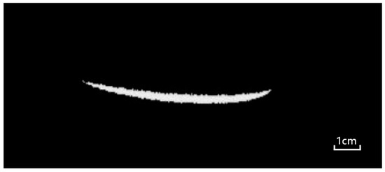
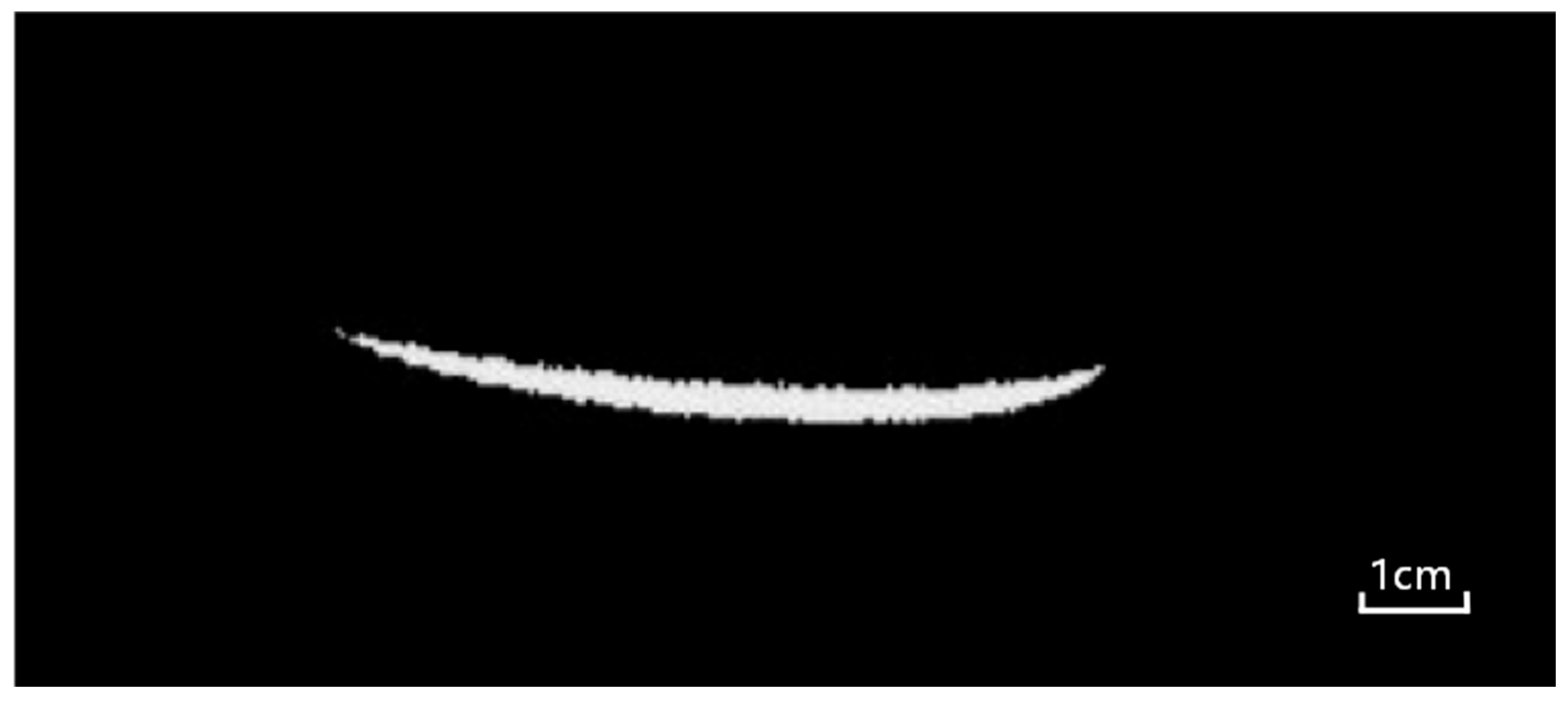
In addition, line laser images are highly susceptible to interference from external environmental and equipment factors during acquisition, such as ambient light noise, complex reflections on the surface of measured objects, and optical system distortion [13]. These interferences will further exacerbate the irregularity of the stripe grayscale distribution, posing challenges for subsequent centerline extraction work. The actual laser line fringe image is shown in Figure 1.
Figure 1.
Typical actual laser stripe image collected in an industrial inspection scenario, showing the inherent characteristics of non-uniform width and edge blur.
2.2. Basic Theories of Stripe Extraction Methods
Laser stripe center extraction is a core link in line laser 3D measurement, and its accuracy directly determines the effect of subsequent 3D reconstruction. Traditional stripe extraction methods and classic algorithms based on the Hessian matrix provide theoretical foundations for sub-pixel localization of stripe centers, while also having obvious limitations.
2.2.1. Classic Traditional Stripe Extraction Methods
Traditional laser stripe center extraction methods mainly rely on the grayscale or geometric features of stripes, with typical methods including the gray centroid method, threshold method, and skeleton extraction method.
- Gray Centroid Method
The core principle of this method is based on the assumption that the cross-sectional grayscale distribution of laser stripes conforms to a Gaussian distribution [14]. It calculates the weighted average of pixel coordinates using the grayscale values of pixels in the stripe region as weights, which is taken as the stripe center. Its calculation formula is as follows:
where denotes the coordinate of the stripe center, and represents the grayscale value of the pixel . This method features simple calculation and strong real-time performance. However, it is based on the fixed-width assumption, making it difficult to adapt to the non-uniform width variation in stripes in practical scenarios and prone to positioning deviation due to noise interference.
- Threshold Method
The threshold method segments the stripe region from the background by setting a grayscale threshold and extracts the geometric center of the stripe region as the stripe center. This method is easy to operate, but the selection of the threshold is highly subjective [15]. When the stripe edges are blurred or noise exists, over-segmentation or under-segmentation of the stripe region is likely to occur, resulting in reduced accuracy of center extraction.
- Skeleton Extraction Method
The skeleton extraction method shrinks the stripe region into a single-pixel-width skeleton line through morphological thinning operations [16], which is regarded as the stripe center. This method can retain the overall morphology of stripes, but the thinning process tends to lose stripe details and is sensitive to noise. In complex noise environments, it is prone to generating pseudo-skeletons, leading to centerline breakage.
2.2.2. Stripe Extraction Based on Hessian Matrix
The Hessian matrix is a classic mathematical tool for describing local grayscale changes in images. Its core principle is to construct a feature matrix by calculating the second-order partial derivatives of image pixels, and use the eigenvalues and eigenvectors of the matrix to characterize the direction, width, and center position of stripes, providing theoretical support for sub-pixel level center localization. For a pixel (x, y) in an image, its Hessian matrix is defined as:
where and are the second-order partial derivatives of the image grayscale respectively.
The two eigenvalues and of the Hessian matrix can reflect the grayscale variation characteristics of the local region: when the pixel is located at the stripe center, the grayscale variation along the tangent direction of the stripe is gentle, corresponding to the smaller eigenvalue ; the grayscale variation along the normal direction of the stripe is drastic, corresponding to the larger eigenvalue . Preliminary localization of the stripe center can be achieved by judging the magnitude relationship between the eigenvalues.
On this basis, sub-pixel level optimization of the stripe center can be realized by combining the Taylor expansion. However, the traditional Hessian matrix-based method lacks adaptive adjustment for stripe width, and the selection of Gaussian filtering scale depends on empirical values, making it difficult to adapt to stripes with non-uniform widths.
2.3. Limitations of Traditional Filtering and Anti-Interference Methods
The preprocessing of traditional laser stripe images primarily relies on various filtering algorithms for noise suppression and anti-interference, aiming to provide high-quality image input for subsequent stripe center extraction. However, these methods exhibit prominent limitations in practical applications, failing to balance noise suppression efficacy and stripe detail preservation.
Typical linear filtering methods, including Gaussian filtering and mean filtering, suppress noise via weighted averaging of adjacent image pixels [17]. As an isotropic smoothing process, linear filtering cannot distinguish between stripe edge details and noise signals. While mitigating noise, it inevitably smooths the sharp grayscale transitions at stripe edges, resulting in edge blurring and reduced contrast that hinder subsequent sub-pixel-level center extraction.
Nonlinear filtering methods represented by median filtering and bilateral filtering have partially improved edge detail retention. Median filtering replaces the original pixel value with the median of neighboring pixels, yielding a favorable suppression effect on impulse noise such as salt-and-pepper noise. Bilateral filtering achieves adaptive image smoothing by combining spatial distance and grayscale similarity weights. Nevertheless, these nonlinear methods still have shortcomings: median filtering shows limited efficacy in suppressing Gaussian noise with small grayscale differences from stripes; bilateral filtering involves high computational complexity, making it difficult to meet the real-time requirements of industrial online inspection. Moreover, both methods lack targeted processing strategies for laser stripe regions, leading to suboptimal anti-interference performance in complex noise environments.
In addition, the one-dimensional Finite Impulse Response (FIR) filter, commonly used in the preprocessing stage of stripe center extraction, mostly adopts a fixed 8-order design. Despite its linear phase characteristics and stability, it has significant limitations. On the one hand, its curvature adaptability is insufficient: the fixed order designed based on the ideal linear stripe assumption tends to cause over-smoothing in low-curvature regions, leading to edge detail loss, while in high-curvature regions, its smoothing capability is inadequate to suppress high-frequency noise effectively [18]. On the other hand, affected by the Gibbs Phenomenon, the filter generates oscillatory ripples when processing grayscale mutation regions such as stripe edges, forming pseudo-gray peaks that interfere with the accuracy of center positioning.
3. Laser Stripe Center Extraction Algorithm
3.1. Noise Interference Removal Preprocessing Method
To address the limitations of the traditional denoising methods described in Section 2.3, such as edge detail loss and difficulty in distinguishing between noise and stripes when processing line laser images, this paper proposes an improved U-Net++ [19] network based on the spatial attention mechanism, which is specially designed to eliminate noise around line laser stripes and provide high-fidelity image input for subsequent stripe center extraction. The noise distribution in the actual laser stripe image is shown in Figure 2, where the red box marks the typical ambient light noise and reflection noise near the stripe region, which is the core interference source that traditional filtering methods struggle to handle effectively. The core innovation of this method lies in embedding the spatial attention module into the dense skip connections of U-Net++, enabling the network to adaptively enhance the feature response of the line laser stripe region while suppressing background noise interference.
Figure 2.
Noise distribution in the actual laser stripe image. The region enclosed in the red box marks the typical ambient light noise and reflection noise near the stripe region, which is the core interference source for stripe center extraction.
3.1.1. Denoising Network Structure
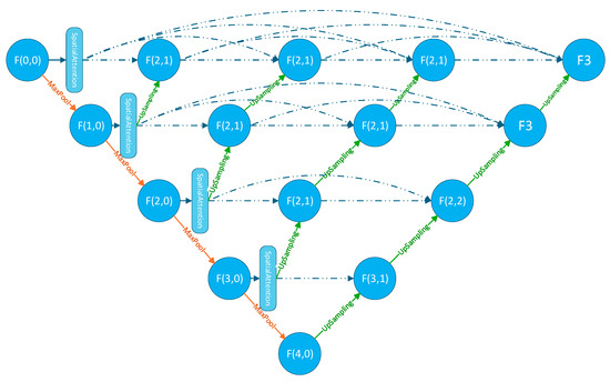
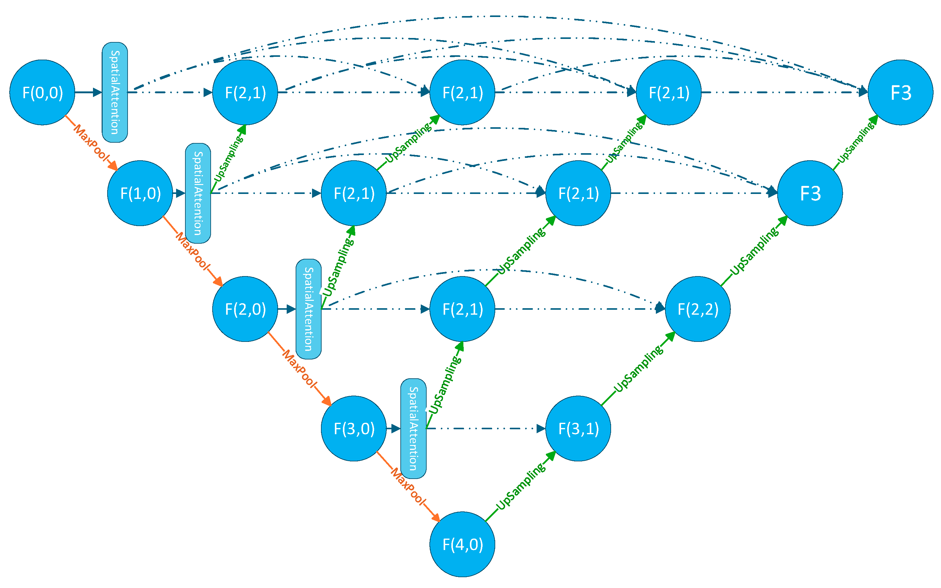
Figure 3 illustrates the overall architecture of the proposed spatial attention-based U-Net++ for linear stripe denoising. The network adopts a symmetric encoder–decoder design, consisting of 4 downsampling layers and 4 upsampling layers, with spatial attention modules incorporated at the skip connections.
Figure 3.
Overall architecture of the proposed spatial attention-based U-Net++ denoising network, consisting of an encoder path, a decoder path, and spatial attention modules embedded in the skip connections. The dashed lines in the figure denote the skip connections.
Noisy linear fringe images first enter the encoding path, where features are gradually extracted, and spatial resolution is reduced through a series of convolution and downsampling operations. After each encoding layer, the feature map is processed by a spatial attention module to generate a weighted feature map for subsequent skip connections. Following the bridge layer (the bottommost layer), the network enters the decoding path, where spatial resolution is gradually restored through upsampling and feature concatenation operations. After each upsampling step, the decoder-side features are concatenated with the corresponding encoder-side features (weighted by spatial attention) to achieve multi-scale feature fusion. Finally, the output layer generates a normalized grayscale denoised image through 1 × 1 convolution and a Sigmoid activation function, completing the regression mapping from the noisy image to the noise-free image. This architectural design retains the advantage of U-Net++ in multi-scale feature fusion, while precisely enhancing the feature response of linear fringe regions through the spatial attention mechanism, realizing targeted noise removal and dual preservation of fringe structures and grayscale details.
3.1.2. Distance Perception Denoising Mechanism
Based on the spatial distribution characteristics of noise near linear stripes, we propose a distance-aware denoising mechanism. The core idea of this mechanism is to dynamically adjust the denoising intensity according to the distance from each pixel to the nearest stripe, thereby effectively suppressing noise while protecting the stripe structure. For any pixel (x, y) in the laser stripe image, the distance weight W(d) is defined as a Gaussian kernel-based spatial weight function, whose value is determined by the Euclidean distance from the pixel to the nearest boundary of the laser stripe region. The explicit mathematical expression is:
where d denotes the distance from a pixel to the nearest stripe, and σ controls the suppression intensity. The closer a pixel is to the stripe, the lower the denoising intensity, to protect the stripe structure.
The calculation of distance d(x, y) is based on an initial coarse segmentation mask. First, the noisy image is subjected to thresholding using the Otsu method to obtain a binary mask M (Region of Interest, ROI) of the stripe region. Subsequently, the Euclidean Distance Transform algorithm is applied to compute a distance map d(x, y), where each pixel value represents the distance to the nearest stripe mask boundary. This method ensures robust distance calculation without relying on manual annotations.
Specifically, we define the region within 0.2w pixels from the stripe as the stripe core region (where w denotes the estimated stripe width obtained by the method described in Section 3.2). This region adopts the highest protection threshold to safeguard the stripe edge details. The region ranging from 0.2w to 0.5w pixels from the stripe is designated as the near-stripe region, where moderate denoising is performed on the pixels within this range. Finally, the far-stripe region refers to the area beyond 0.5w pixels from the stripe, where denoising is implemented with the maximum intensity. Details are shown in Table 1.
Table 1.
Distance-Aware Denoising.
In Equation (3), the parameter is not a fixed value but rather adaptively learned based on the image complexity and noise level:
To achieve precise supervision for regression-based denoising, a composite loss function is designed to balance pixel-level grayscale fidelity, structural similarity, and region-specific differentiated supervision. The formula is as follows:
Among them, denotes the distance-aware weight of the pixel ; represents the L1 loss term, which measures the pixel-level grayscale error between the denoised image and the noise-free ground truth image , ensuring grayscale fidelity while avoiding the problem of gradient explosion; is the structural similarity metric component. α and β are balance coefficients, set to 0.6 and 0.4, respectively, through experiments. The pseudocode of this algorithm is shown in Algorithm 1.
| Algorithm 1 Distance-Aware Adaptive Weight Generation Algorithm |
| Input: Noise image I |
| Output: Distance weight map W |
| M = threshold(I) // Generate binary mask, line area = 1, background = 0 |
| d = distance_transform(M) // Calculate distance from each pixel to nearest line |
| Compute connected component width from M or use the historical value |
| T1 = 0.2 * w, T2 = 0.5 * w // Replace fixed pixel thresholds |
| σ = σ0 · (1 + α · Complexity + β · NoiseLevel) // Equation (4) |
| W(d) = exp(−d2/(2σ2)) // Generate weight map |
| L_total = Σ_{i,j} W(d_{i,j}) · [α · |I(i,j) − K(i,j)| + β · (1 − SSIM_local(i,j))] // Equation (5) |
The core innovation of this loss function lies in the deep integration of regression-based supervision and spatially adaptive weights. It not only conforms to the inherent regression task nature of grayscale image denoising but also specifically addresses the contradiction between stripe detail preservation and background noise suppression in laser stripe denoising, providing high-fidelity image input for subsequent center extraction. The complete execution flow of the above algorithm is visually presented in Figure 4.
Figure 4.
Complete execution flowchart of the distance-aware adaptive weight generation algorithm, including the core steps of coarse segmentation, distance transform, stripe width estimation, weight map calculation, and weighted loss function construction.
3.2. Improved Hessian Matrix-Based Adaptive Weighted Average Width Stripe Center Extraction Algorithm
To address the problems of poor curvature adaptability and insufficient adaptive capacity for stripe width existing in the traditional line extraction methods described in Section 2.2, this paper proposes an adaptive weighted average width line extraction method based on an improved Hessian matrix. Innovatively, this method introduces a curvature-adaptive FIR filter, combines the direction template method with weighted screening to calculate the weighted average width of stripes, establishes an explicit mapping relationship between stripe width and Gaussian scale, and ultimately achieves high-precision sub-pixel level stripe center extraction. The overall workflow is as follows: first, curvature-adaptive FIR filtering is performed to optimize the grayscale distribution of stripes; second, the improved direction template method is adopted to calculate the local stripe width; next, the weighted average width is solved and mapped to the Gaussian scale; finally, the improved Hessian matrix is leveraged to realize sub-pixel center localization. The full execution flow of the algorithm is shown in Figure 5, which intuitively presents the logical connection between each sub-module of the center extraction algorithm.
Figure 5.
Overall execution flowchart of the proposed adaptive weighted average width stripe center extraction algorithm based on the improved Hessian matrix.
3.2.1. Curvature-Driven Order Selection Mechanism
To address the insufficient adaptability of traditional fixed-order FIR filters to stripe regions with different curvatures, this paper proposes a curvature-driven order selection mechanism. By dynamically matching the filter order with the local stripe morphology, it effectively suppresses noise while accurately preserving stripe edges and detail features, laying a high-quality preprocessing foundation for subsequent high-precision center extraction.
The core implementation process and key formulas of this mechanism are as follows: Direct curvature calculation on raw images is susceptible to noise interference; thus, Gaussian smoothing preprocessing is first applied to suppress high-frequency noise and stabilize grayscale gradients. The Gaussian kernel function is defined as:
where σ = 1.0 (verified through experiments to achieve the optimal balance between noise suppression and detail preservation). Based on differential geometry theory, an improved algorithm is adopted to calculate the local stripe curvature, which characterizes the degree of stripe bending:
where and denote the first-order derivatives, , , and denote the second-order derivatives, and is a small constant to avoid division by zero errors. To adapt to differences in curvature scales across different images, the calculated curvature values are first compared with a preset maximum threshold (0, 1) and normalized to the interval [0, 1]. Based on the normalized curvature κnorm, a nonlinear mapping function is designed to realize smooth adjustment of the filter order:
where denotes the normalized curvature, represents the base order, is the maximum allowable order, and is the adjustment parameter (with a default value of 3). The tanh function ensures that the order varies smoothly within the range [6, 12]. Leveraging the characteristics of the tanh function, this mapping adopts a lower-order filter in low-curvature regions to balance computational efficiency and basic smoothing needs, while using a higher-order filter in high-curvature regions to finely preserve stripe details, achieving intelligent matching between filter characteristics and stripe morphology.
3.2.2. Adaptive Weighted Average Width Extraction Method for Stripe Center Point Detection
The core of stripe center extraction based on the Hessian matrix is to determine the direction of the fastest grayscale decrease at each point through the matrix, and obtain sub-pixel coordinates via Taylor expansion. Its accuracy depends on the degree of conformity between the grayscale of the stripe cross-section and the ideal Gaussian distribution. However, in practical scenarios, laser stripes have pixel-level width and deviate from the standard Gaussian distribution due to interference from noise, light intensity, and other factors. Therefore, Gaussian filtering preprocessing is required first to enhance computational robustness. To address the problem of easy distortion of stripes on the surface of complex objects, four-directional (vertical, horizontal, 45°, and 135°) 17 × 3 all-1 templates are adopted. Valid stripe directions are determined through pixel-wise convolution and a weighted screening mechanism (the convolution response of a candidate direction must be greater than 1.1 times the convolution response of each of the other three directions to be determined as the effective stripe direction). For ideal linear stripes, the response ratio of the optimal direction to the sub-optimal direction is generally above 1.2, whereas this ratio drops to the range of 1.05 to 1.2 for non-uniform and curved stripes. This experimentally optimized 1.1 threshold achieves a well-balanced trade-off between direction discrimination capability and noise robustness, which not only mitigates erroneous direction identification induced by noise but also preserves the adaptability to curved stripes. Then, the local width is calculated by extending from the pseudo-center points along the cross-sectional direction. Combining the number of pseudo-center points corresponding to each local width, the global stripe width is solved using the weighted average method. Finally, this adaptive width is combined with the Hessian matrix to achieve high-precision stripe center localization.
In traditional methods, the Gaussian scale σ only provides a vague constraint (e.g., ) and lacks a quantitative correlation with the stripe width, resulting in insufficient adaptability of the Hessian matrix to stripes with non-uniform widths. The calculated adaptive weighted average width (denoted as ) is directly used as the input of the Gaussian scale, and an explicit linear mapping is established:
where k is the scale coefficient. According to the relationship between the full width at half maximum (FWHM) of the Gaussian function and , which satisfies:
To ensure that the Gaussian distribution fully covers the entire stripe width ( ≈ FWHM), it is derived that k ≈ 0.425. This coefficient was calibrated on the validation platform of the dataset used in this paper. It was found that when k = 0.4, the fitting error between the grayscale distribution of the stripe interface and the Gaussian distribution is the smallest. Thus, it is finally determined that:
The core advantage of this mapping relationship lies in the dynamic adjustment of the scale driven by adaptive width, which ensures consistent Gaussian fitting results for stripes in different regions, thereby enhancing the stability of feature extraction via the Hessian matrix.
4. Experiment
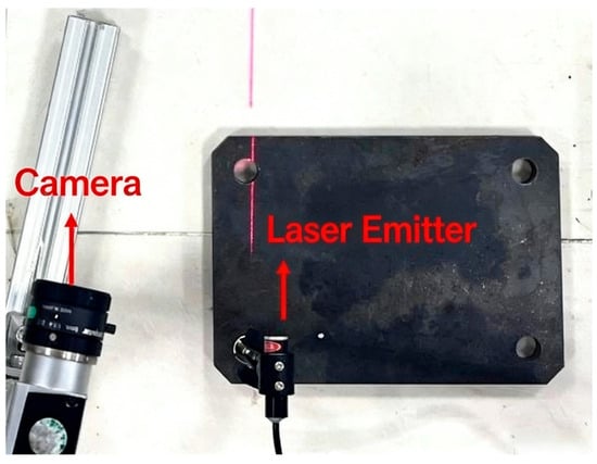
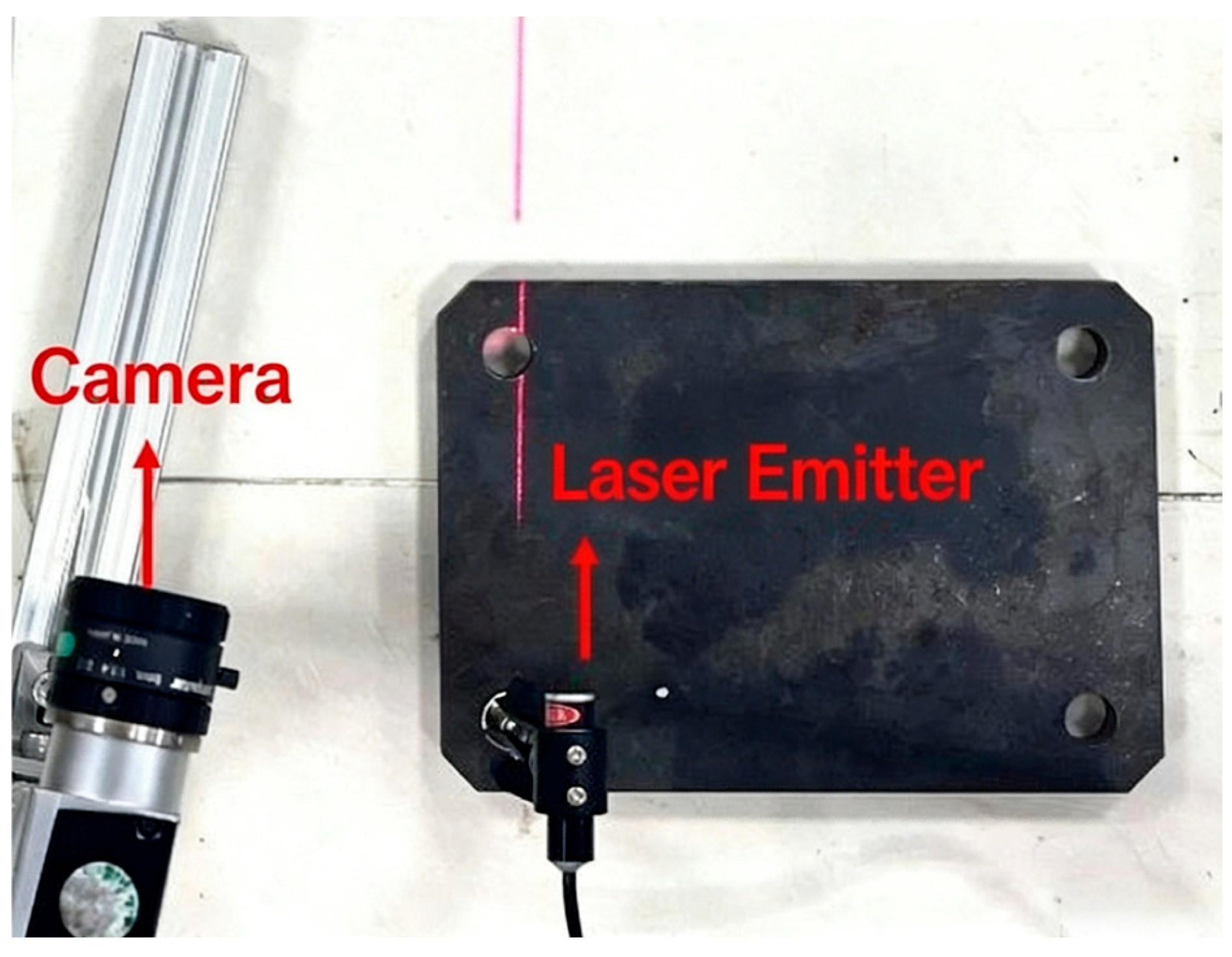
To verify the effectiveness of the improved Hessian matrix-based stripe center extraction algorithm with adaptive weighted average width, a set of line-structured light 3D reconstruction experimental setup was established. The experimental platform includes a 635 nm line laser transmitter (Model: MLL-III-635, Changchun New Industries Optoelectronics Tech. Co., Ltd., Changchun, China), a stepper motor, a GP150 12×9-10 (Lizhi, Dongguan, China) checkerboard calibration board, and a Basler acA1920-40gm camera (Basler AG, Ahrensburg, Germany). The detailed data of this camera is shown in Table 2. The constructed experimental setup of the line laser 3D reconstruction system is shown in Figure 6.
Table 2.
Core Imaging Specifications of the Basler acA1920-40gm Industrial Camera.
Figure 6.
Experimental setup of the line-structured light 3D reconstruction measurement system built in this paper, including a line laser transmitter and an industrial camera.
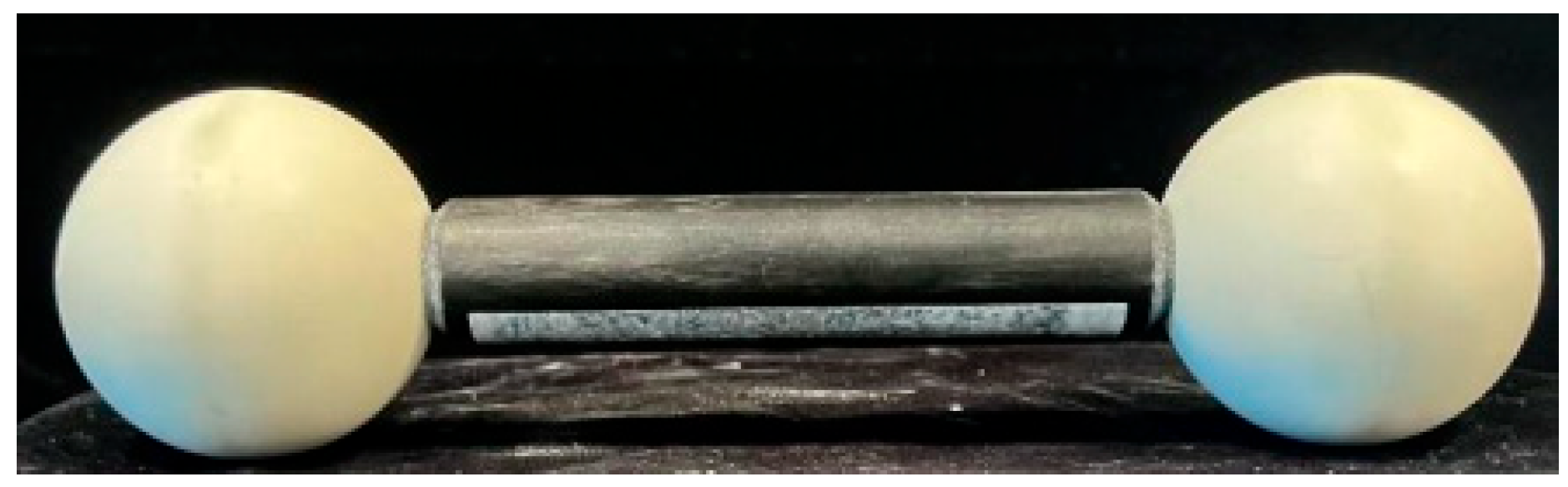
In this experiment, the workpiece under test is a matte ceramic dumbbell paddle with the model number DS-DCBD50.8L150, as shown in Figure 7.
Figure 7.
Physical diagram of the tested matte ceramic dumbbell paddle (model: DS-DCBD50.8L150), which is used as the standard workpiece for 3D reconstruction accuracy verification.
After capturing the data, the data is split into a training set, a test set, and a validation set, including 500 images for the training set, 300 for the test set, and 200 for the validation set. For data with insignificant noise, Gaussian noise is added for noise augmentation. The noise-added data is used to train the spatial attention U-Net++ network.
4.1. Denoising Network Experiment
The parameter settings for training the spatial attention U-Net++ network are as follows: the image size is 96 × 96. The experiment was conducted on an NVIDIA RTX4080S 16G graphics card with CUDA 11.8 and PyTorch 2.7.1 for 100 epochs, with a batch size of 8. The initial learning rate is 1 × 10⁻³, which decreases to 1 × 10⁻⁵ after 80 epochs. We used Peak Signal-to-Noise Ratio (PSNR), Structural Similarity Index Measure (SSIM), and Root Mean Square Error (RMSE) as indicators to evaluate the denoising performance of the network.
4.1.1. Evaluation Metrics
PSNR (Peak Signal-to-Noise Ratio) is calculated based on the mean square error of pixel grayscale values. A higher value indicates a smaller difference between the denoised image and the noise-free real image. To calculate PSNR, it is necessary to first compute the mean square error (MSE) between the denoised image and the noise-free real image:
where is the image height, is the image width, is the grayscale value of the pixel in the denoised image, and is the grayscale value of the corresponding pixel in the noise-free real image. After obtaining the MSE, substitute it into the PSNR formula:
SSIM (Structural Similarity Index Measure) evaluates image similarity from three dimensions: brightness, contrast, and structure. Its value ranges from [0, 1], and a value closer to 1 indicates more complete structure preservation. The calculation formula is as follows:
where and are the grayscale means of the denoised image and the noise-free image respectively; and are the grayscale variances of and respectively; is the grayscale covariance of and ; and are set to 0.01 and 0.03, respectively.
RMSE (Root Mean Square Error) is used to evaluate the pixel grayscale difference between the denoised image and the noise-free real image, reflecting the pixel-level fidelity of the denoising effect.
4.1.2. Experimental Results
To verify the advancement of our method, experiments were performed on the same dataset using standard U-Net [20], Swin U-Net [21], U-Net++, and our proposed method. The experimental results are the mean ± standard deviation of 5 independent experiments, as shown in Table 3:
Table 3.
Denoising Network. (Bold values indicate the optimal data).
As can be seen from the above table, our method achieves a PSNR of 35.26 dB, which is 2.81 dB higher than that of the standard U-Net and 1.54 dB higher than that of U-Net++. This significant improvement indicates that the proposed method has obvious advantages in terms of pixel-level fidelity, being able to more effectively suppress noise while preserving image details. It reaches 0.962 in SSIM, which is significantly higher than other comparative methods, demonstrating the method’s excellent performance in maintaining image structural information—especially in better preserving the edge structures and texture features of laser stripes. Meanwhile, the RMSE is reduced to 6.14, representing an error reduction of 29.6% compared with the standard U-Net. A lower RMSE value indicates a smaller difference between the denoised result and the real noise-free image. In terms of efficiency, although our method has slightly more parameters and a longer inference time than the original U-Net++, the magnitude of performance improvement far exceeds the increase in computational cost, reflecting excellent cost-effectiveness.
The experimental results for the balance coefficients α and β of the loss function are shown in the following table. As indicated by the data in Table 4, when α = 0.4 and β = 0.6, all evaluation metrics achieve the optimal performance.
Table 4.
Weight Parameters of The Loss Function. (Bold values indicate the optimal data).
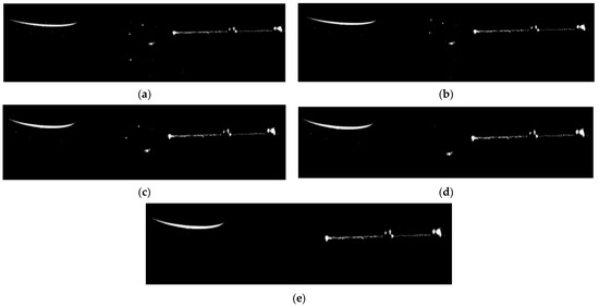
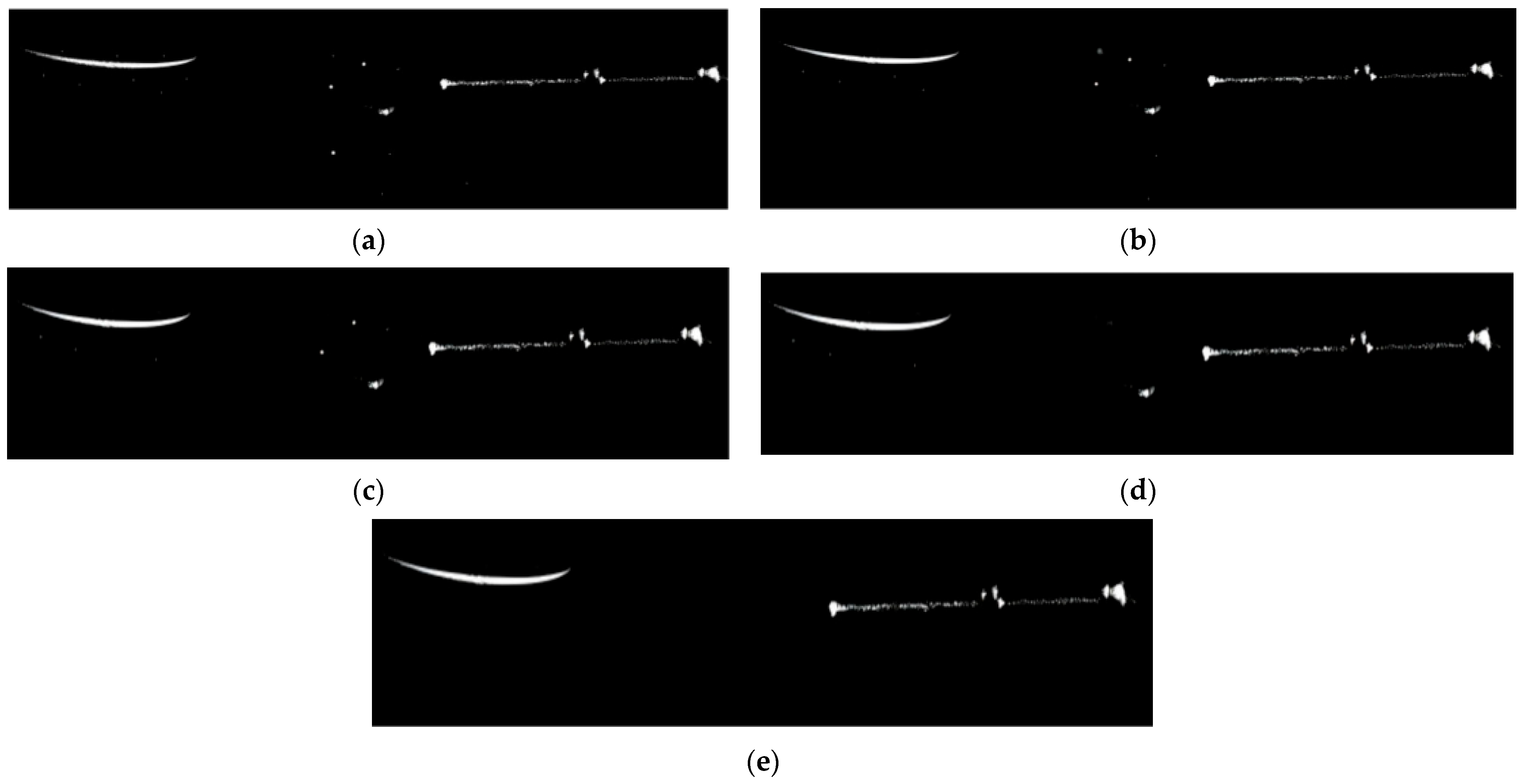
To more intuitively demonstrate the excellent performance of our method in image denoising, the denoising effects of the four networks on the dataset shown in Figure 8 are visually presented below:
Figure 8.
Visual comparison of denoising results of different networks. (a) Noisy original laser stripe image; (b) Denoising result of U-Net; (c) Denoising result of Swin U-Net; (d) Denoising result of U-Net++; (e) Denoising result of the proposed method in this paper.
From the visual comparison in Figure 8, it can be clearly observed that U-Net (Figure 8b) and Swin U-Net (Figure 8c) have obvious residual noise in the background region far from the stripe, and the edge of the laser stripe is blurred to varying degrees. This phenomenon is caused by the isotropic denoising strategy without targeted enhancement of the stripe region, which is consistent with the limitation of traditional U-Net series models analyzed in Section 1. U-Net++ (Figure 8d) achieves better background noise suppression, but there is still a slight edge detail loss in the high-curvature segment of the stripe, and the grayscale uniformity of the stripe core region is insufficient. In contrast, the proposed method (Figure 8e) completely eliminates ambient light noise and reflected noise in the background while maintaining the sharpness of the stripe edge, and the grayscale distribution of the stripe core region is highly consistent with the original noise-free image. Especially in the curved segment of the stripe, the proposed method avoids edge-smoothing distortion caused by over-denoising, and fully retains the morphological characteristics of the laser stripe.
Table 5 presents the comparison results of comprehensive performance metrics of the four variant models on the test set, including Peak Signal-to-Noise Ratio (PSNR), Structural Similarity Index Measure (SSIM), and Root Mean Square Error (RMSE).
Table 5.
Ablation Experiments.
Based on the ablation experiment results shown in Table 5, we can conduct a systematic analysis of the two core innovative modules proposed in this paper—the Distance-Aware Mechanism and the Spatial Attention Mechanism. The independent contribution of the Distance-Aware Mechanism is reflected in the data of the second row. After independently introducing the Distance-Aware Mechanism, the PSNR increases to 34.15 ± 1.02 dB with an increase of 0.43 dB; the SSIM rises to 0.951 ± 0.013; and the RMSE is reduced to 6.89 ± 0.79. This improvement confirms the effectiveness of the Distance-Aware Mechanism, which dynamically adjusts the denoising intensity according to the distance between pixels and stripes, effectively suppressing noise while protecting edge details.
The independent effect of the Spatial Attention Mechanism is demonstrated by the data in the third row. When only the Spatial Attention is enabled, the PSNR reaches 34.58 ± 0.98 dB, an increase of 0.86 dB compared with the baseline; the SSIM increases to 0.956 ± 0.012; and the RMSE decreases to 6.47 ± 0.76. This significant improvement indicates that the Spatial Attention Mechanism can guide the network to focus on stripe regions and enhance the expressive ability of key features.
When both the Distance-Aware and Spatial Attention mechanisms are enabled, the model achieves optimal performance: the PSNR reaches 35.26 ± 0.95 dB, the SSIM is 0.962 ± 0.012, and the RMSE is as low as 6.14 ± 0.74. It is worth noting that the magnitude of performance improvement of the complete model (a 1.54 dB increase in PSNR) is greater than the sum of the independent contributions of the two modules (0.43 + 0.86 = 1.29 dB), indicating a synergistic enhancement effect between the two innovative modules. The Distance-Aware Mechanism optimizes the denoising strategy from the pixel-level dimension, while the Spatial Attention Mechanism enhances the response of key regions from the feature map level. Together, they jointly improve the denoising capability of the network from different scales. PSNR, SSIM, and RMSE of the denoising network are only used as auxiliary evaluation metrics, and their performance is ultimately verified by the subsequent measurement of closed-loop metrics of center extraction.
4.2. Stripe Center Extraction Algorithm
The method proposed in this paper utilizes the characteristics of the direction template method to determine the stripe edge direction of the captured stripe images. It adopts templates in four different directions (horizontal, 45°, vertical, and 135°) to convolve the stripe images.
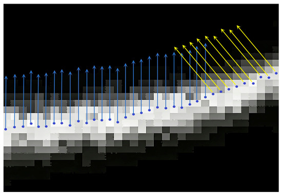
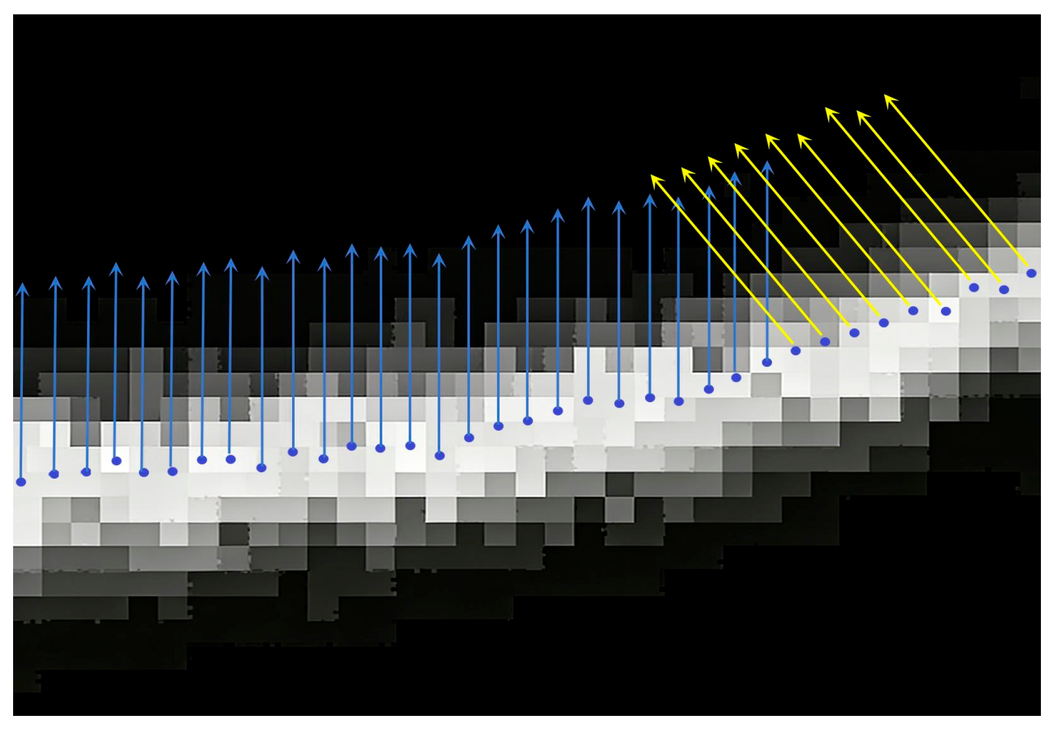
By comparing the convolution values of the four direction templates in the same pixel grid, the direction template with a response value significantly greater than those of the other three directions is regarded as the most probable stripe direction of the stripe pseudo-center point. Starting from the stripe pseudo-center points obtained in Section 3.2.2, the width of the stripe’s foreground pixels at each pseudo-center point is acquired along the direction perpendicular to the stripe direction—i.e., the cross-sectional direction of the stripe. The schematic diagram of the extension direction when solving the corresponding stripe width for the stripe pseudo-center points is shown in Figure 9.
Figure 9.
Schematic diagram of the width-solving direction for stripe pseudo-center points. The width of the stripe is calculated along the normal direction of the stripe (perpendicular to the tangent direction of the stripe), starting from the pseudo-center point. The arrow in the figure indicates the cross-sectional direction of the stripe. The blue points represent the center points.
In the experiment, the left ball of the matte ceramic ball dumbbell racket was uniformly used to reconstruct point clouds. The difference between the fitted sphere radius of the standard ball reconstructed by different algorithms and its true radius value (25.40 mm) was compared to verify the effectiveness of the proposed algorithm in improving the accuracy of center point extraction. Five mainstream traditional laser stripe center extraction algorithms were compared, namely the optimized Zhang-Suen thinning method, the gray centroid method, the Steger algorithm, the Hessian-based adaptive weighted width algorithm proposed by Wang et al. [10] in 2024, and the optimized algorithm proposed in this paper. The comparative data of the 3D reconstruction results of the standard ball using different stripe center point extraction algorithms under different exposure conditions are presented in Table 6, Table 7, Table 8 and Table 9.
Table 6.
Measurement Errors of Standard Sphere Radius under 200 μs Exposure. (Bold values indicate the optimal data).
Table 7.
Measurement Errors of Standard Sphere Radius under 500 μs Exposure. (Bold values indicate the optimal data).
Table 8.
Measurement Errors of Standard Sphere Radius under 1000 μs Exposure. (Bold values indicate the optimal data).
Table 9.
Measurement Errors of Standard Sphere Radius under 1500 μs Exposure. (Bold values indicate the optimal data).
There are two categories of evaluation metrics in this experiment: error metrics and stability metrics. The error metrics include centerline pixel error, absolute radius error, and RMSE. The centerline pixel error refers to the absolute radius error, which is the absolute value of the difference between the measured radius and the true radius of the standard ball (25.4 mm); the RMSE refers to the root mean square error of the distance between the reconstructed point cloud and the surface of the real sphere. The stability metrics include centerline breakage rate and redundant point rate. The centerline breakage rate is the ratio of the number of breakpoints to the total length of the centerline (in pixels), where a breakpoint is defined as a point with an interval of ≥3 pixels in the continuous centerline; the redundant point rate is the ratio of the number of isolated points to the total number of extracted points, where an isolated point is defined as a discrete point that is ≥2 pixels away from the main body of the centerline.
In this experiment, the effectiveness of the proposed algorithm was quantitatively evaluated by comparing the radius errors of standard spheres reconstructed using different laser stripe center extraction algorithms. Analyzing the data in Table 7, Table 8 and Table 9, the following conclusions can be drawn: The proposed algorithm exhibits significant advantages in extraction accuracy compared with traditional algorithms: under three different exposure durations (500 μs, 1000 μs, 1500 μs), the absolute radius error of the standard sphere reconstructed by the proposed algorithm is slightly higher than that of the algorithm proposed by Wang et al. in 2024 only under the 500 μs exposure time, while demonstrating excellent extraction accuracy under other conditions. In particular, under the 1000 μs and 1500 μs exposure conditions, its absolute errors (0.0268 mm and 0.0281 mm, respectively) are significantly lower than those of other comparative algorithms. This indicates that the 3D model reconstructed using the center points extracted by this algorithm has the closest size to the true value, verifying its effectiveness in improving the accuracy of center point extraction.
The proposed algorithm possesses good robustness compared with traditional algorithms: as the exposure time changes, the measurement errors of other algorithms fluctuate to a certain extent. For example, the gray centroid method has a large error (0.1974 mm) at 500 μs, performs moderately (0.0931 mm) at 1000 μs, but the error increases again (0.1353 mm) at 1500 μs. In contrast, the error of the proposed algorithm changes relatively stably with the exposure time, and achieves optimal performance under the optimal exposure conditions (such as 1000 μs and 1500 μs), demonstrating good robustness and adaptability. Meanwhile, the proposed algorithm achieves the minimum absolute radius error while maintaining a low RMSE (i.e., good point cloud smoothness), realizing the optimal balance between point cloud quality and dimensional accuracy. This indicates that its optimization effectively reduces system deviations.
In summary, the quantitative data fully prove that compared with mainstream traditional algorithms, the proposed optimized algorithm can extract laser stripe centers more accurately under different exposure conditions, thereby obtaining 3D reconstruction results with higher dimensional accuracy and better quality.
As core indicators for measuring the stability of stripe center extraction, the breakage rate and redundant point rate directly reflect the algorithm’s ability to maintain stripe continuity and suppress discrete noise points—a lower breakage rate indicates better integrity of the centerline, and a lower redundant point rate means higher purity of the extracted center points. In all exposure scenarios, the breakage rate and redundant point rate of the proposed algorithm are the lowest, showing a significant gap with traditional algorithms. As the exposure time increases from 500 μs to 1500 μs, the breakage rate and redundant point rate of all algorithms show a downward trend, because the reduction in noise improves stripe continuity and reduces discrete noise points. However, the proposed method has a larger decline range and better final values, reflecting stronger environmental adaptability.
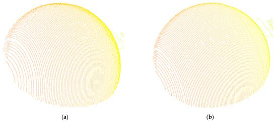
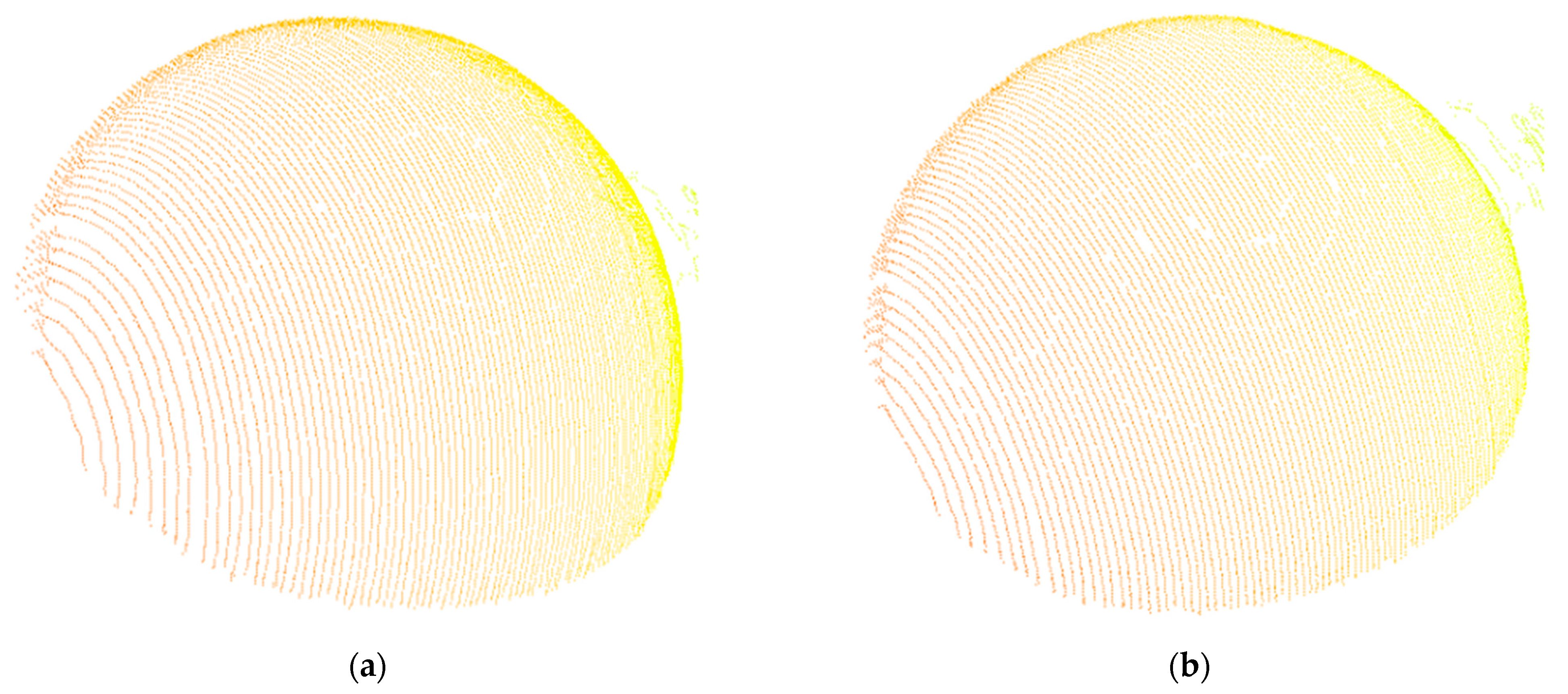
Figure 10 presents the 3D reconstruction results of the standard sphere obtained by the algorithm proposed by Wang et al. and the proposed method in this paper under the 1500 μs exposure condition. It can be seen from the figure that, compared with the algorithm proposed by Wang et al., the reconstructed standard sphere using the proposed method has a smoother surface and fewer breakpoints.
Figure 10.
Point cloud reconstruction results of the standard sphere under 1500 μs exposure. (a) Reconstruction result of the proposed algorithm in this paper; (b) Reconstruction result of the algorithm proposed by Wang et al. [10].
There are two core differences between the proposed algorithm and Wang et al. (Hessian-based adaptive weighted width algorithm): first, the design of the denoising module. This paper introduces the spatial attention U-Net++, combined with a distance-aware mechanism to achieve targeted denoising of stripe regions, solving the problem of small grayscale differences between noise and stripes under low exposure. In contrast, Wang et al. did not design a dedicated denoising module and relied on traditional Gaussian filtering, which has limited ability to suppress complex noise.
Second, the optimization of the extraction module. This paper proposes a curvature-adaptive FIR filter that dynamically adjusts the filter order (adaptive variation between 6 and 12 orders) to adapt to high-curvature stripes. However, Wang et al. adopted a fixed window weighting strategy, which is insufficient in preserving details in regions with sudden curvature changes.
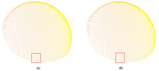
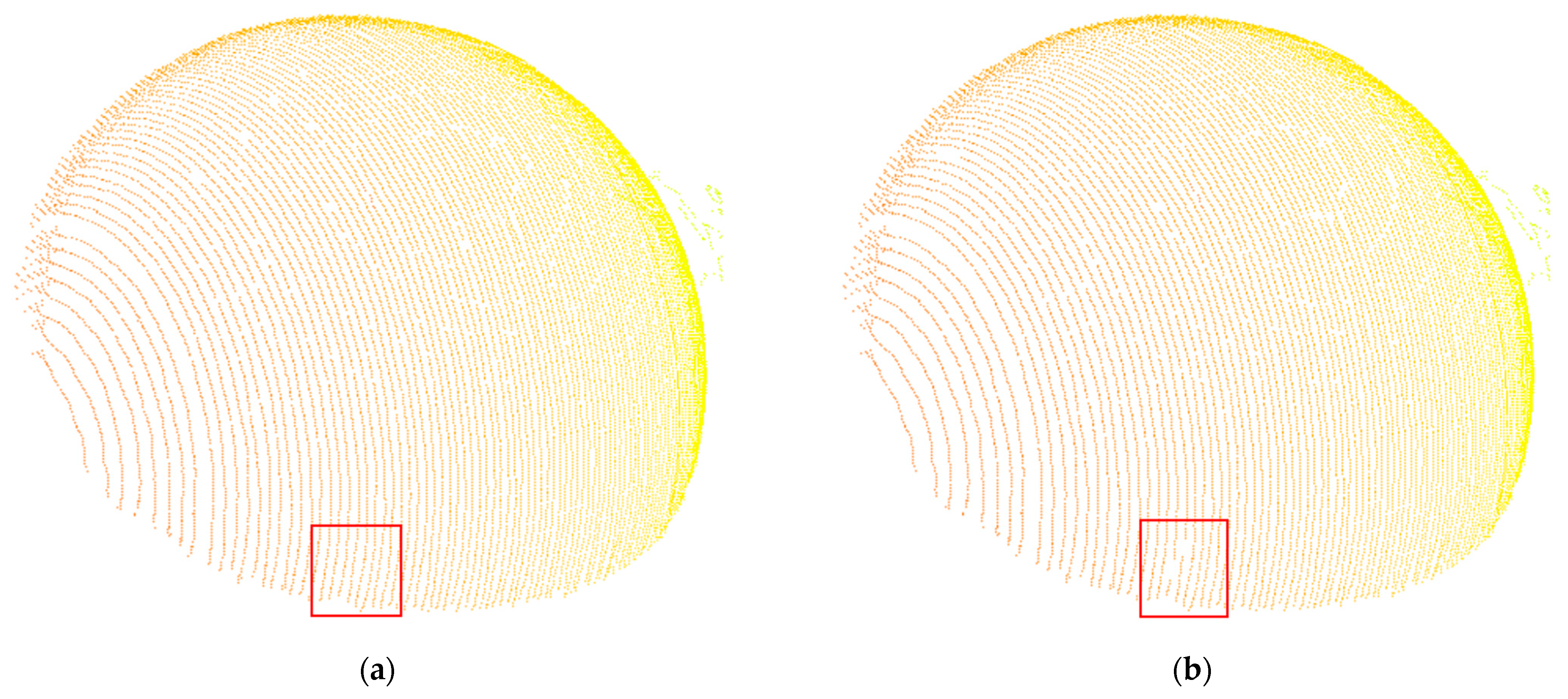
As can be observed from Figure 11, the experimental results show that under 500 μs exposure, the grayscale difference between environmental light noise and stripes is small (SNR ≈ 18 dB), resulting in a slightly higher absolute radius error (0.174 mm) of the proposed method than that of Wang et al. 2024 [10] (0.143 mm). The main reason is that the grayscale gradient of stripe edges is weak under low exposure. To avoid blurring edge details, the distance-aware denoising mechanism in this paper performs conservative suppression on some noise close to the stripe grayscale, leading to a small amount of residual noise. Nevertheless, the breakage rate (0.028%) and redundant point rate (0.025%) of the proposed method are still superior to all comparative methods. With the increase in exposure time (1000 μs, 1500 μs), the collaborative advantages of noise suppression and curvature adaptation become prominent, and the absolute radius error decreases to 0.0268 mm and 0.0281 mm, making it the optimal solution. This phenomenon verifies the complexity of the denoising-extraction collaborative optimization under low-exposure scenarios, and also indicates that the proposed algorithm has higher reliability in medium and high exposure conditions (commonly used industrial scenarios).
Figure 11.
Point cloud reconstruction results of the standard sphere under 500 μs exposure. (a) Reconstruction result of the algorithm proposed by Wang et al. [10]; (b) Reconstruction result of the proposed algorithm in this paper. The red box shows the point cloud comparison of the edge regions.
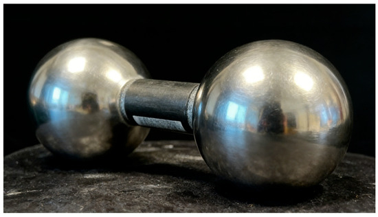
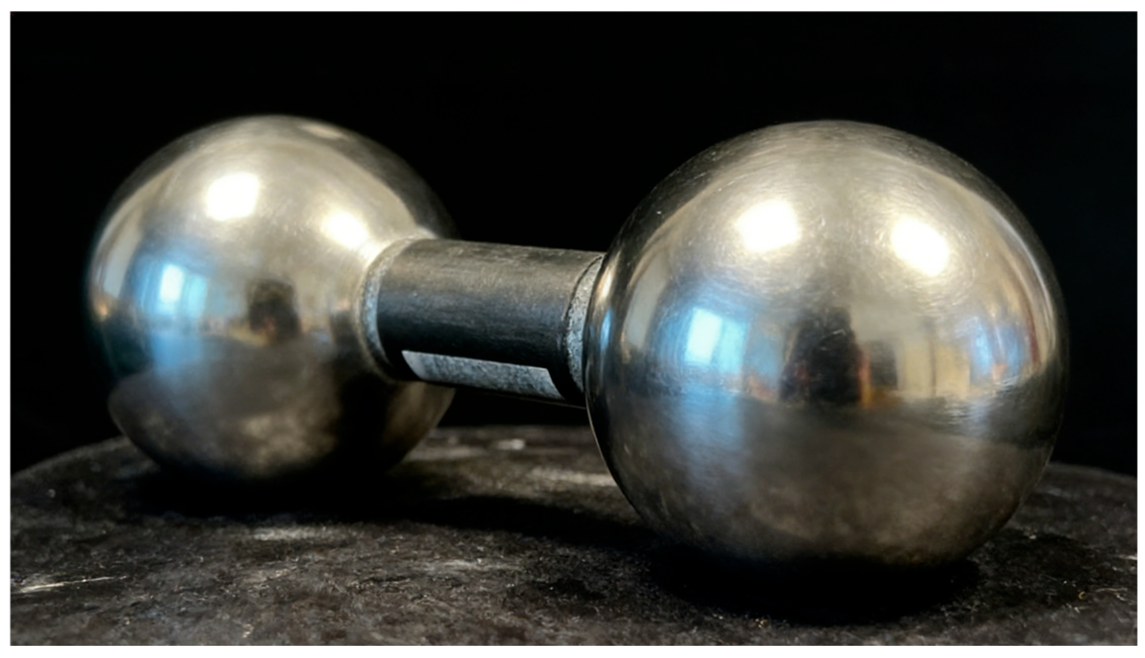
To verify the performance of the proposed method on highly reflective surfaces, we selected a metal dumbbell with a diameter of 5 cm for the experiment, and the experimental results are shown in Table 10. Quantitative results verify that even on highly reflective metal surfaces with severe specular reflection interference, the proposed method still achieves significantly higher extraction accuracy and better stability, consistently outperforming all the other comparative algorithms evaluated in this work.
Table 10.
Measurement Errors of Standard Sphere Radius on Highly Reflective Metal Surfaces. (Bold values indicate the optimal data).
The metal dumbbell workpiece shown in Figure 12 has a highly reflective smooth surface, which will cause severe specular reflection, stripe width non-uniformity and strong background noise during laser imaging. This is a common pain point in industrial metal parts inspection, and it is also a key scenario to verify the anti-interference performance of the proposed algorithm.
Figure 12.
Metal dumbbell workpiece with a highly reflective surface used in the anti-interference performance verification experiment.
Experiments on the Gaussian smoothing scale σ and scale coefficient k are presented in Table 11 and Table 12.
Table 11.
Performance Comparison of Different Gaussian Smoothing Scales σ (1500 μs). (Bold values indicate the optimal data).
Table 12.
Scale Coefficient k (1500 μs). (Bold values indicate the optimal data).
5. Discussion
This study aims to address the long-standing bottleneck in laser stripe center extraction: the inability of traditional algorithms to balance denoising performance and positioning accuracy, especially when processing stripes with complex noise and non-uniform width. By integrating deep learning-based denoising and improved Hessian matrix-guided center extraction, we proposed a collaborative optimization framework that achieves significant performance improvements in both denoising fidelity and 3D measurement accuracy. In this section, we interpret the core findings of our experiments, compare our work with state-of-the-art published studies, explain the underlying mechanisms of the observed experimental phenomena, clarify the limitations of the current work, and elaborate on the theoretical and engineering implications of this study.
5.1. Mechanistic Interpretation of Key Experimental Phenomena
Our experimental results show that the performance of the proposed algorithm shows regular changes under different exposure conditions, and we further interpret the underlying mechanism behind this phenomenon. Under medium and high exposure conditions (1000 μs and 1500 μs), the algorithm achieves the optimal comprehensive performance, with the lowest absolute radius error, centerline breakage rate, and redundant point rate. This is because under these conditions, the stripe has a high signal-to-noise ratio (SNR), the distance-aware denoising mechanism can accurately distinguish stripe edges from background noise, and the curvature-adaptive extraction module can fully exert its sub-pixel positioning advantage by relying on the complete gradient information of the stripe edges.
In contrast, under low exposure conditions (200 μs and 500 μs), the absolute radius error of the algorithm increases slightly, but it still maintains the lowest breakage rate and redundant point rate among all comparative algorithms. The underlying reason is that under low exposure, the gray difference between the stripe and ambient light noise is extremely small (SNR ≈ 18 dB). To avoid blurring the edge details that are critical for center positioning, our distance-aware denoising mechanism adopts conservative suppression for noise close to the stripe gray level, resulting in a small amount of residual noise. This is essentially a trade-off we actively choose: unlike existing low-exposure optimization algorithms that often over-smooth stripe edges to reduce noise, our algorithm prioritizes the integrity of the stripe edge structure, which is the core prerequisite for continuous and high-precision centerline extraction. This also explains why our algorithm still maintains the best centerline continuity under low exposure, which is more important for practical industrial 3D reconstruction than single-point pixel error.
In addition, the algorithm shows significant advantages in the measurement of highly reflective metal surfaces, which is a common pain point in industrial inspection. The specular reflection on the metal surface will cause severe non-uniformity of stripe width and strong background noise, leading to centerline offset and breakage in traditional algorithms. Our collaborative optimization framework solves this problem from two dimensions: the spatial attention denoising module suppresses strong reflection noise while focusing on the stripe region, and the adaptive weighted average width extraction module adapts to the sudden change in stripe width caused by reflection, thus achieving an absolute radius error of 0.144 mm on highly reflective surfaces, which is 39.7% lower than the algorithm of Wang et al. [10], verifying the strong robustness of the algorithm in complex industrial scenarios.
5.2. Limitations of the Current Study
To maintain the academic rigor of the study, we objectively clarify the limitations of the current work, which also provides a clear direction for subsequent optimization. First, the performance of the algorithm in extremely low-exposure environments (exposure time < 200 μs) still has room for optimization. When the exposure time is lower than 200 μs, the SNR of the stripe image drops sharply, and the gray gradient of the stripe edge is extremely weak, resulting in a significant increase in the absolute radius error of the algorithm, which cannot meet the needs of ultra-short exposure high-speed measurement scenarios.
Second, the lightweight of the denoising network still needs to be improved. Although the current inference time of 19.8 ms can meet the needs of most industrial offline and semi-real-time inspection scenarios, for high-speed real-time detection scenarios on edge devices (frame rate > 100 fps), the parameter size and inference speed of the model still need to be further optimized. Third, the current experimental verification is mainly based on standard spheres and regular workpieces in the laboratory, and the adaptability of the algorithm to extremely complex free-form surfaces (such as large curvature, strong, reflective, and irregular surfaces) still needs more engineering verification in actual industrial scenarios.
6. Conclusions
This study addresses the core challenge in 3D measurement: traditional laser stripe center extraction algorithms cannot balance noise suppression and positioning accuracy for stripes with complex noise and non-uniform widths. A denoising-extraction collaborative optimization algorithm, integrating deep learning with enhanced traditional image processing, is proposed to tackle this bottleneck.
For denoising, a U-Net++ network with spatial attention and distance-aware mechanisms is developed. The spatial attention module focuses on stripe regions adaptively, while the distance-aware strategy adjusts denoising intensity by pixel-stripe distance, achieving precise noise reduction without blurring edges. Experimental results show it attains a 35.26 dB PSNR, 0.962 SSIM, and 6.14 RMSE, outperforming U-Net and U-Net++ by 2.81 dB and 1.54 dB in PSNR, respectively.
In center extraction, an improved Hessian matrix-based algorithm with adaptive weighted average width is designed. A curvature-adaptive FIR filter (order 6–12) balances noise suppression and detail retention. Combined with the directional template method, it calculates stripe width and establishes an explicit mapping σ = 0.4 ω, enhancing adaptability to non-uniform widths.
Tests on a self-built platform demonstrate exceptional performance: under 1000 μs and 1500 μs exposure conditions (the most widely used in industrial high-precision measurement), the algorithm achieves absolute radius errors of 0.0268 mm and 0.0281 mm respectively—31.3% and 33.1% lower than the state-of-the-art Wang et al. 2024 [10] algorithm, and more than 70% lower than traditional methods such as the Steger algorithm. It also maintains the lowest centerline breakage rate (0.12%) and redundant point rate (0.10%) at 1500 μs, and meets real-time requirements with a 19.8 ms inference time. Even under 500 μs low exposure, it retains excellent stability with the lowest redundant point rate, verifying its strong adaptability to diverse industrial scenarios.
Future work will optimize performance in extremely low-exposure environments and explore lightweight models for edge computing deployment, advancing 3D measurement technologies.
Author Contributions
Conceptualization: G.L. and K.T.; Methodology: G.L. and W.M.; Software: G.L. and B.W.; Validation: G.L., K.T. and B.W.; Writing—original draft preparation: G.L.; Writing—review and editing: W.M. and S.Q.; Supervision: W.M. All authors have read and agreed to the published version of the manuscript.
Funding
This work was supported by the National Key R&D Program of China (grant number: 2024YFB4303202).
Informed Consent Statement
This article does not involve studies with human participants or animals.
Data Availability Statement
The data supporting the findings of this study are available from the corresponding author upon reasonable request.
Conflicts of Interest
Authors Gaokun Liu and Shaofeng Qiu were employed by the company China Railway Siyuan Survey and Design Group Co., Ltd. The remaining authors declare that the research was conducted in the absence of any commercial or financial relationships that could be construed as a potential conflict of interest.
References
- Lu, X.; Gu, D.; Wang, Y.; Qu, Y.; Qin, C.; Huang, F. Feature extraction of welding seam image based on laser vision. IEEE Sens. J. 2018, 18, 4715–4724. [Google Scholar] [CrossRef] [Scilit]
- Liu, C.; Duan, F.; Fu, X.; Li, J.; Li, T.; Han, P.; Ai, S. A novel method to correct the bias of curvilinear light stripe center. Opt. Lasers Eng. 2022, 155, 107058. [Google Scholar] [CrossRef] [Scilit]
- Steger, C. An unbiased detector of curvilinear structures. IEEE Trans. Pattern Anal. Mach. Intell. 1998, 20, 113–125. [Google Scholar] [CrossRef] [Scilit]
- Zhang, K.; Zuo, W.; Chen, Y.; Meng, D.; Zhang, L. Beyond a gaussian denoiser: Residual learning of deep CNN for image denoising. IEEE Trans. Image Process. 2017, 26, 3142–3155. [Google Scholar] [CrossRef] [Scilit] [PubMed]
- Peng, Y.; Chen, D.Z.; Sonka, M. U-Net V2: Rethinking the skip connections of U-Net for medical image segmentation. In Proceedings of the 2025 IEEE 22nd International Symposium on Biomedical Imaging (ISBI), Houston, TX, USA, 14–17 April 2025. [Google Scholar]
- Crespo, J.M.; Moreno, V.; Rabuñal, J.R.; Pazos, A.; Carbia, M.C. Fringe Pattern Denoising using U-Net based neural network. EPJ Web Conf. 2020, 238, 06009. [Google Scholar] [CrossRef] [Scilit]
- Zhang, H.; Lian, Q.; Zhao, J.; Wang, Y.; Yang, Y.; Feng, S. RatUNet: Residual U-Net based on attention mechanism for image denoising. PeerJ Comput. Sci. 2022, 8, e970. [Google Scholar] [CrossRef] [Scilit] [PubMed]
- Zou, W.; Wei, Z. A fast adaptive subpixel extraction method for light stripe center. In International Conference on Image and Graphics; Springer International Publishing: Cham, Switzerland, 2019. [Google Scholar]
- Li, Z.; Ma, L.; Long, X.; Chen, Y.; Deng, H.; Yan, F.; Gu, Q. Hardware-oriented algorithm for high-speed laser centerline extraction based on Hessian matrix. IEEE Trans. Instrum. Meas. 2021, 70, 5010514. [Google Scholar] [CrossRef] [Scilit]
- Li, J.; Wang, L.; Wan, Y.; Yang, K.; Luo, L. An adaptive weighted width extraction method based on the Hessian matrix for high-precision detection of laser stripe centers in low-exposure. Opt. Lasers Eng. 2024, 181, 108436. [Google Scholar] [CrossRef] [Scilit]
- Chu, Y.; Madhuranthakam, Y.; Miles, Z.; Karim, F.; Poudel, A.; Deng, Y.; Han, M.; Chakrapani, S.K. Laser generated surface acoustic wave using diffractive optical elements. Opt. Lasers Eng. 2025, 195, 109325. [Google Scholar] [CrossRef] [Scilit]
- Huang, Y.; Kang, W.; Lu, Z. Improved structured light centerline extraction algorithm based on unilateral tracing. Photonics 2024, 11, 723. [Google Scholar] [CrossRef] [Scilit]
- Liu, G.; Qiu, S.; Ma, W. Laser stripe Hessian sub-pixel localization based on pseudo-center points and dynamic width constraints. In Sixteenth International Conference on Information Optics and Photonics (CIOP 2025); SPIE: Bellingham, WA, USA, 2025; Volume 13990. [Google Scholar]
- Zeng, Q.; Huang, Z.; Yu, X.; He, W.; Liu, X.; Peng, X.; Tang, Q. Temporal line-shifting structured light for robust high-precision 3D reconstruction. Opt. Express 2025, 33, 27255–27269. [Google Scholar] [CrossRef] [Scilit] [PubMed]
- Zhao, X.; Wu, G.; Liu, G.; Song, Z.; Feng, F.; Liu, B.; Wu, Y. Robust centerline extraction method of laser stripe based on an underwater line scanning lidar. Opt. Lasers Eng. 2025, 188, 108898. [Google Scholar] [CrossRef] [Scilit]
- Miao, L.; Yin, J.; Zhang, D.; Gao, D.; Liang, H. Defect measurement technology based on skeleton extraction. In Fifth International Conference on Advanced Algorithms and Signal Image Processing (AASIP 2025); SPIE: Bellingham, WA, USA, 2025; Volume 13967. [Google Scholar]
- Duan, J.; He, Y.; Wu, X.; Zhang, H.; Wu, W. Anti-Interference deep visual identification method for fault localization of transformer using a winding model. Sensors 2019, 19, 4153. [Google Scholar] [CrossRef] [Scilit] [PubMed]
- Wu, Y.; Wang, Y.; Jiang, L.; Yu, J. Dispersion Compensation Scheme with a Simple Structure in Ultra-High-Speed Optical Fiber Transmission Systems. Photonics 2025, 13, 39. [Google Scholar] [CrossRef] [Scilit]
- Zhou, Z.; Siddiquee, M.M.R.; Tajbakhsh, N.; Liang, J. Unet++: A nested u-net architecture for medical image segmentation. In International Workshop on Deep Learning in Medical Image Analysis; Springer International Publishing: Cham, Switzerland, 2018. [Google Scholar]
- Ronneberger, O.; Fischer, P.; Brox, T. U-net: Convolutional networks for biomedical image segmentation. In International Conference on Medical Image Computing and Computer-Assisted Intervention; Springer International Publishing: Cham, Switzerland, 2015. [Google Scholar]
- Cao, H.; Wang, Y.; Chen, J.; Jiang, D.; Zhang, X.; Tian, Q.; Wang, M. Swin-unet: Unet-like pure transformer for medical image segmentation. In European Conference on Computer Vision; Springer Nature: Cham, Switzerland, 2022. [Google Scholar]







Disclaimer/Publisher’s Note: The statements, opinions and data contained in all publications are solely those of the individual author(s) and contributor(s) and not of MDPI and/or the editor(s). MDPI and/or the editor(s) disclaim responsibility for any injury to people or property resulting from any ideas, methods, instructions or products referred to in the content. |
© 2026 by the authors. Licensee MDPI, Basel, Switzerland. This article is an open access article distributed under the terms and conditions of the Creative Commons Attribution (CC BY) license.