Approximating Incoherent Monochromatic Light Sources in FDTD Simulations

Abstract

Light-emitting diodes (LEDs) are becoming increasingly important across various sectors of the lighting industry and are being used more frequently. In the field of symbolic projection, research is increasingly focusing on implementing light modulation using energy-efficient, incoherent LEDs rather than lasers. Since light modulation in micro- and nano-optics is typically achieved through phase modulation, Finite-Difference Time-Domain (FDTD) simulations are employed for analysis. The objective of this article is to investigate different approaches for approximating incoherent monochromatic light sources within FDTD simulations. To this end, two approaches based on dipole sources are considered, as well as a method involving plane waves with modulated wavefronts based on Cosine–Fourier functions and a method based on the superposition of Gaussian beams. These methods are evaluated in terms of their accuracy using a two-dimensional double-slit configuration and are compared against a fully incoherent analytical reference.

1. Introduction

LEDs have become an indispensable component of modern lighting technology [1,2,3]. Due to their diverse variants—such as OLEDs and QLEDs—they cover a broad range of applications [4,5,6,7]. Their adaptability in terms of geometry further enhances their versatility across various lighting contexts [8,9]. As a result, LEDs have largely replaced conventional halogen and gas-discharge lamps in the market [10]. Their inherent characteristics enable energy-efficient operation in a wide array of lighting scenarios [11]. In applications involving light modulation—such as symbolic projection via metalenses—LEDs offer a promising alternative to laser sources [12,13,14]. However, LEDs and lasers differ significantly in terms of their degree of coherence [15,16]. This article investigates various methods for approximating incoherent, monochromatic light sources in FDTD simulations. Moreno addressed this problem by developing a universal model for analytically describing the far-field radiation pattern of LEDs [17]. By superimposing multiple Gaussian or cosine-power functions, the model can accurately approximate a wide range of LED emission profiles [18,19]. Parameters are fitted to real measurement data using nonlinear regression [17]. The model accuracy is quantified via the normalized correlation function, allowing precise approximation of LED radiation patterns using only a few basic functions [17,20,21]. An alternative method, frequently cited in the literature, was introduced by Oskooi [22,23]. This approach simulates incoherent light by placing numerous point dipole emitters in the simulation domain, each assigned a randomized phase [22,23,24]. This ensures temporal decorrelation between spherical wavefronts [25,26]. Moreover, due to the spatial distribution of dipoles, a broader angular spectrum is naturally covered, leading to increased scattering toward the aperture. Using this propagation of a very high number of dipoles with a randomized phase, self-interference effects can mostly vanish for a high degree of incoherence [22,23,26]. Building upon this method, a further dipole-based approach is proposed. Following [27,28,29], a small spectral bandwidth is assigned to each dipole emitter to increase the degree of incoherence. While coherent light produces stable interference patterns, the random phase relationships of incoherent sources generate rapidly fluctuating patterns, which appear as uniform illumination to the human eye [20,21]. To demonstrate this, FDTD simulations are conducted that visualize light propagation over femto-, pico-, and microsecond timescales. Randomly positioned dipole sources with varying phases and wavelengths are used to model the incoherent emission [20,27,28]. The results show that interference patterns are visible at short time intervals but disappear with temporal averaging [30]. In the following sections, we will investigate and refine these methods, aiming to determine an optimal strategy for approximating monochromatic blue LEDs with a center wavelength of 457 nm. Each method will be evaluated under varying parameter settings and systematically compared. To ensure a meaningful evaluation, a double-slit aperture is used, as the resulting diffraction pattern is well-established in the literature. In addition, an analytical reference is provided by calculating the first-order correlation function. These combined approaches aim to identify an optimal approximation for the monochromatic emission of LEDs at 457 nm.

2. Analytically Calculated Reference Pattern

To establish a reliable foundation for evaluating the validity and accuracy of the simulation results, an analytical approach is required that can serve as the ideal reference for the expected scattering distribution. Since this study focuses on incoherent light at a wavelength of 457 nm, it is insufficient to rely solely on the classical aperture integral based on the double-slit geometry [31,32]. That approach exclusively accounts for interference phenomena arising from fully coherent light and fails to describe the behavior of incoherent sources, where the degree of coherence plays a crucial role. To incorporate this essential factor into the aperture model, the first-order correlation function is introduced and adapted to the double-slit configuration. The correlation function $G^{\left(1\right)}\left(\tau \right)$ or $G^{\left(1\right)}(r_1,r_2)$ characterizes the spatial or temporal coherence of a field in terms of amplitude and phase, describing how these fields correlate at two distinct spatial or temporal points [21,33]. In the context of the chosen geometry—the double-slit setup—this function plays a significant role in understanding interference and wave propagation in the far-field. This theoretical approach is rooted in the work of Glauber, who developed the quantum mechanical theory of coherence in [33]. In our simplified double-slit example, the observed light intensity on the screen is not solely the result of classical interference effects but rather an average over many individual fields [29,33]. The expression in Equation (1) describes the field correlation between the two slits. Here, $E^{*}(r_1,t)$ describes the field from the left slit and $E(r_2,t-\tau )$ the out coming field from the right slit to a certain time step t and a possible time shift $\tau$.

$$G^{\left(1\right)}(r_1,r_2)=⟨E^{*}(r_1,t)E(r_2,t-\tau )⟩$$

(1)

In the case of fully coherent light, the magnitude of the first-order correlation function $G^{\left(1\right)}(r_1,r_2)$ equals the square root of the product of the intensities of both fields.

$$|G^{\left(1\right)}(r_1,r_2)|=\sqrt{I_1{I}_2}$$

(2)

The parameters $r_1,r_2$ and t represent spatial coordinates and time, with $\tau$ accounting for a possible time delay between the fields. By integrating over the time interval $[-T,T]$, the bracket notation can be resolved accordingly:

$$G^{\left(1\right)}(r_1,r_2)=\underset{T\to \infty }{\lim }{\displaystyle \frac{1}{2T}}{\int }_{-T}^T{E}^{*}(r_1,t)E(r_2,t-\tau )dt$$

(3)

The mutual coherence function quantifies the spatial coherence of the light field at two object points. In the case of quasi-monochromatic light, the associated time delay $\tau$ can be set to zero [20]. For spatially incoherent sources, the mutual coherence function near the source is expected to be relatively small, as the emitted fields interfere both destructively and constructively. Far from the source, the mutual coherence function increases, as the sum of the field contributions at any two points becomes nearly identical [20,21]. The ideal case of spatial incoherence is realized when the complex phasors of the emitting point sources are stochastically independent—resulting in no correlation between field vectors at different positions, i.e., complete incoherence [27,28,29,34]. To quantitatively describe field coherence, the degree of coherence $\gamma$ must be derived from the correlation function. It is defined as follows [20].

$$\gamma (r_1,r_2,\tau )={\displaystyle \frac{G^{\left(1\right)}(r_1,r_2,\tau )}{\sqrt{G^{\left(1\right)}(r_1,r_1,0)G^{\left(1\right)}(r_2,r_2,0)}}}$$

(4)

The degree of coherence is bounded between 0 and 1 [20,29]. Hence, the following holds:

$$0\le \gamma (r_1,r_2,\tau )\le 1$$

(5)

By applying the van Cittert–Zernike theorem [27,28], the double-slit experiment can be analyzed in terms of the degree of coherence [27,28,35]. Assuming quasi-monochromatic light, we set $\tau =0$ and consider only the fields originating from points $r_1$ and $r_2$. According to the theorem, the degree of coherence can be determined by the Fourier transform of the source’s intensity distribution, as shown in [27,28,34,35].

$$\gamma (r_1,r_2,0)={\displaystyle \frac{|{\int }_{-\infty }^{\infty }{I}_{src}\left(x^{\prime }\right)e^{i\frac{2\pi D}{\lambda L}}{x}^{\prime }d{x}^{\prime }|}{{\int }_{-\infty }^{\infty }{I}_{src}\left(x^{\prime }\right)d{x}^{\prime }}}$$

(6)

In the subsequent step, the Fraunhofer approximation is used to describe the irradiance pattern $I_{det}$ on the detection plane at a microsecond time scale. The resulting expression corresponds to a one-dimensional aperture integral along the x-axis. The result consists of a squared sinc-function modulated by a term dependent on the degree of coherence.

$$I_{det}\propto \mathrm{sinc}{\left({\displaystyle \frac{\pi ax}{z\lambda }}\right)}^2\left(1+|\gamma (r_1,r_2,0)|\cos \left({\displaystyle \frac{2\pi D}{z\lambda }}\right)\right)$$

(7)

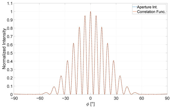
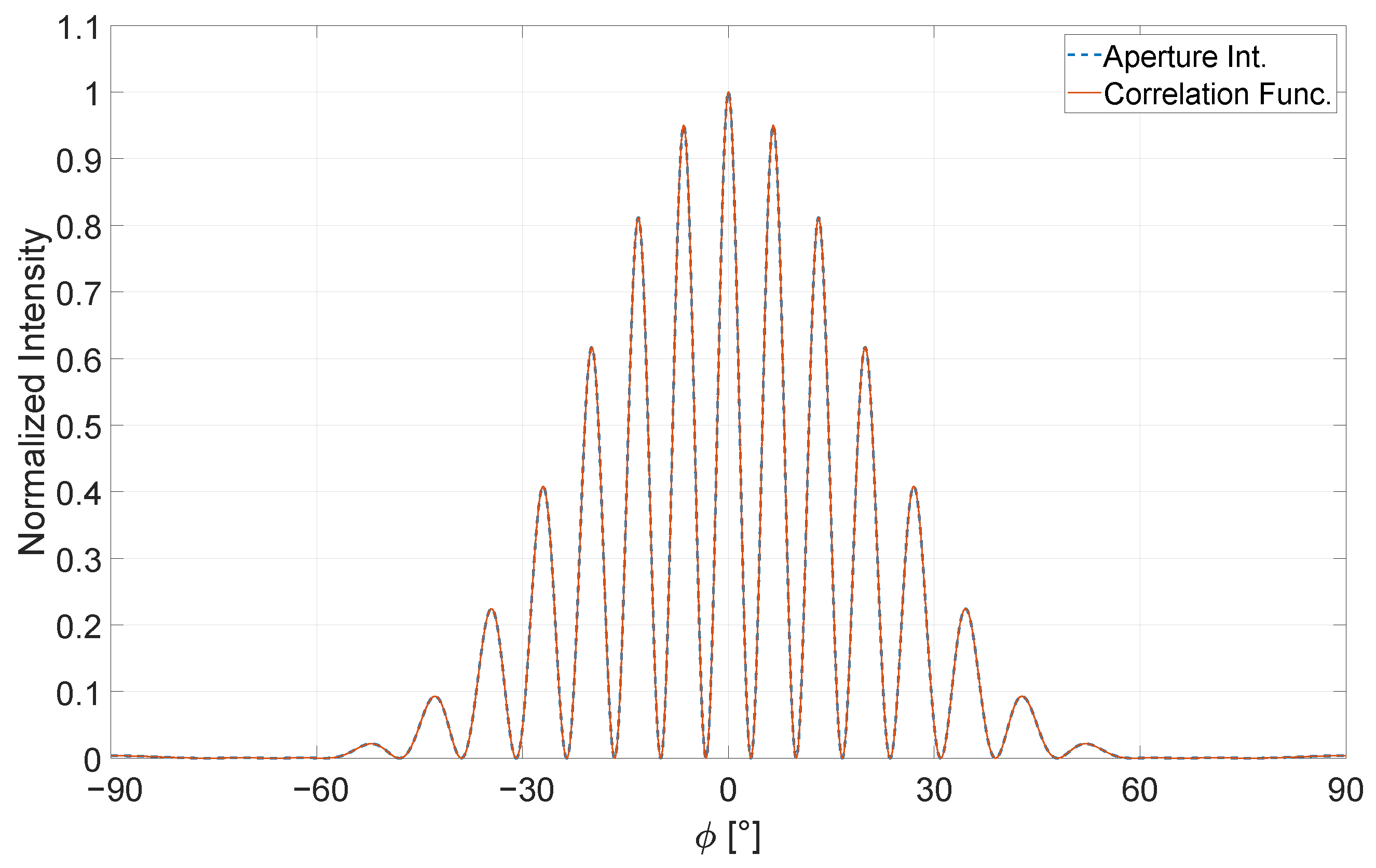
In case of Equation (7), D corresponds to the distance between the slits $|r_1-r_2|$, a describes the slit width, z describes the distance between the detection plane and the double-slit aperture and L corresponds to the distance between the light source and the double slit. The result is shown in Figure 1 for a fully coherent light source with a degree of coherence set to 1.

Figure 1. Direct comparison between the general aperture integral regarding [31,32] and the correction using the first-order correlation function [27,28,29,34,35]. Here, over an angular scale of $[-90°,90°]$ the normalized intensity of both equations is shown. Both equations display the same course within this interval. Here, the degree of coherence $\gamma (r_1,r_2,\tau )$ is set to $1.0$.

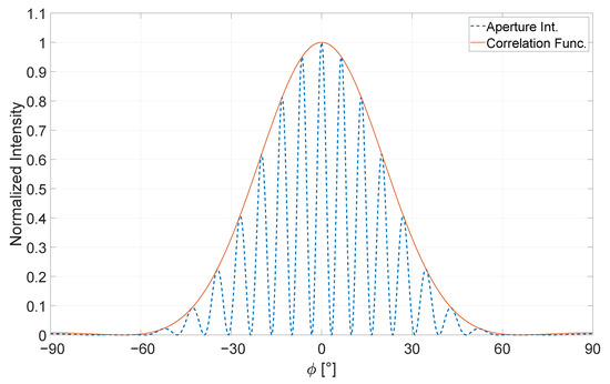
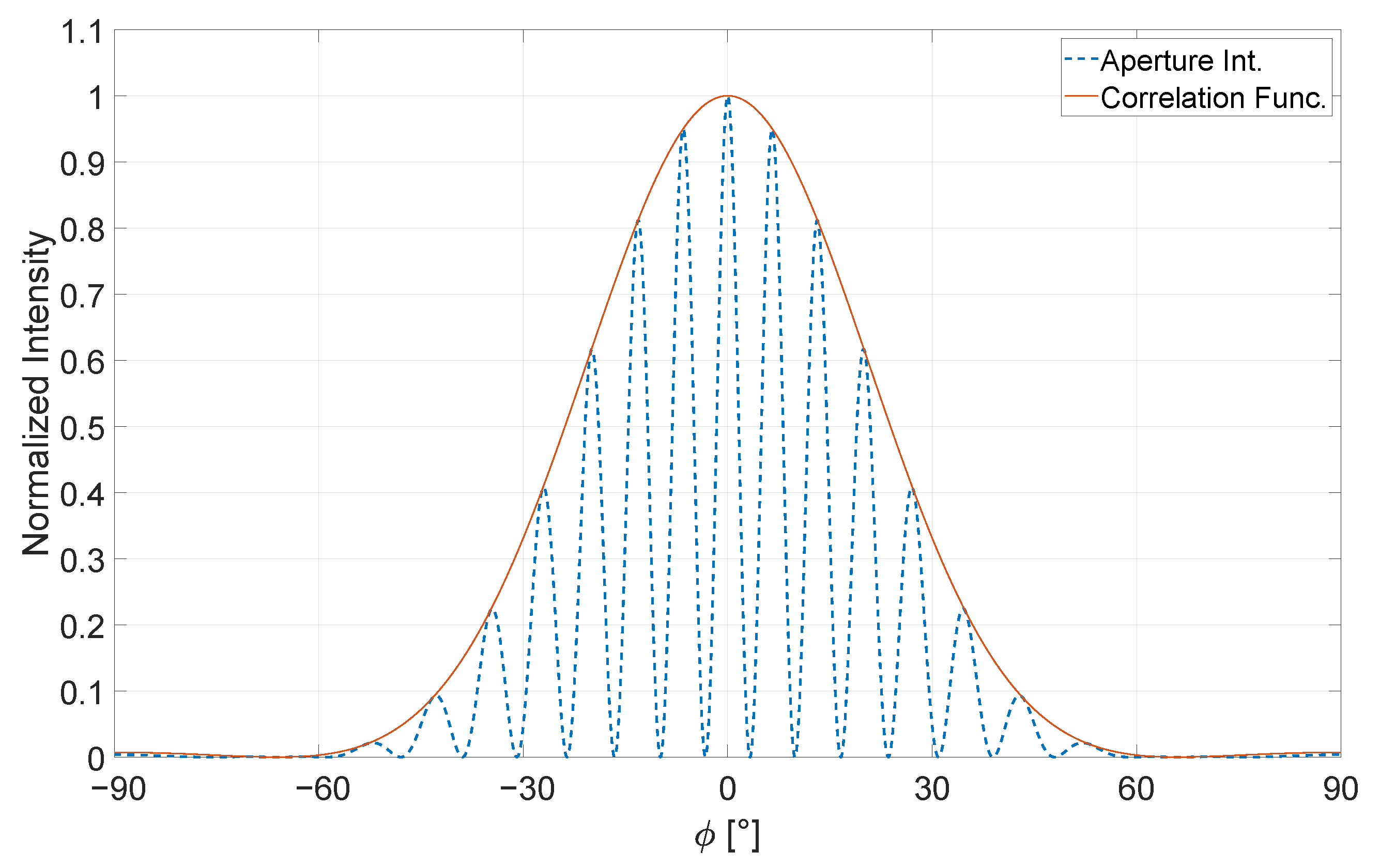
To evaluate the validity of this approach, we compare the classical aperture integral of the double slit with the modified version that includes a correction term accounting for partial incoherence. Figure 1 shows both the well-established aperture integral and the first-order correlation function under conditions of full coherence [31,32]. As expected, the two analytical results coincide. Figure 2 on the other hand, illustrates the effect of reducing the degree of coherence down to complete incoherence in this case. We observe that under conditions of complete incoherence, all interference patterns vanish within the orange curve. Thus, the first-order correlation function effectively describes the envelope of the aperture integral.

Figure 2. Direct comparison between the general aperture integral regarding to [31,32] and the correction using the first-order correlation function [27,28,29,34,35]. Here, over an angular scale of $[-90°,90°]$ the normalized intensity of both equations is shown. Both equations display the same course within this interval. Here, the degree of coherence $\gamma (r_1,r_2,\tau )$ is set to $0.0$.

3. Approximating Incoherent Monochromatic Light

This section provides a detailed introduction and description of the individual approximation methods. Each method is rigorously tested by varying key parameters to evaluate its performance. Finally, the results are compared across all methods to identify the most accurate approximation for incoherent blue light at 457 nm.

3.1. Simulation Setup

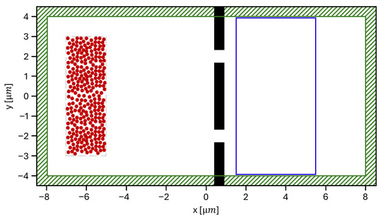
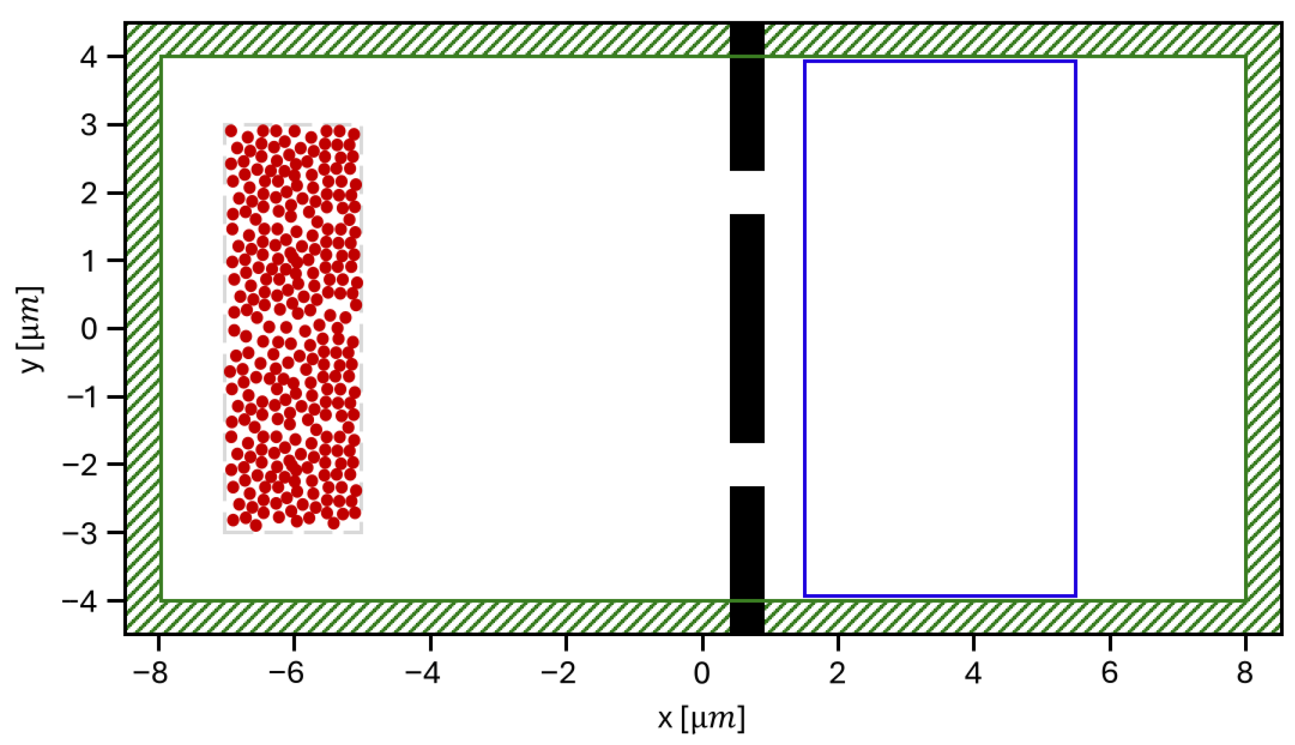
We begin by briefly introducing the simulation setup, which includes the incoherent light source and the double-slit aperture. The configuration is exemplified using the n-dipole emitter approach. The simulation domain has a total length of 17 $\mathsf{\mu }$m and a width of 9 $\mathsf{\mu }$m. The green-striped area along the edges of the simulation space represents the convolutional perfectly matched layer (CPML) boundary conditions, which are employed in FDTD simulations to absorb outgoing waves and minimize reflections [36,37,38]. These CPML layers reduce the effective simulation region by $0.5$ $\mathsf{\mu }$m on each side. The resulting effective simulation space thus measures 16 $\mathsf{\mu }$m in length and 8 $\mathsf{\mu }$m in width. The double-slit aperture is modeled using an arbitrary metallic material with ideal reflective properties. The geometry of the aperture includes a material thickness of $0.5$ $\mathsf{\mu }$m and extends entirely along the y-axis, such that wave propagation is only possible through the slits themselves. The slit structure is positioned between $0.5$ $\mathsf{\mu }$m and 1 $\mathsf{\mu }$m along the x-axis, with two openings centered at $-2$ $\mathsf{\mu }$m and 2 $\mathsf{\mu }$m along the y-axis, each having a width of $0.5$ $\mathsf{\mu }$m. A Near-to-Far-Field (NTFF) box is placed behind the slit structure, with dimensions of $(4\times 8)$ $\mathsf{\mu }$m. This box detects the transmitted field and converts it into an angular far-field distribution. Based on this setup, the parameters required to solve the first-order correlation function can be extracted. The slit separation D is 4 $\mathsf{\mu }$m, the slit width a is $0.5$ $\mathsf{\mu }$m, and the distance to the far-field detector z is set to 30 $\mathsf{\mu }$m in the simulations. This distance is sufficient to ensure an accurate far-field measurement, free from near-field effects.

3.2. Dipole Emitter for Incoherent Lighting

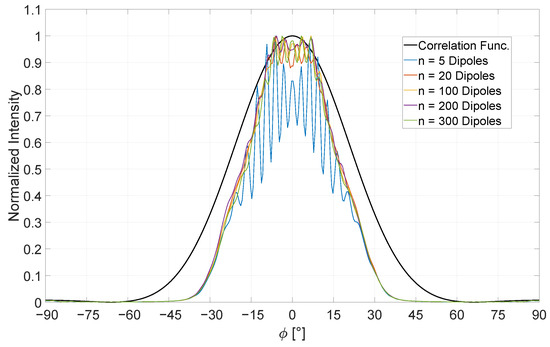
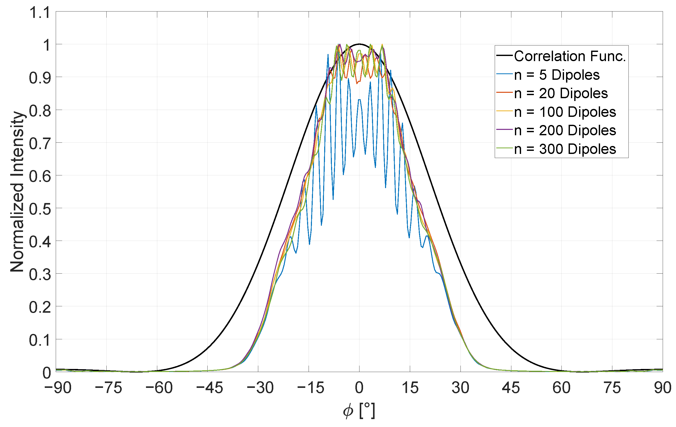
The first approximation examined in this section is the n-dipole approach, one of the most used techniques for incoherent light in FDTD simulations [23,38]. Within a defined region of the simulation domain, n-dipole sources are positioned. In this study, configurations with 5, 20, 100, 200, and 300 dipoles are investigated, distributed over a $(2\times 6)$ $\mathsf{\mu }$m area with a spacing of $6.5$ $\mathsf{\mu }$m to the double slit on average. This field is centered at the coordinate point $(-6,0)$ $\mathsf{\mu }$m shown in Figure 3. Each of the dipoles is assigned a randomized initial phase to minimize mutual self-interference among the sources [22,39,40]. For averaging the scattered fields 1000 simulations are performed to generate a single data set. It is observed that increasing the number of dipole sources improves agreement with the expected correlation behavior. This is illustrated in Figure 4. Indeed, the configuration with 300 dipole sources yields the closest match to the analytical solution. However, significant deviations from the idealized result remain. The simulated scattered light does not exhibit sufficient angular spread; on average, there is a discrepancy of approximately $10°$ between the expected illuminated solid angle and that obtained from the simulation. This deviation persists until the intensity reaches approximately 90% of its maximum. Beyond this threshold, strong fluctuations are observed in all cases, indicating an unknown residual degree of coherence inherent to the method. Although these interference pattern decrease with an increasing number of dipole sources, they are particularly pronounced within the angular range of $[-15°,15°]$. Consequently, while the method is suitable for approximating incoherent sources, it must be acknowledged that a certain degree of coherence remains intrinsic to this approach [22,23,38]. To mitigate these limitations, several adjustments can be made, although at the cost of increased computational effort. The number of dipole emitters can be further increased and distributed over a wider spatial region to introduce additional incident angles on the double slit. Moreover, the number of simulations used for statistical averaging can be expanded well beyond 1000 to improve agreement with the analytical model. In the subsequent section, the method is extended by introducing a spectral bandwidth to achieve greater accuracy.

Figure 3. Illustration of the two-dimensional simulation setup for the double slit with the example of the n-dipole approach. The double slit is placed between $0.5$ $\mathsf{\mu }$m and 1 $\mathsf{\mu }$m on the x-axis and fills the entire space along the y-axis. The slits are positioned at$-2$ $\mathsf{\mu }$m and 2 $\mathsf{\mu }$m with a width of $0.5$ $\mathsf{\mu }$m. The NTFF box is placed right behind the aperture with dimensions of $(4\times 8)$ $\mathsf{\mu }$m.

Figure 4. Simulation attempts with 5, 20, 100, 200 and 300 dipoles with randomized phase compared with the analytical calculation of the first-order correlation function on an angular scale between $[-90°,90°]$.

3.3. Dipole Emitter with Certain Bandwidth for Incoherent Lighting

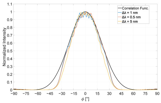
To improve this approach and align the averaged simulation results more closely with the analytical correlation function, several modifications are introduced. Real-world incoherent light sources are typically not monochromatic but consist of a spectrum of wavelengths. This spectral distribution is referred to as the spectral bandwidth of the source. Each wavelength component contributes to the dephasing of the individual dipoles due to differences in wavelength, leading to a randomized distribution of phase and amplitude along the wavefront. This means that a list of randomized values within the selected spectral bandwidth is generated. Each dipole is then assigned not only a randomized phase but also a slightly different wavelength within that bandwidth. Consequently, for n chosen dipoles, up to n distinct wavelengths can be assigned. The advantage of this approach lies in the fact that, in addition to phase randomization—which helps suppress interference effects—each dipole exhibits a slightly different angular scattering behavior due to its unique wavelength. This is particularly effective when each dipole is assigned a distinct wavelength. However, if the number of wavelengths within the bandwidth interval is reduced, the degree of residual coherence in the simulation may increase. This, in turn, results in a partial or complete loss of temporal and spatial coherence. In the FDTD framework, dipole emitters are typically modeled as point sources radiating light radially with defined spectral and polarization properties. For this extended n-dipole approach, the number of dipoles is again set to 300, as this configuration was found to yield the best agreement in the previous section. These sources are placed around the coordinate point $(-6,0)$ $\mathsf{\mu }$m. Despite these refinements, noticeable deviations from the analytical result remain. On average, the angular spread of the scattered field after passing through the double slit is approximately $10°$ too narrow compared to the correlation function, as illustrated in Figure 4. Additionally, a soft interference pattern is observed in the angular range $[-15°,15°]$, where none is expected. To further reduce coherence, the 300 dipole sources are assigned wavelength variations of $\Delta \lambda =0.5$ nm, $\Delta \lambda =1.0$ nm and $\Delta \lambda =5.0$ nm, respectively. These variations aim to enhance the degree of incoherence. Figure 5 presents the normalized intensity for each case across an angular spectrum of $[-90°,90°]$, with the analytical reference shown in black and the simulated variations in color. Compared to the n-dipole method discussed previously, this extended approach demonstrates clear improvements, particularly in areas where the original method exhibited weaknesses.

Figure 5. Simulation attempts with a certain bandwidth of $\Delta \lambda =0.5$ nm, $\Delta \lambda =1.0$ nm, $\Delta \lambda =5.0$ nm, for the 300 selected dipole emitter with randomized phase and amplitude compared with the analytical calculation of the first-order correlation function. This shows the scattered normalized intensity for the angular scale between $[-90°,90°]$.

In FDTD simulations, the addition of spectral bandwidth to the dipole sources prevents long-range and long-time interference between the emitted fields. In all tested cases, the illuminated angular range is broader and aligns with the analytical correlation function from an intensity level as low as 30%. Additionally, in the central peak around $0°$, a significant reduction in fluctuations is observed, indicating improved coherence suppression. The averaged simulation data for a spectral bandwidth of $\Delta \lambda =1.0$ nm shows the greatest overlap with the analytical reference. However, some limitations persist across all test cases. Below 30% of maximum intensity, noticeable deviations occur in the angular ranges $[-60°,-30°]$ and $[30°,60°]$. One possible remedy involves increasing the number of dipole sources and distributing them more widely across the simulation region in front of the double slit or aperture, thereby enabling a broader range of incident angles on the structure. A further challenge, also noted in the basic n-dipole model, remains: despite randomized phases and amplitudes, a residual degree of coherence persists due to the finite spectral bandwidth. This is particularly evident in the angular range $[-15°,15°]$, although clearly reduced compared to the previous approach, as shown in Figure 4 compared to Figure 5. To further mitigate these shortcomings, the statistical averaging process could be extended significantly beyond 1000 simulations, potentially yielding results with even closer agreement to the analytical solution. However, this expansion is strongly bounded on the computational capacity and simulation time. Furthermore, it is crucial to assess the required accuracy of the optical system under consideration. In particular, it must be evaluated whether variations in the intensity distribution of the LED are detrimental to the system performance or whether they have only a negligible impact on the resulting light distribution.

3.4. Cosine–Fourier Series Base Functions for Plane Waves

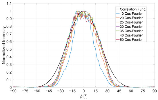
Considering the constraints in computational time and resource usage, both previously described dipole-based approaches offer potential for improvement. A notable advancement is provided by the Cosine–Fourier method, which reduces the number of randomized dipole sources to a single emitter [22,41]. In this approach, the dipole array is replaced by a single plane wave propagating perpendicularly toward the double slit. To incorporate stochastic behavior, Cosine–Fourier Series are embedded into the plane wave, effectively modulating it. The different basis functions introduce oscillations perpendicular to the direction of propagation, fragmenting the otherwise uniform wavefront into sections that interact with the double slit differently. As each partial wavefront deviates from its neighboring segment, the resulting scattering patterns vary. Across a set of m different base functions, the shape of the wavefront changes with each configuration. When conducting 1000 simulations, averaged post-process, there is potential for some wavefronts to repeat, thereby introducing a statistical distribution into the resulting diffraction pattern. This mimics the behavior of coherent or partially coherent light sources. Simulations are carried out with 10, 20, 25, 30, 35, 40 and 50 distinct Cosine–Fourier functions. These modifications are embedded using Equation (8) [41].

$$f_m\left(x\right)=\sqrt{{\displaystyle \frac{c_m}{L}}}\cos \left({\displaystyle \frac{m\pi x}{L}}\right),m=0,1,\dots ,M-1$$

(8)

This equation defines the amplitude profile of the source in the m-th simulation run, following the functional form depicted in Equation (8). Accordingly, M distinct Cosine–Fourier Series of the specified structure are employed. The parameter $c_m$ is defined as 1 for $m=0$, and 2 for all $m>0$. The variable L denotes the total width of the plane wave, which, in this case, corresponds to the simulation domain width of 8 $\mathsf{\mu }$m plus an additional 1 $\mathsf{\mu }$m reserved for PML boundary conditions. Furthermore, each Cosine–Fourier function is shifted in space to avoid repetition in modulation for a higher degree of randomization. The seven tested simulation sets are illustrated in the following. Figure 6 presents the simulation results in direct comparison with the analytical solution. The x-axis denotes the angular scale of the far-field in the interval $[-90°,90°]$, while the y-axis represents the normalized light intensity. Significant deviations from the analytical correlation function are observed, particularly for smaller numbers of Cosine–Fourier components. It can be observed that with 30 Cosine–Fourier components, the simulation results exhibit minimal further change. As shown in Figure 6, the averaged simulation data closely aligns with the analytical solution. However, notable discrepancies persist, particularly in the angular regions $[-60°,-30°]$ and $[30°,60°]$ at intensity levels below 30%. Moreover, within the central region $[-15°,15°]$, well-defined interference maxima are no longer present. Instead, the distribution appears rather coarse. A distinct peak around $-{13}^{°}$ on the left-hand side can be seen, which gradually decreases and then merges into the general trend of the analytical function. This pattern indicates that the residual degree of coherence has further decreased compared to the n-dipole method incorporating spectral bandwidth $\Delta \lambda$. Additionally, the computational effort required for these 1000 simulations is approximately half that of the previous approach. To further improve the agreement between the simulated and analytical results, a larger number of Cosine–Fourier components could be employed in combination with an increased number of simulations for statistical averaging. A sufficiently large dataset may suppress the unwanted peak at $13°$ on the left side and lead to an even closer match with the analytical correlation function.

Figure 6. Simulation attempts with 10, 20, 25, 30, 35, 40 and 50 different Cosine–Fourier functions compared with the analytical calculation of the first-order correlation function. The scattered normalized intensity is shown on an angular scale between $[-90°,90°]$.

3.5. Randomized Gaussian Beam Incident Angles

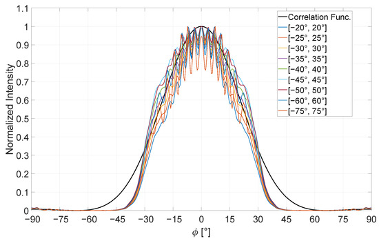
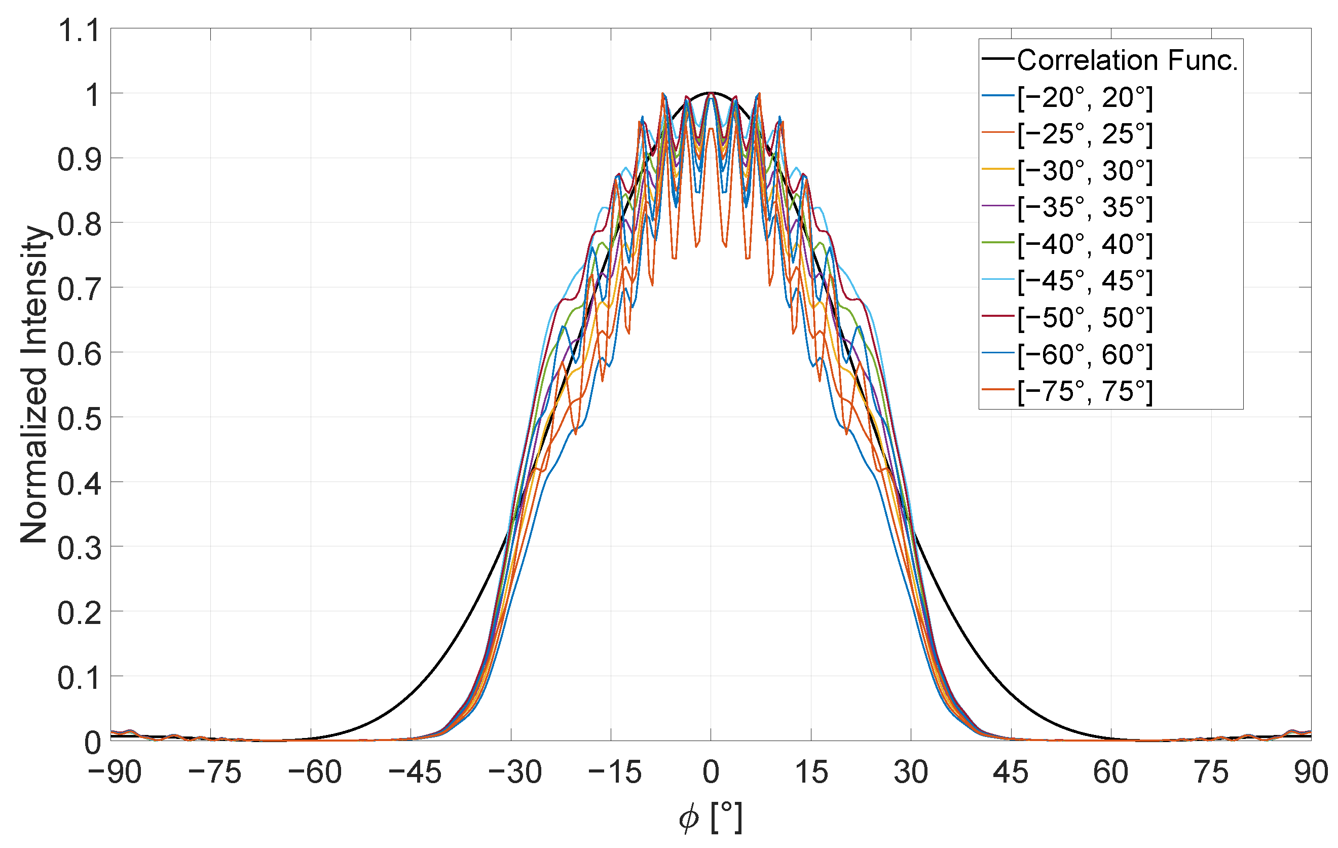
Another approach for realizing incoherent light sources involves using a Gaussian beam as the emitter, following the method described by Moreno [17]. Unlike the approach in which the polarization state of the Gaussian beam is varied, this method maintains a constant polarization while varying the angle of incidence. Since only a single source—namely the Gaussian beam—propagates toward the double slit in each simulation, there is no need to implement a randomized phase to avoid self-interference. Each individual simulation yields a fully coherent diffraction pattern; however, the intensity distribution varies with angle due to the differing incident directions. By randomizing the incident angle within a predefined interval and averaging the results of 1000 simulations, the aim is to produce a diffraction pattern representative of an incoherent light source – one that closely matches the analytically derived solution. To investigate this method, nine angular intervals were defined: $\pm 20°$, $\pm 25°$, $\pm 30°$, $\pm 35°$, $\pm 40°$, $\pm 45°$, $\pm 50°$, $\pm 60°$, and $\pm 70°$. The averaged simulation results are presented in Figure 7, directly compared to the analytical prediction. The figure shows the normalized light intensity plotted over the angular range of $[-90°,90°]$.

Figure 7. Simulation attempts with the selected intervals of $\pm 20°$, $\pm 25°$, $\pm 30°$, $\pm 35°$, $\pm 40°$, $\pm 45°$, $\pm 45°$, $\pm 60°$ and $\pm 70°$ for the Gaussian beam incident compared with the analytical calculation of the first-order correlation function. The scattered normalized intensity for the angular scale between [$-\pm 90°,\pm 90°$].

In all cases, an expanded illuminated region is observed above an intensity threshold of 30%. Below this threshold, the angular intensity profile narrows, as seen in previous approaches, and deviates from the analytical prediction in the intervals of $[-60°,-30°]$ and $[30°,60°]$. Since each simulation involves a fully coherent Gaussian beam incident on the double slit, each individual result yields a distinct diffraction pattern tailored to the beam’s angle of incidence. In this regard, the Gaussian method differs fundamentally from the dipole-based approaches. However, it proves to be approximately twice as time efficient. Centered around the origin in an interval $[-15°,15°]$, we also observe interference features that closely follow the analytical intensity profile. This indicates the presence of a residual degree of coherence. Increasing the angular interval does not significantly improve the outcome. However, increasing the number of simulations well beyond 1000 may help further reduce interference artifacts. Notably, the resulting intensity distribution appears highly symmetric about $0°$ degree, despite the randomized order of incidence angles. Overall, this method also proves suitable for approximating incoherent light behavior in diffraction simulations.

4. Evaluation and Discussion

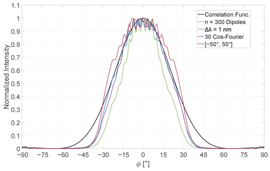
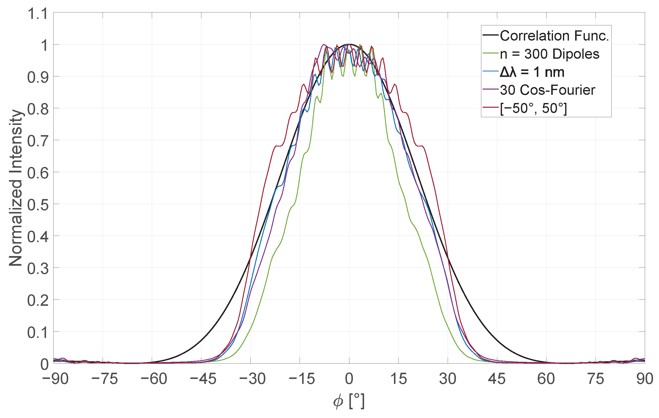
Finally, the results of the four presented methods for approximating incoherent light sources are evaluated and compared with one another. As a reference, we employed the first-order correlation function as outlined in Section 2, incorporating it into the aperture integral. The degree of coherence, denoted as $\gamma$, serves as the critical parameter within this function. By setting $\gamma =0$, we analytically model a completely incoherent light source, enabling the representation of the angular scattering distribution across a range from $[-{90}^{°},{90}^{°}]$. To ensure consistency across all datasets, the simulated intensity values are normalized. First, we evaluate the dipole approach [36,37,38]. During the simulation, the resulting wavefront propagates towards the double slit, generating a transmission field with a characteristic scattering pattern. This process is repeated 1000 times, and the averaged result is considered statistically robust for the intended comparison. As shown in Section 3, the configuration with the highest number of dipole emitters yields the closest agreement with the analytical reference. However, the green curve in Figure 8 reveals significant deviations from the ideal behavior. In summary, while this technique provides a reasonable approximation of incoherent light behavior, it exhibits clear limitations and deviations from the analytical model. To enhance its accuracy, the number of dipole sources can be increased, and their spatial distribution can be broadened in front of the aperture. Furthermore, a larger set of simulations for statistical averaging would likely yield results that converge more closely with the analytical prediction. To enhance the n-dipole emitter method, we introduce a refined approach that aligns the model more closely with real, monochromatic light sources. Even ideally monochromatic incoherent light sources inherently exhibit a finite spectral bandwidth. This physical characteristic is now incorporated into the existing configuration of 300 dipole emitters. Various bandwidths were investigated, but the most accurate match to the analytical result was observed for a spectral width of $1.0$ nm. The corresponding dataset is represented by the blue curve in Figure 8. In this case, the averaged simulation data aligns with the analytical prediction above an intensity threshold of 30%. Below this threshold, however, significant deviations persist, particularly in the angular ranges of $[-60°,-30°]$ and $[30°,60°]$. Additionally, interference patterns around the origin within the interval $[-15°,15°]$ are less pronounced and more closely follow the analytical behavior. When comparing both n-dipole emitter methods, it becomes evident that the inclusion of spectral band width $\Delta \lambda$ offers a notably improved approximation of incoherent light behavior.

Figure 8. Visualization of the results for each approximation method compared with the analytical calculation in black for fully incoherent light. Green represents the averaged simulation data form the n-dipole approach using 300 dipoles. Blue shows the expansion of this approach implementing a bandwidth of $\Delta \lambda =1.0$ nm. Purple corresponds to the averaged simulation data for a set of 30 different Cosine–Fourier functions. The red line shows the result for the Gaussian beam incidence within an interval of $[-50°,50°]$. Each data is averaged with 1000 simulations to receive a meaningful scope and a valid result.

Nevertheless, a slight degree of residual coherence remains visible at the peak intensity. To further refine this method, the spatial distribution of dipole emitters could be expanded across a broader region in front of the double slit, and the number of simulation runs used for averaging could be increased beyond 1000, thereby improving convergence toward the analytical result. Both dipole-based methods require significantly greater computational effort compared to the approximation approaches using single sources, primarily due to the large number of sources—300 dipole emitter—used in the simulation, which substantially increases computation time. To mitigate this, the subsequent methods reduce the number of sources to a single emitter. In the Cosine–Fourier method, a plane wave is employed that propagates perpendicularly toward the double slit [41]. The wavefront is modulated using different Cosine–Fourier functions, introducing oscillations orthogonal to the direction of propagation, which distort the wavefront. As a result, partial wavefronts deviate in shape from their neighboring segments, thereby simulating a form of incoherence. Across 1000 simulations, this procedure introduces up to 50 different Cosine–Fourier functions. The purple curve in Figure 8 illustrates the resulting averaged simulation data. Compared to the blue curve, the purple curve displays a slightly narrower angular distribution relative to the analytical solution. A noticeable peak appears around $-13°$, followed by a gradual decay marked by minor fluctuations, eventually aligning with the analytical result at larger angles. These fluctuations suggest residual interference effects, indicating a remaining degree of partial coherence. As with the previous methods, significant deviations from the ideal model are also observed in the angular intervals $[-60°,-30°]$ and $[30°,60°]$. To further reduce discrepancies and better match the analytical prediction, an increased number of simulation runs for averaging could be considered. Since this method operates at approximately 50% of the computational cost compared to the n-dipole emitter methods, extending the simulation scope is computationally feasible. Another approach involves the implementation of Gaussian beams, as described in [17]. However, the pronounced peak observed at approximately $-13°$ constitutes a distinctive feature that does not occur in any of the other investigated methods. A plausible explanation for this behavior lies in the modulation of the plane wave by the Cosine–Fourier series. To avoid repetitive patterns inherent to these series, the modulation functions are laterally shifted. This spatial shift may, in turn, influence the averaged result and thus provide an explanation for the observed asymmetry in the light distribution. Similarly to the Cosine–Fourier method utilizing plane waves, this approach employs only a single source, resulting in a comparable computational time frame. However, in contrast to the previous method, the angle of incidence is varied randomly within a defined interval. The incoherence is thereby simulated through the stochastic variation of the incident angle. A total of 1000 simulations are performed and subsequently averaged to reproduce a scattering behavior that resembles that of an incoherent light source. Figure 8 presents the outcome for an angular interval of $[-50°,50°]$, depicted in dark red. In the angular regions of $[-60°,-30°]$ and $[30°,60°]$, the resulting scattering profile appears narrower than the analytical reference. Nevertheless, this behavior is consistent with the trends observed in the other approximation methods. Beyond an intensity threshold of 30%, the scattering profile becomes broader than the analytical prediction but aligns with it at the central peak, albeit with pronounced fluctuations. These fluctuations indicate a significant degree of residual coherence. When considering only the angular distribution, however, this method remains a viable approximation for simulating incoherent light. An increased number of simulations for averaging could help reduce these interference effects near the peak. Nonetheless, due to the intrinsic coherence of the individual Gaussian beams, such artifacts are expected to persist to some extent. Figure 8 provides a direct comparison of all approximation methods with the analytical solution, displaying normalized intensity on the y-axis and the angular scale ranging from $[-90°,90°]$ on the x-axis. In addition to the interference phenomena centered around the origin, a consistent deviation appears across all investigated methods in the angular ranges of $[-60°,-30°]$ and $[30°,60°]$. While the central interference effects can be attributed to residual coherence inherent to the respective light sources, this specific angular deviation is not directly influenced by the coherence properties within the FDTD simulations. A possible explanation for the discrepancy between the simulation results and the analytical correlation function may lie in the configuration and placement of the NTFF box, as well as the temporal boundaries of the simulations. All simulations are run until the wave has propagated 25 $\mathsf{\mu }$m through the computational domain. When using spatially extended sources, such as the dipole emitter methods, a broader angular range in the transmitted field can be accessed. This is due to the fact that each dipole would then be oriented differently with respect to the double slit, thus altering the angular distribution of scattered light. The NTFF box is placed symmetrically behind the double slit and spans an area of $(8\times 4)$ $\mathsf{\mu }$m. If the simulation domain were enlarged, the NTFF box geometry could also be proportionally increased. This would ensure a uniform propagation distance to the far-field, even for higher angular components, similar to the $0°$ direction. Such a modification in the NTFF box geometry might influence the far-field behavior for larger angles and lead to minor corrections in the observed angular distribution. Nevertheless, the current configuration is chosen in accordance with established practices found in the literature [22,23,36,37,38], in which half of the NTFF box extends into the transmissive field and the other half into the reflective field. Since only the transmitted field is relevant for our analysis, the box is oriented accordingly. Regarding the simulation duration the temporal setup is sufficient, given that the entire spatial domain measures only 16 $\mathsf{\mu }$m. The full two-dimensional simulation setup is illustrated again in Figure 3. However, the fact that all methods exhibit the same inaccuracies in these angular regions suggests a more fundamental limitation. Despite their randomized nature, each source type used in these simulations remains internally coherent due to the nature of FDTD modeling. All methods presented here have their merits and broadly reproduce the general features of the analytical solution. However, in direct comparison, the dipole method incorporating spectral bandwidth and the approach involving modulation of the plane wave via Cosine–Fourier functions yield the most convincing results. These two methods exhibit strong agreement with the analytical model, both in the flanks of the angular distribution and at the central peak within the interval $[-15°,15°]$ around the origin. Only minor fluctuations are observed in these regions, indicating a very low degree of residual coherence—precisely the objective of this section: to identify methods that closely approximate fully incoherent light sources. In contrast, the conventional n-dipole emitter method described in the literature [36,37,38] shows significant deviations from the first-order correlation function and fails to adequately cover the full angular spectrum in both width and amplitude. Moreover, this method retains a substantial level of residual coherence, which manifests as pronounced interference effects at the central peak. Considering the computational demands, this approach proves to be relatively inefficient. Similarly, the Gaussian beam method based on varying incidence angles is found to be unsuitable. Since each beam remains fully coherent, averaging across simulations still results in strong interference effects. These appear already on the flanks at approximately $[-25°,25°]$ and intensify toward the central region. In conclusion, among the four investigated approaches, two have emerged as particularly promising approximation models for incoherent light sources. These methods offer a robust basis for future simulations and further theoretical studies.

5. Conclusions

Using the various methods presented, it is possible to approximate incoherent light sources. In this study, these approaches were applied specifically to monochromatic light with a fixed wavelength of 457 nm across all simulation series. Building upon the n-dipole emitter method [23,38], several additional approaches were developed and comparatively analyzed. Within each method, key parameters were systematically varied to assess under which conditions the numerical results most closely matched the analytical solution. To ensure a reliable and analytically tractable reference, a double-slit geometry was employed. This configuration offers the advantage of being solvable both through the first-order correlation function [20,27,28,29], and via the classical aperture integral formulation [31]. While both analytical models yield identical results for fully coherent light, the correlation function allows for the incorporation of partial coherence via the degree of coherence parameter. In the limit of complete incoherence, this model serves as a valid theoretical reference and is used as the benchmark for evaluating the approximation methods. The investigated models included the n-dipole emitter approach [23,28], an extension incorporating spectral bandwidth [20,27,28,29], a computationally efficient method using a plane wave modulated by Cosine–Fourier Series [22], and a Gaussian beam incident on the slit at varying angles. All methods aimed to reproduce the far-field behavior of an incoherent light distribution. However, in all cases, coherence-related artifacts were observed in the upper 90% intensity range, indicating a residual degree of coherence across all methods. These effects could potentially be minimized further by increasing the number of simulations contributing to the averaged results. Enlarging the dataset is expected to suppress such fluctuations. A more pronounced deviation was consistently observed in the low-intensity range at larger scattering angles, typically beyond $30°$ to $60°$, where all numerical results significantly diverged from the analytical model. Here, too, expanding the simulation dataset could improve accuracy within the approximation. In summary, all methods evaluated are capable of approximating incoherent light to some extent. Among them, the n-dipole method and the Cosine–Fourier-modulated plane wave approach yielded the most reliable results under the given conditions. The degree of incoherence could further be enhanced by introducing multiple wavelengths and averaging over them, thereby increasing not only the simulation volume but also the spectral bandwidth, which inherently reduces coherence. This perspective points toward future investigations, where the methods demonstrated here may be extended to simulate white-light LEDs using a polychromatic approximation.

References

- Nair, G.B.; Dhoble, S.J. The Fundamentals and Applications of Light-Emitting Diodes: The Revolution in the Lighting Industry; Woodhead Publishing: Sawston, UK, 2020. [Google Scholar]
- Sanderson, S.W.; Simons, K.L. Light emitting diodes and the lighting revolution: The emergence of a solid-state lighting industry. Res. Policy 2014, 43, 1730–1746. [Google Scholar] [CrossRef] [Scilit]
- Cole, M.; Clayton, H.; Martin, K. Solid-state lighting: The new normal in lighting. IEEE Trans. Ind. Appl. 2014, 51, 109–119. [Google Scholar] [CrossRef] [Scilit]
- Hong, G.; Gan, X.; Leonhardt, C.; Zhang, Z.; Seibert, J.; Busch, J.M.; Bräse, S. A brief history of OLEDs—Emitter development and industry milestones. Adv. Mater. 2021, 33, 2005630. [Google Scholar] [CrossRef] [Scilit] [PubMed]
- Sasabe, H.; Kido, J. Development of high performance OLEDs for general lighting. J. Mater. Chem. C 2013, 1, 1699–1707. [Google Scholar] [CrossRef] [Scilit]
- Buckley, A. Organic Light-Emitting Diodes (OLEDs): Materials, Devices and Applications; Elsevier: Amsterdam, The Netherlands, 2013. [Google Scholar]
- Supran, G.J.; Shirasaki, Y.; Song, K.W.; Caruge, J.-M.; Kazlas, P.T.; Coe-Sullivan, S.; Andrew, T.L.; Bawendi, M.G.; Bulović, V. QLEDs for displays and solid-state lighting. MRS Bull. 2013, 38, 703–711. [Google Scholar] [CrossRef] [Scilit]
- Choi, M.K.; Yang, J.; Hyeon, T.; Kim, D.-H. Flexible quantum dot light-emitting diodes for next-generation displays. npj Flex. Electron. 2018, 2, 10. [Google Scholar] [CrossRef] [Scilit]
- Lin, Q.; Zhu, Y.; Wang, Y. Flexible quantum dot light-emitting device for emerging multifunctional and smart applications. Adv. Mater. 2023, 35, 2210385. [Google Scholar] [CrossRef] [Scilit]
- Leary, G.; Switzer, G.; Kuntz, G.; Kaiser, T. Comparison of xenon lamp-based and LED-based solar simulators. In Proceedings of the IEEE 43rd Photovoltaic Specialists Conference (PVSC), Portland, OR, USA, 5–10 June 2016; IEEE: Piscataway, NJ, USA, 2016; pp. 3062–3067. [Google Scholar]
- Khan, N.; Abas, N. Comparative study of energy saving light sources. Renew. Sustain. Energy Rev. 2011, 15, 296–309. [Google Scholar] [CrossRef] [Scilit]
- Kloppenburg, G.; Wolf, A.; Lachmayer, R. High-resolution vehicle headlamps: Technologies and scanning prototype. Adv. Opt. Technol. 2016, 5, 147–155. [Google Scholar] [CrossRef] [Scilit]
- Rizvi, S.; Knöchelmann, M.; Ley, P.-P.; Lachmayer, R. Survey of on-road image projection with pixel light systems. In Photonics, Devices, and Systems VII; SPIE: Bellingham, WA, USA, 2017; pp. 257–263. [Google Scholar]
- Moreno, I. Introduction to Metalens Optics; IOP Publishing: Bristol, UK, 2024. [Google Scholar]
- Mehta, D.S.; Saxena, K.; Dubey, S.K.; Shakher, C. Coherence characteristics of light-emitting diodes. J. Lumin. 2010, 130, 96–102. [Google Scholar] [CrossRef] [Scilit]
- Halder, A.; Turunen, J. Spectral coherence of white LEDs. Photonics Res. 2022, 10, 2460–2470. [Google Scholar] [CrossRef] [Scilit]
- Moreno, I.; Sun, C.-C. Modeling the radiation pattern of LEDs. Opt. Express 2008, 16, 1808–1819. [Google Scholar] [CrossRef] [Scilit] [PubMed]
- Moreno, I. Spatial distribution of LED radiation. In Proceedings of the International Optical Design Conference, Vancouver, BC, Canada, 4–8 June 2006; SPIE: Bellingham, WA, USA, 2006; pp. 378–384. [Google Scholar]
- Sun, C.-C.; Chen, C.-Y.; He, H.-Y.; Chen, C.-C.; Chien, W.-T.; Lee, T.-X.; Yang, T.-H. Precise optical modeling for silicate-based white LEDs. Opt. Express 2008, 16, 20060–20066. [Google Scholar] [CrossRef] [Scilit] [PubMed]
- Goodman, J.W. Statistical Optics; John Wiley & Sons: Hoboken, NJ, USA, 2015. [Google Scholar]
- Gerry, C.; Knight, P. Introductory Quantum Optics; Cambridge University Press: Cambridge, UK, 2004. [Google Scholar]
- Oskooi, A.F.; Roundy, D.; Ibanescu, M.; Bermel, P.; Joannopoulos, J.D.; Johnson, S.G. MEEP: A flexible free-software package for electromagnetic simulations by the FDTD method. Comput. Phys. Commun. 2010, 181, 687–702. [Google Scholar] [CrossRef] [Scilit]
- Taflove, A.; Oskooi, A.; Johnson, S.G. Advances in FDTD Computational Electrodynamics: Photonics and Nanotechnology; Artech House: New York, NY, USA, 2013. [Google Scholar]
- Park, C.; Shin, J.M.; Kim, S.; Park, J.; Jang, M.S. Fast and rigorous electromagnetic simulation of dipole emission in a periodically corrugated LED structure based on diffraction tracking. In Proceedings of the MRS Fall Meeting, Boston, MA, USA, 29 November–2 December 2021; Materials Research Society: Warrendale, PA, USA, 2021. [Google Scholar]
- Qi, B. True randomness from an incoherent source. Rev. Sci. Instrum. 2017, 88, 113101. [Google Scholar] [CrossRef] [Scilit]
- Lauterborn, W.; Kurz, T.; Wiesenfeldt, M. Kohärente Optik; Springer: Berlin/Heidelberg, Germany, 2013. [Google Scholar]
- van Cittert, P.H. Die wahrscheinliche Schwingungsverteilung in einer von einer Lichtquelle direkt oder mittels einer Linse beleuchteten Ebene. Physica 1934, 1, 201–210. [Google Scholar] [CrossRef] [Scilit]
- Zernike, F. The concept of degree of coherence and its application to optical problems. Physica 1938, 5, 785–795. [Google Scholar] [CrossRef] [Scilit]
- Pearson, B.J.; Ferris, N.; Strauss, R.; Li, H.; Jackson, D.P. Measurements of slit-width effects in Young’s double-slit experiment for a partially-coherent source. OSA Contin. 2018, 1, 755–763. [Google Scholar] [CrossRef] [Scilit]
- Pieper, K.; Bergmann, A.; Dengler, R.; Rockstuhl, C. Visualizing and manipulating the spatial and temporal coherence of light with an adjustable light source in an undergraduate experiment. Eur. J. Phys. 2019, 40, 055302. [Google Scholar] [CrossRef] [Scilit]
- Hecht, E. Optik; De Gruyter: Berlin, Germany, 2023; ISBN 3111025594. [Google Scholar]
- Gobrecht, H.; Eichler, H.-J.; Bergmann, L.; Schaefer, C. Optik; De Gruyter: Berlin, Germany, 2019; ISBN 978-3-11-171061-7. [Google Scholar]
- Glauber, R.J. The quantum theory of optical coherence. Phys. Rev. 1963, 130, 2529. [Google Scholar] [CrossRef] [Scilit]
- Young, J. Elements of Optical Coherence Theory. Phys. Bull. 1984, 35, 73. [Google Scholar] [CrossRef] [Scilit]
- Beran, M.J. Theory of Partial Coherence; Prentice-Hall: Hoboken, NJ, USA, 1964. [Google Scholar]
- Elsherbeni, A.Z.; Demir, V. The Finite-Difference Time-Domain in Electromagnetics; SciTech Publishing: Raleigh, NC, USA, 2015. [Google Scholar]
- Roden, J.A.; Gedney, S.D. Convolution PML (CPML): An efficient FDTD implementation of the CFS–PML for arbitrary media. Microw. Opt. Technol. Lett. 2000, 27, 334–339. [Google Scholar] [CrossRef]
- Taflove, A.; Hagness, S.C.; Piket-May, M. Computational electromagnetics: The finite-difference time-domain method. In The Electrical Engineering Handbook; Elsevier: Burlington, MA, USA, 2005. [Google Scholar]
- Honnalli, N.V. Finite-Difference Time-Domain Simulations on Overgrown InGaN/GaN Multiple Quantum Well Light Emitting Diode. Master’s Thesis, NC State University, Raleigh, NC, USA, 2015. [Google Scholar]
- Bhalerao, M.V.; Sumathi, M.; Sonavane, S.S. Line of sight model for visible light communication using Lambertian radiation pattern of LED. Int. J. Commun. Syst. 2017, 30, e3250. [Google Scholar] [CrossRef] [Scilit]
- McCauley, A.P.; Rodriguez, A.W.; Joannopoulos, J.D.; Johnson, S.G. Casimir forces in the time domain: Applications. Phys. Rev. A 2010, 81, 012119. [Google Scholar] [CrossRef] [Scilit]
Disclaimer/Publisher’s Note: The statements, opinions and data contained in all publications are solely those of the individual author(s) and contributor(s) and not of MDPI and/or the editor(s). MDPI and/or the editor(s) disclaim responsibility for any injury to people or property resulting from any ideas, methods, instructions or products referred to in the content. |
© 2026 by the authors. Licensee MDPI, Basel, Switzerland. This article is an open access article distributed under the terms and conditions of the Creative Commons Attribution (CC BY) license.