


Abstract
In this paper, an improved architecture of time-window segmentation-based one-dimensional convolutional neural network (IATWSB-1D-CNN) is proposed for micro-displacement reconstruction in laser self-mixing interferometry (SMI). The improved architecture employs two convolutional layers, which effectively extract local features from SMI signals while reducing unnecessary network complexity. Batch Normalization layers are introduced to stabilize the feature distributions during training, while the Dropout layer is incorporated to prevent overfitting and improve the generalization performance of the network. The training stability and generalization performance of the network are enhanced by these architectural improvements. During the construction of the network, the continuous SMI signals are divided into a series of fixed-length signal sequences by the time-window segmentation, which are then used as network input samples. It improves network training efficiency. The displacement-related features can be progressively extracted from shallow to deep layers and enable the network to effectively learn displacement-related local features. This method establishes a nonlinear mapping between SMI signals and displacement, avoiding phase error accumulation in displacement reconstruction by phase unwrapping methods. Simulation results show that, under the noise-free condition and signal-to-noise ratios (SNRs) of 30 dB and 20 dB, the root mean square error (RMSE) values of the IATWSB-1D-CNN method are 0.032, 0.060, and 0.100, respectively, whereas the RMSE values of the phase unwrapping method are 0.049, 0.59, and 0.63, respectively. The stability of the IATWSB-1D-CNN method is further evaluated by independently training the network 30 times under the noise-free condition and SNRs of 30 dB and 20 dB. The RMSE values correspond to the coefficient of variation (CV) of 1.2%, 7.7%, and 9.4%, respectively. Experimental results show that the RMSE values of the IATWSB-1D-CNN and the phase unwrapping methods are 0.062 and 0.115, respectively. The RMSE values from 30 training trials correspond to the CV of 8.6%. These results demonstrate that the IATWSB-1D-CNN method exhibits good performance in reconstruction accuracy, efficiency and anti-noise capability, while maintaining stable and reproducible displacement reconstruction.
1. Introduction
SMI utilizes the interaction between optical feedback and the laser intracavity field, enabling target motion information to be directly encoded into the laser output signals [1]. Compared with traditional Michelson and Mach–Zehnder interferometers, SMI systems dispense with an additional reference optical path and feature a simple structure, low cost, strong self-collimation performance, and easy integration. Such advantages have enabled their widespread applications in micro-displacement measurement, vibration monitoring, biomedical detection, and industrial online inspection [2,3].
At present, SMI displacement reconstruction methods mainly include phase unwrapping methods and convolutional neural network (CNN) methods [4,5]. Among them, phase unwrapping methods have attracted extensive attention due to their ability to recover continuous phase information from wrapped SMI signals [6,7,8]. However, phase unwrapping methods rely heavily on high-quality SMI signals. When SMI signals are contaminated by speckle noise, quantization noise, and environmental disturbances, errors may occur in extrema detection and phase extraction, resulting in incorrect phase unwrapping and cumulative displacement reconstruction errors [9,10,11].
CNN adopts local receptive fields and weight sharing to automatically extract periodic fringes, peak-valley variations, and fringe jump features from SMI waveforms, and directly builds a nonlinear mapping between interferometric signals and target displacement, eliminating a series of intermediate steps such as extrema detection, phase extraction, and phase unwrapping [12,13,14,15]. Therefore, CNN has been widely adopted in vibration recognition, time-series signal analysis, and nonlinear regression tasks, offering a novel research direction for SMI displacement reconstruction [16,17]. Novac et al. presented the first integrated SMI sensor prototype embedded with neural networks [18]. Their embedded processing platform runs neural network inference, where the neural network reconstructs target displacement from incoming interferometric signals. Kou et al. developed a single-hidden-layer artificial neural network to discriminate the slope of SMI fringes [19]. The network uses extracted fringe waveforms as input features to distinguish left- and right-tilted fringes, achieving high discrimination accuracy under noisy and weak optical feedback conditions. Matha et al. [20] employed a convolutional neural network to reconstruct the target displacement directly from the single-channel SMI signal of a semiconductor laser; trained on periodic displacement patterns, the network generalized to different alignment conditions and setups. Siddiqui et al. employed two convolutional deep neural networks for SMI fringe detection under variable optical feedback [21]. Their workflow contains an automatic fringe labeling module, where the two CNNs perform fringe classification and target displacement reconstruction from speckle-contaminated interferometric signals.
Although the CNNs employed in the literature [13,20,21] have exhibited favorable nonlinear mapping capacity in this field, existing studies still have apparent limitations. Training on long time-series SMI signals imposes a heavy training load and leads to insufficient learning of local features [22]. Li et al. proposed a TWSB-1D-CNN method that divides the long SMI signal into multiple fixed-length local sequences before training. This approach avoids directly training the network on the entire long-time-series signal, thereby reducing the computational burden and enabling the network to focus on local features related to displacement reconstruction [23].
However, the training stability and generalization performance can also be affected by the network architecture in practical applications [24,25,26]. The training stability should be further improved by appropriate optimization of the network architecture; overfitting should also be avoided to enhance the generalization performance when trained on the limited training data [27]. Therefore, further improvement in network architecture is required to enhance training stability and generalization performance in the TWSB-1D-CNN method.
In this paper, the IATWSB-1D-CNN is proposed. First, the SMI signals are segmented using fixed-length time windows to construct network input samples, which improves the efficiency of network training. Second, the IATWSB-1D-CNN method is used to establish the nonlinear mapping between SMI signals and micro-displacement, enabling direct reconstruction of micro-displacement. Finally, the comparison of displacement reconstruction using the IATWSB-1D-CNN method and the phase unwrapping method is conducted. Simulations and experiments are conducted to verify the performance of the IATWSB-1D-CNN method. Quantitative comparisons between the two methods are conducted under the noise-free condition and SNRs of 30 dB and 20 dB based on reconstructed waveforms, scatter diagrams, and RMSE.
Furthermore, to verify the training stability of the IATWSB-1D-CNN method, the network is independently trained 30 times under each of the noise-free, 30 dB, and 20 dB conditions, and the dispersion of the resulting RMSE values is statistically evaluated using the standard deviation (SD) and the CV [28]. The results demonstrate that the IATWSB-1D-CNN method exhibits good performance in reconstruction accuracy, efficiency and anti-noise capability, while maintaining stable and reproducible displacement reconstruction. This study mainly demonstrates the feasibility of the proposed IATWSB-1D-CNN under the conditions investigated in this paper.
2. Theoretical Simulation and Analysis
This section initially introduces time-window segmented SMI signals and describes the network architecture of the IATWSB-1D-CNN and its convolutional layer features. Then, displacement reconstruction simulations are performed using the IATWSB-1D-CNN, and its reconstruction performance is compared with the phase unwrapping method. Finally, the RMSE values obtained from 30 independent training trials are statistically analyzed to verify the stability and repeatability of the IATWSB-1D-CNN.
2.1. Time-Window Segmented SMI Signals
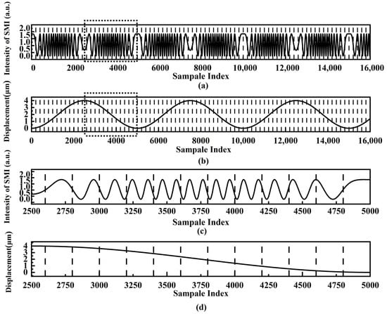
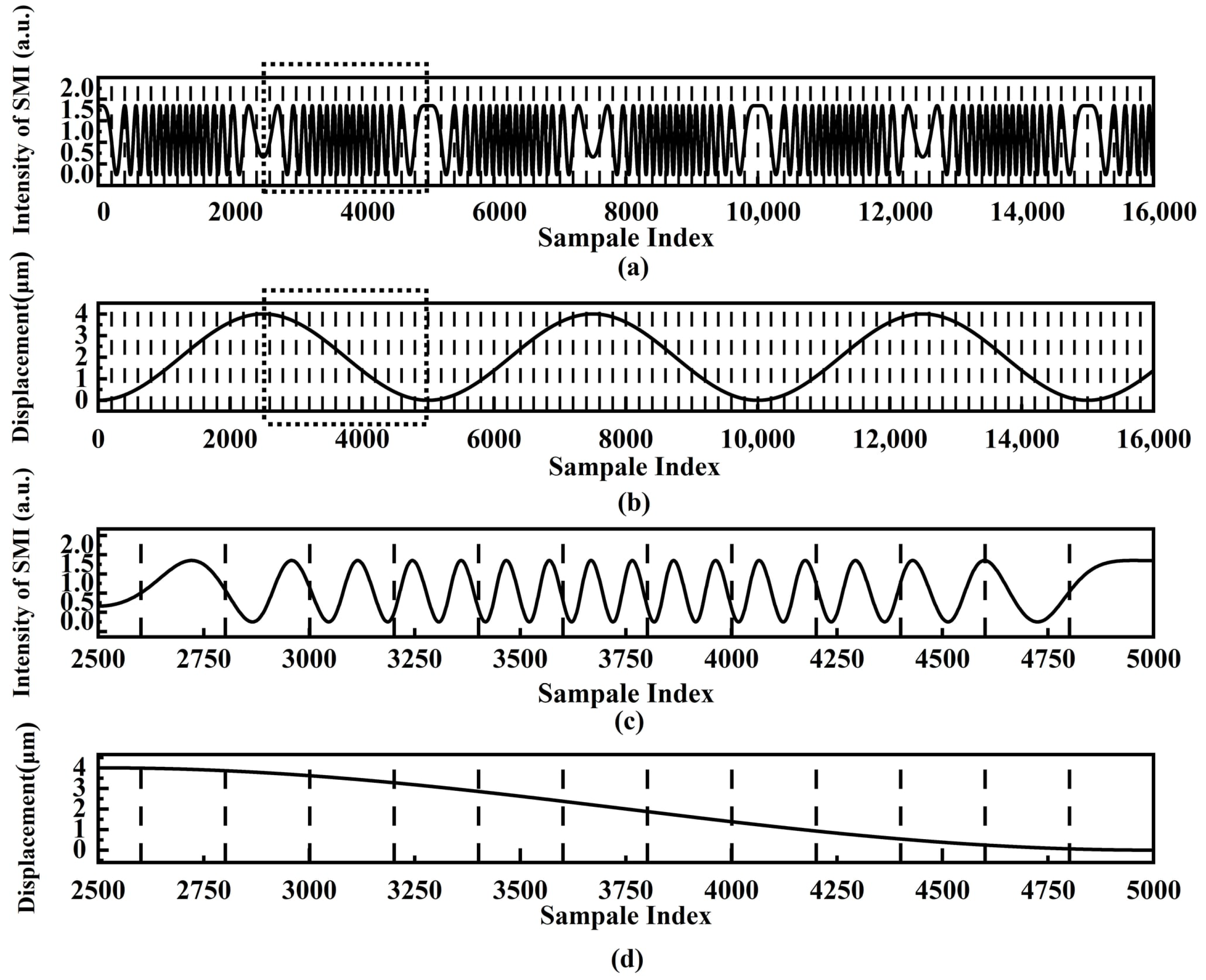
The continuous SMI signals are divided into multiple local signal sequences by the predefined window length. Figure 1 shows the time-window segmented SMI signals and displacement. As shown in Figure 1a, the black dotted lines indicate the segmentation boundaries of each local signal sequence. The original SMI signals are segmented into consecutive local signal sequences using the fixed-length window. Figure 1b shows the time-window segmented displacement corresponding to the segmented SMI signals, with the segmentation boundaries also marked by black dotted lines. Each local signal sequence is regarded as an independent input sample for the 1D-CNN, and its corresponding displacement value is used as the network output label. Figure 1c shows an enlarged view of the time-window segmented SMI signals in Figure 1a. Figure 1d shows an enlarged view of the segmented displacement in Figure 1b. The training efficiency of the 1D-CNN can be improved by the IATWSB-1D-CNN method.
Figure 1.
Time-window segmented SMI signals and displacement; (a) time-window segmented SMI signals marked by the vertical dotted lines; (b) time-window segmented displacement marked by the vertical dotted lines; (c) enlarged view of the segmented SMI signals marked by a dotted rectangle line shown in (a); (d) enlarged view of the segmented displacement marked by a dotted rectangle line shown in (b).
2.2. Network Architecture of the IATWSB-1D-CNN and Its Convolutional Layer Features
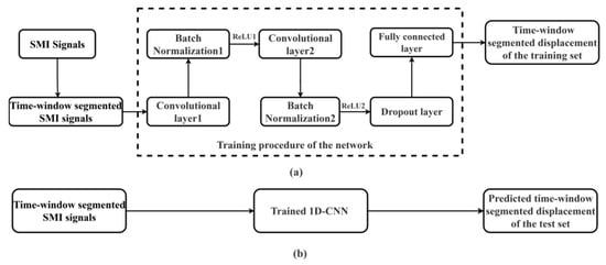
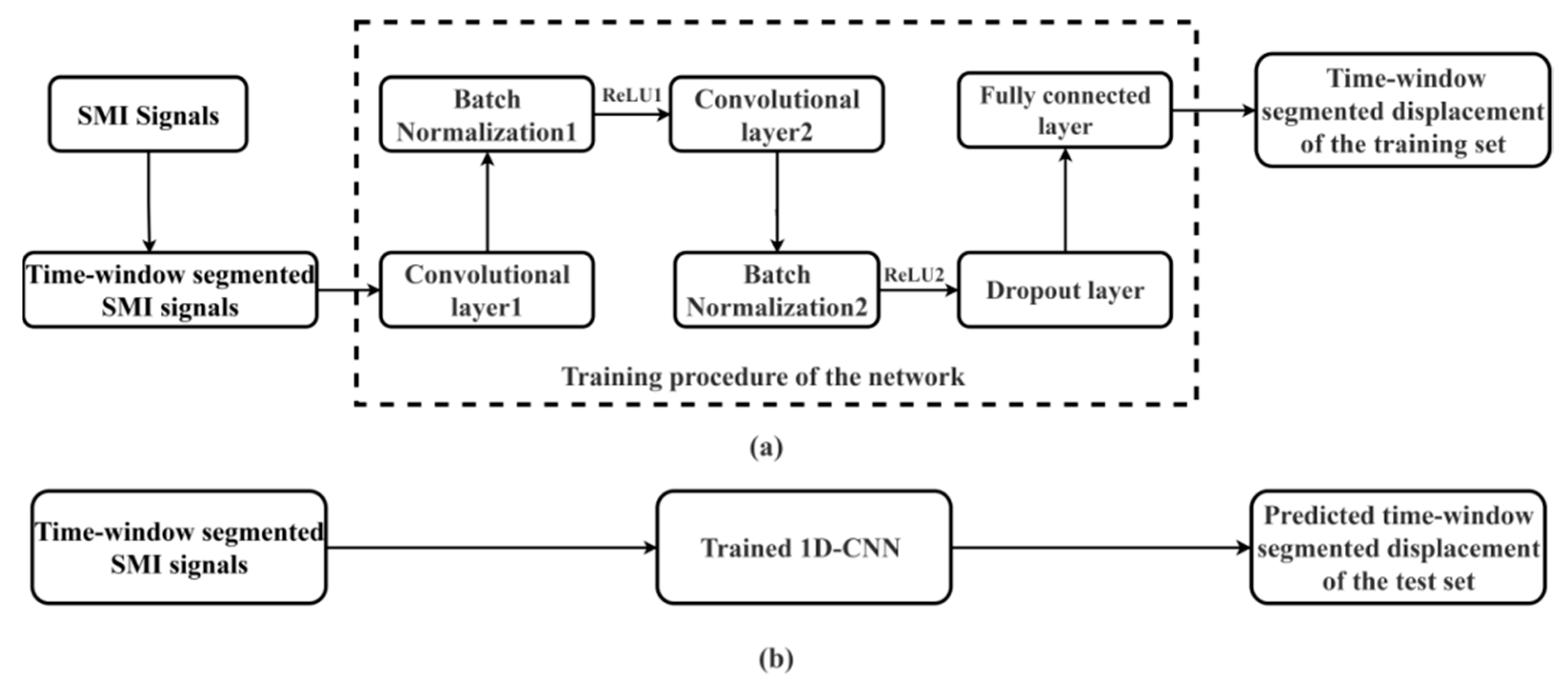
The IATWSB-1D-CNN is established for micro-displacement reconstruction in SMI. The overall structure of the IATWSB-1D-CNN is shown in Figure 2. Figure 2a shows the training stage, while Figure 2b describes the application stage. The detailed configuration of the network layers and the training hyperparameters is summarized in Table 1.
Figure 2.
Overall structure of the IATWSB-1D-CNN: (a) training procedure of the IATWSB-1D-CNN; (b) application procedure of the IATWSB-1D-CNN. ReLU: Rectified linear unit.
Table 1.
Network architecture and training hyperparameters of the IATWSB-1D-CNN.
As shown in Figure 2a, the network training process consists of two parts: SMI signal pre-processing and input and IATWSB-1D-CNN training. The network architecture employs two convolutional layers to effectively extract local temporal features from one-dimensional SMI signals while maintaining a simple network structure and reducing computational complexity.
Firstly, in the stage of SMI signal pre-processing and input, the continuous SMI signals are divided into fixed-length signal sequences by the time-window segmentation method. Subsequently, the time-window segmented SMI signals are input into the training procedure of the network. In the stage of IATWSB-1D-CNN training, the input samples are processed by the first convolutional layer, where local features of the SMI signals are automatically extracted through the local receptive fields and weight sharing of the convolution kernels. The extracted features are passed to the first Batch Normalization layer to normalize the feature distribution and then fed into the first ReLU activation layer [29] to introduce nonlinear representation capability. The features are subsequently fed into the second convolutional layer for further extraction of higher-level features. The output of the second convolutional layer is normalized by the second Batch Normalization layer and activated by the second ReLU layer to enhance the nonlinear feature representation. In both Batch Normalization layers, the learnable parameters are then used to rescale and shift the activations. The feature distribution can be stabilized and the network training can also be facilitated [30].
The extracted high-order features are then passed to the Dropout layer, where a fraction of neurons is randomly deactivated during training to reduce excessive co-adaptation among neurons, thereby preventing overfitting and improving the generalization of the network [27]. Afterwards, the fully connected layer performs weighted fusion of multi-dimensional features and establishes the nonlinear mapping between SMI signals and micro-displacement. Finally, the trained IATWSB-1D-CNN model is constructed. In the stage of network application, the trained IATWSB-1D-CNN is used to predict the displacement as shown in Figure 2b.
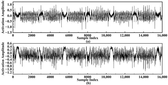
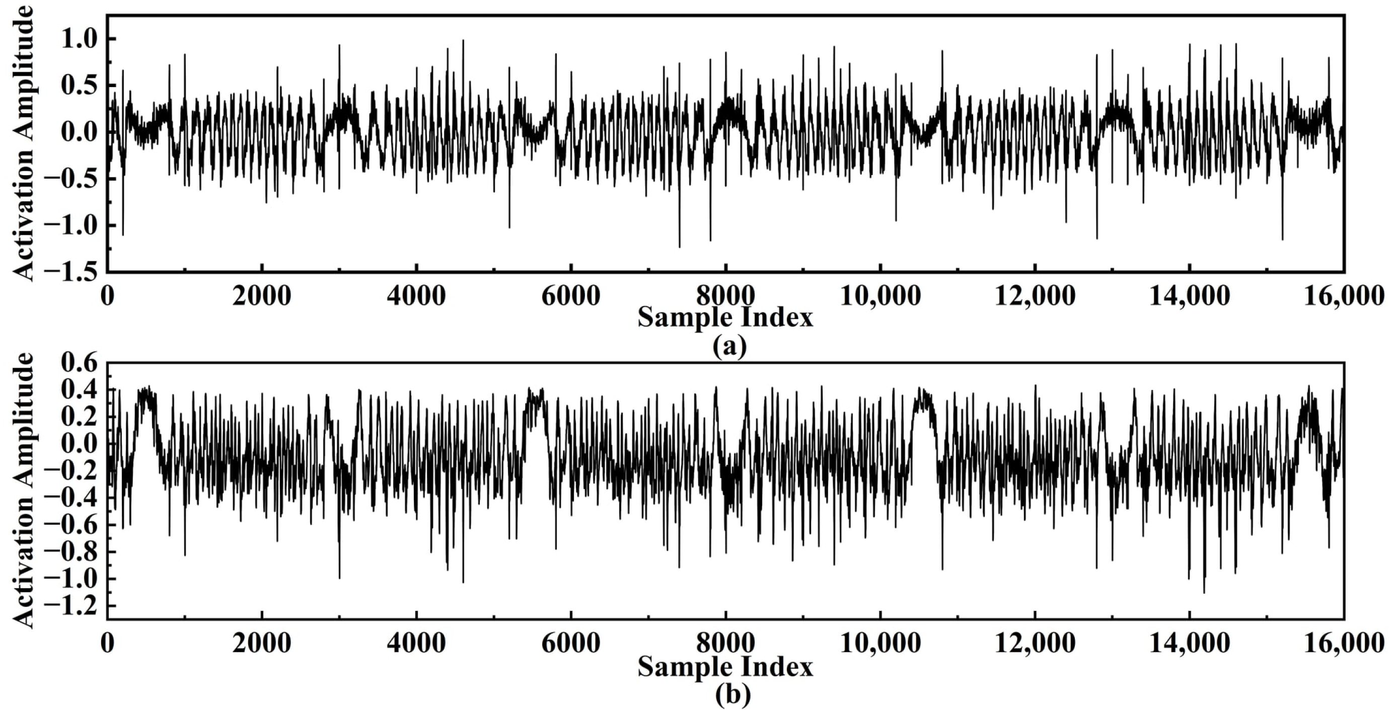
Figure 3 shows the feature maps generated from two convolutional layers of the trained IATWSB-1D-CNN shown in Figure 2a. Figure 3a shows the feature activations from the first convolutional layer, and Figure 3b shows the feature activations from the second convolutional layer. As shown in Figure 3a, the first convolutional layer responds primarily to low-level local temporal features within SMI signals, such as fringe edges and amplitude fluctuations. As features propagate to the second convolutional layer, more abstract displacement-related temporal components are highlighted in Figure 3b. The results indicate that displacement-related features are progressively extracted from shallow to deep layers and enable the network to effectively learn displacement-related local features.
Figure 3.
Feature activations from the two convolutional layers: (a) the first convolutional layer; (b) the second convolutional layer.
2.3. Simulation of SMI Signals
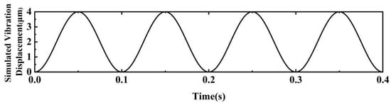
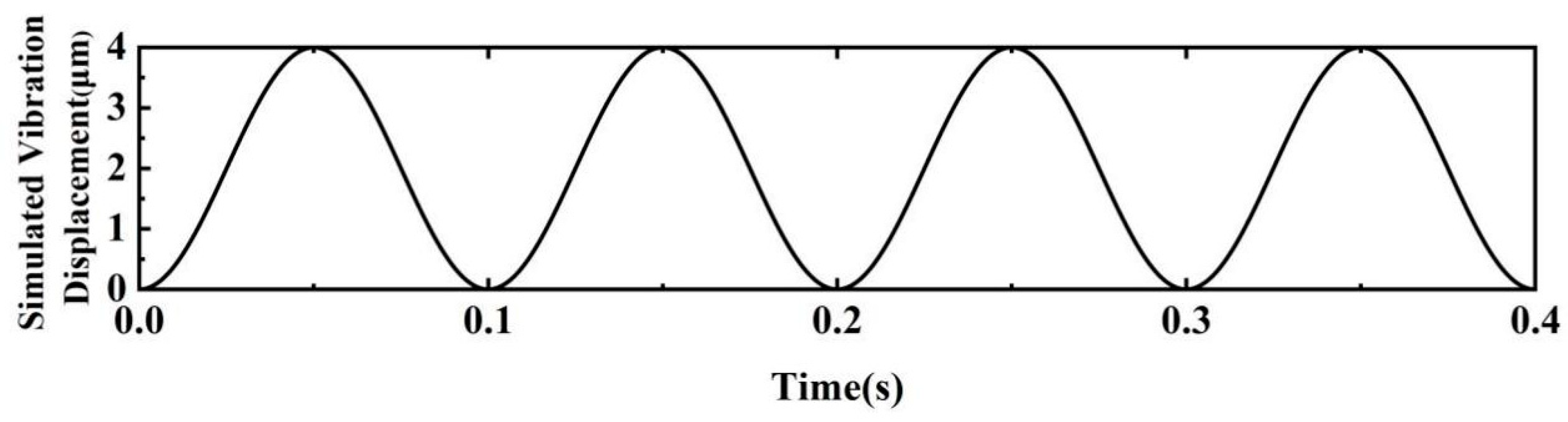
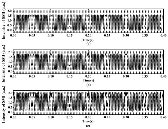
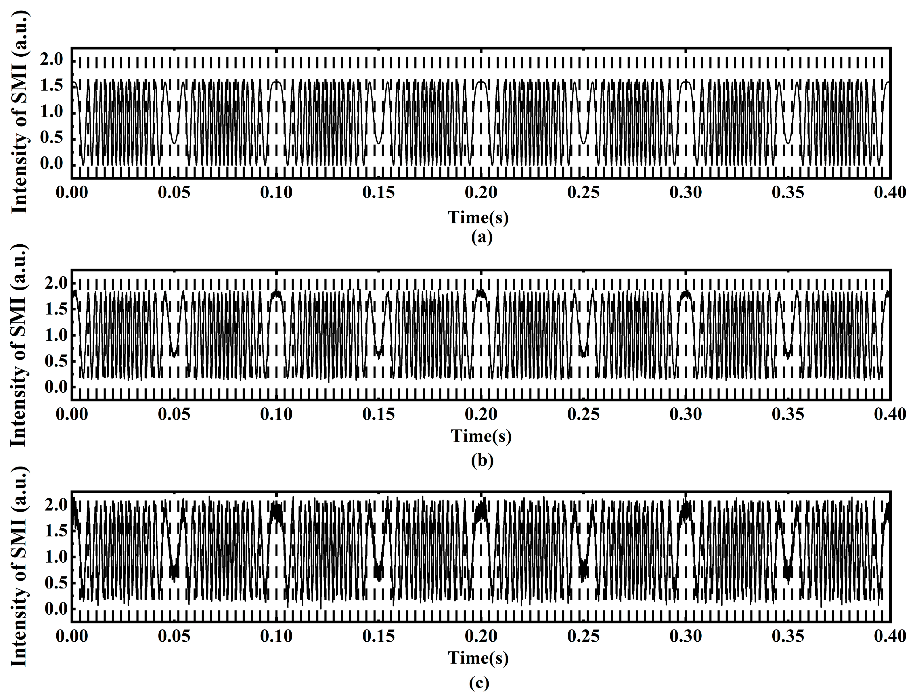
Figure 4 shows the simulated vibration displacement of the object, which varies sinusoidally with the amplitude of 2 μm and the period of 0.1 s. Figure 5 shows the time-window segmented simulation SMI signals at different levels of signal-to-noise ratios (SNRs) with the Lang–Kobayashi (L-K) model [31]. The simulated SMI signals are segmented into 100 consecutive local signal sequences using a window length of 200 sampling points, which is consistent with the window length used in previous work [23]. The per-window predicted displacements are assembled chronologically, remaining continuous across boundaries owing to the adjacent, non-overlapping windows. All signal sequences are divided chronologically into two subsets, with the first 80% used for training and the remaining 20% reserved for testing. The test set is not used during training. Figure 5a exhibits the simulated SMI signals based on the simulation parameters shown in Table 2. Figure 5b and Figure 5c show the simulated SMI signals at SNRs of 30 dB and 20 dB, respectively.
Figure 4.
Simulated vibration displacement of the object.
Figure 5.
Time-window segmented simulation SMI signals with different levels of SNRs. (a) Clean signal; (b) 30 dB; (c) 20 dB.
Table 2.
Parameters used in the simulation.
2.4. Comparison of Displacement Reconstruction for the Simulated SMI Signals
To demonstrate the performance of the displacement reconstruction, a comparison of the displacement reconstructed by the IATWSB-1D-CNN method and the phase unwrapping method is conducted. To quantitatively evaluate the deviation between the reconstructed and simulated displacement, the RMSE is introduced as the evaluation parameter. The RMSE with the IATWSB-1D-CNN is calculated on the test set, which is not used during network training. The phase unwrapping method is a deterministic, training-free algorithm that learns no parameters from the data and requires no training set. The reconstruction error is evaluated over the same test set as those used for the IATWSB-1D-CNN method. The RMSE between the normalized reconstructed displacement curve and the normalized simulated displacement curve is calculated by Equation (1) [32], in which each curve is normalized by dividing by the peak-to-peak displacement, so that the normalized curves fall within the range [0, 1]. The physical RMSE can be recovered by multiplying the normalized RMSE by the peak-to-peak displacement.
where Hi is the reconstructed normalized displacement of the i-th sampling point; yi is the normalized nominal displacement of the i-th sampling point; and N is the total number of sampling points.
The ablation experiments are conducted in simulated SMI signals by removing Batch Normalization and Dropout layers individually, while keeping the remaining network configurations and the data segmentation unchanged. The reconstruction accuracy is evaluated with the same test set under noise-free conditions and at SNRs of 30 dB and 20 dB using the normalized RMSE. The results are summarized in Table 3.
Table 3.
Results of the ablation experiments using the IATWSB-1D-CNN in simulated SMI signals under noise-free, 30 dB, and 20 dB conditions.
As shown in Table 3, the IATWSB-1D-CNN with both Batch Normalization and Dropout achieves the lowest reconstruction error. The RMSE values are 0.032, 0.060, and 0.100 under the noise-free condition and at SNRs of 30 dB and 20 dB, respectively. The RMSE increases to 0.046, 0.076, and 0.287 after removing the Batch Normalization layer under the three conditions, respectively. The RMSE raises to 0.058, 0.191, and 0.398 after removing the Dropout layer, respectively, with notably larger degradation at 30 dB and 20 dB. These results demonstrate that both the Batch Normalization and Dropout layers contribute to the reconstruction accuracy with the IATWSB-1D-CNN method.
The SMI signals shown in Figure 5 are used for displacement reconstruction under the noise-free condition and SNRs of 30 dB and 20 dB, respectively. For each condition, the displacement is reconstructed using the IATWSB-1D-CNN method and the phase unwrapping method [33], and the comparison results are shown in Figure 6 and Figure 7.
Figure 6.
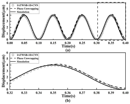
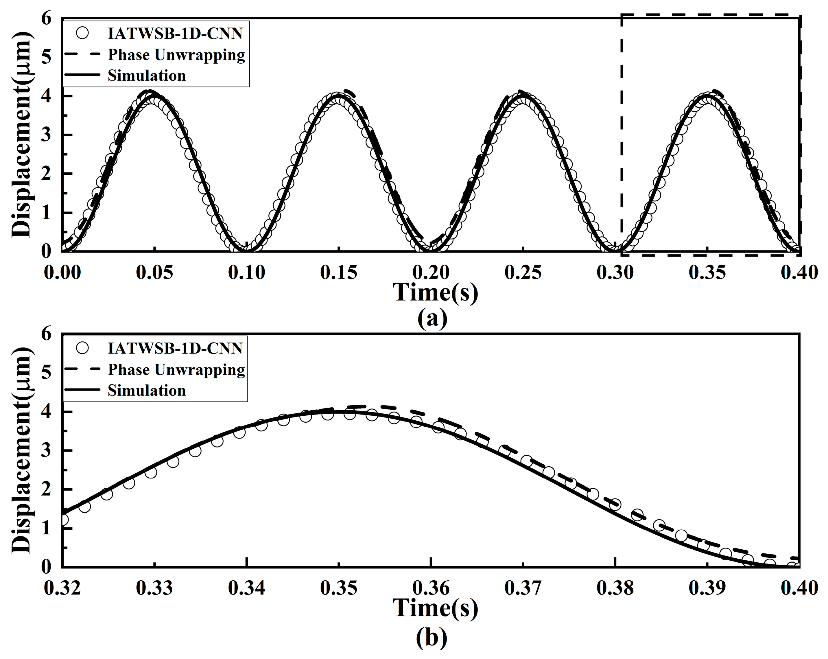
Comparison of displacement reconstruction results without noise. (a) Full view of the comparison; (b) magnified view of the evaluation segment marked by the dotted rectangle line.
Figure 7.
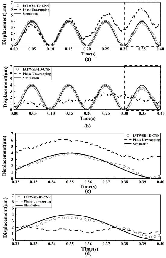
Comparison of displacement reconstruction results under SNRs of 30 dB and 20 dB: (a) 30 dB; (b) 20 dB; (c) magnified view of the evaluation segment marked by the dotted rectangle line in (a); (d) magnified view of the evaluation segment marked by the dotted rectangle line in (b).
Figure 6 shows the displacement reconstruction results obtained by the IATWSB-1D-CNN method and the phase unwrapping method with noise-free data. The solid curve represents the simulated vibration displacement, which is used as the reference displacement. The circles denote the displacement obtained by the IATWSB-1D-CNN method, while the dashed curve represents the displacement reconstructed using the phase unwrapping method.
As can be seen from Figure 6a, the displacement curves reconstructed by the IATWSB-1D-CNN method and the phase unwrapping method closely overlap with the simulated vibration displacement curve. The enlarged evaluation segment view shown in Figure 6b demonstrates that the displacement curves reconstructed by the IATWSB-1D-CNN and the phase unwrapping method maintain excellent consistency with the simulated vibration displacement curve. The RMSE values of the IATWSB-1D-CNN and phase unwrapping methods under noise-free conditions are 0.032 and 0.049, respectively. The results demonstrate that both methods are capable of completing displacement reconstruction under noise-free conditions, and the IATWSB-1D-CNN achieves higher reconstruction accuracy.
Figure 7 presents the reconstructed displacement obtained by the IATWSB-1D-CNN method and the phase unwrapping method under noisy conditions, where Figure 7a,c correspond to the results at the SNR of 30 dB, and Figure 7b,d correspond to the results at the SNR of 20 dB. Figure 7c,d show the magnified views of the evaluation segment.
As shown in Figure 7a at an SNR of 30 dB, the reconstruction curve of the phase unwrapping method exhibits more prominent deviations within the period of 0.2 s to 0.4 s than those within the period of 0.0 s to 0.2 s, while the displacement reconstructed using the IATWSB-1D-CNN method remains highly consistent with the simulated vibration displacement. Figure 7c presents the magnified view of the evaluation segment at 30 dB. Within this segment, the displacement reconstructed by the IATWSB-1D-CNN method nearly overlaps with the simulated vibration displacement, whereas the displacement reconstructed by the phase unwrapping method exhibits an evident deviation. The RMSE values corresponding to the IATWSB-1D-CNN and phase unwrapping methods are 0.060 and 0.59, respectively. As illustrated in Figure 7b, at the lower SNR of 20 dB, the displacement reconstruction by the phase unwrapping method failed. Although the displacement reconstruction by the IATWSB-1D-CNN method is also affected by noise during the 0.2–0.4 s interval, it remains highly consistent with the simulated vibration displacement. Figure 7d presents the magnified view of the evaluation segment at 20 dB. Within this segment, the displacement reconstructed by the phase unwrapping method deviates substantially from the simulated vibration displacement, whereas the displacement reconstructed by the IATWSB-1D-CNN closely follows the reference displacement despite the presence of noise. The RMSE values corresponding to the IATWSB-1D-CNN and phase unwrapping methods are 0.100 and 0.63, respectively. Based on the results from Figure 6 and Figure 7, it can be concluded that the IATWSB-1D-CNN method exhibits stronger anti-noise capability in micro-displacement reconstruction than the phase unwrapping method.
Table 4 summarizes the reconstruction accuracy expressed in physical metrological units. The normalized RMSE is converted into the physical RMSE (nm) by multiplying it by the peak-to-peak displacement. The physical RMSE is then expressed as a ratio relative to the half-wavelength fringe resolution (λ/2 ≈ 317.5 nm), where a value below unity indicates sub-fringe accuracy.
Table 4.
Conversion of normalized RMSE to physical RMSE and comparison with the half-wavelength resolution under three conditions.
As shown in Table 4, the physical RMSE values using the IATWSB-1D-CNN method under the noise-free condition, at the SNRs of 30 dB and 20 dB are 128 nm, 240 nm, and 400 nm, corresponding to 0.40, 0.76, and 1.26 times λ/2, respectively. The sub-fringe reconstruction accuracy can be obtained by the IATWSB-1D-CNN method under the noise-free and 30 dB conditions, while slightly higher than the fringe resolution at 20 dB. These results indicate that the better reconstruction accuracy and stronger anti-noise capacity can be maintained by the IATWSB-1D-CNN.
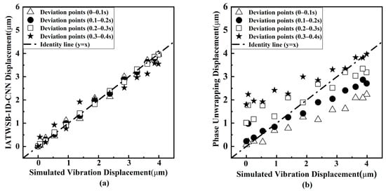
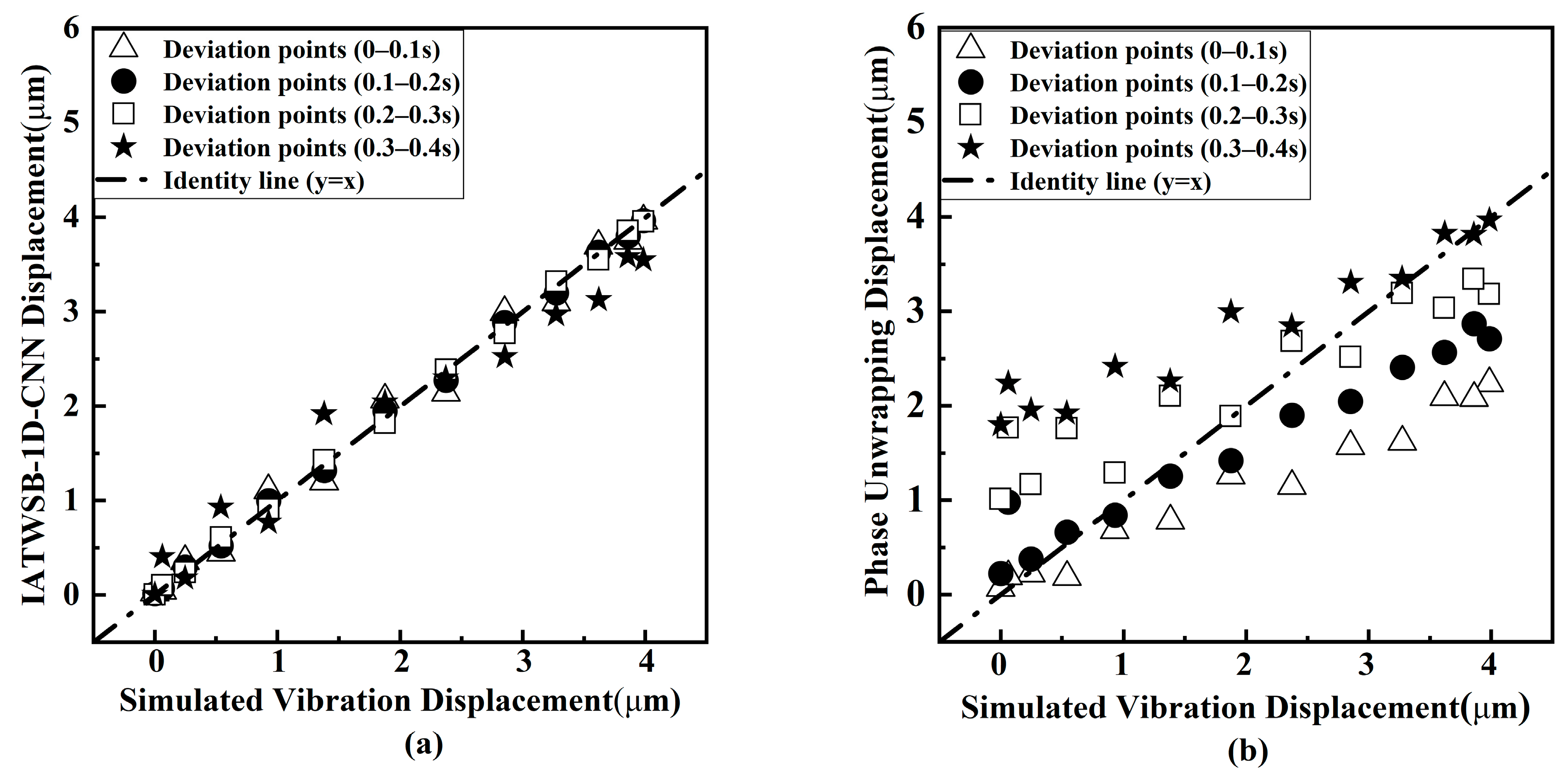
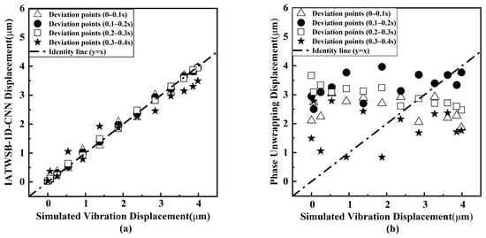
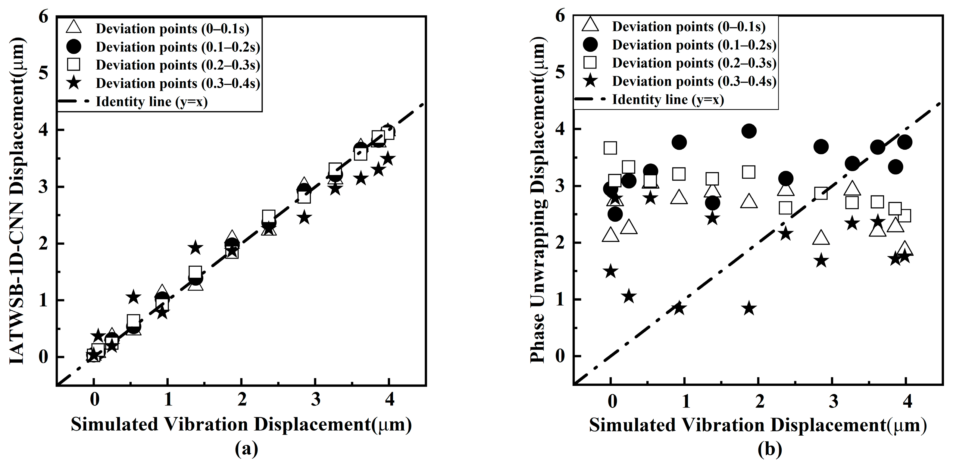
To compare the stability and anti-noise capability of the displacement reconstruction by the IATWSB-1D-CNN and the phase unwrapping method, the scatter diagrams and per-cycle RMSE curves are presented. Figure 8, Figure 9 and Figure 10 present the cycle-wise scatter diagrams of the reconstructed displacement against the simulated vibration displacement under the noise-free condition and SNRs of 30 dB and 20 dB, respectively. In the figures, the four vibration cycles, corresponding to the time ranges of 0–0.1 s, 0.1–0.2 s, 0.2–0.3 s, and 0.3–0.4 s, are marked by the different marker shapes. The dashed–dotted line represents the identity line (y = x), corresponding to a one-to-one relationship between the reconstructed and simulated vibration displacements. The closer the scatter points are to this line, the better the consistency between the reconstructed and simulated displacement. For the IATWSB-1D-CNN method in Figure 8, Figure 9 and Figure 10, the time range of the training data is from 0 to 0.3s, which corresponds to the first three vibration cycles; for the fourth cycle with the time range from 0.3 to 0.4s, the training data is contained in the time range from 0.3 to 0.32s and the test data is contained from 0.32 to 0.4s.
Figure 8.
Cycle-wise scatter diagrams of displacement reconstruction results under noise-free conditions. (a) IATWSB-1D-CNN method; (b) phase unwrapping method.
Figure 9.
Cycle-wise scatter diagrams of displacement reconstruction results at an SNR of 30 dB. (a) IATWSB-1D-CNN method; (b) phase unwrapping method.
Figure 10.
Cycle-wise scatter diagrams of displacement reconstruction results at an SNR of 20 dB. (a) IATWSB-1D-CNN method; (b) phase unwrapping method.
Figure 8 shows the cycle-by-cycle scatter diagrams of the displacement reconstruction results under noise-free conditions. Figure 8a presents the results obtained by the IATWSB-1D-CNN method, while Figure 8b presents those obtained by the phase unwrapping method. As shown in Figure 8a, the scatter points obtained by the IATWSB-1D-CNN method are generally distributed close to the identity line throughout the four cycles. Although the scatter points obtained by the phase unwrapping method in Figure 8b are also generally distributed around the identity line, the scatter points obtained by the IATWSB-1D-CNN method are more closely concentrated around the identity line than those obtained by the phase unwrapping method.
Figure 9 shows the cycle-by-cycle scatter diagrams of the displacement reconstruction results at an SNR of 30 dB. As shown in Figure 9a, the scatter points obtained by the IATWSB-1D-CNN method remain generally concentrated around the identity line, although slight dispersion can be observed in the fourth cycle (0.3 s–0.4 s) due to the influence of noise. In contrast, the scatter points obtained by the phase unwrapping method in Figure 9b become more deviated than those under noise-free conditions, progressively deviating further from the identity line as the vibration cycle index increases.
Figure 10 shows the cycle-by-cycle scatter diagrams of the displacement reconstruction results at an SNR of 20 dB. Compared with the results at the SNR of 30 dB, the difference in the scatter-point distributions between the two methods becomes clearer. The scatter points obtained by the IATWSB-1D-CNN method in Figure 10a are also affected by the increased noise level, but they remain generally distributed around the identity line. Moreover, the degree of dispersion remains relatively consistent across the four cycles. As shown in Figure 10b, the scatter points obtained by the phase unwrapping method are randomly and irregularly distributed across the four cycles, with considerable deviations from the identity line and several points exhibiting clear discrepancies.
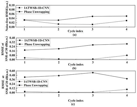
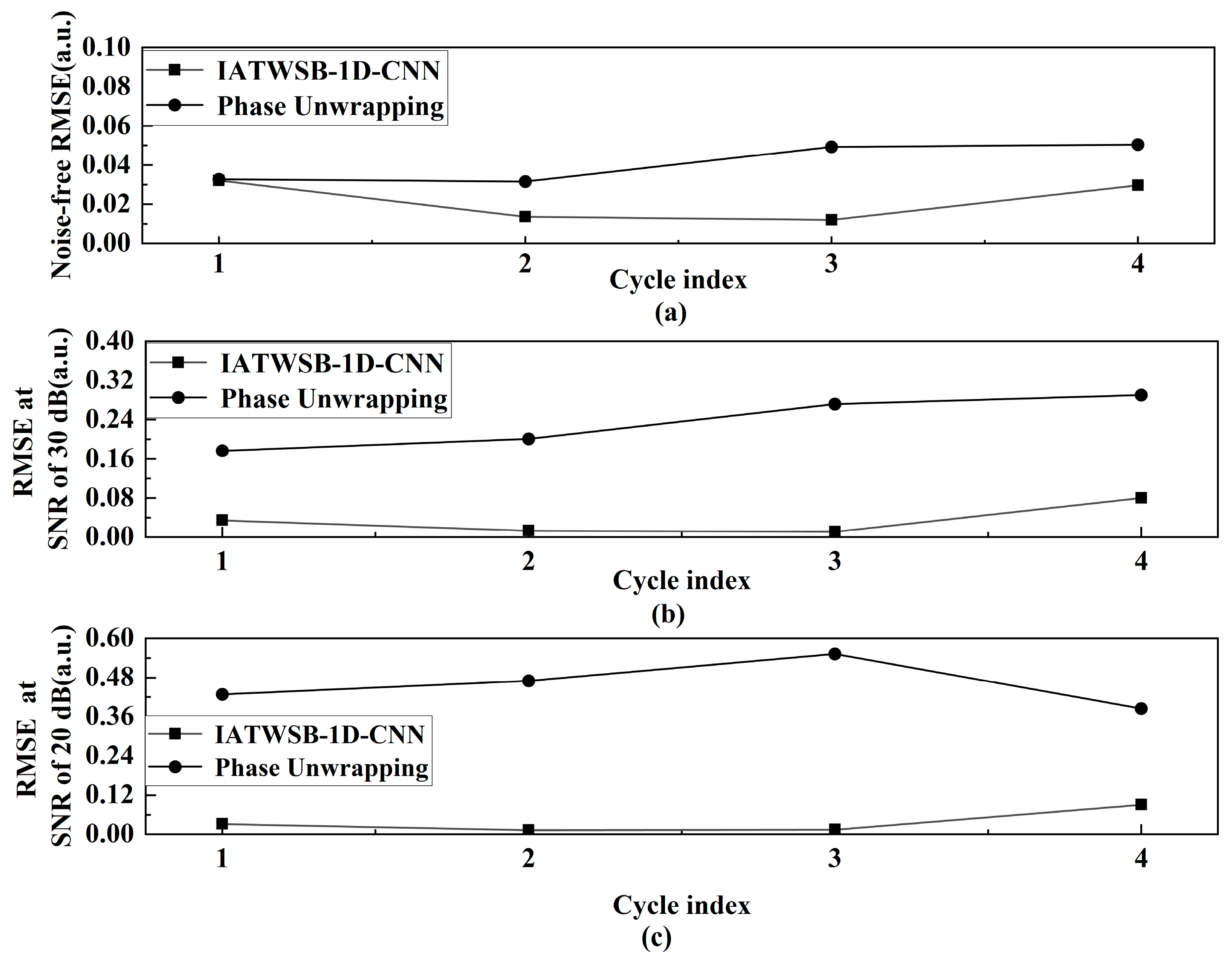
The RMSE values of the IATWSB-1D-CNN method and the phase unwrapping method are quantitatively compared for each cycle. The RMSE is calculated through Equation (1). Figure 11 presents the evolution of the RMSE across the four cycles. Figure 11a–c correspond to the noise-free condition and SNRs of 30 dB and 20 dB, respectively. For the IATWSB-1D-CNN method in Figure 11, the per-cycle comparison in cycles 1–3 reflects fitting on training data, while both the training data (0.3–0.32 s) and the test data (0.32–0.4 s) are contained in cycle 4.
Figure 11.
The RMSE variation curves of each cycle: (a) noise-free; (b) 30 dB; (c) 20 dB. (Cycle indices 1, 2, 3, and 4 represent the time ranges of 0–0.1 s, 0.1–0.2 s, 0.2–0.3 s, and 0.3–0.4 s, respectively.).
As can be seen from Figure 11a, the RMSE of the IATWSB-1D-CNN remains roughly within the range from 0.01 to 0.03, whereas the RMSE of the phase unwrapping method exhibits higher fluctuations approximately between 0.03 and 0.05. Moreover, the RMSE of the phase unwrapping method shows a slight upward trend across the four time ranges. These results show that the reconstructed displacement obtained using both methods performs well under noise-free conditions, which is consistent with the qualitative observation from Figure 8.
As shown in Figure 11b at the SNR of 30 dB, the RMSE values of the IATWSB-1D-CNN method remain stable over the four time ranges; the RMSE of the phase unwrapping method exhibits an increasing trend across successive cycles. The results in Figure 7a and Figure 11b both demonstrate that the IATWSB-1D-CNN method maintains accurate and stable displacement reconstruction, while the phase unwrapping method exhibits the accumulation of errors during reconstruction.
When the SNR is reduced to 20 dB, as shown in Figure 11c, the RMSE of the IATWSB-1D-CNN method remains relatively stable across all four time ranges. In contrast, the RMSE of the phase unwrapping method exceeds 0.36 and remains considerably higher than that of the IATWSB-1D-CNN method. This trend is consistent with the observation in Figure 7b.
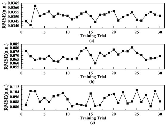
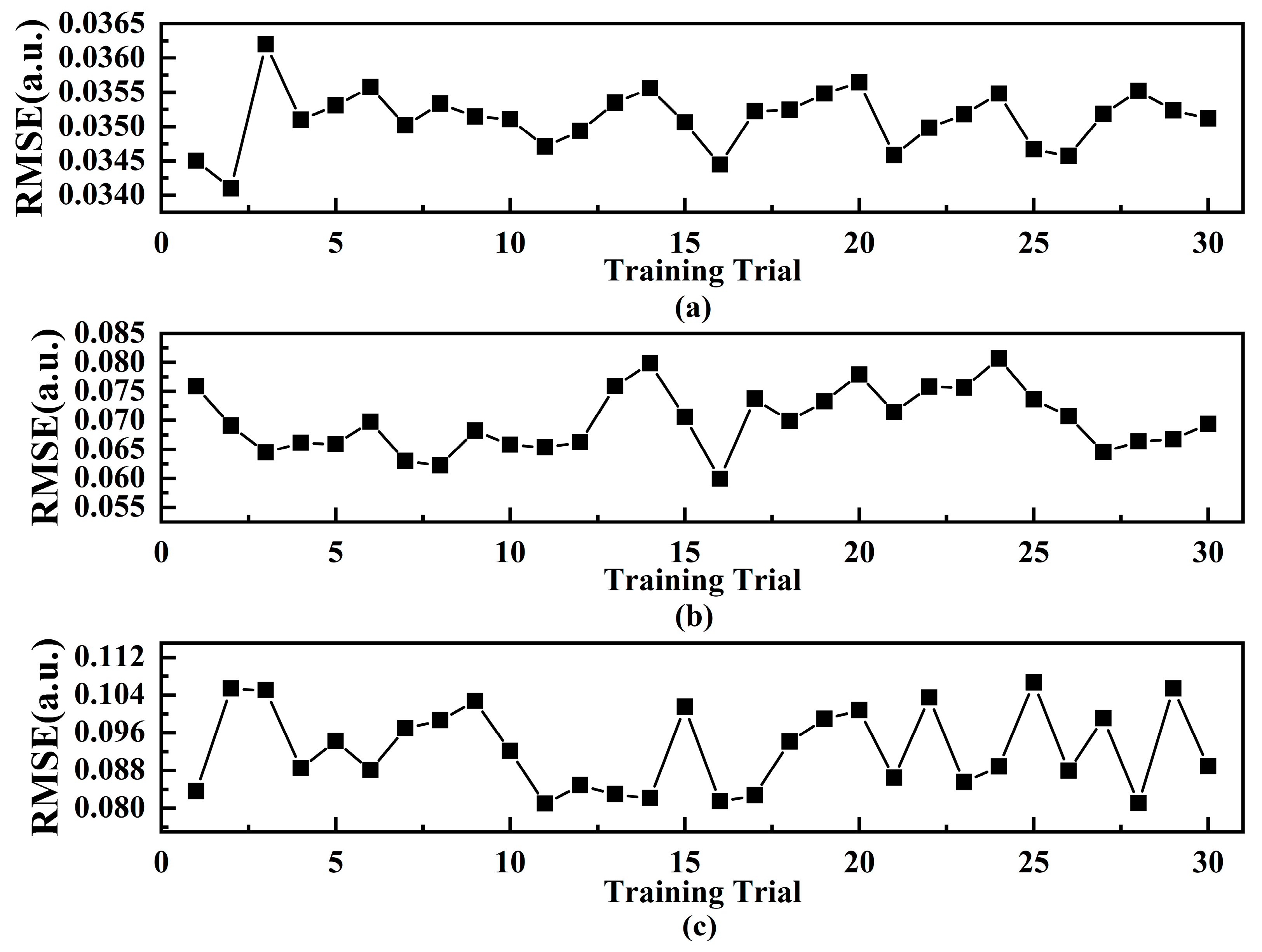
To evaluate the stability and reproducibility of the IATWSB-1D-CNN across repeated training, the network is independently trained 30 times using identical datasets and network architecture under the noise-free condition and SNRs of 30 dB and 20 dB, respectively. All 30 independent training are adopted with the same dataset splitting strategy as described above. Figure 12 presents the calculated RMSE values based on the test set over the 30 training trials under the three conditions.
Figure 12.
Calculated RMSE values based on the IATWSB-1D-CNN method over 30 training trials: (a) noise-free; (b) 30 dB; (c) 20 dB.
As shown in Figure 12a, the RMSE of the IATWSB-1D-CNN method locals between 0.034 and 0.037 across the 30 training trials under the noise-free condition. As shown in Figure 12b, the RMSE distributes approximately between 0.060 and 0.081 at the SNR of 30 dB. When the SNR is reduced to 20 dB as shown in Figure 12c, the RMSE ranges approximately from 0.080 to 0.106. Across all three conditions, the RMSE values remain within relatively consistent ranges over repeated training. These results indicate that the reconstructed displacement of the IATWSB-1D-CNN method remains stable across repeated training under all three conditions.
To quantitatively evaluate the dispersion of the RMSE values over the 30 training trials, the SD and the CV are calculated by Equations (2) and (3), respectively [34]:
where n (here n = 30) is the total number of training trials, j is the index of the training trial, xj denotes the RMSE obtained from the j-th training trial, and is the mean RMSE of the 30 training trials.
where SD is the standard deviation calculated by Equation (2), and is the mean RMSE of the 30 training trials.
The RMSE values (mean ± SD) for 30 independent trainings are 0.0350 ± 0.0004, 0.0701 ± 0.0054, and 0.0926 ± 0.0087 under noise-free conditions and at SNRs of 30 dB and 20 dB, respectively. The corresponding CVs are 1.2%, 7.7%, and 9.4% respectively. All CV values are below the 10% threshold for acceptable repeatability, indicating relatively low variability across the repeated training trials [28]. These results demonstrate that the IATWSB-1D-CNN method achieves stable and reproducible displacement reconstruction across repeated training.
3. Experiment Design and Implementation
3.1. Experimental Setup
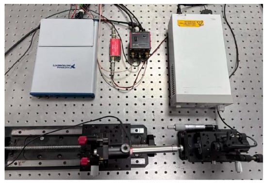
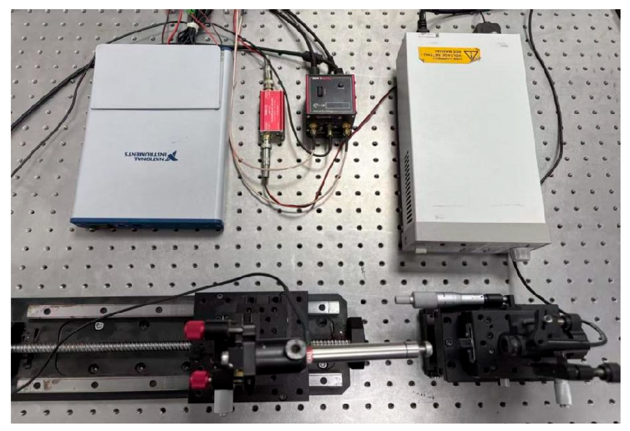
The experimental setup is illustrated in Figure 13. The experimental system mainly consists of a semiconductor laser, a PZT-based displacement actuator, a mechanical translation stage for external-cavity adjustment, and a signal acquisition card. A 635 nm semiconductor laser is employed to establish the SMI optical path, with the PZT serving as the moving target. The PZT-based displacement actuator is driven by a piezoelectric controller (Thorlabs KPZ101) to generate the prescribed micro-displacement. In this experiment, the absolute displacement of the PZT-based actuator cannot be directly feedbacked. The vibration amplitude of a piezoelectric ceramic is proportional to its driving voltage [35]. The reference displacement is therefore represented by the normalized PZT modulation voltage. The error resulting from the nonlinear reaction of the PZT and the surrounding mechanical disturbance is on the order of λ/200 and can be ignored relative to the displacement amplitude. Accordingly, it is appropriate to use the normalized PZT modulation voltage as the reference for evaluating reconstruction accuracy [36]. The laser operating current is regulated by a laser diode controller (Thorlabs LDC205C), while the external cavity length is adjusted by a mechanical translation stage and maintained at 85.14 mm throughout the measurements. The optical feedback-induced SMI signal is then converted into a voltage signal and amplified by a current-to-voltage conversion circuit. The processed signal is sampled by the signal acquisition card (NI USB-6341) and transmitted to a computer for waveform monitoring and subsequent displacement reconstruction.
Figure 13.
Experimental setup for laser self-mixing interferometry.
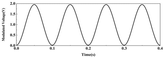
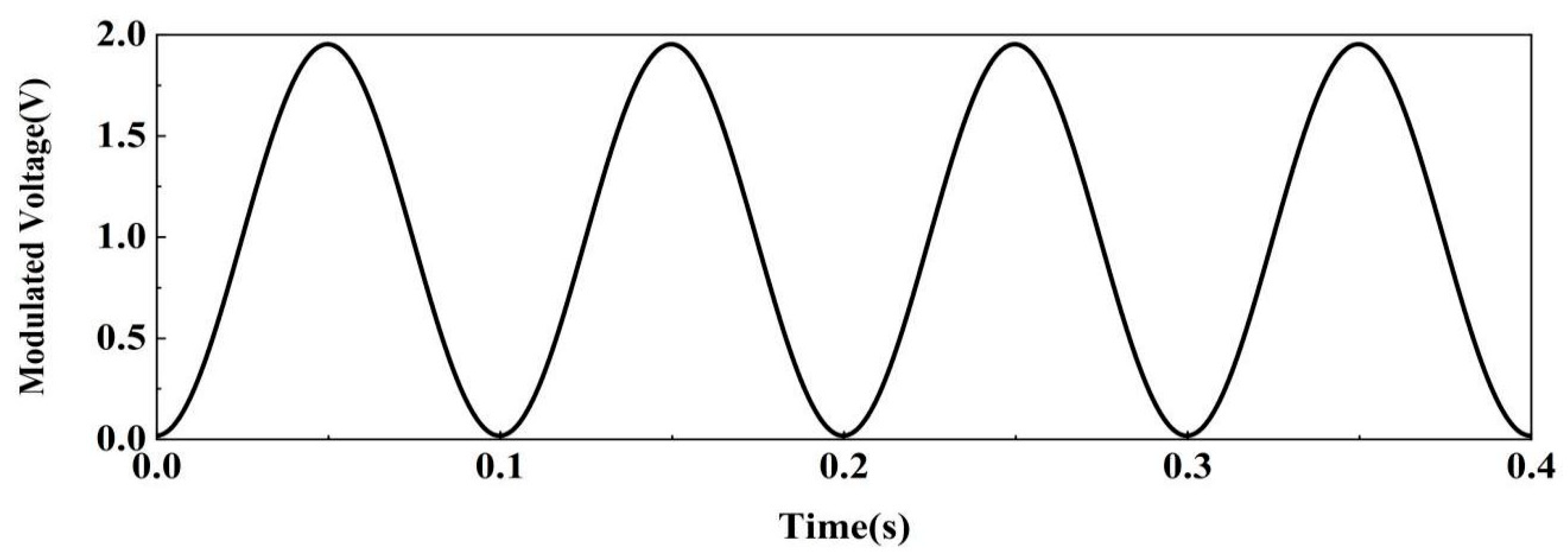
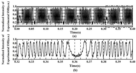
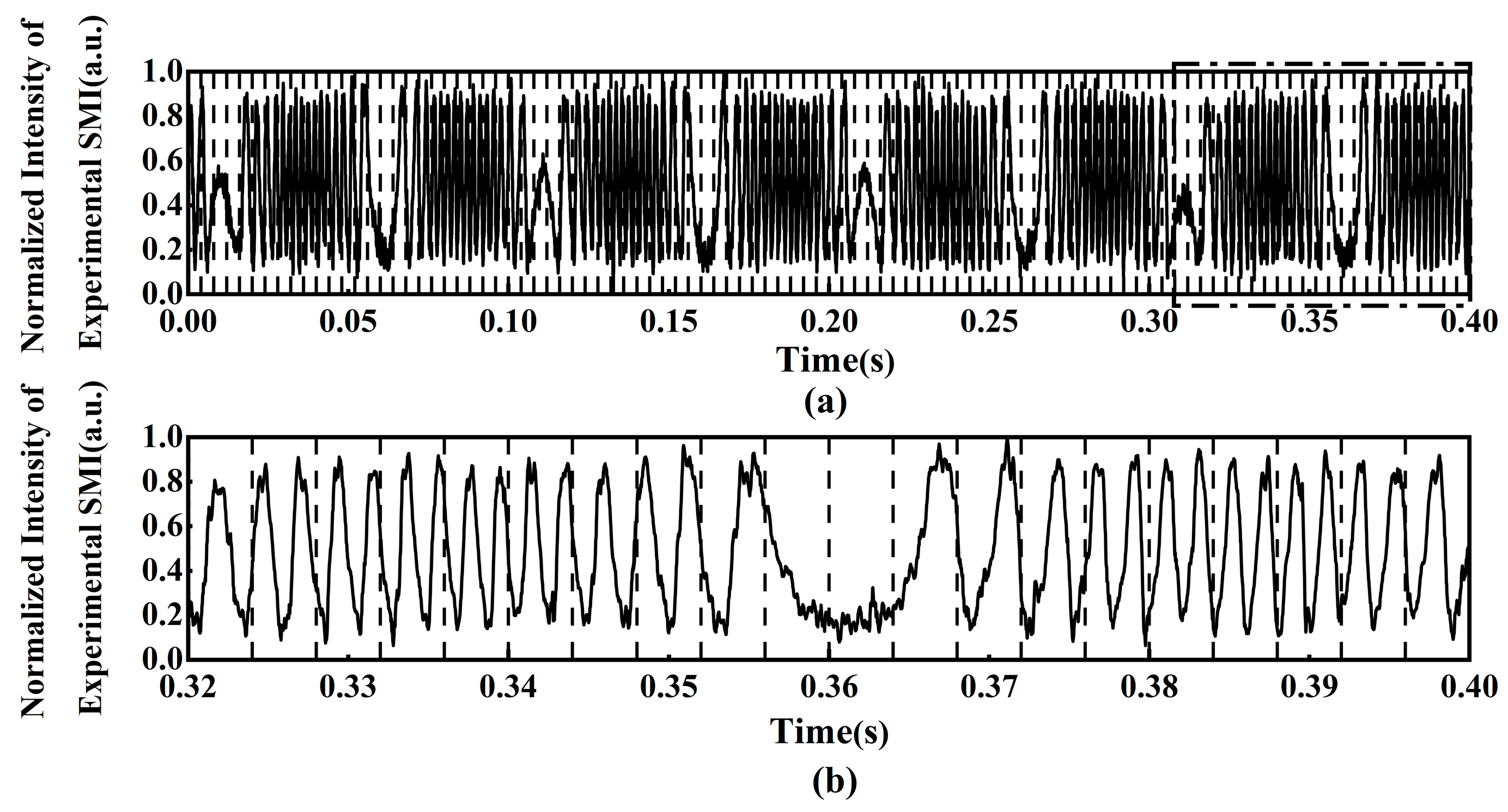
Figure 14 shows the curve of the PZT modulation voltage; the time-window segmented normalized experimental SMI signals are shown in Figure 15. As shown in Figure 15a, the black dotted lines indicate the segmentation boundaries of each local signal sequence. The experimental SMI signals are segmented into 100 consecutive local signal sequences using a window length of 200 sampling points, with 80% used for training and 20% for testing. As shown in Figure 15b, the enlarged view of the region marked by the dotted rectangle in Figure 15a presents the test set of the segmented experimental SMI signals.
Figure 14.
Curve of PZT modulation voltage.
Figure 15.
Time-window segmented normalized intensity of experimental SMI signals: (a) time-window segmented experimental SMI signals marked by the vertical dotted lines; (b) enlarged view of the segmented experimental SMI signals marked by a dotted rectangle line shown in (a).
3.2. Comparison of Displacement Reconstruction for Experimental SMI Signals
The ablation experiments are conducted with the experimental SMI signals by removing Batch Normalization and Dropout layers individually while keeping all other configurations and data segmentation unchanged. The RMSE with each architecture is evaluated with the same test set, and the results are summarized in Table 5.
Table 5.
The results of the ablation experiments using the IATWSB-1D-CNN in experimental SMI signals.
As shown in Table 5, the lowest RMSE of 0.062 is achieved by the IATWSB-1D-CNN with both Batch Normalization and Dropout layers. The RMSE increases to 0.079 and 0.223 when the Batch Normalization and Dropout layers are removed individually, respectively. These results indicate that both layers improve the reconstruction accuracy and generalization of the network in the experiment.
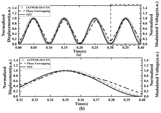
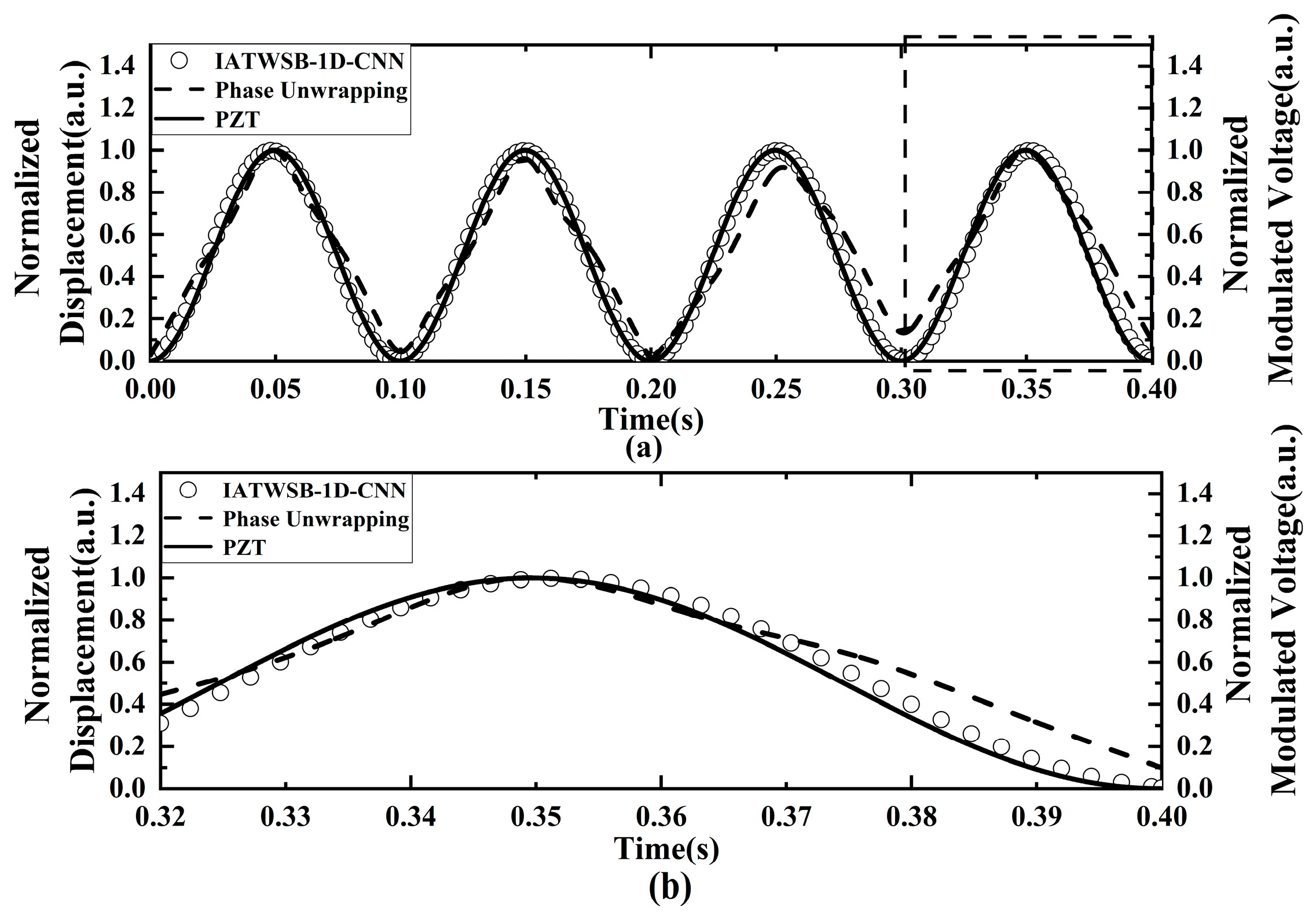
Figure 16 shows the comparison of the normalized PZT modulation voltage and the normalized displacement reconstruction curves. The RMSE is calculated through Equation (1).
Figure 16.
Comparison of normalized PZT modulation voltage (solid line) and the normalized displacement reconstruction curves. (a) Full view of the comparison; (b) magnified view of the evaluation segment marked by the dotted rectangle line.
As can be seen from Figure 16a, the displacement curve predicted by the IATWSB-1D-CNN method closely follows the curve of the normalized modulated voltage over the entire cycle. The displacement reconstructed by the phase unwrapping method generally follows the curve of the normalized modulated voltage, whereas it exhibits clearer deviations than those of the IATWSB-1D-CNN method, particularly around the peaks and troughs. The enlarged evaluation segment view is shown in Figure 16b. The displacement predicted by the IATWSB-1D-CNN method remains in close agreement with the normalized modulated voltage, whereas the displacement reconstruction by the phase unwrapping method exhibits an evident deviation around the peak within the time range of 0.20–0.30 s. The RMSE values corresponding to the IATWSB-1D-CNN and phase unwrapping methods are 0.062 and 0.115, respectively. Owing to the relatively low noise level in the experiment, the difference in RMSE between the two methods is less pronounced than that observed under higher noise levels. These results indicate that the IATWSB-1D-CNN method can achieve more accurate displacement reconstruction in the experiments, while the phase unwrapping method is more susceptible to error accumulation during reconstruction of practical SMI signals.
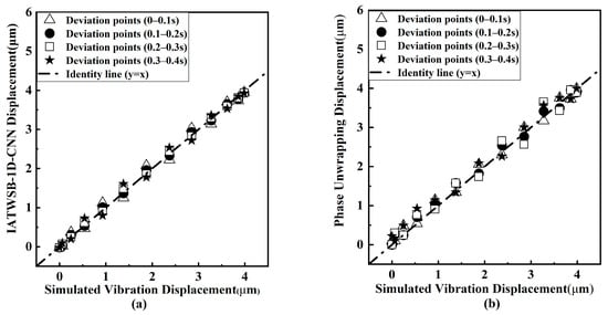
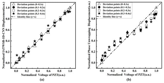
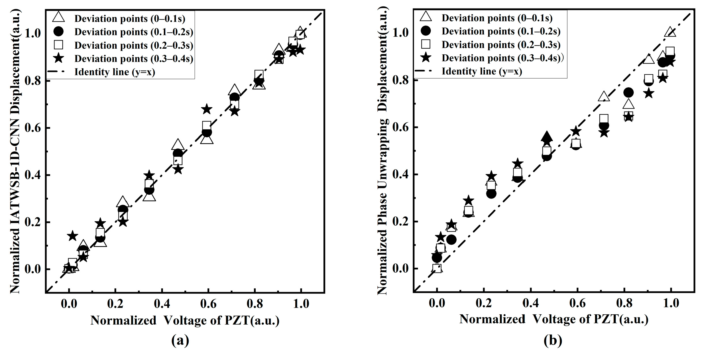
Figure 17 shows the cycle-by-cycle scatter diagrams of the normalized displacement reconstruction results obtained from the experimental SMI signals. For the IATWSB-1D-CNN method in Figure 17, the time range of the training data is from 0 to 0.3s, which corresponds to the first three vibration cycles; for the fourth cycle with the time range from 0.3 to 0.4s, the training data is contained in the time range from 0.3 to 0.32s and the test data is contained from 0.32 to 0.4s. Figure 17a presents the results obtained by the IATWSB-1D-CNN method, while Figure 17b presents those obtained by the phase unwrapping method. As shown in Figure 17a, the scatter points obtained by the IATWSB-1D-CNN method are generally distributed close to the identity line throughout the four cycles, indicating good agreement between the reconstructed displacement and the reference PZT modulation voltage. The scatter points obtained by the phase unwrapping method in Figure 17b exhibit clearer deviations from the identity line than those of the IATWSB-1D-CNN method. The deviation becomes increasingly noticeable as the vibration cycle index increases.
Figure 17.
Cycle-wise scatter diagrams of normalized displacement reconstruction results under experimental conditions: (a) IATWSB-1D-CNN method; (b) phase unwrapping method.
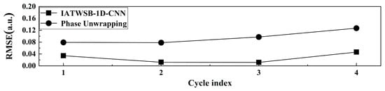
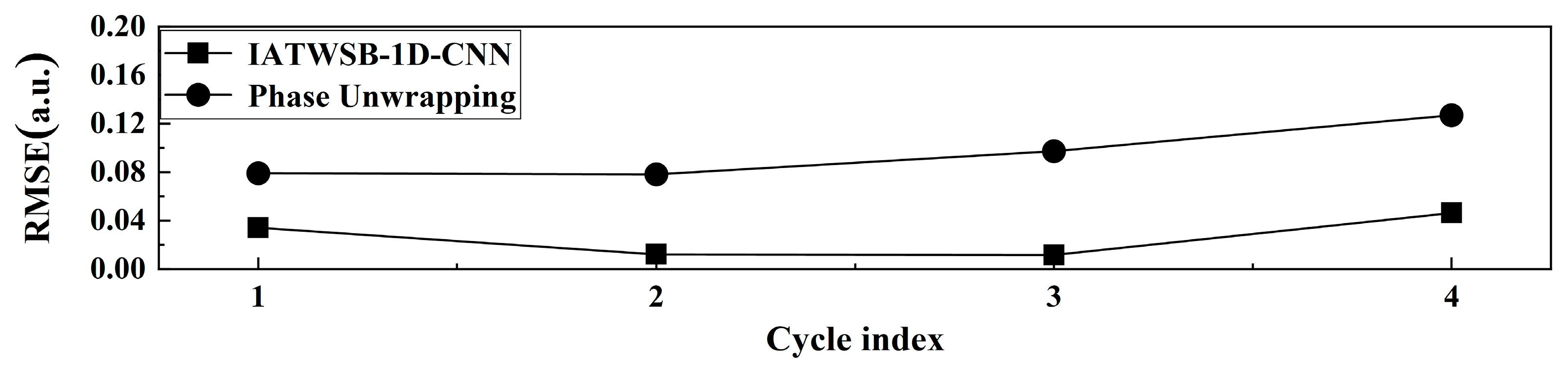
Figure 18 presents the RMSE variation curves of each cycle in the experiment. For the IATWSB-1D-CNN method in Figure 18, the per-cycle comparison in cycles 1–3 reflects fitting on training data, while both the training data (0.3–0.32 s) and the test data (0.32–0.4 s) are contained in cycle 4. The RMSE values shown in Figure 18 using the IATWSB-1D-CNN method (square markers) for the four cycles are 0.034, 0.012, 0.011, and 0.056, respectively; the RMSE values shown in Figure 18 using the phase unwrapping method (circle markers) are 0.078, 0.078, 0.097, and 0.127, respectively. As can be seen from Figure 18, the RMSE values of the phase unwrapping method are consistently higher than those of the IATWSB-1D-CNN method. The results in Figure 18 demonstrate that the displacement reconstruction by the IATWSB-1D-CNN method achieves higher accuracy than that by the phase unwrapping method.
Figure 18.
The RMSE variation curves of each cycle in the experiment. (Cycle indices 1, 2, 3, and 4 represent the time ranges of 0–0.1 s, 0.1–0.2 s, 0.2–0.3 s, and 0.3–0.4 s, respectively.).
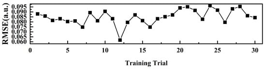
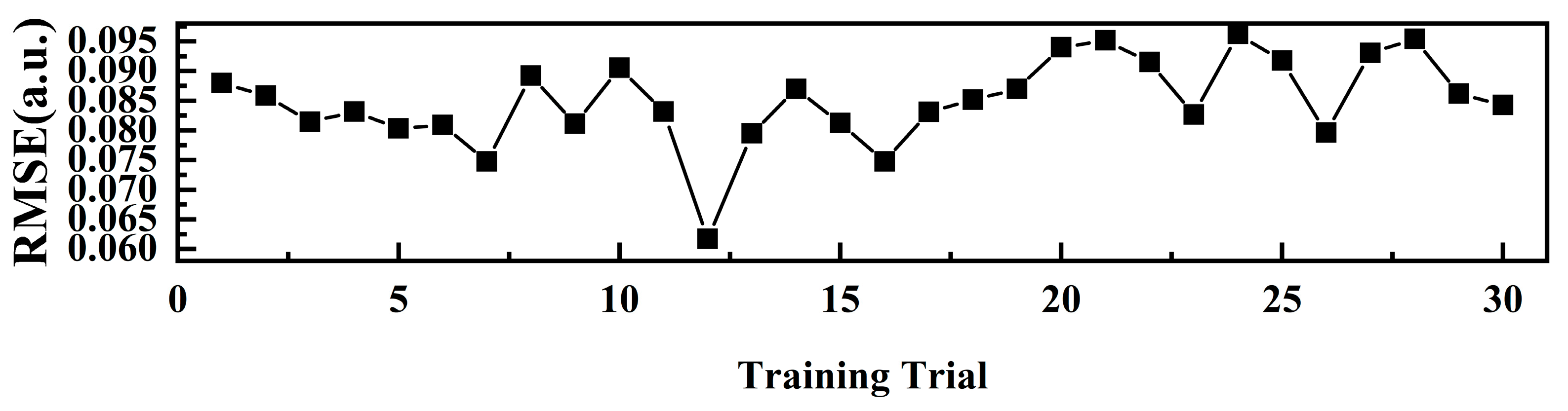
Figure 19 shows the calculated RMSE values based on the IATWSB-1D-CNN method over 30 training trials in the experiment. All 30 independent training runs adopted the same dataset splitting strategy as described above. As shown in Figure 19, the RMSE ranges from approximately 0.060 to 0.095. The RMSE (mean ± SD) is 0.0849 ± 0.0073, corresponding to the CV of 8.6%. The CV is below the 10% threshold for acceptable repeatability [28]. These results demonstrate that the IATWSB-1D-CNN method achieves stable and reproducible displacement reconstruction across repeated training.
Figure 19.
Calculated RMSE values based on the IATWSB-1D-CNN method over 30 training trials in the experiment.
4. Discussion
The results demonstrate that the proposed IATWSB-1D-CNN achieves accurate, anti-noise capability, and reproducible micro-displacement reconstruction in SMI.
First, the ablation results show that the RMSE increases after removing either the Batch Normalization layers or the Dropout layer, and the largest increase occurs at SNR of 20 dB. These findings suggest that Batch Normalization layers and Dropout contribute to reconstruction performance, particularly under noisy conditions. Batch Normalization layers can help regulate the distribution of intermediate activations, whereas Dropout may reduce overfitting and improve generalization.
Second, in physical units (Table 4), the RMSE values of 128 nm, 240 nm, and 400 nm correspond to 0.40, 0.76, and 1.26 times λ/2. Under noise-free and SNR of 30 dB conditions, the reconstruction error remains below the half-wavelength fringe interval, suggesting that the network achieves sub-fringe displacement reconstruction accuracy under these conditions. At an SNR of 20 dB, the reconstruction error slightly exceeds the fringe resolution, which can be attributed primarily to the increased noise level rather than the limitation of the network architecture.
Third, the comparison of RMSE by the IATWSB-1D-CNN method and the phase unwrapping method reveals that the RMSE obtained by the phase unwrapping method exhibits progressive error accumulation across successive vibration cycles and failed at the lower SNR. Whereas the stable per-cycle RMSE is maintained by the IATWSB-1D-CNN. This can be attributed to the direct nonlinear mapping between the SMI signal and displacement, which avoids incremental phase-tracking steps that are prone to error propagation.
Fourth, the CV values of the 30 independent trainings are 1.2%, 7.7%, and 9.4% for the three simulation conditions, respectively, and 8.6% in the experiment. These CVs are all below the 10% threshold here while the CV is 33.1% by the TWSB-1D-CNN method in reference [23] in the experiment. Compared with the results of the displacement reconstruction by the TWSB-1D-CNN method in reference [23] in the experiment, the results of the displacement reconstruction by the proposed IATWSB-1D-CNN method here is more stable and reproducible for multiple independent repeated training.
5. Conclusions
In this paper, the IATWSB-1D-CNN method is proposed for micro-displacement reconstruction in SMI. The continuous SMI signals are divided into fixed-length samples by the time-window segmentation strategy, which avoids directly feeding long continuous signals into the network and improves training efficiency. The simulation results show that the displacement reconstruction using the IATWSB-1D-CNN method exhibits better accuracy and anti-noise capability compared with that using the phase unwrapping method under both noise-free and noisy conditions. In particular, the accuracy of displacement reconstruction by the IATWSB-1D-CNN method remains stable as the noise level increases, whereas that by the phase unwrapping method exhibits a clear degradation. The stability of the IATWSB-1D-CNN method is further evaluated by independently training the network 30 times under the noise-free condition and SNRs of 30 dB and 20 dB. The RMSE values correspond to CVs of 1.2%, 7.7%, and 9.4%, respectively. Experimental results further show the RMSE values of the IATWSB-1D-CNN and the phase unwrapping methods are 0.062 and 0.115, respectively. In addition, the per-cycle RMSE of the IATWSB-1D-CNN method remains consistently lower than that of the phase unwrapping method. The RMSE values from 30 training trials correspond to the CV of 8.6%. These results demonstrate that the IATWSB-1D-CNN method exhibits good performance in reconstruction accuracy, efficiency and anti-noise capability, while maintaining stable and reproducible displacement reconstruction. Furthermore, if the displacement reconstruction in SMI signals with arbitrary waveform is further investigated, the training set for SMI signals with a different frequency or amplitude should be considered.
Author Contributions
Conceptualization, H.L. and Y.Y.; methodology, H.L. and Y.Y.; validation, S.Q. and Y.L.; data curation, Y.Y.; writing—original draft preparation, Y.Y.; writing—review and editing, H.L., Y.Y. and J.S.; supervision, J.S., M.Q. and D.H. All authors have read and agreed to the published version of the manuscript.
Funding
This research was funded by the project supported by the Natural Science Basic Research Plan in Shaanxi Province of China (grant number: 2025JC-YBMS-770), Shaanxi Provincial Innovation Talent Promotion Program—Young Science and Technology Nova Project (grant number: 2026RC-KJXX-147) and Xi’an Young and Middle-aged Leading Scientific and Technological Innovation Talent Project (grant number: 25ZQRC00015).
Institutional Review Board Statement
Not applicable.
Informed Consent Statement
Not applicable.
Data Availability Statement
The data underlying the results presented in this paper are not publicly available at this time but may be obtained from the authors upon reasonable request.
Conflicts of Interest
Dong Hou is employed by the company Focuslight Technologies Inc., and declares no commercial interests. Other authors declare no conflicts of interest.
References
- Acket, G.; Lenstra, D.; Den Boef, A.; Verbeek, B. The influence of feedback intensity on longitudinal mode properties and optical noise in index-guided semiconductor lasers. IEEE J. Quantum Electron. 1984, 20, 1163–1169. [Google Scholar] [CrossRef] [Scilit]
- Donati, S. Developing self-mixing interferometry for instrumentation and measurements. Laser Photonics Rev. 2012, 6, 393–417. [Google Scholar] [CrossRef] [Scilit]
- Taimre, T.; Nikolić, M.; Bertling, K.; Lim, Y.L.; Bosch, T.; Rakić, A.D. Laser feedback interferometry: A tutorial on the self-mixing effect for coherent sensing. Adv. Opt. Photonics 2015, 7, 570–631. [Google Scholar] [CrossRef] [Scilit]
- Han, Y.X.; Cong, Z.C.; Gao, B.K.; Cui, X.Y. Displacement measurement experiment based on laser self-mixing interference frequency modulation signal. Laser Infrared 2022, 52, 695–699. [Google Scholar] [CrossRef]
- Yang, Y.; Li, X.-F.; Kou, K.; Wang, C. Application of All-Phase Spectral Analysis to Self-Mixing Interferometry for Displacement Measurement. Opt. Precis. Eng. 2012, 20, 1740–1746. [Google Scholar] [CrossRef] [Scilit]
- Wang, X.; Zhong, Z.; Chen, H.; Zhu, D.; Zheng, T.; Huang, W. High-Precision Laser Self-Mixing Displacement Sensor Based on Orthogonal Signal Phase Multiplication Technique. Photonics 2023, 10, 575. [Google Scholar] [CrossRef] [Scilit]
- Huang, Y.; Lai, W.; Chen, E. Displacement sensing for laser self-mixing interferometry by amplitude modulation and integral reconstruction. Sensors 2024, 24, 3785. [Google Scholar] [CrossRef] [Scilit] [PubMed]
- Liu, B.; Ruan, Y.; Yu, Y. Determining system parameters and target movement directions in a laser self-mixing interferometry sensor. Photonics 2022, 9, 612. [Google Scholar] [CrossRef] [Scilit]
- Orakzai, M.S.; Amin, S.; Khan, Z.A.; Akram, F. Fast and highly accurate phase unwrapping algorithm for displacement retrieval using self-mixing interferometry sensor. Opt. Mater. 2022, 129, 112553. [Google Scholar] [CrossRef] [Scilit]
- Amin, S. Implementation of Hilbert transform based high-resolution phase unwrapping method for displacement retrieval using laser self mixing interferometry sensor. Opt. Laser Technol. 2022, 149, 107887. [Google Scholar] [CrossRef] [Scilit]
- Dong, T.; Gao, B.; Chen, S.; Zhang, Z.; Cui, X.; Jiang, C.; Zhao, C. Quadrature phase detection based on phase shift of self-mixing interferometer for real-time displacement measurement. Opt. Commun. 2021, 498, 127202. [Google Scholar] [CrossRef] [Scilit]
- Abdeljaber, O.; Avci, O.; Kiranyaz, S.; Gabbouj, M.; Inman, D.J. Real-time vibration-based structural damage detection using one-dimensional convolutional neural networks. J. Sound Vib. 2017, 388, 154–170. [Google Scholar] [CrossRef] [Scilit]
- Li, Q.; Quan, L.; Xia, W.; Guo, D. Laser self-mixing interferometry for direct displacement reconstruction using deep learning. Opt. Laser Technol. 2025, 192, 113423. [Google Scholar] [CrossRef] [Scilit]
- Kiranyaz, S.; Avci, O.; Abdeljaber, O.; Ince, T.; Gabbouj, M.; Inman, D.J. 1D convolutional neural networks and applications: A survey. Mech. Syst. Signal Process. 2021, 151, 107398. [Google Scholar] [CrossRef] [Scilit]
- Chen, J.; Wang, X.; He, C.; Wang, M. Optical shaping self-mixing interferometry with a neural network for displacement measurement. J. Opt. Soc. Am. B 2024, 41, 1947–1952. [Google Scholar] [CrossRef] [Scilit]
- Di, J.; Tang, J.; Wu, J.; Wang, K.; Ren, Z.; Zhang, M.; Zhao, J. Research Progress on the Application of Convolutional Neural Networks in Optical Information Processing. Laser Optoelectron. Prog. 2021, 58, 1600001. [Google Scholar] [CrossRef] [Scilit]
- Zhao, R.; Yan, R.; Chen, Z.; Mao, K.; Wang, P.; Gao, R.X. Deep learning and its applications to machine health monitoring. Mech. Syst. Signal Process. 2019, 115, 213–237. [Google Scholar] [CrossRef] [Scilit]
- Novac, P.-E.; Rodriguez, L.; Barland, S. Integrating Embedded Neural Networks and Self-Mixing Interferometry for Smart Sensors Design. In Proceedings of the 2024 IEEE Sensors Applications Symposium (SAS), Naples, Italy, 23–25 July 2024; pp. 1–6. [Google Scholar] [CrossRef] [Scilit]
- Kou, K.; Wang, C.; Lian, T.; Weng, J. Fringe Slope Discrimination in Laser Self-Mixing Interferometry Using Artificial Neural Network. Opt. Laser Technol. 2020, 132, 106499. [Google Scholar] [CrossRef] [Scilit]
- Barland, S.; Gustave, F. Convolutional neural network for self-mixing interferometric displacement sensing. Opt. Express 2021, 29, 11433–11444. [Google Scholar] [CrossRef] [Scilit] [PubMed]
- Siddiqui, A.A.; Zabit, U.; Bernal, O.D. Fringe Detection and Displacement Sensing for Variable Optical Feedback-Based Self-Mixing Interferometry by Using Deep Neural Networks. Sensors 2022, 22, 9831. [Google Scholar] [CrossRef] [Scilit] [PubMed]
- Matha, R.; Barland, S.; Gustave, F. High-Availability Displacement Sensing with Multi-Channel Self-Mixing Interferometry. Opt. Express 2023, 31, 21911–21923. [Google Scholar] [CrossRef] [Scilit] [PubMed]
- Li, X.; Liu, H.; Qiao, S.; Yang, Y.; Lv, Y.; Liu, X.; Xiong, L. Laser Self-Mixing Interference Micro Displacement Reconstruction Based on Convolutional Neural Network. High Power Laser Part. Beams 2026, 38, 041001. [Google Scholar] [CrossRef]
- Chan, M.T.; Scarafoni, D.J.; Duarte, R.J.; Thornton, J.R.; Skelly, L. Learning Network Architectures of Deep CNNs Under Resource Constraints. In Proceedings of the 2018 IEEE/CVF Conference on Computer Vision and Pattern Recognition Workshops (CVPRW), Salt Lake City, UT, USA, 18–22 June 2018; pp. 1784–1791. [Google Scholar] [CrossRef] [Scilit]
- D’souza, R.N.; Huang, P.-Y.; Yeh, F.-C. Structural Analysis and Optimization of Convolutional Neural Networks with a Small Sample Size. Sci. Rep. 2020, 10, 834. [Google Scholar] [CrossRef] [Scilit] [PubMed]
- Van den Berg, E.; Ramabhadran, B.; Picheny, M. Training Variance and Performance Evaluation of Neural Networks in Speech. In Proceedings of the 2017 IEEE International Conference on Acoustics, Speech and Signal Processing (ICASSP), New Orleans, LA, USA, 5–9 March 2017; pp. 2287–2291. [Google Scholar] [CrossRef] [Scilit]
- Srivastava, N.; Hinton, G.; Krizhevsky, A.; Sutskever, I.; Salakhutdinov, R. Dropout: A Simple Way to Prevent Neural Networks from Overfitting. J. Mach. Learn. Res. 2014, 15, 1929–1958. [Google Scholar]
- Reed, G.F.; Lynn, F.; Meade, B.D. Use of coefficient of variation in assessing variability of quantitative assays. Clin. Diagn. Lab. Immunol. 2002, 9, 1235–1239. [Google Scholar] [CrossRef] [Scilit] [PubMed]
- Nair, V.; Hinton, G.E. Rectified Linear Units Improve Restricted Boltzmann Machines. In Proceedings of the 27th International Conference on Machine Learning (ICML’10), Haifa, Israel, 21–24 June 2010; pp. 807–814. Available online: https://dl.acm.org/doi/10.5555/3104322.3104425 (accessed on 15 November 2026).
- Ioffe, S.; Szegedy, C. Batch Normalization: Accelerating Deep Network Training by Reducing Internal Covariate Shift. In Proceedings of the 32nd International Conference on Machine Learning (ICML), Lille, France, 6–11 July 2015; pp. 448–456. [Google Scholar]
- Lang, R.; Kobayashi, K. External Optical Feedback Effects on Semiconductor Injection Laser Properties. IEEE J. Quantum Electron. 1980, 16, 347–355. [Google Scholar] [CrossRef] [Scilit]
- Willmott, C.J.; Matsuura, K. Advantages of the mean absolute error (MAE) over the root mean square error (RMSE) in assessing average model performance. Clim. Res. 2005, 30, 79–82. [Google Scholar] [CrossRef] [Scilit]
- Ehtesham, A.; Zabit, U.; Bernal, O.D.; Raja, G. Analysis and implementation of a direct phase unwrapping method for displacement measurement using self-mixing interferometry. IEEE Sens. J. 2017, 17, 7425–7432. [Google Scholar] [CrossRef] [Scilit]
- Gruber, L.; Hausch, A.; Mueller, T. Internal Quality Controls in the Medical Laboratory: A Narrative Review of the Basic Principles of an Appropriate Quality Control Plan. Diagnostics 2024, 14, 2223. [Google Scholar] [CrossRef] [Scilit] [PubMed]
- Sun, M.; Feng, Y.; Wang, Y.; Huang, W.; Su, S. Design, Analysis and Experiment of a Bridge-Type Piezoelectric Actuator for Infrared Image Stabilization. Micromachines 2021, 12, 1197. [Google Scholar] [CrossRef] [Scilit] [PubMed]
- Wang, H.; Ruan, Y.X.; Yu, Y.G.; Guo, Q.H.; Xi, J.T.; Tong, J. A new algorithm for displacement measurement using self-mixing interferometry with modulated injection current. IEEE Access 2020, 8, 123253–123261. [Google Scholar] [CrossRef] [Scilit]

Disclaimer/Publisher’s Note: The statements, opinions and data contained in all publications are solely those of the individual author(s) and contributor(s) and not of MDPI and/or the editor(s). MDPI and/or the editor(s) disclaim responsibility for any injury to people or property resulting from any ideas, methods, instructions or products referred to in the content. |
© 2026 by the authors. Licensee MDPI, Basel, Switzerland. This article is an open access article distributed under the terms and conditions of the Creative Commons Attribution (CC BY) license.