Corrections of Fabrication Errors of Pixelated Polarization Cameras and Their Influences on Photoelasticity Measurement Accuracy

Abstract

The adoption of pixelated polarization cameras has greatly accelerated photoelasticity measurements and enabled real-time and on-site testing. Undoubtedly, pixelated polarization cameras are critical for modern photoelasticity techniques. Their core design integrates a nano-grating polarizer in front of each pixel on the camera sensor. Nano-grating polarizers are manufactured via advanced micro-nano fabrication techniques. Manufacturing errors, such as non-uniformity in grating pitch and depth distribution, lead to an inhomogeneous distribution of light polarization properties that deviates from the original design specifications and introduces systematic measurement errors. Nevertheless, the influence of fabrication errors on the measurement accuracy of photoelasticity has not been systematically evaluated. In this work, we first verify the existence of manufacturing errors. We then implement a software correction algorithm proposed in the literature to compensate for hardware fabrication errors, and carry out a series of experiments to assess how this algorithm affects the measurement accuracy of a pixelated polarization camera-based photoelasticity. Our results demonstrate that the software correction algorithm achieves significant improvement only for data with a high degree of linear polarization (DoLP). It can restore degraded DoLP values, which are caused by the low extinction ratio of nano-grating polarizers arising from imperfect fabrication, to their normal level. However, the algorithm shows limited correction performance for data with low DoLP or weak stress birefringence. Furthermore, we find that correction parameters cannot be shared among different pixelated polarization cameras, even for cameras from the same manufacturer; calibration and correction must be performed individually. These findings can provide guidance for photoelasticity measurements using pixelated polarization cameras.

1. Introduction

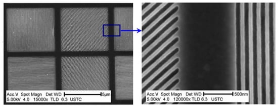
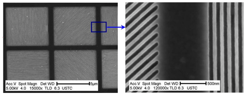
Pixelated polarization cameras that have emerged on the market over the past two decades have greatly improved the efficiency of polarization imaging. The core technology involves placing a pixel-sized polarizer made of a nano-grating in front of each pixel on the camera’s sensor [1,2]. Each group consists of four adjacent pixels arranged in the up, down, left, and right directions, with their grating orientations set at 0°, 45°, 90°, and 135°, respectively, as shown in Figure 1. The camera uses pixel groups with identical polarization orientations for image capture, enabling simultaneous acquisition of four polarized images at different angles.

Figure 1. Nano-grating polarizers made by micro-nano fabrication technology [1].

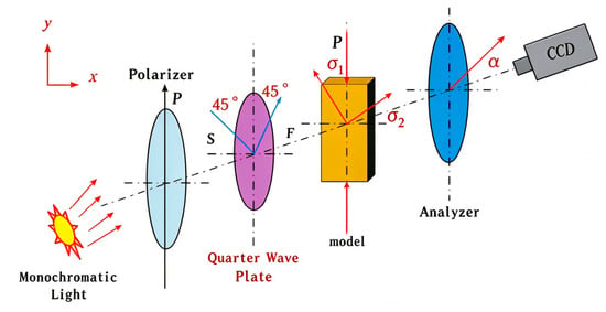
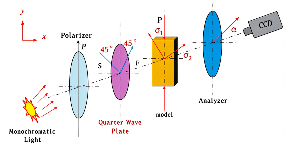
Pixelated polarization cameras have been introduced into digital photoelasticity owing to their capability for dynamic phase shifting. The photoelasticity method using a pixelated polarization camera generally adopts the optical setup shown in Figure 2. Compared with the conventional circular polariscope arrangement, this configuration removes the quarter-wave plate before the analyzer. Note that the incident light is circularly polarized before entering the specimen. If the azimuth angles of the polarization axis of the analyzer are rotated to 0°, 45°, 90°, and 135°, respectively, and the photoelasticity fringe fields recorded by the CCD camera at these angles are denoted as I₀, I₄₅, I₉₀, I₁₃₅, then according to the theory of polarization optics [3,4], we have

$$\begin{array}{l}{I}_{0^{°}}={\displaystyle \frac{1}{2}}(1-\sin 2\mathsf{\theta }\sin \mathsf{\delta }),I_{{45}^{°}}={\displaystyle \frac{1}{2}}(1+\cos 2\mathsf{\theta }\sin \mathsf{\delta })\\ I_{{90}^{°}}={\displaystyle \frac{1}{2}}(1+\sin 2\mathsf{\theta }\sin \mathsf{\delta }),I_{{135}^{°}}={\displaystyle \frac{1}{2}}(1-\cos 2\mathsf{\theta }\sin \mathsf{\delta })\end{array}$$

(1)

where δ is the phase retardation and θ is the angle of the principal stress of the model.

Figure 2. Schematic of the photoelasticity method using a pixelated polarization camera.

According to the definition of polarization optics, if we denote:

$$\begin{array}{l}{S}_0=I_{0^{°}}+I_{{90}^{°}}=1\\ S_1=I_{0^{°}}-I_{{90}^{°}}=-\sin 2\mathsf{\theta }\sin \mathsf{\delta }\\ S_2=I_{{45}^{°}}-I_{{135}^{°}}=\cos 2\mathsf{\theta }\sin \mathsf{\delta }\end{array}$$

(2)

Then the expression for the Degree of Linear Polarization (DoLP)—actually an incomplete expression with the element S3 missing—is:

$$\mathrm{DoLP}={\displaystyle \frac{\sqrt{S_1^2+S_2^2}}{S_0}}=\sin \mathsf{\delta }$$

(3)

With this approach, the phase retardation field of the specimen can be obtained directly from Equation (3). The pixelated polarization camera, in contrast, eliminates the need for both the analyzer and the rotating-analyzer procedure, allowing the images at the four polarization orientations to be captured in a single shot. This technique substantially improves the measurement efficiency of photoelasticity and offers other advantages over conventional photoelastic methods [5,6].

The grating polarizers shown in Figure 1 are fabricated using modern micro/nano fabrication techniques. Due to the limited accuracy of micro/nano fabrication processes, the period, width, and depth of the metallic nanowire gratings exhibit deviations of approximately 20% [7], causing the transmittance, extinction ratio, and polarization orientation of each polarization pixel to deviate from their design values. In addition, the non-uniform response of the individual pixels in the focal plane array, readout circuit offsets, and optical and electrical crosstalk between pixels further aggravate the non-uniformity of the polarization images [8]. Powell and Gruev [7] systematically investigated the calibration of pixelated polarization cameras and proposed both scalar and matrix calibration methods based on the mathematical model of the polarimeter: the scalar calibration corrects only the gain of each pixel, whereas the matrix calibration simultaneously corrects the transmittance and polarization orientation errors. Experimental results demonstrated that the matrix calibration is more effective in suppressing the errors in polarization image reconstruction. York and Gruev [8] took one pixel in a 2 × 2 superpixel as the reference and computed the gain and offset for the remaining three pixels, generating a pixel-by-pixel calibration matrix that can partially compensate for the errors introduced by readout circuit offsets as well as optical and electrical crosstalk. Zhang et al. [9] proposed a vector-form non-uniformity correction method, in which a correction matrix and an offset vector are calculated to correct the polarization images as a whole. Both simulations and experiments on real scenes demonstrated that the method can effectively suppress non-uniformity errors in the visible band. Huang et al. [10] jointly calibrated the transmittance of the polarization filters and the detector gain based on a redefined calculation of the DoLP, and the DoLP of the target was accurately recovered in both simulations and experiments. Feng et al. [11] established a performance model for the polarized pixels, describing the optoelectronic response of each pixel with three parameters: the major polarization responsivity, the minor polarization responsivity, and the polarization orientation. The polarization images were then calibrated based on this model, and the non-uniformity of the DoLP images was reduced to 6.79% of that of the uncalibrated images. Sun et al. [12] focused on the pixelated polarization camera and established a measurement model of the vector transfer matrix for pixel groups based on the nano-grating structure and the theory of polarized-light propagation. The optimal transfer matrix was fitted using the least-squares method, and pixel-level correction was implemented, reducing the camera non-uniformity from 2.00% to 0.26%, while the information entropy of the target DoLP image increased from 5.34 to 15.15.

Although considerable progress has been made in correcting fabrication errors, several issues still deserve further discussion. For example, do the correction parameters of the camera vary with the wavelength of the incident light? Are the correction parameters consistent among different polarization cameras of the same model? Moreover, the error evaluation and the correction parameters are typically obtained under a uniform, ideal linearly polarized light field, and the correction performance is characterized by parameters such as the DoLP. In photoelasticity tests, however, the phase retardation is more commonly used to evaluate the measurement errors, and circularly polarized light is more often adopted as the illumination. Therefore, whether the measurement accuracy of photoelasticity—especially that for the low-stress specimen—can be effectively improved after the pixelated polarization camera is corrected using the aforementioned methods remains to be examined. This paper focuses on addressing these issues.

2. Correction Algorithms for Pixelated Polarization Cameras

2.1. Polarization Characteristic Parameters of the Nano-Grating Polarizer

Taking the error evaluation and correction of the 0° grating polarizer as an example, its actual Mueller matrix elements deviate from the ideal values owing to manufacturing errors. Assuming that the elements of the first row of the Mueller matrix are given by A_f0, A_f1, A_f2, A_f3, the intensity of the incident light ${\overrightarrow{S}}_{\mathrm{in}}$ after passing through the 0° polarizer, as measured at pixel (i, j) on the target surface, can be expressed as follows:

$$I_0={\overrightarrow{A}}_f{\overrightarrow{S}}_{\mathrm{in}}+d=\left(\begin{array}{cc}{\overrightarrow{A}}_f& d\end{array}\right)\times (\begin{array}{cc}{\overrightarrow{S}}_{\mathrm{in}}& 1\end{array}{)}^{\top }$$

(4)

In the above equation, ${\overrightarrow{A}}_f$ is a vector represented by a 4 × 1 matrix (the four elements are A_f0, A_f1, A_f2, A_f3, which should be 1, cos2θ, sin2θ, and 0, respectively, under the ideal condition-i.e., infinite extinction ratio and accurate orientation of the polarization axis). ${\overrightarrow{S}}_{\mathrm{in}}$ is a Stokes vector of the linearly polarized incident light, which is represented by a 1 × 4 matrix, and has the specific expression 0.5 × (1, cos2θ, sin2θ, 0), with θ being the polarization angle. d is called the dark bias, and is a real correction that takes into account the factors of the photovoltaic conversion device. $\left(\begin{array}{cc}{\overrightarrow{A}}_f& d\end{array}\right)$ denotes that d is placed at the matrix tail of ${\overrightarrow{A}}_f$ to form a 1 × 5 matrix. $(\begin{array}{cc}{\overrightarrow{S}}_{\mathrm{in}}& 1\end{array}{)}^{\top }$ means that 1 is placed at the end of the matrix of ${\overrightarrow{S}}_{\mathrm{in}}$ to form a 1 × 5 matrix, which is then transposed.

${\overrightarrow{S}}_{\mathrm{in}}$ in Equation (4) can be artificially varied and precisely controlled, and $\left(\begin{array}{cc}{\overrightarrow{A}}_f& d\end{array}\right)$ has a total of 5 to-be-determined parameters describing the polarization and photoelectric conversion characteristics of the nano-grating at pixel (i,j). These 5 system parameters can be determined by the least squares method: by m (m > 5) times artificially changing ${\overrightarrow{S}}_{\mathrm{in}}$ (actually changing the polarization direction angle), recording the pixel values I_0,1, I_0,2, …, I_0,m at (i,j), and the 5 parameters that make Equation (5) take the minimum value are required.

$$I_{\mathrm{sum}}={\sum }_0^m{\left[{I_{0,\mathrm{m}}}_{(i,j)}-\left(\begin{array}{cc}{\overrightarrow{A}}_f& d\end{array}\right)\times (\begin{array}{cc}{\overrightarrow{S}}_{\mathrm{in},\mathrm{m}}& 1\end{array}{)}^{\top }\right]}^2$$

(5)

The least squares solution of the above equation can be expressed as:

$$\left(\begin{array}{cc}{\overrightarrow{A}}_f& d\end{array}\right)=\left(\begin{array}{ccc}{I}_1& \dots & I_m\end{array}\right){\left(\begin{array}{ccc}\begin{array}{c}{\overrightarrow{S}}_{\mathit{in},1}\\ 1\end{array}& \dots & \begin{array}{c}{\overrightarrow{S}}_{\mathit{in},m}\\ 1\end{array}\end{array}\right)}^{+}$$

(6)

where + denotes the pseudo-inverse matrix.

The parameters ${\overrightarrow{A}}_f$ and d corresponding to each pixel of I₀ can be determined using the above method. The method of determining the I₄₅ correction parameters is exactly similar to the previous step, except that I_0,1, I_0,2, …, I_0,m in Equation (5) should be replaced with I_45,1, I_45,2, …, I_45,m. The correction parameters of the polarization images at the other two angles are processed in the same way.

2.2. Correction Algorithms of Polarization Images with Errors

After determining the polarization parameters ${\overrightarrow{A}}_f$ and d for each nano-grating polarizer, the four measured polarization images I₀, I₄₅, I₉₀, I₁₃₅ were corrected to their “ideal state” as follows.

First, the polarization characteristic parameters of the pixels in the four images (i,j) are combined into two matrices A_sp and d_sp where:

$$A_{\mathit{sp}}=\left(\begin{array}{cccc}{A}_{0,f0}& A_{0,f1}& A_{0,f2}& A_{0,f3}\\ A_{45,f0}& A_{45,f1}& A_{45,f2}& A_{45,f3}\\ A_{90,f0}& A_{90,f1}& A_{90,f2}& A_{90,f3}\\ A_{135,f0}& A_{135,f1}& A_{135,f2}& A_{135,f3}\end{array}\right),d_{\mathit{sp}}=\left(\begin{array}{c}{d}_0\\ d_{45}\\ d_{90}\\ d_{135}\end{array}\right)$$

(7)

The first to fourth rows of the above equation are the ${\overrightarrow{A}}_f$ and d parameters of the pixels at position (i,j) for images I₀, I₄₅, I₉₀, I₁₃₅, respectively.

Second, the pixel values i₀, i₄₅, i₉₀, i₁₃₅ of the measured images I₀, I₄₅, I₉₀, I₁₃₅ at positions (i,j) are formed into a 4 × 1 matrix

$$I=\left(\begin{array}{c}{i}_0\\ i_{45}\\ i_{90}\\ i_{135}\end{array}\right)$$

(8)

The pixel values of the four measured sub-images at positions (i,j) are corrected to the ideal values $i_0^{\prime },i_{45}^{\prime },i_{90}^{\prime },i_{135}^{\prime }$ by the following equation:

$$I^{\prime }=\left(\begin{array}{c}{i}_0^{\prime }\\ i_{45}^{\prime }\\ i_{90}^{\prime }\\ i_{135}^{\prime }\end{array}\right)=\left(\begin{array}{cccc}1& 1& 0& 0\\ 1& 0& 1& 0\\ 1& -1& 0& 0\\ 1& 0& -1& 0\end{array}\right)A_{\mathit{sp}}^{+}(I-d_{\mathit{sp}})$$

(9)

where $A_{\mathit{sp}}^{+}$ is the pseudo-inverse matrix of the matrix A_sp in Equation (7).

More details of the correction algorithms can be found in refs. [7,13,14].

All the pixels of the four polarization images are corrected as described above, and the corrected images are then substituted into Equations (2) and (3) to obtain the corrected measurement results.

3. Assessment of Camera System Errors and Correction Effects

3.1. Experimental Program and Equipment

• Digital cameras and lens

Two pixelated polarization cameras based on the same image sensor, Sony IMX264MZR, with a full resolution of 2448 × 2048 × 8 bit, were employed; four polarization images with a resolution of 1224 × 1024 × 8 bit can be obtained in a single shot. In addition, an ordinary camera with a full resolution of 2448 × 2048 × 8 bit was used; in fact, the aforementioned pixelated polarization camera is developed from it by attaching a nano-grating polarizer in front of each pixel sensor. In this experiment, a polarizer with an extinction ratio of 10,000:1 was placed in front of the ordinary camera to mimic a polarization camera, and its polarization axis was set to four different angles (0°, 45°, 90°, and 135°) to acquire the four polarization images. These images were used to calculate the phase retardation of the specimen and the principal stress directions, and the results were compared with those obtained from the polarization camera images. In this paper, these three cameras are denoted as PolCCD1, PolCCD2, and NonPolCCD.

Residual stress in imaging lenses causes extra measurement errors. After testing, the Computar M3Z1228C-MP lens with low residual stress was chosen. To guarantee comparable test results, all three cameras in the experiment share this single imaging lens. Meanwhile, to reduce the influence of random camera noise, we adopted the software function to capture ten consecutive polarization images and perform averaging. The averaged image was used as the basis for phase retardation calculation.

B.

Circularly polarized light source

Photoelasticity based on pixelated polarization cameras requires circularly polarized incident light. Strictly circularly polarized light is usually obtained with polarization devices made of crystalline materials, the apertures of which are generally small (typically no more than 100 mm); large-aperture circular polarizers, on the other hand, are usually made of amorphous polymer materials, a typical example being the Edmund Optics polymer film CP42HE with an operating wavelength of 400–700 nm. Circular polarizers are commonly integrated into LED flat-panel light sources. In this experiment, two circularly polarized light sources were used, whose built-in circular polarizers are made of polymer film and quartz crystal, respectively (both 75 mm in diameter); they are hereafter referred to as the P-Source and the Q-Source. The quartz circular polarizer was designed and fabricated for a wavelength of 530 nm.

C.

Integral sphere and its settings

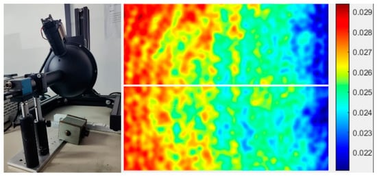
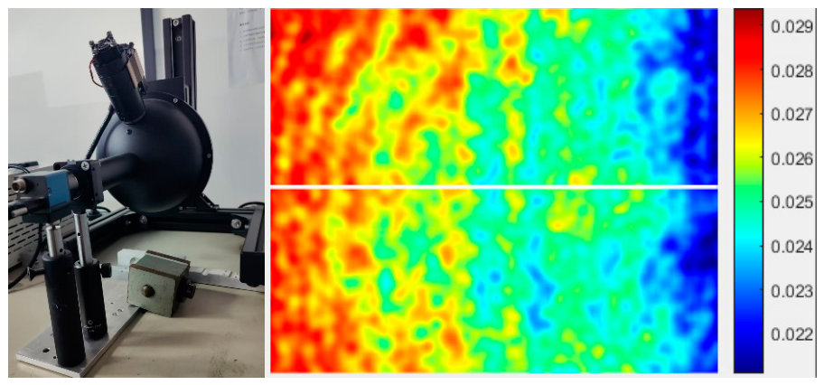
In the camera polarization parameter evaluation method described in Section 2, the light intensity incident on each pixel must be consistent. Therefore, stringent requirements are imposed on the uniformity and parallelism of the incident light. An integrating sphere is a common device for generating a uniform light field, and its internal light source is a halogen lamp with a broad spectral range of 200–2300 nm. The output port of the integrating sphere is connected to a collimator with an inner diameter of 22 mm. A lens group is mounted at the front end of the collimator to produce a parallel light beam, while a polarizer with an extinction ratio of approximately 10,000:1 and a diameter of 1 inch is placed at the rear end. The polarization direction of the outgoing light is adjusted by a graduated polarizer holder. A CCD without an imaging lens is positioned immediately behind the polarizer, such that the beam impinges perpendicularly and fully covers the target surface of the CCD. To avoid the influence of broadband light on measurement accuracy [6], a narrow-band filter is placed in front of the CCD target surface. In this experiment, the central working wavelengths of the narrow-band filters are 625 nm and 530 nm, respectively, both with a bandwidth of 10 nm. The polarization camera is fixed, and the polarizer is rotated to maximize the average gray value of the camera’s 0° image, which determines the 0° reference orientation of the polarizer. The entire experimental setup is shown in Figure 3. Before installing the high-extinction-ratio polarizer, four polarization images are captured to examine the polarization state of light emitted by the integrating sphere and calculate the degree of linear polarization (DoLP), as shown in Figure 3. It can be observed that the DoLP of the beam is close to 0, verifying the high uniformity and unpolarized characteristic of the light field from the integrating sphere.

Figure 3. Device for testing the camera correction parameters (left) and their uniformity (right).

3.2. Experimental Evaluation of Nano-Grating Polarizer Manufacturing Errors

• Verification of the Fabrication Errors of the Pixelated Polarization Camera

Theoretically, when the light field of the ideal circularly polarized source is used as the test object, the measured degree of linear polarization (DoLP) should be zero; when a standard quarter-wave plate is used as the test object, the measured DoLP should be 1.0, and the corresponding phase retardation should be 1.57 rad. The actual measured results thus reflect the level of the systematic errors.

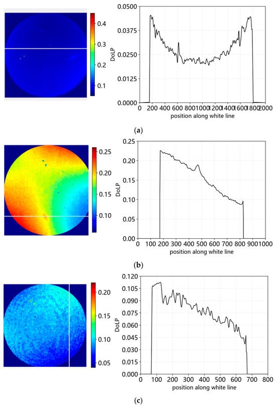
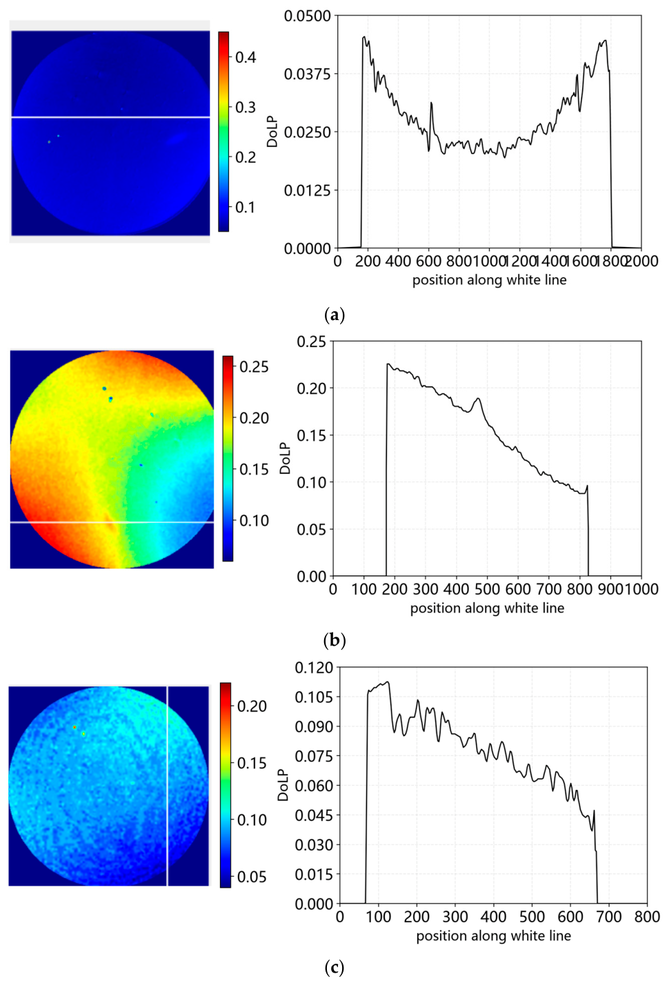
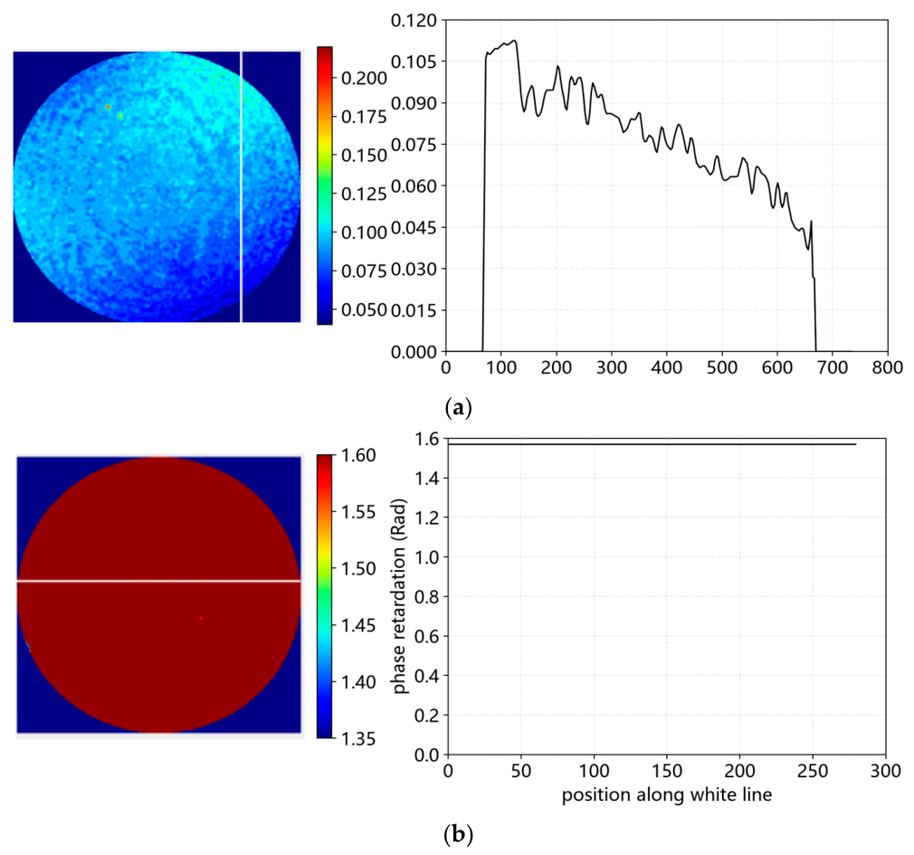
Figure 4a–c show the test results obtained with NonPolCCD, PolCCD1, and PolCCD2, respectively, using the same light source background (Q-source) as the test object. The curve on the right side of the figure shows the distribution of the DoLP field data (shown on the left) along the white line. It can be seen that the maximum value of DoLP of NonPolCCD is less than 0.05, which is close to the ideal value of zero. Whereas, the measured DoLP field distributions of PolCCD1 and PolCCD2 are not only inconsistent but also reach the maximum values of 0.25 and 0.105, respectively.

Figure 4. The phase 4. tardation test results of the three cameras for the same ideal circularly polarized background light source. (a) DoLP test results of Q-source with NonPolCCD. (b) DoLP test results of Q-source with PolCCD1. (c) DoLP test results of Q-source with PolCCD2.

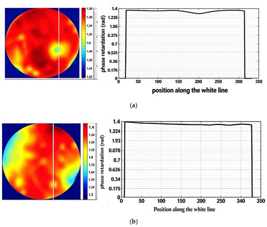
Figure 5a,b show the test results of the same achromatic quarter-wave plate measured with PolCCD1 and PolCCD2 under red light with a central wavelength of 625 nm. Although the DoLPs measured by both cameras are very close to the ideal value of 1.0, the phase retardation error is significant.

Figure 5. Polarization camera test of phase retardation field of several standard specimens. (a) Phase retardation test results of PolCCD1 on 1/4 waveplates. (b) Phase retardation test results of PolCCD2 on 1/4 waveplates.

The test conditions corresponding to Figure 4 and Figure 5 are exactly the same, and the difference in the results reflects the different intrinsic characteristics of the two pixelated polarization cameras. From these experimental results, it can be concluded that the nano-grating polarizer in the pixelated polarization camera does introduce systematic errors, and that the internal manufacturing errors are not identical even for cameras of the same model from the same manufacturer.

3.3. Polarization Parameters of the Pixelated Polarization Cameras

In the experimental setup described in the integral sphere and its settings, the axis angle of the polarizer is set to 0°, 10°, …, 170°, yielding 18 positions in total (i.e., m = 18) in Equations (5) and (6). Ten consecutive images are captured at each angle and averaged to obtain the final measurement at that angle, resulting in a total of 4 × 18 images. Equation (6) is adopted to calculate the characteristic parameters of each pixelated polarizer, and Equation (9) is further used to correct the raw acquired images.

We measured the polarization characteristic parameters of two pixelated polarization cameras, PolCCD1 and PolCCD2. All experimental equipment and technical settings remain identical except for the cameras themselves.

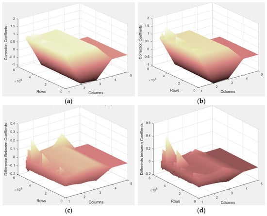
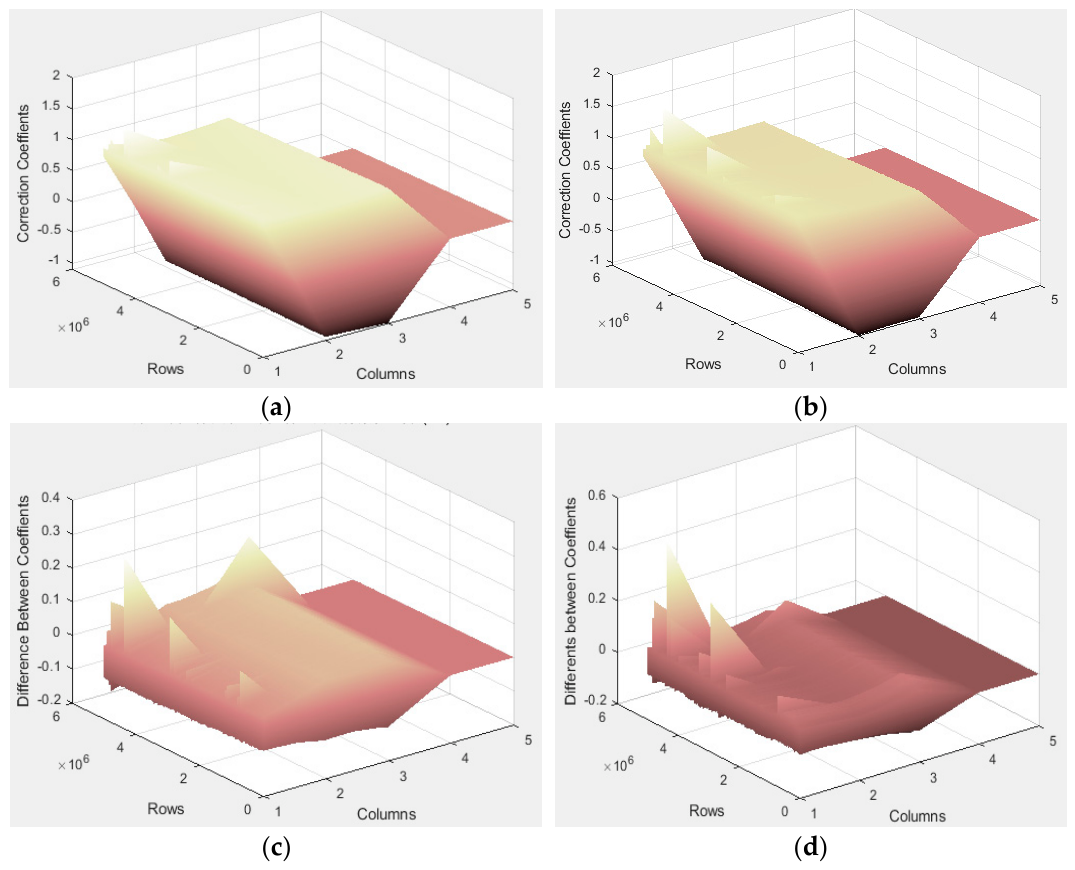
Figure 6a,b illustrate the 3D distributions of polarization parameters of PolCCD1 under red and green illumination, respectively. The columns correspond to five polarization parameters $\left(\begin{array}{cc}{\overrightarrow{A}}_f& d\end{array}\right)$ and the rows represent all pixels of PolCCD1, amounting to 2448 × 2048 points. It can be observed from the two subfigures that the parameter values of PolCCD1 generally fall within the range of (−1, 1) and do not deviate significantly from their ideal values. Nevertheless, local anomalies exist in the calibrated parameters of the camera, which may originate from severe defects on the micro-nano polarizer. Figure 6c shows the differences in polarization parameters of the same camera under different wavelengths of light, which are roughly within 0.2. In contrast, Figure 6d presents the differences in polarization parameters between the two cameras under illumination of the same wavelength, which are also approximately within 0.2.

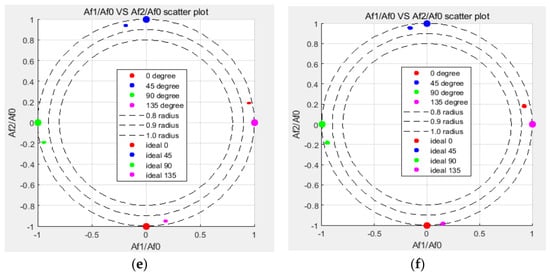
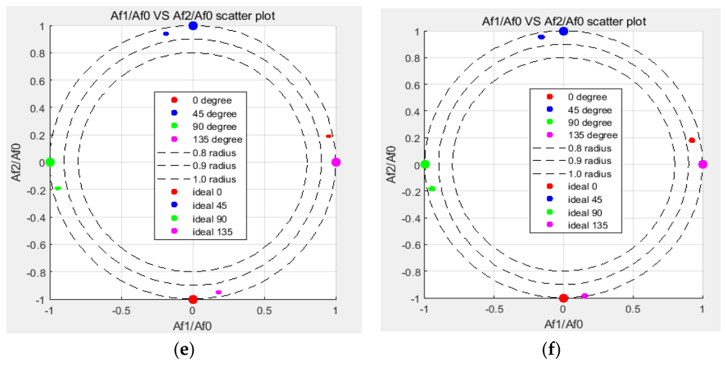
Figure 6. Test results of polarization parameters of two polarization cameras. (a) Distribution of the correction parameters of PolCCD1 under red light. (b) Distribution of the correction parameters of PolCCD1 under green light. (c) Difference in correction parameters of PolCCD1 under red & green light. (d) Difference in correction parameters of PolCCD 1&2 under red light. (e) Correction factor statistics for PolCCD1. (f) Correction factor statistics for PolCCD2.

Figure 6e,f show the statistical results of the correction coefficients of the two cameras, with the horizontal and vertical axes being A_f1/A_f0 and A_f2/A_f0, respectively. For the ideal polarization directions of 0°, 45°, 90°, and 135°, the ideal values of A_f1/A_f0 (=sin2θ) are 0, 1, 0, and −1, respectively, and those of A_f2/A_f0 (=cos2θ) are 1, 0, −1, and 0, respectively; their positions correspond to the four large dots of different colors in Figure 6e and Figure 6f, respectively. A total of 2448 × 2048 pixels are plotted in each of Figure 6e,f, and the corresponding statistical results are also presented in the two figures. As can be seen, although the polarization parameters of the nano-grating polarizers deviate from the ideal values, indicating problems in the fabrication accuracy, the distribution of the polarization parameters of each nano-grating polarizer is highly concentrated, which suggests that the deviation in fabrication quality is very small.

3.4. Effect of Camera Correction on the Accuracy of Photoelasticity Measurements

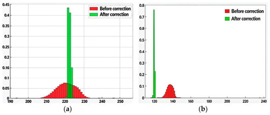
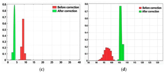
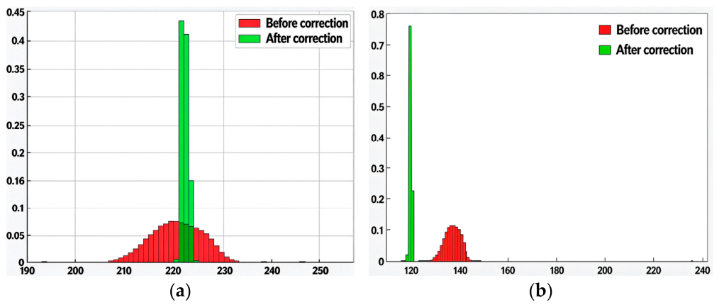
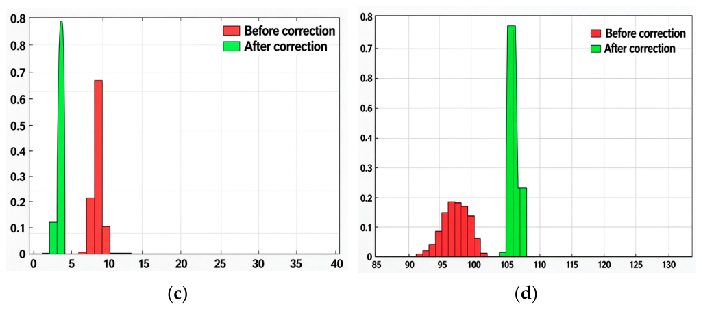
A set of polarization images of PolCCD2 was recorded during the polarization-parameter calibration test (where the polarizer angle was set to 0°, green light), and these images were then corrected using the algorithm introduced in Section 2. To observe the correction effect more intuitively and conveniently, the histograms of the two sets of images (before and after correction) were computed, as shown in Figure 7a–d. Two features can be clearly seen: first, the gray-value distribution of the corrected images is more concentrated; second, the peak gray values of the corrected images are shifted relative to those of the original images, the shift being most obvious for the 45° and 135° polarization images, with an offset of nearly 20 gray levels. After correction, the gray levels of the four polarization images tend to be consistent, which is in line with theoretical expectations. The large gray-level deviation of the original images should be attributed to the orientation error of the nano-grating polarizer, because the light intensity is most sensitive to the variation in the polarization angle near the ±45° orientations.

Figure 7. Comparison of the effect of the original map used to test the polarization parameters of the camera before and after correction. (a) Histogram statistics before and after correction for 0° polarized images. (b) Histogram statistics before and after correction for 45° polarized images. (c) Histogram statistics before and after correction for 90° polarized images. (d) Histogram statistics before and after correction for 135° polarized images.

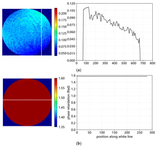
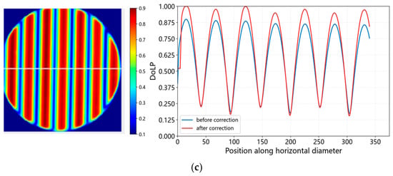
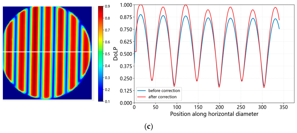
We next corrected the background images of the Q-source and recalculated the phase retardation of the light source; the results are shown in Figure 8a. Compared with the results before correction shown in Figure 4c, no significant improvement is observed. We then corrected the polarization images of the standard quarter-wave plate and recalculated the phase retardation field; the result is shown in Figure 8b, where the corrected phase retardation is uniformly distributed, as expected (i.e., 1.57 rad).

Figure 8. Test results of the standard specimen after using the correction algorithm. (a) After correcting the 4 polarized images, PolCCD2 re-tested the phase retardation of the source background. (b) After correcting the 4 polarized images, PolCCD2 re-tested the phase retardation of the 1/4 wave plate. (c) The DoLP test results of PolCCD2 for the special wave plate under the P-Source before and after correction.

Left of Figure 8c presents the measured DoLP of PolCCD2 for a specially fabricated waveplate under the P-Source. The phase retardation δ of this waveplate varies continuously from 0 to 6π along the horizontal diameter (designed for a wavelength of 550 nm). According to Equation (3), the DoLP should vary sinusoidally along this diameter, ideally reaching a maximum of 1.0 at δ = nπ/2 with n odd and a minimum of 0.0 at δ = nπ/2 with n even. However, due to polarization errors of the light source and fabrication errors of the camera, the measured DoLP falls short of these ideal values, as indicated by the blue curve on the right of Figure 8c. After correcting the acquired polarization images of this waveplate, the DoLP field was recalculated, yielding the red curve. Comparison of the two curves reveals that the peaks of the red curve are enhanced—the first two peaks even reaching the ideal value of 1.0—whereas the troughs remain essentially unchanged.

The left of Figure 8c shows the DoLP test results of PolCCD2 for a specially fabricated waveplate under the P-Source. The phase retardation δ of this waveplate varies continuously from 0 to 6π from left to right along the horizontal diameter (designed for a wavelength of 550 nm). According to Equation (3), its DoLP should vary sinusoidally along the horizontal diameter, reaching maxima of ideally 1.0 at δ = nπ/2 with n odd, and minima of ideally 0.0 at δ = nπ/2 with n even. Owing to the polarization errors of the light source and the fabrication errors of the camera, the measured DoLP does not reach the desired values (as indicated as the blue curve in the right). However, after correcting the polarization image of this waveplate, the DoLP field was recalculated, as shown the red curve in the right of Figure 8c. Comparing the two curves, it can be seen that the peaks of the curve are strengthened—the first two peaks even reaching the ideal value of 1.0—while the troughs remain essentially unchanged.

From the results in Figure 8, it can be seen that the correction algorithm improves the measurement accuracy of photoelasticity to a certain extent, but its effectiveness is limited to cases with relatively high DoLP; on the other hand, it is almost ineffective for cases where the DoLP or the stress level is relatively low.

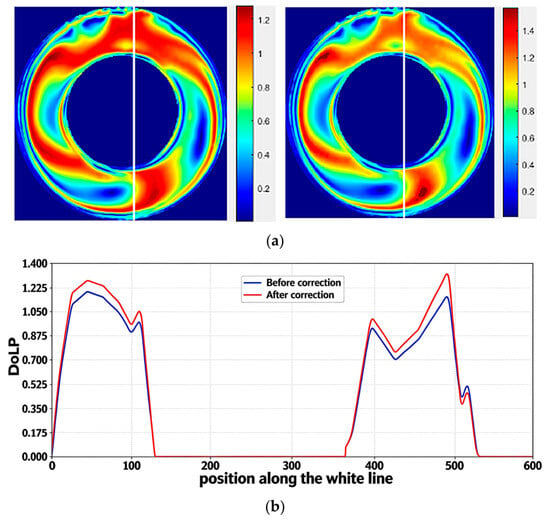
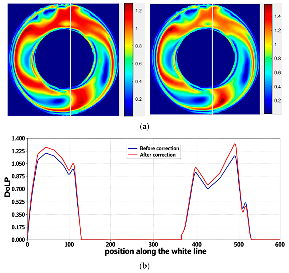
An example shown in Figure 9 further supports this conclusion: a polycarbonate resin ring containing residual stress induced by machining was used as the specimen. Its DoLP distribution was recorded with PolCCD2, as shown on the left of Figure 9a; after correcting the polarization images, the DoLP was recalculated, as shown on the right of Figure 9a. The DoLP distribution curve along the same path before and after correction is shown in Figure 9b. It can be seen that the correction does not change the distribution pattern of the DoLP and phase retardation, but the regions with relatively high retardation are strengthened, whereas those with relatively low retardation remain weak and almost unchanged. In other words, the present correction algorithm can effectively improve the contrast of the DoLP images, which is beneficial for applications such as polarization imaging and defogging; the application example given at the end of Powell’s paper [7] belongs to this category. However, in applications such as the testing of low or tiny stress birefringence, the algorithm is of very limited help in improving the measurement accuracy of photoelasticity.

Figure 9. Comparison of residual stress test results for a polycarbonate numerical ring: before correction (a) and after correction (b). (a) Phase retardation field measurements, before (left) and after (right) correction. (b) DoLP distribution curves along the same path before (left) and after (right) correction.

4. Summary and Conclusions

Numerous factors affect the measurement accuracy of the novel photoelasticity [6]. This paper focuses on one of these factors, namely the influence of manufacturing errors of the nano-grating polarizer on photoelasticity measurement accuracy, together with a study on the effectiveness of the corresponding correction algorithm. In this study, to enhance the comparability and reliability of the experimental data, the experimental conditions for the different cameras were kept as consistent as possible.

The existence of manufacturing errors was first verified experimentally; a software correction algorithm proposed in the literature was then implemented to correct the polarization images, and a series of experiments was carried out to evaluate the effect of the correction. The following conclusions can be drawn.

(1)

Pixelated polarization cameras indeed suffer from manufacturing errors, which are not identical even among cameras of the same model from the same manufacturer. With the same ideal circularly polarized background (Q-source) as the test object, the measured DoLP of the ordinary camera NonPolCCD remained below 0.05, whereas those of PolCCD1 and PolCCD2 were not only inconsistent in distribution but also reached maximum values of 0.25 and 0.105, respectively. In the quarter-wave plate test, although the DoLP measured by both polarization cameras was close to the ideal value of 1.0, the phase retardation errors were significant. These results directly confirm that the nano-grating polarizers integrated in pixelated polarization cameras introduce systematic errors. Therefore, each camera must be calibrated individually before use; moreover, the calibration parameters of the same camera also vary with wavelength.

(2)

The software correction algorithm proposed in the literature can effectively correct the polarization images, but only for data with high DoLP. After correction, the gray-value distributions of the four polarization images become more concentrated and consistent, and the DoLP degraded by the low extinction ratio of the nano-grating polarizer (attributable to non-ideal fabrication) can be restored to the normal level; for the specially fabricated waveplate, the first two peaks of the DoLP curve even reached the ideal value of 1.0.

(3)

The correction algorithm has no significant corrective effect on data with low DoLP. This characteristic stems from the fact that the correction parameters are calibrated in an environment where the DoLP is close to 1.0. Consequently, the algorithm can effectively enhance the contrast of DoLP images, which is beneficial for applications such as polarization imaging and defogging, but its effectiveness in improving the measurement accuracy of photoelasticity is rather limited, especially for specimens with low stress or low stress birefringence: the correction does not change the distribution pattern of the phase retardation field, and the regions with relatively low retardation remain almost unchanged.

(4)

The polarization characteristic parameters of different cameras can differ by about 20%, and the correction parameters are not transferable between cameras; calibration and correction must therefore be performed individually for each camera.

The above findings can provide guidance for photoelasticity measurements using pixelated polarization cameras. Nevertheless, in the studies described above, we did not account for the influence of thermal drift on the camera sensor. It is widely recognized that the novel photoelasticity based on pixelated polarization cameras yields limited measurement accuracy for low-stress specimens, and the correction algorithm proposed in this paper offers only marginal improvement in accuracy for such specimens. How to address these issues still requires further investigation.

References

- Zhang, Z.; Dong, F.; Cheng, T.; Qiu, K.; Zhang, Q.; Chu, W.; Wu, X. Nano-fabricated pixelated micropolarizer array for visible imaging polarimetry. Rev. Sci. Instrum. 2014, 85, 105002. [Google Scholar] [CrossRef] [Scilit] [PubMed]
- Zhou, Y.L.; David, J.K. Design and parallel fabrication of wire-grid polarization arrays for polarization-resolved imaging at 1.55 μm. Appl. Opt. 2008, 47, 3555–3560. [Google Scholar] [CrossRef] [Scilit] [PubMed]
- Goldstein, D.H. Light; CRC Press: Boca Raton, FL, USA, 2017. [Google Scholar]
- Kliger, D.S.; James, W.L. Polarized Light in Optics and Spectroscopy; Elsevier: Amsterdam, The Netherlands, 2012. [Google Scholar]
- Su, F.; Wu, S.H.; Zhang, Z. A brief review of the photoelasticity based on a pixelated polarization camera: Principle, advantges/disadvantages and typical applications. J. Mech. 2024, 40, 698–710. [Google Scholar] [CrossRef] [Scilit]
- Su, F.; Wang, Z.J. Error analysis and correction of a photoelastic method based on a pixelated polarization camera. Opt. Lasers Eng. 2023, 161, 107374. [Google Scholar] [CrossRef] [Scilit]
- Powell, S.B.; Gruev, V. Calibration methods for division-of-focal-plane polarimeters. Opt. Express 2013, 21, 21039–21055. [Google Scholar] [CrossRef] [Scilit] [PubMed]
- York, T.; Gruev, V. Calibration method for division of focal plane polarimeters in the optical and near infrared regime. In Proceedings of the SPIE 8012: Infrared Technology and Applications XXXVII; SPIE: Bellingham, WA, USA, 2011; Volume 80120. [Google Scholar]
- Zhang, J.; Luo, H.; Hui, B.; Chang, Z. Non-uniformity correction for division of focal plane polarimeters with a calibration method. Appl. Opt. 2016, 55, 7236–7242. [Google Scholar] [CrossRef] [Scilit] [PubMed]
- Fei, H.; Li, F.M.; Chen, W.C.; Zhang, R.; Chen, C.S. Calibration method for division of focal plane polarimeters. Appl. Opt. 2018, 57, 4992–4999. [Google Scholar] [CrossRef] [Scilit] [PubMed]
- Feng, B.; Shi, Z.; Liu, H.; Liu, L.; Zhao, Y.; Zhang, J. Polarized-pixel performance model for DoFP polarimeter. J. Opt. 2018, 20, 065703. [Google Scholar] [CrossRef] [Scilit]
- Sun, H.; Wang, D.J.; Ma, T.X.; Xu, W.; Yao, Y. High-precision pixel-level polarization non-uniformity correction for pixelated grating polarization cameras. Acta Opt. Sin. 2017, 37, 1111002. [Google Scholar]
- Giménez, Y.; Lapray, P.J.; Foulonneau, A.; Bigué, L. Calibration algorithms for polarization filter array camera: Survey and evaluation. J. Electron. Imaging 2020, 29, 041011. [Google Scholar] [CrossRef] [Scilit]
- Lane, C.; Rode, D.; Rösgen, T. Calibration of a polarization image sensor and investigation of influencing factors. Appl. Opt. 2022, 61, C37–C45. [Google Scholar] [CrossRef] [Scilit] [PubMed]
Disclaimer/Publisher’s Note: The statements, opinions and data contained in all publications are solely those of the individual author(s) and contributor(s) and not of MDPI and/or the editor(s). MDPI and/or the editor(s) disclaim responsibility for any injury to people or property resulting from any ideas, methods, instructions or products referred to in the content. |
© 2026 by the authors. Licensee MDPI, Basel, Switzerland. This article is an open access article distributed under the terms and conditions of the Creative Commons Attribution (CC BY) license.