Self-Supervised Deep Learning for Attosecond and Femtosecond Pulse Reconstruction

Abstract

The retrieval of attosecond and femtosecond pulses from attosecond streaking spectrograms is a high-dimensional ill-posed inverse problem. The traditional FROG CRAB (frequency-resolved optical gating for complete reconstruction of attosecond bursts) method relies on the central momentum approximation, while supervised deep learning is constrained by the scarcity of labeled samples and lacks interpretability. In this paper, we propose a self-supervised collaborative reconstruction framework incorporating physics-based constraints, which integrates light-field representation, a differentiable physical model, and a prior regularization module. This framework requires only a small number of unlabeled samples for training and performs direct inference, thereby achieving collaborative high-precision retrieval of attosecond extreme ultraviolet (XUV) and femtosecond infrared pulses. Reconstructions from simulated and measured streaking spectrograms demonstrate that, compared to FROG CRAB, our self-supervised approach is more accurate even for extremely low signal-to-noise ratios, offering a novel, intelligent reconstruction solution for attosecond metrology with limited data and low photon flux.

1. Introduction

Since the advent of attosecond laser technology, attosecond XUV and femtosecond infrared pulses have formed the core instrumental foundation of attosecond metrology and are widely employed in cutting-edge fields such as atomic and molecular electronic dynamics, photochemical reactions, and ultrafast processes in condensed matter [1,2]. As key observable data for characterizing pulses and probing electron dynamics, attosecond photoelectron spectrograms contain the time-domain envelope, amplitude, and phase information of ultrashort light fields, serving as the crucial basis for precise pulse reconstruction [3]. Accurately retrieving the pulse distributions of both attosecond XUV and femtosecond infrared fields is of great significance for unraveling photoionization processes, manipulating electron wave packets, and enhancing the quality of attosecond light sources [4]. Recent advances in attosecond streaking have demonstrated its applicability in the water window [5] and for ultra-short soft X-ray pulses [6]. High-repetition-rate attosecond sources [7] have enabled streaking measurements with improved signal-to-noise ratio, and advanced pulse retrieval methods [8] have further motivated the development of robust reconstruction algorithms. However, achieving high-precision reconstruction still faces severe challenges. The inversion algorithms used for attosecond streaking spectrogram have inherent ill-conditioned characteristics: the broadband nature of XUV pulses undermines the central momentum approximation upon which FROG CRAB relies; moreover, in soft X-ray experiments within the water window, the photon yield is extremely low, leading to strong Poisson statistical noise accompanying the streaking traces [9].

The attosecond streaking camera is currently the most widely used experimental measurement technique for characterizing isolated attosecond pulses [10]. For the theoretical inversion of streaking spectrograms, this approach builds a physical model linking attosecond pulses to a photoelectron spectrogram based on the Schrödinger equation. By minimizing an error function that quantifies the discrepancy between the theoretically simulated and experimentally measured streaking spectrograms, the method iteratively optimizes and retrieves the phase of the attosecond pulse [11,12]. Mairesse and Quéré drew inspiration from femtosecond FROG theory and proposed the FROG CRAB iterative algorithm [13], extending frequency-resolved optical gating to the XUV regime and solving for both the attosecond pulse and the gating pulse via generalized projection iteration [14]. This method introduces the central momentum approximation, which leads to the severe loss of high-frequency phase information in broadband XUV scenarios due to the breakdown of this assumption. To circumvent the limitations of the central momentum approximation, the PROOF (phase retrieval by omega oscillation filtering) algorithm performs a Taylor expansion of the streaking spectrogram according to the frequency of the dressing laser field [15]. However, this approach is applicable only under the condition of a relatively weak dressing field. Other methods either involve computationally intensive iterative procedures [16] or can only retrieve the phase information of the attosecond pulse [17,18]. The all-optical in situ reconstruction scheme enables pulse characterization without requiring photoelectron detection [19,20]. Yet, it can only measure the attosecond pulse information at the point of its generation rather than at the application site, thus limiting its applicability. Supervised neural networks used for streaking spectrogram inversion rely on massive paired datasets for training, seeking to establish a mapping function between streaking the spectrogram and attosecond pulse. Such inversion approaches often suffer from insufficient model generalization [21]. The attosecond pulse retrieval scheme based on conditional variational generative networks [22,23] constructs a separately trained generative model to approximate the prior signal. Similarly, it requires the prior construction of a large-scale dataset comprising matched pulse parameter and streaking spectrogram pairs.

In response to the above-mentioned issues, this paper was inspired by a tomographic reconstruction algorithm based on self-supervised learning [24] and proposes a collaborative deep learning framework for reconstruction that embeds a differentiable physical model. This framework abandons the central momentum approximation, integrates a Gaussian random Fourier feature module that fully preserves the high-frequency details of the pulse, and includes a dual-regularization module that enforces constraints to optimize the pulse structure. With only a very small number of unlabeled samples required for training—or even without any training at all—this algorithm can retrieve attosecond and femtosecond pulses with high precision from attosecond streaking spectrograms even with extremely low signal-to-noise ratios.

2. Research Methodology

The algorithm presented in this paper takes the attosecond time-resolved photoelectron spectrogram as its sole input and performs end-to-end co-reconstruction of attosecond XUV and femtosecond infrared pulses. The overall framework is divided into three major modules: light-field distribution prediction, differentiable projection, and regularized optimization.

The light-field distribution prediction module is a self-supervised end-to-end network consisting of three parts: an input layer, a Fourier feature projection layer, and hidden layers. Its core function is to establish a mapping relationship between 3D coordinates and the discrete light field. The network input comprises 3D coordinate points $p_i=(x_i,y_i,z_i)(i=1,2,\dots ,N_E)$, where $N_E$ represents the total number of pixels in the discretized light field. The network learns a mapping function $F_{\mathrm{\Theta }}$ that transforms coordinates into light-field amplitudes:

$$F_{\mathrm{\Theta }}\left(p_i\right)=E_i,i=1,2,\dots ,N_E$$

(1)

where $\mathrm{\Theta }$ represents all learnable parameters of the network, and $E_i$ denotes the discrete value of the reconstructed light field at the location corresponding to coordinate $p_i$.

Low-dimensional coordinate inputs struggle to capture the fine temporal details of high-frequency pulse signals. Therefore, we introduce Gaussian random Fourier feature projection [25] to map low-dimensional coordinates into a high-dimensional feature space, thereby enhancing the network’s ability to represent high-frequency signals. The mapping formula is as follows:

$$\mathcal{M}\left(p_i\right)=\left(sin2\pi ·B·p_i,cos2\pi ·B·p_i\right)$$

(2)

where the frequency vector B is randomly sampled from a Gaussian distribution $N(0,{\sigma }^2)$, and the hyperparameter $\sigma$ controls the range of signal frequencies that the network can represent. If $\sigma$ is too small, the reconstructed light field becomes overly smooth and loses fine details. If $\sigma$ is too large, it may lead to overfitting and noise amplification. Therefore, this parameter needs to be individually optimized for different pulse reconstruction tasks. This layer is crucial for achieving high-frequency detail reconstruction of ultrashort pulses.

The hidden layers adopt a seven-layer fully connected MLP architecture: the first six layers each contain 256 neurons, and the last layer is equipped with a single neuron to output the scalar amplitude of the light field. A Swish activation function is used between consecutive layers, providing enhanced nonlinear fitting capability. The output of the last layer is paired with a Sigmoid activation function to constrain the range of the light-field amplitude. The Sigmoid function constrains the network output to $[0,1]$, which is then linearly mapped to $[-1,1]$ to allow the electric field to take negative values. The overall amplitude is scaled according to the maximum signal in the input spectrogram. The MLP takes the Fourier feature vector $\mathcal{M}\left(p_i\right)$ as input and predicts the corresponding light-field $E_i$ at each coordinate point.

The differentiable projection module transforms the light field E predicted by the network forward into a synthetic photoelectron spectrogram, thereby completing the physical projection from light field to photoelectron spectrogram. This layer establishes the backpropagation loss pathway for self-supervised training, ensuring that the network’s training adheres to physical laws. Guided by the physical generation model of the photoelectron spectrogram, this module is central to enforcing physical constraints. By adding different levels of Poisson noise to the sample data and randomly applying global masking to the input spectral data during training, the process simulates the signal loss and random noise encountered in experiments, compelling the network to learn the intrinsic features of the light field and enhancing its stability under complex experimental conditions.

The light field initially reconstructed via the network still exhibits subtle distortions in its time-domain geometric structure. To address this issue, we designed a geometric regularization module that integrates both local prior information (total variation, TV) and non-local prior information (non-local mean, NLM) [26,27]. The total variation regularization $\mathrm{TV}\left(E\right)$ (a local prior) enforces local smoothness of the light field, effectively suppressing noise at pulse edges and eliminating jagged distortions. Meanwhile, the non-local mean regularization $\mathrm{NLM}\left(E\right)$ (a non-local prior) exploits globally similar structures within the light field, correcting global geometric distortions while preserving the overall shape of the pulses.

The total loss function for the self-supervised algorithm is as follows:

$$L=\parallel S_{\mathrm{model}}\left(E\right)-S_{\mathrm{raw}}{\parallel }_2^2+W·\parallel S_{\mathrm{model}}\left(E\right)-S_{\mathrm{proj}}\left(E\right){\parallel }_2^2+k_1·\mathrm{TV}\left(E\right)+k_2·\mathrm{NLM}\left(E\right)$$

(3)

where $S_{\mathrm{model}}$ is the photoelectron spectrogram calculated by the physical generation model, $S_{\mathrm{proj}}$ is the photoelectron spectrogram output by the differentiable projection layer, and $S_{\mathrm{raw}}$ is the raw input reference attosecond photoelectron spectrogram. The network updates its parameters by minimizing the loss function. The first term ($\parallel S_{\mathrm{model}}\left(E\right)-S_{\mathrm{raw}}{\parallel }_2^2$) is the data fidelity term, ensuring that the physically simulated spectrogram matches the raw input spectrogram. The second term ($\parallel S_{\mathrm{model}}\left(E\right)-S_{\mathrm{proj}}{\left(E\right)\parallel }_2^2$) is the model consistency term, which forces the differentiable projection layer to be consistent with the physical generation model, thereby learning the underlying physical mechanisms governing photoelectron spectrogram generation. The third and fourth terms are the TV and NLM regularization terms, respectively. The first two terms jointly ensure that the network framework simultaneously optimizes the light-field reconstruction and the physical consistency of the projection. W is a confidence weight matrix whose elements range from $[0,1]$, controlling the relative weights of the two loss terms. In this paper, we set W to $0.5$. $k_1$ and $k_2$ are the weight coefficients for the two types of regularization terms, which in this paper are set to $0.1$ and $0.1$, respectively. The optimization solver employs a forward–backward splitting iterative algorithm, using the randomly initialized light field produced by the network as the initial value and iteratively updating until convergence. This module is highly flexible and can be extended with additional physical regularization terms according to task requirements.

3. Results and Analysis

3.1. Training Settings

Due to the scarcity of attosecond time-resolved photoelectron spectrogram datasets, we used simulated data as training samples. During the inference phase, either simulated or experimental data can be used. The simulated samples were generated using the strong-field approximation model [28,29] to compute the attosecond streaking photoelectron spectrogram of hydrogen atoms. The physical model for the photoelectron spectrogram also employs the strong-field approximation model. The simulated data underwent global masking and were further corrupted with Poisson noise. Both the attosecond XUV and the femtosecond infrared pulse envelopes had Gaussian profiles.

In the simulated samples, the central energies of the XUV photons were $15\omega$ and $41\omega$ (where $\hslash \omega =1.55$ eV, the central energy of infrared photons), with pulse widths of approximately 0.73 fs and 1.21 fs, respectively. The femtosecond infrared pulses had pulse widths of approximately 7.26 fs and 12.10 fs, and their carrier-envelope phases were 0 and $\pi /2$, respectively. Poisson noise ($\lambda =20$ and 100) was added to the peak-normalized attosecond time-resolved photoelectron spectrogram samples, where the parameter $\lambda$ is the average peak count of the Poisson distribution. We extracted 22 samples from the simulation data as the training set and another four samples from the same dataset as part of the inference set. The 26 spectrograms were generated by varying the IR pulse width (7.26 fs and 12.10 fs), CEP (0 and $\pi /2$), XUV pulse width (0.73 fs and 1.21 fs), and noise level ($\lambda =20$ and 100). The remaining part of the inference set consisted of four additional samples with more severe Poisson noise ($\lambda =5$ and 10). These four samples, whose noise levels were not present in the training set, were used to test the generalization capability of the reconstruction algorithm in suppressing noise, as shown in Table 1. This method can be applied either with prior training followed by inference—referred to as SSD (self-supervised deep learning), or directly without any training—referred to as SSD w/oT (without training). On an NVIDIA V100 GPU, the inference time for SSD was approximately 1 min, while the inference time for SSD w/oT was about 3 min.

Table 1. Cosine similarity of retrieved light pulses under different Poisson noise levels and final-state center energies.

	FROG CRAB	SSD w/oT	SSD
	[XUV, IR]	[XUV, IR]	[XUV, IR]
$9.65$ eV, without noise	0.9832, 0.9928	0.9926, 0.9940	0.9991, 0.9947
$9.65$ eV, with $\lambda =20$	0.9457, 0.9372	0.9911, 0.9892	0.9987, 0.9934
$9.65$ eV, with $\lambda =10$	0.9415, 0.9148	0.9902, 0.9859	0.9984, 0.9930
$9.65$ eV, with $\lambda =5$	0.9381, 0.8908	0.9895, 0.9838	0.9982, 0.9928
$49.95$ eV, without noise	0.9988, 0.9946	0.9993, 0.9971	0.9998, 0.9994
$49.95$ eV, with $\lambda =20$	0.9970, 0.9728	0.9991, 0.9962	0.9997, 0.9991
$49.95$ eV, with $\lambda =10$	0.9951, 0.9652	0.9985, 0.9941	0.9995, 0.9983
$49.95$ eV, with $\lambda =5$	0.9935, 0.9591	0.9973, 0.9912	0.9992, 0.9972

We note that while the simulated training data used hydrogen for the SFA model, the experimental data in Section 3.3 used neon atoms, demonstrating that the approach is applicable to multi-electron atoms. For more accurate reconstructions with multi-electron atoms, the differentiable physical model can be extended to include energy-dependent dipole matrix elements [30].

3.2. Reconstruction Results from Simulations

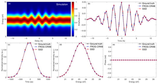
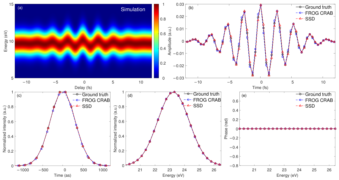
The retrieved attosecond and femtosecond pulse results from the noise-free simulated attosecond streaking spectrogram are shown in Figure 1. The femtosecond pulse retrieved by SSD closely matches the ground truth, whereas the femtosecond pulse retrieved by FROG CRAB exhibits a smaller amplitude compared to the ground truth. Both methods yield attosecond pulses that closely match the ground truth in terms of envelope, spectral intensity, and phase.

Figure 1. Retrieval of light pulses from noise-free simulated attosecond streaking spectrogram. (a) Input simulated attosecond streaking spectrogram. (b) Comparison of femtosecond pulses. (c–e) Characterization of attosecond pulses: (c) temporal intensity profile, (d) spectral intensity distribution, and (e) spectral phase distribution. Results obtained by FROG CRAB and SSD are compared with ground truth.

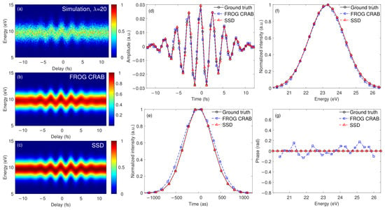
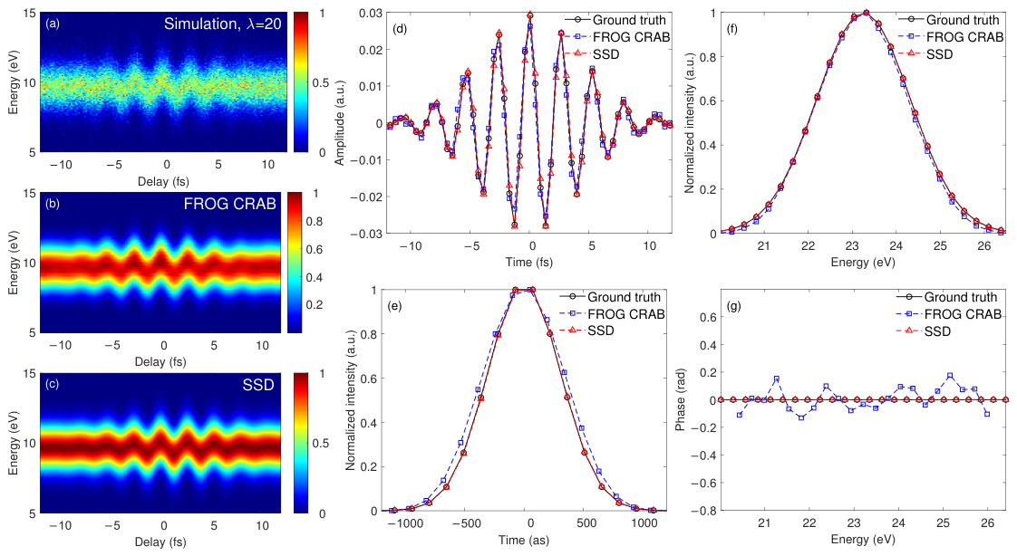
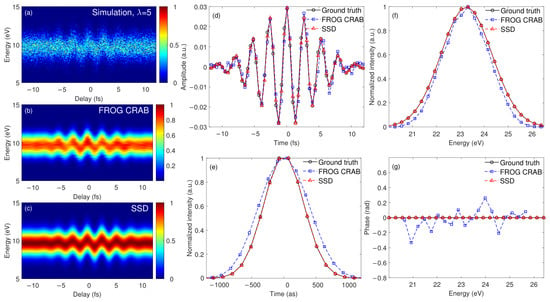
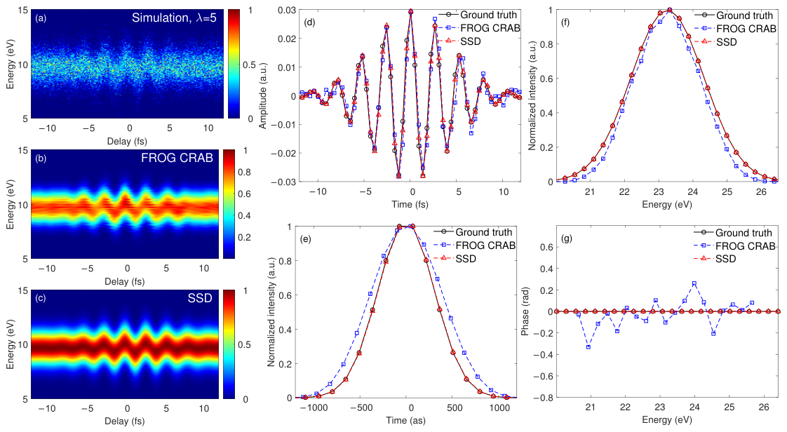
For the attosecond streaking spectrogram contaminated with Poisson noise, the reconstruction performance of FROG CRAB begins to deteriorate, as shown in Figure 2 ($\lambda =20$). The femtosecond pulse retrieved by FROG CRAB shows further reduction in amplitude relative to the ground truth. Moreover, the attosecond pulse retrieved by this method exhibits a broader pulse width, a narrower spectral bandwidth, and increasingly significant random deviations in phase. The noise-induced distortion of the pulse details in the FROG CRAB reconstruction leads to noticeable noise in the synthesized photoelectron spectrogram using these pulses, as illustrated in Figure 2b. In contrast, the attosecond streaking spectrogram synthesized by SSD remains free of noise, as shown in Figure 2c.

Figure 2. Retrieval of light pulses from simulated attosecond streaking spectrogram with added Poisson noise ($\lambda =20$). (a–c) Comparison of streaking spectrograms: (a) input simulation, (b) reconstruction by FROG CRAB, and (c) reconstruction by SSD. (d) Comparison of femtosecond pulses. (e–g) Characterization of attosecond pulses: (e) temporal intensity profile, (f) spectral intensity distribution, and (g) spectral phase distribution. Results obtained by FROG CRAB and SSD are compared with ground truth.

In many attosecond time-resolved photoelectron spectroscopy experiments, due to the relatively low ionization cross-section of photoelectrons, it takes a very long time to collect photoelectrons under each relative delay between attosecond and femtosecond pulses, resulting in low efficiency and extremely strict demands on experimental stability conditions. Therefore, the ability to accurately and collaboratively retrieve both attosecond and femtosecond pulses under low signal-to-noise ratio conditions is of great significance. As shown in Figure 3 ($\lambda =5$), under extremely low signal-to-noise ratio conditions, the reconstruction results obtained using SSD are hardly affected by severe noise. In contrast, the reconstruction results obtained using FROG CRAB show further deterioration: while the amplitude of the retrieved femtosecond pulse does not shrink further, the pulse details become even worse (see the quantitative metrics in Table 1 and Table 2). Moreover, the attosecond pulse width retrieved by FROG CRAB broadens its spectral bandwidth narrows further, and the phase deviation increases significantly. The noise in the photoelectron spectrogram synthesized by FROG CRAB further intensifies, whereas the photoelectron spectrogram synthesized by SSD remains completely free of noise, as illustrated in Figure 3b,c.

Figure 3. Retrieval of light pulses from simulated attosecond streaking spectrogram with added Poisson noise ($\lambda =5$). (a–c) Comparison of streaking spectrograms: (a) Input simulation, (b) reconstruction by FROG CRAB, and (c) reconstruction by SSD. (d) Comparison of femtosecond pulses. (e–g) Characterization of attosecond pulses: (e) temporal intensity profile, (f) spectral intensity distribution, and (g) spectral phase distribution. Results obtained by FROG CRAB and SSD are compared with ground truth.

Table 2. Root mean square error of retrieved light pulses under different Poisson noise levels and final-state center energies.

	FROG CRAB	SSD w/oT	SSD
$9.65$ eV, without noise	$7.4548\times {10}^{-4}$	$6.8962\times {10}^{-4}$	$6.3737\times {10}^{-4}$
$9.65$ eV, with $\lambda =20$	$1.0653\times {10}^{-3}$	$8.2133\times {10}^{-4}$	$6.9044\times {10}^{-4}$
$9.65$ eV, with $\lambda =10$	$1.4411\times {10}^{-3}$	$1.0070\times {10}^{-3}$	$8.0621\times {10}^{-4}$
$9.65$ eV, with $\lambda =5$	$3.1082\times {10}^{-3}$	$1.6432\times {10}^{-3}$	$9.7642\times {10}^{-4}$
$49.95$ eV, without noise	$3.1241\times {10}^{-4}$	$2.9634\times {10}^{-4}$	$2.7603\times {10}^{-4}$
$49.95$ eV, with $\lambda =20$	$4.6581\times {10}^{-4}$	$3.8122\times {10}^{-4}$	$3.3442\times {10}^{-4}$
$49.95$ eV, with $\lambda =10$	$6.9032\times {10}^{-4}$	$5.0749\times {10}^{-4}$	$4.0138\times {10}^{-4}$
$49.95$ eV, with $\lambda =5$	$1.0653\times {10}^{-3}$	$6.6011\times {10}^{-4}$	$4.9642\times {10}^{-4}$

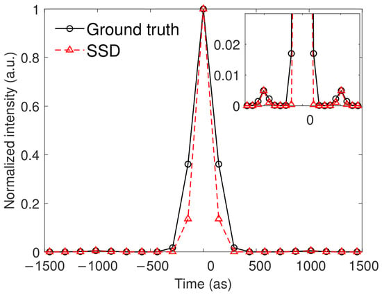
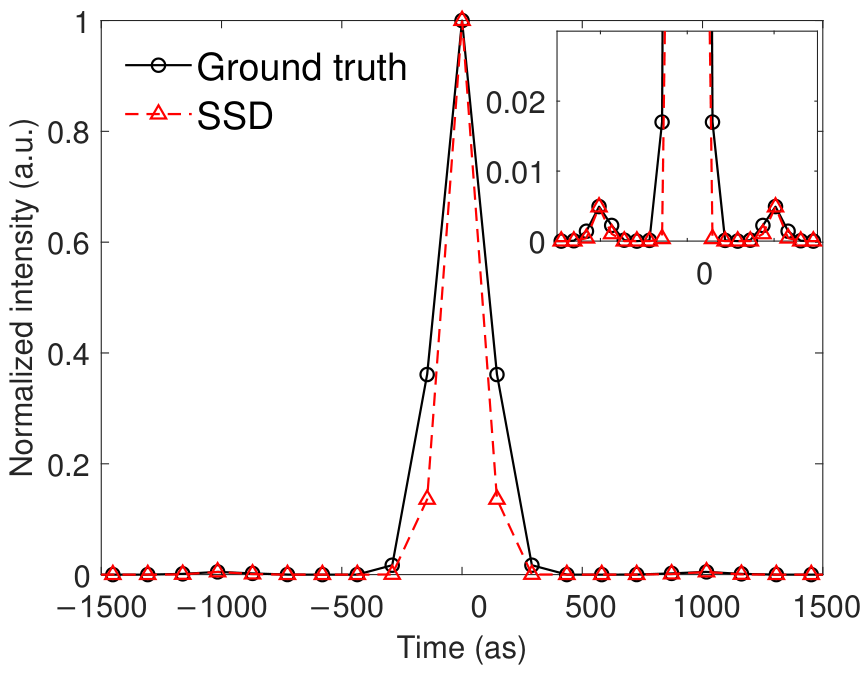
To test the capability of SSD to reconstruct nonideal pulse shapes, we simulated an attosecond pulse with two weak satellite pulses (0.5% peak intensity) separated by 1000 from the main pulse. As shown in Figure 4, SSD correctly recovers both the main pulse and the weak satellite pulses. This demonstrates that TV/NLM regularization does not artificially suppress weak but real structures. Specifically, we tested a range of TV and NLM regularization weights ($k_1$ and $k_2$ from 0.01 to 1.0) and monitored both the RMSE of the reconstructed pulse (against the ground truth) and the ability to recover weak satellite pulses (0.5% intensity). The results show that: (1) When both $k_1$ and $k_2$ are below 0.05, the reconstruction is sensitive to noise, and the satellite pulses are obscured by noise artifacts. (2) When $k_1$ and $k_2$ are in the range of 0.05–0.5, both noise suppression and satellite pulse preservation are achieved. (3) When $k_1$ and $k_2$ exceed 1.0, the regularization over-smooths the pulse, and the satellite pulses are suppressed. The optimal range (0.05–0.5) is relatively wide, indicating that the method is not overly sensitive to the regularization parameters.

Figure 4. Reconstruction of a nonideal attosecond pulse with weak satellite pulses. Temporal intensity profile showing main pulse and satellite pulses (0.5% peak intensity).

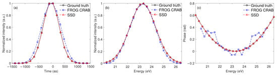
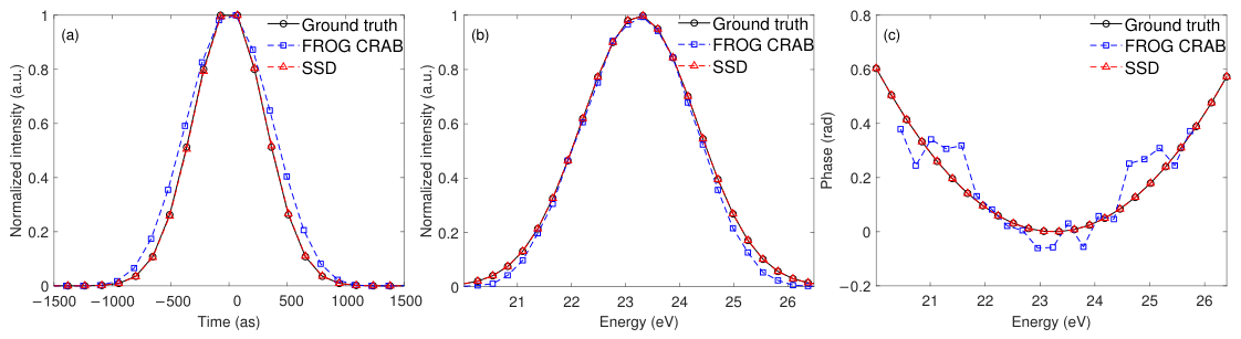
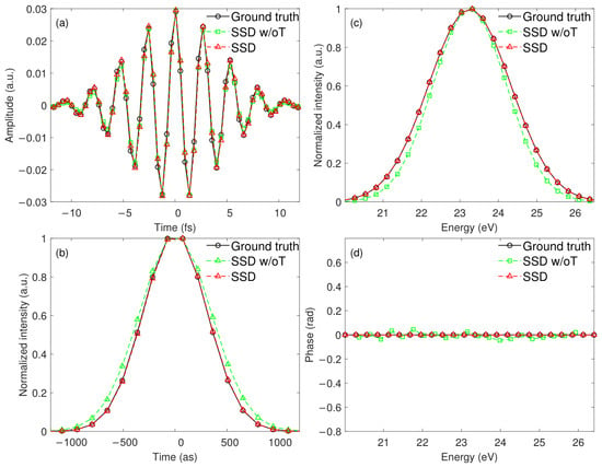
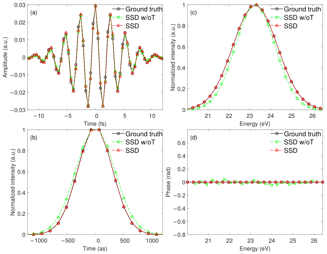
To validate the phase retrieval capability for pulses with nontrivial spectral phase, we simulated an attosecond pulse with significant group delay dispersion (GDD). As shown in Figure 5, SSD correctly retrieves the nontrivial spectral phase. Under noisy conditions ($\lambda =10$), SSD maintains accurate phase retrieval, while FROG CRAB introduces significant phase errors. SSD achieved remarkably good reconstruction results using only a very small number of training samples. Even without any training—when the method performs direct inference (SSD w/oT)—it significantly outperforms FROG CRAB (see the quantitative metrics in Table 1 and Table 2), demonstrating the overall superiority of self-supervised deep learning algorithms. Indeed, training with a small number of samples enables the entire network framework to perform inference faster and more accurately (as shown in Figure 6 and as evidenced by the quantitative metrics in Table 1 and Table 2).

Figure 5. Reconstruction of attosecond pulse with nontrivial spectral phase. (a) Temporal intensity profile. (b) Spectral intensity distribution. (c) Spectral phase distribution showing significant GDD. Results obtained by FROG CRAB and SSD are compared with ground truth.

Figure 6. Comparison of reconstruction results between self-supervised deep learning algorithm with direct inference without training (SSD w/oT) and training-and-inference approach (SSD). The input is a simulated attosecond streaking spectrogram corrupted by Poisson noise ($\lambda =5$). (a) Comparison of femtosecond pulses. (b–d) Characterization of attosecond pulses: (b) temporal intensity profile, (c) spectral intensity distribution, and (d) spectral phase distribution. Results obtained by SSD w/oT and SSD are compared with ground truth.

We used cosine similarity (CS) and root mean square error (RMSE) to quantitatively evaluate the reconstruction results. CS assessed the recovery of the light pulse profile, while RMSE measured the absolute amplitude error between the retrieved pulse and the ground truth at each sampling point. Table 1 shows a comparison of the CS metric for the retrieval of attosecond and femtosecond pulses using three methods: FROG CRAB, SSD w/oT, and SSD. Under low-energy conditions without noise, the CS values for all three methods were greater than 0.98, indicating that the retrieved pulses closely matched the ground truth, and the retrieved profiles were excellent. As the noise level increased, the reconstruction performance of FROG CRAB deteriorated progressively, with distortions appearing in the fine details of the pulse profile and rendering the retrieved phase of the attosecond pulse unreliable. In contrast, the reconstruction performance of SSD remained nearly unaffected, demonstrating the high precision of the network model in physically modeling the attosecond time-resolved photoelectron spectrogram and its strong robustness against noise. Even for SSD w/oT, the reconstruction performance is only slightly affected by noise. At higher energies, under the same noise conditions, the reconstruction performance of all methods improves to some extent.

For femtosecond infrared pulses, we also compared the RMSE of the reconstruction results obtained using various methods. As shown in Table 2, the RMSE values of the reconstruction results from the different methods exhibited trends similar to those observed for the CS metric. Under low-energy conditions (9.65 eV), from the case without noise to the case with severe Poisson noise ($\lambda =5$), the RMSE values of the reconstruction results obtained by FROG CRAB, SSD w/oT, and SSD increased by factors of 4.17, 2.38, and 1.53, respectively. Under high-energy conditions (49.95 eV), the corresponding RMSE values increased by factors of 3.41, 2.23, and 1.80, respectively.

We note that the reconstruction accuracy depends only weakly on the number of training spectrograms. Because the primary reconstruction capability originates from the physical constraints in the differentiable model rather than from the training data, even direct inference without prior training yields reasonable reconstructions. The addition of a small number of training samples further refines the network’s initialization, but the improvement quickly saturates, confirming that the method requires only a very small number of training samples. This is a key advantage of the self-supervised approach over supervised methods that typically require large datasets.

3.3. Reconstruction Results from Experimental Measurements

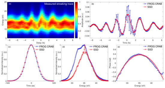
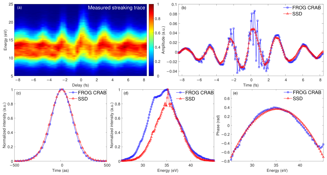
Figure 7a shows the attosecond streaking spectrogram of neon atoms obtained experimentally. To provide an objective measure of reconstruction quality, we computed the root mean square residual between the measured spectrogram and the spectrogram forward-calculated using the retrieved XUV and IR fields. The residual for SSD is 8.7% of the peak signal, compared to 14.2% for FROG CRAB, indicating that the SSD reconstruction provides a more consistent fit of the experimental data. We note that the FROG CRAB reconstruction was performed using the standard VTGPA algorithm. A more carefully optimized FROG CRAB reconstruction could yield improved results, and the present comparison should not be interpreted as a definitive benchmark but rather as an illustration of the relative performance under equivalent algorithmic settings. Figure 7b displays the retrieved femtosecond pulses using FROG CRAB and SSD. Near the center of the pulses, the FROG CRAB results exhibit severe random fluctuations, with the amplitude of these fluctuations even exceeding the pulse amplitude. In contrast, the SSD results provide a more consistent fit to the measured spectrogram, as confirmed by the quantitative residual analysis (RMS residual: 8.7% for SSD vs. 14.2% for FROG CRAB). We note that while the TV and NLM regularization in SSD explicitly encourages smoothness, the lower residual indicates better data consistency. The FROG CRAB reconstruction exhibits unphysical amplitude fluctuations (with fluctuation amplitude exceeding the pulse amplitude), which are attributed to noise-induced instability rather than the preservation of real structures. Figure 7c–e present the reconstruction results of the attosecond pulses. The narrower pulse width and broader spectral bandwidth of the FROG CRAB reconstruction can be attributed to the noise amplification in the iterative optimization, which tends to create spurious high-frequency components. The random fluctuations in the SSD-retrieved XUV spectrum are likely due to model mismatch between the SFA forward model and the experimental data.

Figure 7. Comparison of reconstruction results between FROG CRAB and SSD. (a) Input data were experimentally measured attosecond streaking spectrogram of neon atoms [20]. (b) Comparison of femtosecond pulses. (c–e) Characterization of attosecond pulses: (c) temporal intensity profile, (d) spectral intensity distribution, and (e) spectral phase distribution.

4. Conclusions and Outlook

This paper addresses the challenging problem of collaboratively retrieving attosecond XUV and femtosecond infrared pulses by introducing a self-supervised deep learning reconstruction algorithm that incorporates physical constraints. The algorithm abandons the traditional central momentum approximation and leverages position-encoded MLP and Fourier feature projection, effectively enhancing the network’s ability to capture high-frequency temporal details in ultrashort pulses. By constructing a physics-based differentiable model, we establish a self-supervised training pipeline that requires no paired labeled data, thereby overcoming the bottleneck due to scarce attosecond experimental samples. The training process is concise and highly physically interpretable. Dynamic masking and noise injection strategies significantly improve the model’s robustness against interference, enabling it to maintain high accuracy even under low signal-to-noise ratio conditions. A detail optimization module that integrates total variation and non-local mean priors constrains the shape of the light field from both local and global perspectives, greatly enhancing the geometric consistency of the retrieved pulses. Both qualitative and quantitative tests validate the effectiveness of this approach, demonstrating that the proposed framework can simultaneously achieve high-precision co-reconstruction of femtosecond infrared and attosecond XUV pulses.

We note that the current implementation uses the SFA model for both data generation and the differentiable physical model. In future work, more sophisticated forward models incorporating energy-dependent dipole matrix elements and Coulomb effects will be explored to further reduce the model mismatch for experimental data. The current framework does not explicitly account for several systematic experimental nonidealities, including the finite energy resolution of the electron spectrometer and spatial/volume averaging effects [30,31]. These effects can be incorporated into the differentiable physical model by convolving the simulated spectrogram with the instrument response function and by integrating over the interaction volume, respectively. Future work will focus on implementing these extensions to further bridge the gap between simulation and experiment.

This study deeply integrates self-supervised deep learning with an ultrafast photoionization physical model to synergistically retrieve of two different types of ultrashort pulses. It expands the applicability of the attosecond photoelectron spectrogram reconstruction algorithms and provides a new, intelligent technological solution for attosecond metrology and ultrafast spectral analysis. This approach holds promise for further advancing the application of deep learning in the field of extreme ultrafast optics.

References

- Krausz, F.; Ivanov, M. Attosecond physics. Rev. Mod. Phys. 2009, 81, 163–234. [Google Scholar] [CrossRef] [Scilit]
- Goulielmakis, E.; Loh, Z.H.; Wirth, A.; Santra, R.; Rohringer, N.; Yakovlev, V.S.; Zherebtsov, S.; Pfeifer, T.; Azzeer, A.M.; Kling, M.F.; et al. Real-time observation of valence electron motion. Nature 2010, 466, 739–743. [Google Scholar] [CrossRef] [Scilit] [PubMed]
- Zhao, K.; Gao, Y.-T.; Zhu, X.-X.; Xu, S.-Y.; Jiang, Y.-J.; Li, Y.-F.; Wang, J.; Zhu, J.-F.; Zhang, D.; Chen, Y.-L.; et al. Principle and technology of attosecond pulse characterization. Chin. Sci. Bull. 2021, 66, 835–846. [Google Scholar] [CrossRef] [Scilit]
- Chini, M.; Zhao, K.; Chang, Z. The generation, characterization and applications of broadband isolated attosecond pulses. Nat. Photon. 2014, 8, 178–186. [Google Scholar] [CrossRef] [Scilit]
- Cousin, S.L.; Di Palo, N.; Buades, B.; Teichmann, S.M.; Reduzzi, M.; Devetta, M.; Kheifets, A.; Sansone, G.; Biegert, J. Attosecond streaking in the water window: A new regime of attosecond pulse characterization. Phys. Rev. X 2017, 7, 041030. [Google Scholar] [CrossRef] [Scilit]
- Gaumnitz, T.; Jain, A.; Pertot, Y.; Huppert, M.; Jordan, I.; Ardana-Lamas, F.; Wörner, H.J. Streaking of 43-attosecond soft-X-ray pulses generated by a passively CEP-stable mid-infrared driver. Opt. Express 2017, 25, 27506–27518. [Google Scholar] [CrossRef] [Scilit] [PubMed]
- Witting, T.; Osolodkov, M.; Schell, F.; Morales, F.; Patchkovskii, S.; Šušnjar, P.; Cavalcante, F.H.M.; Menoni, C.S.; Schulz, C.P.; Furch, F.J.; et al. Generation and characterization of isolated attosecond pulses at 100 kHz repetition rate. Optica 2022, 9, 145–151. [Google Scholar] [CrossRef] [Scilit]
- Witting, T.; Furch, F.J.A.J.; Kornilov, O.; Osolodkov, M.; Schulz, C.P.; Vrakking, M.J.J. Retrieval of attosecond pulse ensembles from streaking experiments using mixed state time-domain ptychography. J. Phys. B At. Mol. Opt. Phys. 2020, 53, 194001. [Google Scholar] [CrossRef] [Scilit]
- Brunner, C.; Duensing, A.; Schroeder, C.; Mittermair, M.; Golkov, V.; Pollanka, M.; Cremers, D.; Kienberger, R. Deep learning in attosecond metrology. Opt. Express 2022, 30, 15669–15684. [Google Scholar] [CrossRef] [Scilit] [PubMed]
- Itatani, J.; Quéré, F.; Yudin, G.L. Attosecond streaking camera. Phys. Rev. Lett. 2002, 88, 173903. [Google Scholar] [CrossRef] [Scilit] [PubMed]
- Calegari, F.; Sansone, G.; Stagira, S.; Vozzi, C.; Nisoli, M. Advances in attosecond science. J. Phys. B At. Mol. Opt. Phys. 2016, 49, 062001. [Google Scholar] [CrossRef] [Scilit]
- Peng, L.Y.; Jiang, W.C.; Geng, J.W.; Xiong, W.-H.; Gong, Q. Tracing and controlling electronic dynamics in atoms and molecules by attosecond pulses. Phys. Rep. 2015, 575, 1–71. [Google Scholar] [CrossRef] [Scilit]
- Mairesse, Y.; Quéré, F. Frequency-resolved optical gating for complete reconstruction of attosecond bursts. Phys. Rev. A 2005, 71, 011401(R). [Google Scholar] [CrossRef] [Scilit]
- Zhao, K.; Zhang, Q.; Chini, M.; Wu, Y.; Wang, X.; Chang, Z. Tailoring a 67-attosecond pulse through advantageous phase-mismatch. Opt. Lett. 2012, 37, 3891. [Google Scholar] [CrossRef] [Scilit] [PubMed]
- Chini, M.; Gilbertson, S.; Khan, S.D.; Chang, Z. Characterizing ultrabroadband attosecond lasers. Opt. Express 2010, 18, 13006–13016. [Google Scholar] [CrossRef] [Scilit] [PubMed]
- Keathley, P.D.; Bhardwaj, S.; Moses, J.; Laurent, G.; Kärtner, F.X. Volkov transform generalized projection algorithm. New J. Phys. 2016, 18, 073009. [Google Scholar] [CrossRef] [Scilit]
- Zhao, X.; Wei, H.; Wu, Y.; Lin, C.D. Phase-retrieval algorithm for broadband single attosecond pulses. Phys. Rev. A 2017, 95, 043407. [Google Scholar] [CrossRef] [Scilit]
- Yu, W.W.; Zhao, X.; Wei, H.; Wang, S.-J.; Lin, C.D. Method for spectral phase retrieval of single attosecond pulses using the autocorrelation of photoelectron streaking spectra. Phys. Rev. A 2019, 99, 033403. [Google Scholar] [CrossRef] [Scilit]
- Yang, Z.; Cao, W.; Chen, X.; Zhang, J.; Mo, Y.; Xu, H.; Mi, K.; Zhang, Q.; Lan, P.; Lu, P. All-optical frequency-resolved optical gain for isolated attosecond pulse reconstruction. Opt. Lett. 2020, 45, 567–570. [Google Scholar] [CrossRef] [Scilit]
- Yang, Z.; Cao, W.; Mo, Y.; Xu, H.; Mi, K.; Lan, P.; Zhang, Q.; Lu, P. All-optical attosecond time-domain interferometry. Natl. Sci. Rev. 2021, 8, nwaa211. [Google Scholar] [CrossRef] [Scilit] [PubMed]
- White, J.; Chang, Z. Attosecond streaking phase retrieval with neural network. Opt. Express 2019, 27, 4799–4810. [Google Scholar] [CrossRef] [Scilit] [PubMed]
- Zhu, Z.; White, J.; Chang, Z.; Pang, S. Attosecond pulse retrieval from noisy streaking traces with conditional variational generative network. Sci. Rep. 2020, 10, 5782. [Google Scholar] [CrossRef] [Scilit] [PubMed]
- Zahavy, T.; Dikopoltsev, A.; Moss, D.; Haham, G.I.; Cohen, O.; Mannor, S.; Segev, M. Deep learning reconstruction of ultrashort pulses. Optica 2018, 5, 666–673. [Google Scholar] [CrossRef] [Scilit]
- Zang, G.; Idoughi, R.; Li, R.; Wonka, P.; Heidrich, W. IntraTomo: Self-supervised Learning-based Tomography via Sinogram Synthesis and Prediction. In Proceedings of the 2021 IEEE/CVF International Conference on Computer Vision (ICCV), Montreal, QC, Canada, 10–17 October 2021; pp. 1960–1970. [Google Scholar]
- Tancik, M.; Srinivasan, P.; Mildenhall, B.; Fridovich-Keil, S.; Raghavan, N.; Singhal, U.; Ramamoorthi, R.; Barron, J.T.; Ng, R. Fourier features let networks learn high frequency functions in low dimensional domains. Adv. Neural Inf. Process. Syst. 2020, 33, 7537–7547. [Google Scholar]
- Adler, J.; Kohr, H.; Oktem, O. Operator Discretization Library (ODL). Available online: https://github.com/odlgroup/odl (accessed on 11 March 2026).
- Buades, A.; Coll, B.; Morel, J.-M. A non-local algorithm for image denoising. In Proceedings of the 2005 IEEE Computer Society Conference on Computer Vision and Pattern Recognition (CVPR’05), San Diego, CA, USA, 20–25 June 2005; Volume 2, pp. 60–65. [Google Scholar]
- Lewenstein, M.; Balcou, P.; Ivanov, M.Y.; L’huillier, A.; Corkum, P.B. Theory of high-harmonic generation by low-frequency laser fields. Phys. Rev. A 1994, 49, 2117–2132. [Google Scholar] [CrossRef] [Scilit] [PubMed]
- Liu, K.; Wang, F.; Liao, Q.; Cao, W.; Lu, P.; Thumm, U. Comprehensive spatial and temporal analysis of attosecond time-resolved photoemission dynamics. Opt. Express 2026, 34, 5102–5118. [Google Scholar] [CrossRef] [Scilit] [PubMed]
- Wei, H.; Morishita, T.; Lin, C.D. Critical evaluation of attosecond time delays retrieved from photoelectron streaking measurements. Phys. Rev. A 2016, 93, 053412. [Google Scholar] [CrossRef] [Scilit]
- Vismarra, F.; Borrego-Varillas, R.; Wu, Y.; Mocci, D.; Nisoli, M.; Lucchini, M. Ensemble effects on the reconstruction of attosecond pulses and photoemission time delays. J. Phys. Photonics 2022, 4, 034006. [Google Scholar] [CrossRef] [Scilit]
Disclaimer/Publisher’s Note: The statements, opinions and data contained in all publications are solely those of the individual author(s) and contributor(s) and not of MDPI and/or the editor(s). MDPI and/or the editor(s) disclaim responsibility for any injury to people or property resulting from any ideas, methods, instructions or products referred to in the content. |
© 2026 by the authors. Licensee MDPI, Basel, Switzerland. This article is an open access article distributed under the terms and conditions of the Creative Commons Attribution (CC BY) license.