Key Physicochemical and Biological Factors Associated with Chlorophyll-a Concentrations: A Machine Learning Approach

Abstract

Chlorophyll-a is a widely used indicator for assessing the trophic status and water quality of aquatic ecosystems because of its close relationship with phytoplankton biomass. This study aimed to identify the physicochemical, biological, and temporal variables associated with chlorophyll-a concentrations in Lake Gatun during the 2017–2023 period using the Light Gradient Boosting Machine (LightGBM) algorithm and a Generalized Linear Model (GLM). A total of 25 predictor variables describing water quality were analyzed using data collected from 14 monitoring stations distributed throughout Lake Gatun within the Panama Canal watershed. The LightGBM model achieved satisfactory predictive performance, with an RMSE of 4.58, an MAE of 3.26, and a coefficient of determination (R²) of 0.42 on the testing dataset. Variable importance analysis identified turbidity, dissolved oxygen, and water transparency as the most influential predictors of chlorophyll-a concentrations. These findings improve our understanding of the factors associated with chlorophyll-a variability and demonstrate the potential of machine learning models as decision-support tools for monitoring and managing aquatic ecosystems.

1. Introduction

Freshwater lakes are dynamic ecosystems that play a fundamental role in maintaining aquatic biodiversity and regulating water quality [1]. Within these ecosystems, chlorophyll-a (Chl-a) is the primary indicator of phytoplankton biomass owing to its sensitivity to physicochemical changes and nutrient availability [2,3,4,5,6]. Chlorophyll-a is closely associated with eutrophication processes and variations in water quality [7,8,9,10]; consequently, increases in its concentration are commonly linked to nutrient enrichment, dissolved oxygen depletion, and alterations in the ecological structure of these ecosystems [11,12].

Numerous studies have shown that Chl-a concentrations are influenced by environmental factors such as temperature, pH, electrical conductivity, salinity, and nutrient availability [5,6]. These factors regulate phytoplankton growth and distribution, resulting in pronounced spatial and temporal variability in Chl-a concentrations [13,14].

In tropical ecosystems, nutrient availability—particularly nitrogen and phosphorus— plays a fundamental role in regulating phytoplankton productivity and eutrophication processes [15,16,17]. In addition, climate change may alter the structure and functioning of aquatic ecosystems through changes in water temperature and precipitation patterns [18,19]. Such changes can enhance nutrient uptake by phytoplankton, accelerating eutrophication processes and unpredictably modifying the temporal dynamics of chlorophyll-a concentrations [20].

Understanding these processes is particularly important in strategically important tropical ecosystems such as Lake Gatun, which is essential for the hydrological sustainability and operation of the Panama Canal [21]. This artificial reservoir, covering approximately 436 km², is the basin’s main freshwater storage system and supplies the water needed for ship transit through the canal, as well as drinking water for more than half of Panama’s population [22]. The lake also supports high biological diversity and contributes to regional hydrological regulation. Despite its ecological and socioeconomic importance, the relationships between environmental variables and Chl-a concentrations in Lake Gatun remain poorly understood [23]. Important knowledge gaps persist regarding the nonlinear and multidimensional interactions that govern the spatial and temporal variability, partly because machine learning approaches have rarely been applied to this ecosystem.

The identification of these processes has evolved considerably over recent decades, shifting from conventional statistical approaches to machine learning methodologies capable of modeling complex relationships among multiple environmental variables. Traditionally, studies on chlorophyll-a have focused on examining its relationship with water quality parameters and spatial distribution using conventional statistical methods, including Pearson’s correlation coefficient, simple and multiple linear regression, log-linear regression, and multivariate techniques [24,25,26,27,28,29,30]. More recently, however, machine learning algorithms have demonstrated remarkable ability to identify the factors influencing Chl-a variability and dynamics [1], while improving the prediction of Chl-a concentrations in aquatic ecosystems. Among the most widely used techniques are Random Forest [14,31,32], artificial and convolutional neural networks [33,34,35], support vector regression (SVR) [36] and Light Gradient Boosting Machine (LightGBM) [37]. Their performance has recently been compared for modeling Chl-a concentrations [8,38,39], as well as for water quality assessment and prediction [40,41] and streamflow forecasting [42].

Against this background, there is a need to incorporate analytical approaches capable of modeling nonlinear relationships and interpreting the contribution of multiple environmental variables to Chl-a dynamics. Therefore, the objective of this study was to identify the physicochemical and biological parameters exerting the greatest influence on the distribution of chlorophyll-a concentrations in Lake Gatun. To achieve this, a hybrid framework was adopted. First, the Light Gradient Boosting Machine (LightGBM) algorithm was implemented to identify the most influential predictor variables and capture complex nonlinear interactions. Subsequently, SHapley Additive exPlanations (SHAP) were used to interpret the contribution and direction of the effect of each variable on the model predictions. Finally, a Generalized Linear Model (GLM) was fitted to quantify the magnitude and statistical significance of the identified associations.

The scientific contribution of this study lies in the integration of LightGBM, SHAP, and GLM within a single analytical framework to investigate Chl-a dynamics in Lake Gatun. Unlike previous studies in this ecosystem, which have primarily focused on conventional statistical analyses [23], the proposed approach combines the predictive capability of machine learning with model interpretability and statistical inference. This integrated framework not only identifies the environmental variables driving chlorophyll-a variability but also provides an ecological interpretation of their effects, thereby extending current knowledge of the processes governing phytoplankton dynamics in this tropical reservoir.

2. Materials and Methods

This study analyzed water quality parameters measured in Lake Gatun, located within the Panama Canal watershed [43]. A set of physicochemical and biological variables was evaluated to determine their influence on Chl-a concentrations.

Lake Gatun, located in central Panama, is one of the country’s most important artificial reservoirs and the primary freshwater source supporting the operation of the Panama Canal. The lake covers an area of approximately 436 km² and lies at an average elevation of 27 m above sea level, centered at 9°12′ N and 79°54′ W. It was created by damming the Chagres River and its tributaries during the construction of the Panama Canal and currently plays a fundamental role in both ship transit and the drinking water supply for more than half of Panama’s population. The lake is characterized by a humid tropical climate with two well-defined seasons—a dry season and the rainy season—which strongly influence local hydrological patterns and water quality dynamics [44]. In addition, the lake receives inflows from numerous tributaries within the Chagres River basin, resulting in marked spatial and temporal variability in its physicochemical and biological conditions.

2.1. Data Description

The dataset consisted of monthly water quality measurements collected between January 2017 and December 2023 at 14 monitoring stations distributed throughout Lake Gatun in the Panama Canal. Each observation corresponded to a single monthly sampling event conducted at one of the 14 monitoring stations in Lake Gatun. Monthly sampling was carried out continuously from January 2017 to December 2023, resulting in 84 observations per station (12 monthly observations per year over seven years) and a total of 1176 observations. No changes in sampling frequency, laboratory analytical procedures, or data availability occurred during the study period.

The dataset comprised 24 physicochemical and biological parameters measured in the surface layer of the lake, along with a temporal variable (sampling month), collected through the Water Quality Monitoring and Surveillance Program of the Panama Canal Watershed. Laboratory analyses were conducted following the procedures described in Standard Methods for the Examination of Water and Wastewater, 23rd Edition [45].

The physicochemical and biological parameters included in the analysis are summarized in

Table 1. The physicochemical and biological water quality parameters examined in the study.

Code	Variable	Unit
Chl-a	Chlorophyll a	μg/L
TC	Total coliforms	NMP/100 mL
TDS	Total dissolved solids	mg/L
E. coli	Escherichia coli	NMP/100 mL
TSS	Total suspended solids	mg/L
Turb	Turbidity	NTU
PO4-P	Phosphorus as phosphate	mg/L
TP	Total Phosphorus	mg/L
NO2-N	Nitrogen as nitrite	mg/L
NO3-N	Nitrogen as nitrate	mg/L
Alk	Total alkalinity	mg/L
SO4	Sulfate	mg/L
Cl	Chlorides	mg/L
Na	Sodium	mg/L
Ca	Calcium	mg/L
Mg	Magnesium	mg/L
K	Potassium	mg/L
Hard	Water hardness	mg/L
Cond	Conductivity	μS/cm
Sal	Salinity	UPS
pH	Hydrogen ion potential	pH units
DO	Dissolved oxygen	mg/L
O2-Sat	Oxygen saturation percentage	%
Transp	Transparency	m
Temp	Temperature	°C

.

Chlorophyll-a concentration was defined as the response variable. A total of 25 predictor variables were considered, including 24 physicochemical and biological parameters, and sampling month as a temporal predictor. Sampling month was incorporated to account for seasonal variability, as Lake Gatun is characterized by a tropical climate with two well-defined seasons: a dry season (December–April) and a rainy season (May–November). These seasonal changes can influence hydrological conditions, nutrient transport, water transparency, turbidity, and phytoplankton dynamics. Consequently, including sampling month enabled the model to capture temporal variability that may not be fully explained by the physicochemical and biological measurements collected during each sampling event.

2.2. Methodology

In this study, a machine learning approach based on the Light Gradient Boosting Machine algorithm [46] was implemented to identify, rank and interpret the main predictor variables associated with variations in Chl-a concentrations.

Before model development, the dataset underwent a quality control and preprocessing procedure to verify its integrity, consistency, and completeness. No missing values, duplicated records, or incomplete sampling events were identified. The chronological sequence of the observations was also verified to ensure temporal consistency. Outliers were examined and retained because they were considered plausible observations representing the natural variability of the system rather than measurement errors. No imputation or data transformation procedures were applied. Likewise, no scaling or normalization was performed because LightGBM is a tree-based algorithm whose performance is not affected by differences in the scale of the predictor variables.

The dataset was chronologically divided into training (2017–2021) and testing (2022–2023) subsets to develop the model and evaluate its predictive performance on data not used during training. This temporal partitioning prevents the use of future information during model development and allows the assessment of the model’s generalization ability under a more realistic prediction scenario.

To reduce redundancy among predictors before model training, the correlation among predictor variables was assessed using Pearson’s correlation coefficient. When two or more variables exhibited an absolute correlation coefficient (|r|) greater than 0.80, only one was retained. The representative variable was selected based on its limnological relevance, prioritizing those with a more direct interpretation of the physical, chemical, or biological processes occurring within the system. This procedure was designed to reduce redundancy among predictors while preserving variables representative of the main environmental processes evaluated.

The LightGBM hyperparameters were tuned through a manual tuning procedure by evaluating different combinations of the main model parameters (num_leaves, max_depth, learning_rate, lambda_l2 and feature_fraction). The final hyperparameter values were selected based on predictive performance, assessed using RMSE on the validation dataset, while also considering model complexity to reduce the risk of overfitting.

The model was subsequently trained and evaluated using regression performance metrics to assess its predictive ability and identify the most relevant predictors associated with Chl-a concentration. Next, the contribution of each predictor variable to model performance was assessed using SHapley Additive exPlanations [47,48], an artificial intelligence-based interpretability technique that ranks variable importance and quantifies both the direction and magnitude of each variable’s contribution to the model predictions.

Finally, to complement the interpretation of the machine learning approach, the variables with the highest predictive importance were incorporated into a Generalized Linear Model (GLM) [49,50] to quantify the magnitude and statistical significance of their associations with Chl-a concentrations [51].

2.2.1. LightGBM

LightGBM belongs to the family of gradient boosting algorithms [46], in which the final prediction is generated through the sequential combination of multiple decision trees [52]. Unlike traditional gradient boosting approaches that grow trees level by level, LightGBM adopts a leaf-wise tree growth strategy, enabling faster convergence and greater predictive accuracy. In addition, LightGBM incorporates two techniques that improve computational efficiency: Gradient-based One-Side Sampling (GOSS), which reduces the number of observations used during training by prioritizing samples with large gradients, and Exclusive Feature Bundling (EFB), which reduces data dimensionality by grouping mutually exclusive features.

Mathematically, the prediction of the model can be expressed as the sum of the individual trees forming the ensemble:

$$F_M\left(x\right)={\displaystyle \sum _{m=1}^M}{\gamma }_m{h}_m\left(x\right)$$

where $F_M\left(x\right)$ denotes the final model prediction, $h_m(x)$ represents the m-th decision tree, and ${\gamma }_m$ is the weight associated with the contribution of each tree. Through an iterative learning process, each new tree is fitted to the residual errors of the previously constructed trees, progressively improving prediction accuracy.

Although the learning mechanism is defined by the algorithm’s structure, the predictive performance of LightGBM largely depends on the appropriate selection of its hyperparameters, which control model complexity, learning speed, and the tree construction process. The main hyperparameters optimized in this study are presented in

Table 2. The main parameters of LightGBM.

Parameter	Description
num_leaves	This is the number of leaves per tree.
max_depth	This describes the maximum depth of the tree.
learning_rate	This controls the speed of iteration.
lambda_l2	This is the L2 regularization parameter that reduces overfitting.
feature_fraction	This is the fraction of features selected randomly in each iteration for building trees.

.

One of the main reasons for selecting LightGBM in the present study is its ability to efficiently model complex nonlinear relationships and interactions among environmental variables while maintaining high predictive performance and computational efficiency. Compared with other tree-based ensemble methods, LightGBM uses a leaf-wise tree growth strategy together with Gradient-based One-Side Sampling (GOSS), allowing faster training and efficient handling of high-dimensional datasets. In addition, as a tree-based gradient boosting algorithm, it does not require the predictor variables to satisfy strict statistical assumptions such as normality, homoscedasticity, or linear relationships with the response variable [53]. This characteristic makes it particularly suitable for the analysis of aquatic ecosystems, where physicochemical and biological parameters often exhibit skewed distributions, extreme values, and complex nonlinear interactions. Consequently, LightGBM can efficiently model these relationships without requiring prior data transformations to satisfy parametric assumptions, thereby facilitating pattern detection and the identification of the factors most strongly associated with chlorophyll-a concentrations.

2.2.2. SHapley Additive exPlanations (SHAP)

In machine learning, interpretability is a fundamental aspect of understanding how predictor variables contribute to the model predictions. SHAP is an explainable artificial intelligence (XAI) method based on Shapley values from cooperative game theory that estimates the marginal contribution of each predictor variable to those model predictions [47].

To estimate this contribution, SHAP computes the average effect of adding a variable to the model across all possible combinations of predictor variables. Mathematically, the SHAP value ${\varphi }_i\left(x\right)$ for each feature is computed by combining conditional expectations with the classical Shapley values from cooperative game theory:

$${\varphi }_i\left(x\right)=\sum _{S\subseteq F\setminus \left\{i\right\}}{\displaystyle \frac{\left|S\right|!\left(\left|F\right|-\left|S\right|-1\right)! }{\left|F\right|!}}[f(S\cup \{i\})-f(S)]$$

where ${\varphi }_i\left(x\right)$ denotes the Shapley value of feature $i$ for sample $x$, $F$ is the set of all input features, $S$ is a subset of features, and $f$ represents the model prediction.

Thus, SHAP makes it possible to identify both the relative importance of the predictor variables and the direction and magnitude of their effects on the model predictions, providing a clear and consistent interpretation of the model’s decision-making process.

2.2.3. Generalized Linear Model (GLM)

Generalized Linear Models (GLMs) are an extension of classical linear regression, allowing the relationship between a response variable and a set of predictor variables to be modeled through an appropriate probability distribution and link function [54]. A GLM relates the expected value of the response variable to a linear combination of the predictor variables while preserving the natural scale of the data. In addition to estimating the effect of each predictor, GLMs provide measures of statistical significance and the precision of the estimated coefficients. In general, a GLM can be expressed as:

$$g({\mu }_i)={\beta }_0+{\displaystyle \sum _{j=1}^p}{\beta }_j{x}_{ij}$$

where $g(({\mu }_i)$ is the link function, ${\mu }_i=E(Y_i)$ is the expected value of the response variable, ${\beta }_0$ is the intercept, and ${\beta }_j$ represents the regression coefficients associated with the predictor variables $x_{ij}$.

In this study, the GLM was used as a complementary analysis to the LightGBM model to statistically validate the variables previously identified as the most relevant and to quantify the magnitude of their associations with chlorophyll-a concentrations.

Because Chl-a concentration is a continuous, strictly positive, and right-skewed variable, a Gamma distribution with a logarithmic link function was adopted, providing an appropriate framework for modeling its distribution without assuming normality.

Overall, the proposed framework combined the strengths of three complementary approaches. LightGBM was used to model complex nonlinear relationships and estimate the relative importance of each physicochemical, biological, and temporal predictor. Based on the variable importance estimated by SHAP were applied to interpret the relative contribution of each predictor and the direction of its effect on chlorophyll-a predictions. Finally, the most relevant variables were incorporated into a GLM to quantify the magnitude and statistical significance of their associations with chlorophyll-a concentrations. This hybrid framework integrates the predictive power of machine learning for modeling nonlinear relationships with the rigor and interpretability of classical statistical inference.

All data processing and statistical analyses were performed using the R programming language through the RStudio integrated development environment, version 4.2.1 [55].

3. Results

3.1. Descriptive Statistics

Table 3. Descriptive statistics of the input variables.

Parameter	Minimum	Maximum	Mean	Standard Deviation
Chlorophyll-a	0.50	74.30	6.98	5.73
Total coliforms	5.00	160,000.00	2246.53	7229.71
Total dissolved solids	7.00	1419.00	196.80	132.06
Escherichia coli	5.00	4100.00	35.44	146.44
Total suspended solids	<10	53.00	2.76	4.57
Turbidity	0.40	90.80	3.86	6.86
Phosphorus as phosphate	<0.01	0.05	0.01	0.01
Total Phosphorus	<0.01	0.07	0.01	0.01
Nitrogen as nitrite	<0.01	0.02	<0.01	<0.01
Nitrogen as nitrate	<0.01	0.50	0.12	0.12
Total alkalinity	12.00	76.00	34.85	13.16
Sulfate	0.20	58.20	12.73	8.34
Chlorides	2.60	362.00	70.81	59.65
Sodium	0.71	251.90	40.68	32.71
Calcium	0.14	55.77	8.58	5.19
Magnesium	0.95	35.74	6.63	3.95
Potassium	0.34	10.08	2.48	1.25
Water hardness	5.90	223.00	49.21	26.55
Conductivity	42.00	1777.00	333.14	227.12
Salinity	0.01	0.89	0.16	0.12
Hydrogen ion potential	6.05	8.78	7.42	0.41
Dissolved oxygen	<0.01	9.51	6.91	0.94
Oxygen saturation percentage	<0.01	127.00	90.63	12.62
Transparency	0.10	5.00	2.24	0.98
Temperature	21.50	32.80	29.44	1.03

presents the descriptive statistics of the predictor variables, providing an overview of their distribution and variability prior to model development.

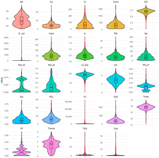
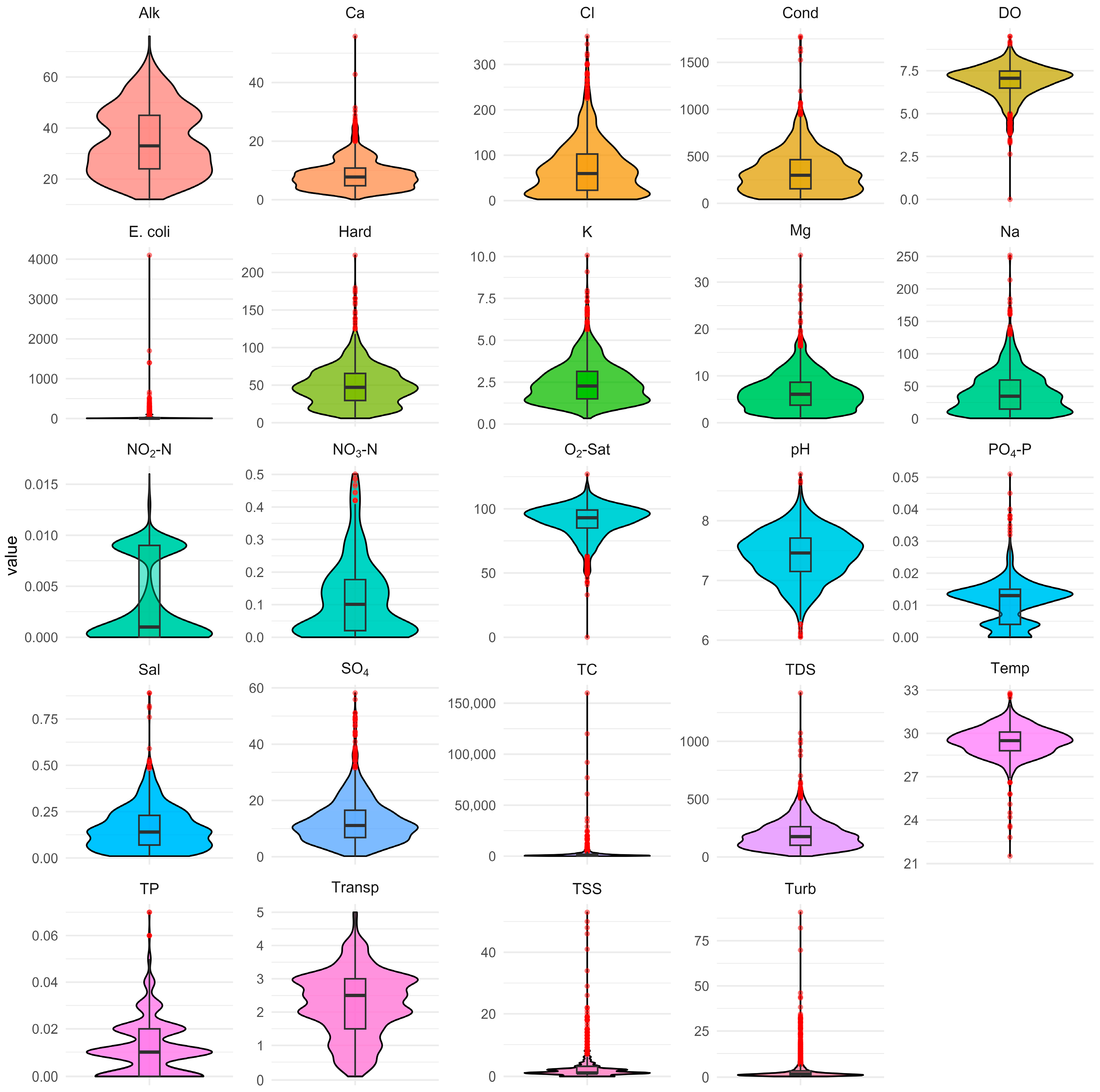
Figure 1 illustrates the distribution of the physicochemical and biological parameters using violin plots complemented by box plots.

Overall, considerable heterogeneity was observed among the variables, reflecting the complexity of the processes regulating water quality in the ecosystem. While some variables exhibited relatively stable distributions concentrated around their central values, others showed pronounced positive skewness, high dispersion, and numerous extreme values, indicating substantial spatial and temporal variability.

Variables associated with the basic physicochemical conditions of the system, including temperature (Temp), pH, dissolved oxygen (DO), and oxygen saturation (O₂-Sat), exhibited compact and nearly symmetric distributions with few outliers, suggesting relatively stable environmental conditions throughout the study period.

Variables associated with the ionic composition and mineralization of the water, including alkalinity (Alk), hardness (Hard), calcium (Ca), magnesium (Mg), sodium (Na), potassium (K), and sulfate (SO₄), generally exhibited distributions concentrated around their central values, albeit with varying levels of dispersion and skewness. In contrast, the nutrient variables (NO₃-N, NO₂-N, PO₄-P, and TP) showed pronounced positive skewness, characterized by a predominance of low values and long tails toward higher concentrations, indicating occasional increases associated with specific environmental and hydrological conditions. Likewise, microbiological variables and those related to particulate matter transport, such as total coliforms (TC), E. coli, total suspended solids (TSS) and turbidity, exhibited the greatest variability and the largest number of extreme values, reflecting localized runoff events and inputs of sediments and organic matter into the system.

Overall, the results revealed marked heterogeneity in the distributions of the analyzed variables, with a predominance of positive skewness, extreme values, and varying levels of dispersion. These characteristics reflect the dynamic nature of the physical, chemical, and biological processes regulating water quality in Lake Gatun and support the use of tree-based machine learning algorithms, such as LightGBM, which can model complex nonlinear relationships without requiring strict assumptions of normality or homoscedasticity.

3.2. Correlation Analysis

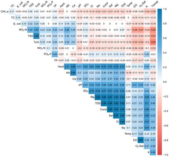
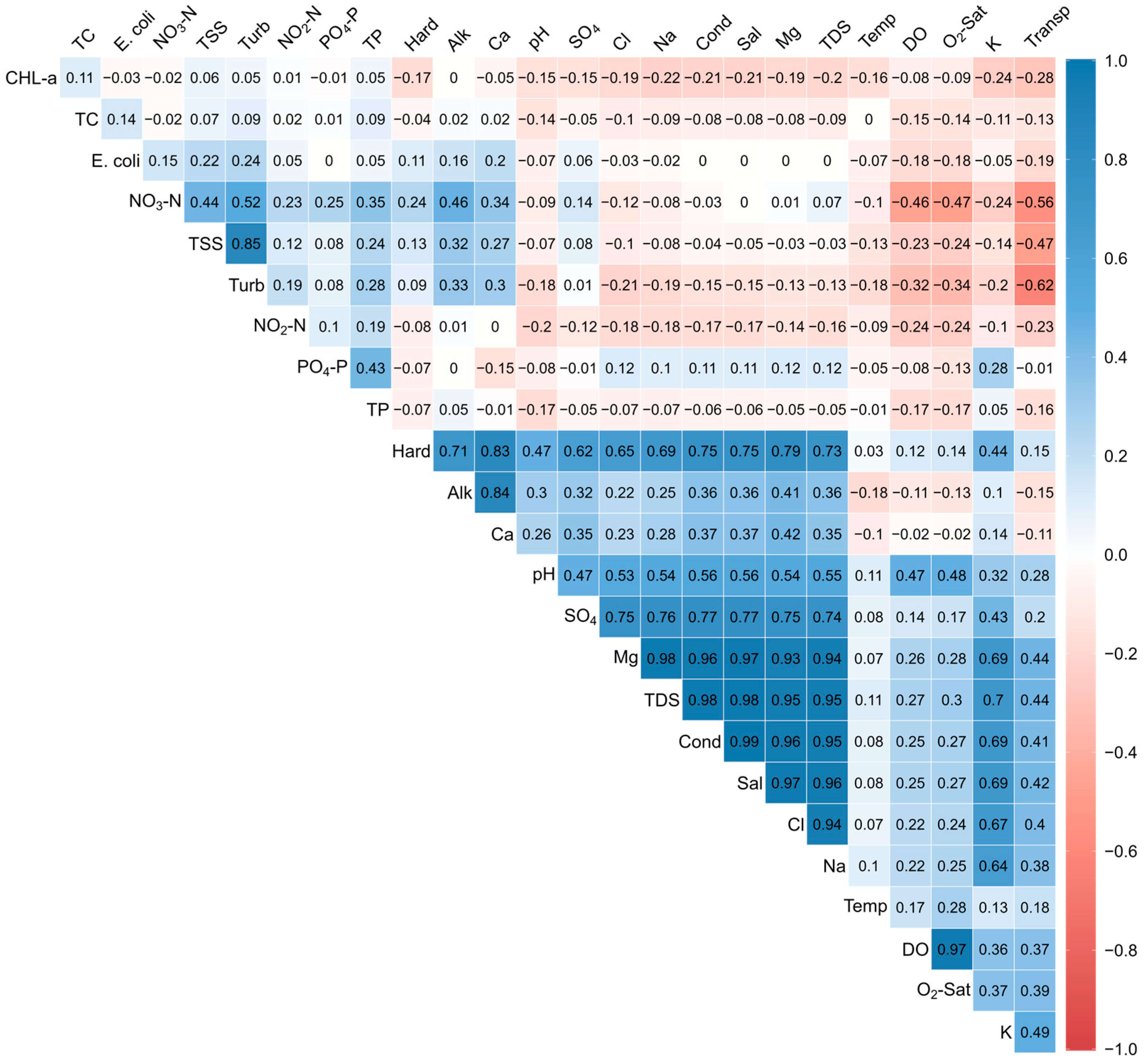
Figure 2 shows the Pearson correlation matrix between Chl-a concentrations and the predictor variables analyzed.

In general, variables associated with nutrients and suspended matter exhibited weak-to-moderate correlations with most of the analyzed parameters. However, nitrate (NO₃-N) showed moderate correlations with total coliforms (TC), E. coli, hardness (Hard), and orthophosphate (PO₄-P), indicating distinct association patterns within the set of variables analyzed. Likewise, total suspended solids (TSS) exhibited a strong positive correlation with total coliforms (TC) (r = 0.85), suggesting a close relationship between particulate matter and microbiological indicators.

Negative correlations were also observed between variables exhibiting opposite behavior, most notably between turbidity (Turb) and transparency (Transp) (r = −0.62). This relationship suggests that increases in suspended particles reduce light penetration and, consequently, water transparency. For chlorophyll-a, the observed correlations were predominantly weak, with transparency (r = −0.28) and potassium (K) (r = −0.24) showing the strongest negative associations. Negative correlations were also observed with several indicators of water mineralization, including sodium (Na), electrical conductivity (Cond), salinity (Sal), total dissolved solids (TDS), and chloride (Cl).

Overall, these results suggest that variability in Chl-a concentrations is associated with multiple environmental factors and that the relationships among these variables may involve more complex patterns that cannot be fully captured by bivariate correlation analysis.

Overall, variables associated with nutrients and suspended matter exhibited low to moderate correlations with most of the measured characteristics. However, strong correlations were observed among some variables describing similar physicochemical processes. In particular, total suspended solids (TSS) showed a strong positive correlation with total coliforms (TC) (r = 0.85), whereas turbidity was negatively correlated with water transparency (Transp) (r = −0.62), indicating that increasing concentrations of suspended particles reduce light penetration and, consequently, water transparency.

For chlorophyll-a, the observed correlations were generally weak. Water transparency (r = −0.28) and potassium (r = −0.24) exhibited the strongest negative associations. Negative correlations were also observed with several indicators of water mineralization, including sodium, electrical conductivity, salinity, total dissolved solids, and chloride.

These findings indicate that the linear associations between Chl-a and the analyzed variables were generally weak, suggesting that a substantial proportion of the variability in Chl-a concentration may be driven by nonlinear relationships or interactions among multiple environmental factors. Spearman’s rank correlations were additionally computed for comparison with the Pearson correlations, showing generally consistent association patterns; the complete Pearson and Spearman correlation matrices are provided in Appendix A (

Table A1. Pearson correlation coefficients.

	Chl_a	Alk	Ca	Cl	Cond	TC	Hard	E. coli	K	Mg	NO2−N	NO3−N	Na	DO	O2−Sat	PO4−P	pH	TP	Sal	SO4	TDS	TSS	Temp	Transp	Turb
Chl_a	1	0.00	−0.05	−0.19	−0.21	0.11	−0.17	−0.03	−0.24	−0.19	0.01	−0.02	−0.22	−0.08	−0.09	−0.01	−0.15	0.05	−0.21	−0.15	−0.20	0.06	−0.16	−0.28	0.05
Alk	0.00	1	0.84	0.22	0.36	0.02	0.71	0.16	0.10	0.41	0.01	0.46	0.25	−0.11	−0.13	0.00	0.30	0.05	0.36	0.32	0.36	0.32	−0.18	−0.15	0.33
Ca	−0.05	0.84	1	0.23	0.37	0.02	0.83	0.20	0.14	0.42	0.00	0.34	0.28	−0.02	−0.02	−0.15	0.26	−0.01	0.37	0.35	0.35	0.27	−0.10	−0.11	0.30
Cl	−0.19	0.22	0.23	1	0.96	−0.10	0.65	−0.03	0.69	0.93	−0.18	−0.12	0.98	0.26	0.28	0.12	0.53	−0.07	0.97	0.75	0.94	−0.10	0.07	0.44	−0.21
Cond	−0.21	0.36	0.37	0.96	1	−0.08	0.75	0.00	0.69	0.96	−0.17	−0.03	0.98	0.25	0.27	0.11	0.56	−0.06	0.99	0.77	0.95	−0.04	0.08	0.41	−0.15
TC	0.11	0.02	0.02	−0.10	−0.08	1	−0.04	0.14	−0.11	−0.08	0.02	−0.02	−0.09	−0.15	−0.14	0.01	−0.14	0.09	−0.08	−0.05	−0.09	0.07	0.00	−0.13	0.09
Hard	−0.17	0.71	0.83	0.65	0.75	−0.04	1	0.11	0.44	0.79	−0.08	0.24	0.69	0.12	0.14	−0.07	0.47	−0.07	0.75	0.62	0.73	0.13	0.03	0.15	0.09
E. coli	−0.03	0.16	0.20	−0.03	0.00	0.14	0.11	1	−0.05	0.00	0.05	0.15	−0.02	−0.18	−0.18	0.00	−0.07	0.05	0.00	0.06	0.00	0.22	−0.07	−0.19	0.24
K	−0.24	0.10	0.14	0.69	0.69	−0.11	0.44	−0.05	1	0.67	−0.10	−0.24	0.70	0.36	0.37	0.28	0.32	0.05	0.69	0.43	0.64	−0.14	0.13	0.49	−0.20
Mg	−0.19	0.41	0.42	0.93	0.96	−0.08	0.79	0.00	0.67	1	−0.14	0.01	0.95	0.22	0.24	0.12	0.54	−0.05	0.97	0.75	0.94	−0.03	0.07	0.40	−0.13
NO2−N	0.01	0.01	0.00	−0.18	−0.17	0.02	−0.08	0.05	−0.10	−0.14	1	0.23	−0.18	−0.24	−0.24	0.10	−0.20	0.19	−0.17	−0.12	−0.16	0.12	−0.09	−0.23	0.19
NO3−N	−0.02	0.46	0.34	−0.12	−0.03	−0.02	0.24	0.15	−0.24	0.01	0.23	1	−0.08	−0.46	−0.47	0.25	−0.09	0.35	0.00	0.14	0.07	0.44	−0.10	−0.56	0.52
Na	−0.22	0.25	0.28	0.98	0.98	−0.09	0.69	−0.02	0.70	0.95	−0.18	−0.08	1	0.27	0.30	0.10	0.54	−0.07	0.98	0.76	0.95	−0.08	0.11	0.44	−0.19
DO	−0.08	−0.11	−0.02	0.26	0.25	−0.15	0.12	−0.18	0.36	0.22	−0.24	−0.46	0.27	1	0.97	−0.08	0.47	−0.17	0.25	0.14	0.22	−0.23	0.17	0.37	−0.32
O2−Sat	−0.09	−0.13	−0.02	0.28	0.27	−0.14	0.14	−0.18	0.37	0.24	−0.24	−0.47	0.30	0.97	1	−0.13	0.48	−0.17	0.27	0.17	0.25	−0.24	0.28	0.39	−0.34
PO4−P	−0.01	0.00	−0.15	0.12	0.11	0.01	−0.07	0.00	0.28	0.12	0.10	0.25	0.10	−0.08	−0.13	1	−0.08	0.43	0.11	−0.01	0.12	0.08	−0.05	−0.01	0.08
pH	−0.15	0.30	0.26	0.53	0.56	−0.14	0.47	−0.07	0.32	0.54	−0.20	−0.09	0.54	0.47	0.48	−0.08	1	−0.17	0.56	0.47	0.55	−0.07	0.11	0.28	−0.18
TP	0.05	0.05	−0.01	−0.07	−0.06	0.09	−0.07	0.05	0.05	−0.05	0.19	0.35	−0.07	−0.17	−0.17	0.43	−0.17	1	−0.06	−0.05	−0.05	0.24	−0.01	−0.16	0.28
Sal	−0.21	0.36	0.37	0.97	0.99	−0.08	0.75	0.00	0.69	0.97	−0.17	0.00	0.98	0.25	0.27	0.11	0.56	−0.06	1	0.77	0.96	−0.05	0.08	0.42	−0.15
SO4	−0.15	0.32	0.35	0.75	0.77	−0.05	0.62	0.06	0.43	0.75	−0.12	0.14	0.76	0.14	0.17	−0.01	0.47	−0.05	0.77	1	0.74	0.08	0.08	0.20	0.01
TDS	−0.20	0.36	0.35	0.94	0.95	−0.09	0.73	0.00	0.64	0.94	−0.16	0.07	0.95	0.22	0.25	0.12	0.55	−0.05	0.96	0.74	1	−0.03	0.10	0.38	−0.13
TSS	0.06	0.32	0.27	−0.10	−0.04	0.07	0.13	0.22	−0.14	−0.03	0.12	0.44	−0.08	−0.23	−0.24	0.08	−0.07	0.24	−0.05	0.08	−0.03	1	−0.13	−0.47	0.85
Temp	−0.16	−0.18	−0.10	0.07	0.08	0.00	0.03	−0.07	0.13	0.07	−0.09	−0.10	0.11	0.17	0.28	−0.05	0.11	−0.01	0.08	0.08	0.10	−0.13	1	0.18	−0.18
Transp	−0.28	−0.15	−0.11	0.44	0.41	−0.13	0.15	−0.19	0.49	0.40	−0.23	−0.56	0.44	0.37	0.39	−0.01	0.28	−0.16	0.42	0.20	0.38	−0.47	0.18	1	−0.62
Turb	0.05	0.33	0.30	−0.21	−0.15	0.09	0.09	0.24	−0.20	−0.13	0.19	0.52	−0.19	−0.32	−0.34	0.08	−0.18	0.28	−0.15	0.01	−0.13	0.85	−0.18	−0.62	1

and

Table A2. Spearman correlation coefficients.

	Chl_a	Alk	Ca	Cl	Cond	TC	Hard	E. coli	K	Mg	NO2−N	NO3−N	Na	DO	O2−Sat	PO4−P	pH	TP	Sal	SO4	TDS	TSS	Temp	Transp	Turb
Chl_a	1	−0.08	−0.09	−0.25	−0.27	0.20	−0.21	0.12	−0.27	−0.25	0.04	−0.04	−0.28	−0.10	−0.11	−0.05	−0.20	0.09	−0.27	−0.21	−0.26	0.20	−0.12	−0.23	0.23
Alk	−0.08	1	0.90	0.37	0.50	0.12	0.74	0.19	0.18	0.53	−0.08	0.56	0.39	−0.04	−0.05	0.02	0.31	0.00	0.50	0.45	0.49	0.11	−0.20	−0.02	0.01
Ca	−0.09	0.90	1	0.43	0.55	0.12	0.86	0.16	0.25	0.59	−0.12	0.47	0.47	0.07	0.07	−0.05	0.32	−0.05	0.55	0.52	0.54	0.05	−0.10	0.04	−0.07
Cl	−0.25	0.37	0.43	1	0.96	−0.19	0.75	−0.16	0.75	0.93	−0.41	−0.17	0.98	0.35	0.37	0.07	0.57	−0.09	0.97	0.77	0.95	−0.29	0.16	0.56	−0.65
Cond	−0.27	0.50	0.55	0.96	1	−0.15	0.83	−0.12	0.73	0.96	−0.37	−0.05	0.97	0.30	0.32	0.07	0.58	−0.06	0.99	0.80	0.96	−0.23	0.13	0.49	−0.58
TC	0.20	0.12	0.12	−0.19	−0.15	1	−0.01	0.40	−0.28	−0.14	0.04	0.27	−0.20	−0.33	−0.31	−0.04	−0.21	0.10	−0.15	−0.02	−0.15	0.18	0.00	−0.20	0.20
Hard	−0.21	0.74	0.86	0.75	0.83	−0.01	1	0.04	0.52	0.87	−0.29	0.21	0.78	0.18	0.20	−0.04	0.50	−0.09	0.83	0.75	0.82	−0.08	0.06	0.28	−0.36
E. coli	0.12	0.19	0.16	−0.16	−0.12	0.40	0.04	1	−0.22	−0.10	0.13	0.49	−0.16	−0.35	−0.34	0.06	−0.21	0.11	−0.12	0.00	−0.12	0.29	−0.15	−0.34	0.32
K	−0.27	0.18	0.25	0.75	0.73	−0.28	0.52	−0.22	1	0.71	−0.16	−0.28	0.75	0.40	0.41	0.22	0.35	0.07	0.74	0.52	0.69	−0.36	0.20	0.56	−0.58
Mg	−0.25	0.53	0.59	0.93	0.96	−0.14	0.87	−0.10	0.71	1	−0.34	−0.02	0.95	0.26	0.28	0.07	0.54	−0.06	0.96	0.80	0.94	−0.22	0.11	0.48	−0.57
NO2−N	0.04	−0.08	−0.12	−0.41	−0.37	0.04	−0.29	0.13	−0.16	−0.34	1	0.18	−0.40	−0.25	−0.28	0.32	−0.39	0.27	−0.38	−0.37	−0.36	0.18	−0.24	−0.30	0.40
NO3−N	−0.04	0.56	0.47	−0.17	−0.05	0.27	0.21	0.49	−0.28	−0.02	0.18	1	−0.13	−0.53	−0.55	0.30	−0.11	0.26	−0.02	0.18	0.03	0.64	−0.21	−0.65	0.68
Na	−0.28	0.39	0.47	0.98	0.97	−0.20	0.78	−0.16	0.75	0.95	−0.40	−0.13	1	0.35	0.37	0.05	0.58	−0.09	0.98	0.79	0.96	−0.28	0.18	0.55	−0.64
DO	−0.10	−0.04	0.07	0.35	0.30	−0.33	0.18	−0.35	0.40	0.26	−0.25	−0.53	0.35	1	0.97	−0.09	0.50	−0.16	0.29	0.19	0.27	−0.31	0.16	0.36	−0.37
O2−Sat	−0.11	−0.05	0.07	0.37	0.32	−0.31	0.20	−0.34	0.41	0.28	−0.28	−0.55	0.37	0.97	1	−0.12	0.52	−0.17	0.32	0.23	0.29	−0.31	0.27	0.40	−0.41
PO4−P	−0.05	0.02	−0.05	0.07	0.07	−0.04	−0.04	0.06	0.22	0.07	0.32	0.30	0.05	−0.09	−0.12	1	−0.10	0.44	0.07	−0.07	0.06	0.03	−0.10	−0.01	0.01
pH	−0.20	0.31	0.32	0.57	0.58	−0.21	0.50	−0.21	0.35	0.54	−0.39	−0.11	0.58	0.50	0.52	−0.10	1	−0.20	0.58	0.54	0.58	−0.15	0.16	0.28	−0.35
TP	0.09	0.00	−0.05	−0.09	−0.06	0.10	−0.09	0.11	0.07	−0.06	0.27	0.26	−0.09	−0.16	−0.17	0.44	−0.20	1	−0.06	−0.11	−0.07	0.14	−0.02	−0.14	0.15
Sal	−0.27	0.50	0.55	0.97	0.99	−0.15	0.83	−0.12	0.74	0.96	−0.38	−0.02	0.98	0.29	0.32	0.07	0.58	−0.06	1	0.81	0.97	−0.24	0.14	0.50	−0.59
SO4	−0.21	0.45	0.52	0.77	0.80	−0.02	0.75	0.00	0.52	0.80	−0.37	0.18	0.79	0.19	0.23	−0.07	0.54	−0.11	0.81	1	0.79	−0.06	0.15	0.30	−0.38
TDS	−0.26	0.49	0.54	0.95	0.96	−0.15	0.82	−0.12	0.69	0.94	−0.36	0.03	0.96	0.27	0.29	0.06	0.58	−0.07	0.97	0.79	1	−0.20	0.15	0.46	−0.55
TSS	0.20	0.11	0.05	−0.29	−0.23	0.18	−0.08	0.29	−0.36	−0.22	0.18	0.64	−0.28	−0.31	−0.31	0.03	−0.15	0.14	−0.24	−0.06	−0.20	1	−0.16	−0.54	0.57
Temp	−0.12	−0.20	−0.10	0.16	0.13	0.00	0.06	−0.15	0.20	0.11	−0.24	−0.21	0.18	0.16	0.27	−0.10	0.16	−0.02	0.14	0.15	0.15	−0.16	1	0.23	−0.26
Transp	−0.23	−0.02	0.04	0.56	0.49	−0.20	0.28	−0.34	0.56	0.48	−0.30	−0.65	0.55	0.36	0.40	−0.01	0.28	−0.14	0.50	0.30	0.46	−0.54	0.23	1	−0.85
Turb	0.23	0.01	−0.07	−0.65	−0.58	0.20	−0.36	0.32	−0.58	−0.57	0.40	0.68	−0.64	−0.37	−0.41	0.01	−0.35	0.15	−0.59	−0.38	−0.55	0.57	−0.26	−0.85	1

). These results further support the use of machine learning approaches, such as LightGBM, to capture the complex relationships governing Chl-a dynamics in Lake Gatun.

3.3. Model Performance

Table 4. Performance metrics of the LightGBM model.

Metric	Training	Testing
RMSE	2.13	4.58
MAE	1.45	3.26
$R^2$	0.74	0.42

summarizes the performance metrics used to evaluate the predictive performance of the model on the training and testing datasets, including the root mean square error (RMSE), mean absolute error (MAE), and coefficient of determination (R²). These metrics quantify both the magnitude of the prediction errors and the proportion of the variability in chlorophyll-a concentrations explained by the model.

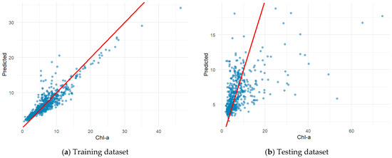
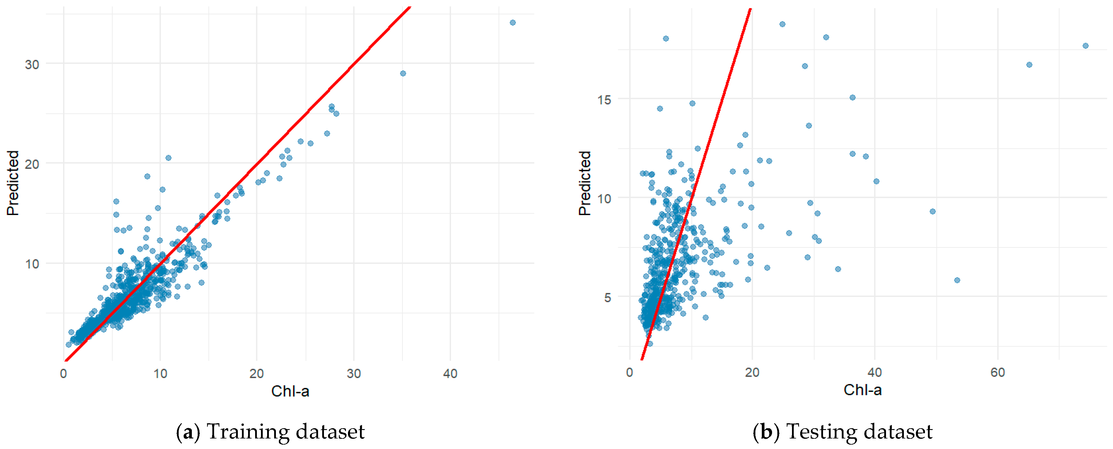
In the training dataset, the model achieved an RMSE of 2.13 and an MAE of 1.45, indicating relatively low prediction errors. The coefficient of determination (R²) reached 0.74, showing that the model explained a substantial proportion of the variability in the data used for model fitting. In the testing dataset, the RMSE and MAE increased to 4.58 and 3.26, respectively, while the coefficient of determination decreased to 0.42.

To further assess the predictive performance of the LightGBM model, Figure 3 compares observed and predicted chlorophyll-a concentrations for the training and testing datasets. In the training dataset (Figure 3a), most observations clustered around the identity line, indicating good agreement between observed and predicted chlorophyll-a concentrations. In the testing dataset (Figure 3b), however, observations were more widely scattered around the identity line, indicating a reduction in predictive performance. Furthermore, the model tended to underestimate higher chlorophyll-a concentrations, whereas predictions for low and moderate concentrations remained in closer agreement with the observed values.

Although the model did not achieve a perfect fit, the obtained R² value is consistent with those reported in previous studies on chlorophyll-a prediction models [56,57], reflecting the high variability of chlorophyll-a concentrations and the complexity of the processes governing their dynamics in aquatic ecosystems [58].

3.4. Feature Importance

The LightGBM model was trained using observations collected between 2017 and 2021 and evaluated on an independent validation dataset comprising observations from 2022 to 2023, as described in Section 2.2. The training subset was used to fit the LightGBM model, whereas the testing subset was used to evaluate its generalization ability and predictive performance on unseen data.

To optimize model performance, the main hyperparameters of the LightGBM algorithm were tuned. The final hyperparameter configuration consisted of a maximum of 80 leaves per tree, a maximum tree depth of 9, a minimum of 10 observations per leaf, a learning rate of 0.05, a feature fraction of 0.9 and a lambda L2 of 0.05.

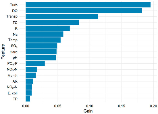
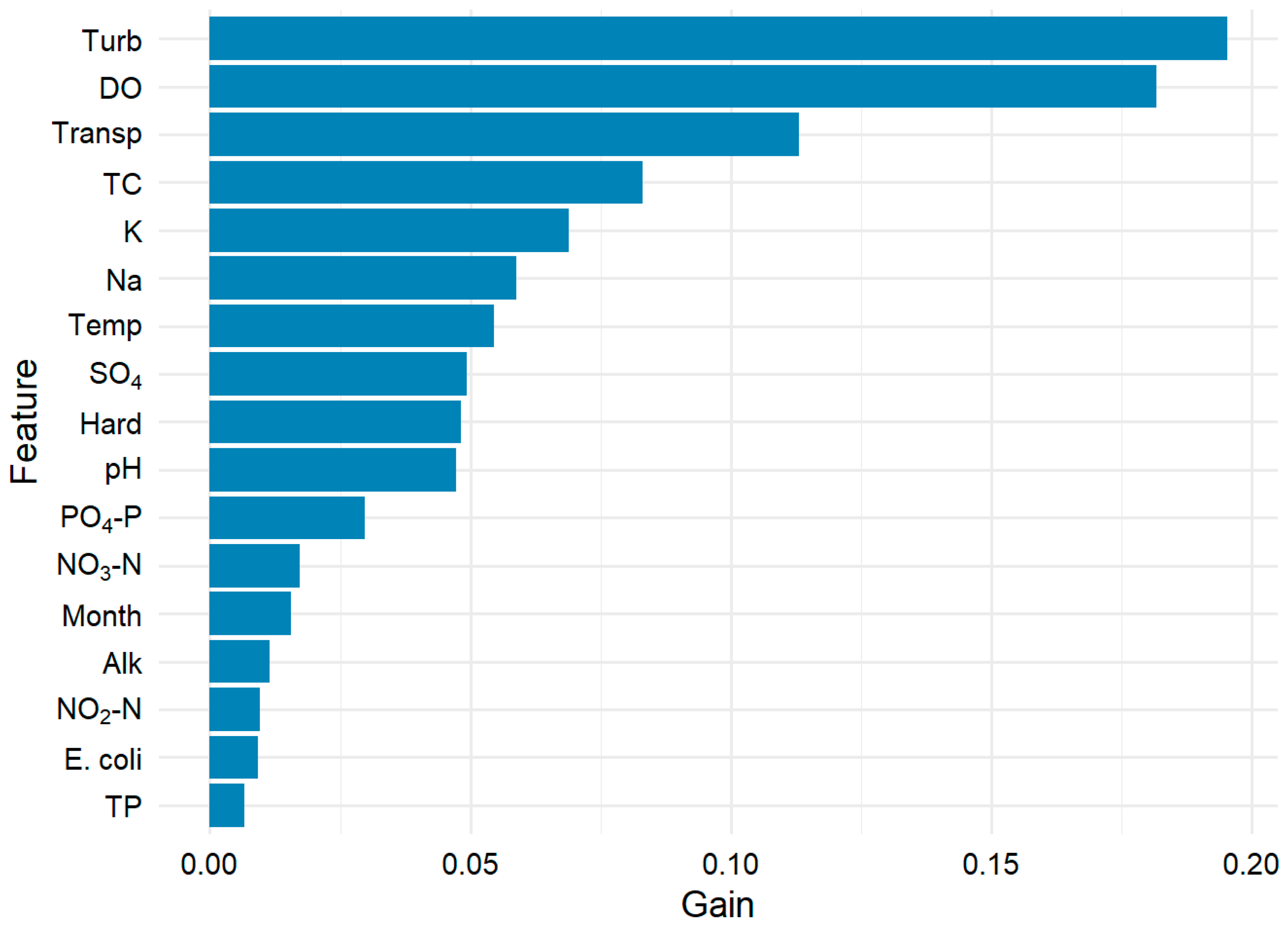
The relative importance of the physicochemical and biological predictor variables estimated by LightGBM is presented in Figure 4. This ranking identifies the variables contributing most to the prediction of chlorophyll-a concentrations and establishes a hierarchy of the most influential factors within the system.

The results showed that a small group of variables accounted for most of the predictive importance within the model. Turbidity (Turb) and dissolved oxygen (DO) emerged as the most influential predictors, reaching the highest gain values (approximately 0.20 and 0.18, respectively). These were followed by transparency (Transp), total coliforms (TC), potassium (K), and sodium (Na), which completed the group of variables with the greatest contribution to the predictive performance of the algorithm.

In contrast, total phosphorus (TP), E. coli, nitrite (NO₂-N), and alkalinity (Alk) exhibited gain values close to zero, suggesting a limited contribution to the model predictions. Although some of these variables displayed high extreme values in the previous descriptive analyses, they provided little additional predictive information compared with variables associated with the physical characteristics of the water and dissolved oxygen.

3.5. SHAP Analysis

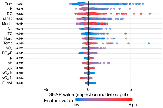
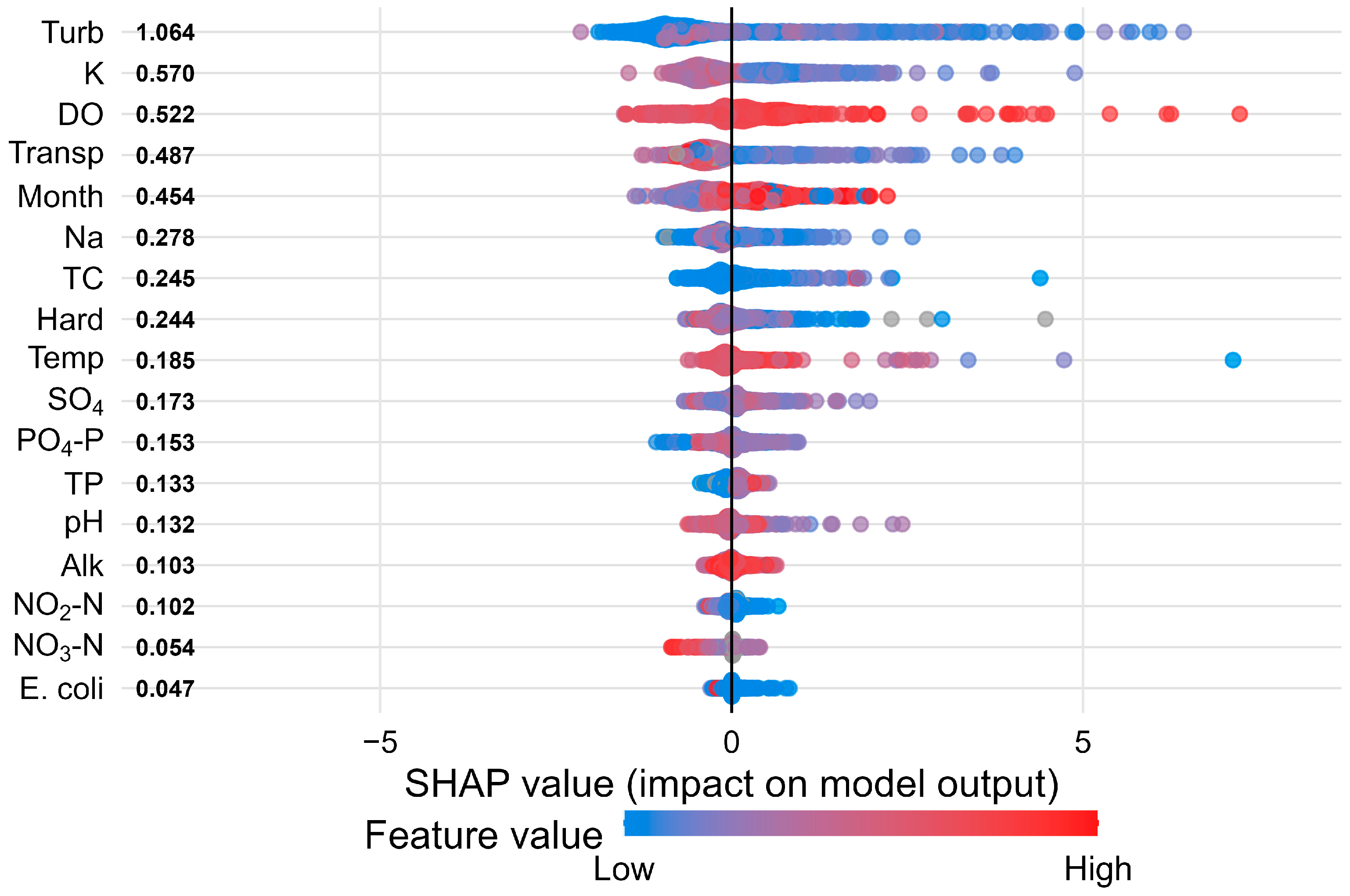
To interpret the behavior of the LightGBM model and quantify the contribution of each predictor variable to chlorophyll-a predictions, a SHAP analysis was performed. Figure 5 presents the SHAP summary plot, which ranks the predictor variables according to their relative importance, measured by their mean absolute SHAP values.

The plot provides information on both the magnitude and direction of the effect of each variable on the model predictions. Each point represents an individual observation; color indicates the value of the corresponding variable (red for high values and blue for low values), whereas its position along the horizontal axis reflects the contribution of that variable to the predicted chlorophyll-a concentration.

The SHAP summary plot (Figure 5) showed that turbidity (Turb) was the most influential predictor of chlorophyll-a concentrations, followed by potassium (K), dissolved oxygen (DO), transparency (Transp), and sampling month. These variables exhibited the highest mean absolute SHAP values (Turb = 1.064, K = 0.570, DO = 0.522, Transp = 0.487, and Month = 0.454), confirming their dominant contribution to the predictive performance of the model.

The direction of each variable’s effect can be inferred from the distribution of the points along the SHAP value axis. Turbidity (Turb) exhibited a clear inverse relationship with the model predictions: high values (red points) were predominantly associated with negative SHAP values, whereas low values (blue points) tended to cluster on the positive side of the SHAP axis, indicating that lower turbidity levels increased the predicted chlorophyll-a concentrations. A similar, albeit less pronounced, pattern was observed for transparency (Transp), where lower values were associated with positive contributions to the model predictions.

Dissolved oxygen (DO) ranked third in importance, with a mean absolute SHAP value of 0.522. In contrast to turbidity and transparency, higher dissolved oxygen concentrations (red points) tended to be associated with positive SHAP values, suggesting that increased dissolved oxygen levels contributed positively to the predicted chlorophyll-a concentrations.

Potassium (K) also made an important contribution to the model. However, the distribution of its SHAP values exhibited a more dispersed pattern without a clearly defined monotonic trend, suggesting the presence of nonlinear effects and potential interactions with other environmental variables.

The SHAP summary plot also identified sampling month as an influential predictor. This finding suggests that temporal variability associated with the seasonal cycle contributes to explaining changes in chlorophyll-a concentrations beyond the physicochemical and biological variables measured in this study.

In addition, sodium (Na), total coliforms (TC), hardness (Hard), temperature (Temp), sulfate (SO₄), phosphorus as phosphate (PO₄_P), total phosphorus (TP), and pH exhibited moderate-to-low contributions, with mean absolute SHAP values below 0.30, indicating a secondary role in the model predictions.

The nitrogen-related variables, including nitrite (NO₂-N) and nitrate (NO₃-N), together with E. coli, exhibited the lowest mean absolute SHAP values, indicating a relatively limited contribution to the predictive performance of the model under the conditions evaluated in this study.

Although the Gain-based importance and SHAP values showed slight differences in the ranking of the predictor variables, both approaches consistently identified the most relevant predictors of chlorophyll-a concentrations. The observed discrepancies in the secondary ranking are expected because the two metrics quantify variable importance from different perspectives: whereas Gain measures the improvement in the model’s objective function during training, SHAP quantifies the marginal contribution of each predictor to individual model predictions.

3.6. Generalized Linear Model Analysis

To complement the results obtained from the LightGBM and SHAP analyses, a GLM with a Gamma distribution and a logarithmic link function was fitted using the variables identified as the most relevant predictors. The objective was to evaluate the association between each predictor and chlorophyll-a concentrations and to determine which variables were statistically significant (

Table 5. Summary of the Generalized Linear Model.

Parameter	Estimate	95% CI	t Value	p-Value	VIF
Intercept	6.94	6.08 ± 7.92	28.69	<0.001
TC	1.04	1.00 ± 1.08	2.06	0.04	1.06
Hard	0.95	0.91 ± 0.99	−2.23	0.03	1.58
K	0.93	0.88 ± 0.98	−2.61	0.01	2.30
DO	1.06	1.01 ± 1.10	2.54	0.01	1.51
PO4-P	1.04	1.00 ± 1.09	2.11	0.04	1.34
Temp	0.92	0.88 ± 0.97	−3.34	<0.01	1.93
Transp	0.78	0.74 ± 0.82	−9.17	<0.001	2.39
Turb	0.85	0.81 ± 0.89	−6.55	<0.001	1.92

).

The GLM results (Table 5) showed that all predictors included in the model were statistically significant (p < 0.05). Total coliforms (TC), dissolved oxygen (DO), and orthophosphate (PO₄-P) were positively associated with the response variable, whereas hardness (Hard), potassium (K), temperature (Temp), transparency (Transp), and turbidity (Turb) showed negative associations.

Transparency exhibited the strongest association with the response variable, followed by turbidity and temperature, as indicated by the largest absolute t values. In addition, the variance inflation factor (VIF) values ranged from 1.06 to 2.39, well below the commonly accepted threshold of 5, indicating no evidence of relevant multicollinearity among the predictor variables and supporting the stability and reliability of the estimated coefficients.

Overall, the GLM results were consistent with those obtained from the LightGBM model, as both approaches identified the optical conditions of the water, particularly turbidity and transparency, as the most influential factors explaining the variability in chlorophyll-a concentrations in Lake Gatun.

4. Discussion

The LightGBM model achieved satisfactory predictive performance, highlighting the importance of accounting for nonlinear relationships and interactions among variables when modelling chlorophyll-a concentrations. Nevertheless, the model achieved lower predictive performance on the testing dataset than on the training dataset, suggesting that a substantial proportion of the variability in Chl-a concentration cannot be explained solely by the water quality variables included in this study.

The results obtained from the LightGBM model, SHAP and the GLM consistently identified turbidity and water transparency as the most relevant predictors explaining the variability of chlorophyll-a concentrations in Lake Gatun. Taken together, these findings suggest that phytoplankton dynamics in this tropical ecosystem are governed by the interaction of multiple physical, chemical, biological, and temporal factors, whose relationships are inherently complex and nonlinear. This interpretation is consistent with previous studies reporting that chlorophyll-a variability in aquatic ecosystems is driven by multifactorial mechanisms [59].

Turbidity emerged as the most influential predictor in both the variable importance analysis and the SHAP analysis, consistent with previous findings reported by Carneiro et al. [60]. This result agrees with the fundamental role of light availability in regulating phytoplankton productivity. Previous studies have shown that increased turbidity reduces the penetration of photosynthetically active radiation through the water column, thereby potentially limiting phytoplankton growth [61,62]. However, the observed relationship likely reflects more complex processes than light limitation alone.

In lake ecosystems, phytoplankton biomass itself contributes substantially to turbidity through the presence of suspended biogenic particles; consequently, both variables often exhibit covarying patterns closely associated with the trophic status of the system [63]. Therefore, the high predictive importance of turbidity may reflect not only hydrological processes related to the transport of suspended solids but also changes in phytoplankton biomass.

Dissolved oxygen was also strongly associated with chlorophyll-a concentrations, consistent with previous studies linking phytoplankton photosynthetic activity to dissolved oxygen levels in surface waters [62,64]. Although this association does not imply causality, it reflects the close interdependence between biological productivity and the metabolic processes that regulate water quality.

Furthermore, a negative association was identified between water transparency and chlorophyll-a concentrations. This finding agrees with previous studies reporting that elevated chlorophyll-a concentrations are associated with reduced light penetration through the water column [65]. Similarly, increased phytoplankton biomass and particulate matter have been shown to reduce water transparency through the absorption and scattering of solar radiation [66]. Because transparency integrates information related to suspended particles, organic matter, and phytoplankton biomass, its high predictive importance suggests that it is a relevant indicator of chlorophyll-a variability in Lake Gatun.

Another noteworthy finding was the high predictive importance of potassium. Although this element has received less attention than nitrogen and phosphorus in eutrophication studies, recent research suggests that potassium may act as an essential nutrient for cellular metabolism and phytoplankton growth, particularly in ecosystems where multiple factors simultaneously limit primary productivity [67].

In contrast, variables traditionally associated with eutrophication, including total phosphorus, orthophosphate, and inorganic nitrogen species, showed relatively low predictive importance. These findings differ from previous studies that identified total phosphorus as a variable significantly associated with chlorophyll-a concentrations [2], as well as from studies reporting nitrogen availability as the main factor associated with variations in this pigment [68].

In tropical ecosystems where nutrient availability remains relatively high throughout much of the year, chlorophyll-a variability may be driven more strongly by hydrological and climatic factors than by fluctuations in nutrient concentrations [69,70]. Under these conditions, nutrients may no longer act as the primary limiting factors, whereas other environmental processes become more influential in controlling phytoplankton biomass. This finding has direct implications for the design of water quality monitoring and management strategies in Lake Gatun.

In addition to the physicochemical and biological variables, the importance of the sampling month as a temporal predictor deserves particular attention. This finding highlights the relevance of seasonal processes in explaining the variability of Chl-a concentration in Lake Gatun. Panama has two well-defined climatic seasons that influence precipitation, runoff, water residence time, nutrient inputs, turbidity, and light availability. Together, these seasonal changes can indirectly affect phytoplankton dynamics, which likely explains why the inclusion of temporal information improved the predictive performance of the model, even after accounting for multiple physicochemical and biological variables.

Finally, integrating machine learning algorithms with traditional statistical approaches made it possible not only to identify the variables with the greatest predictive relevance but also to provide an ecologically meaningful interpretation of the observed associations. Explainable artificial intelligence techniques such as SHAP have proven effective for understanding the internal logic of tree-based models and identifying the variables that most strongly influence predictions in complex ecosystems [47,71,72,73]. In this context, the present findings contribute to a better understanding of the processes regulating chlorophyll-a dynamics in Lake Gatun and provide valuable information for the design of monitoring and water quality management strategies in one of Panama’s most important freshwater ecosystems.

One limitation of the present study is that observations from all monitoring stations were analyzed within a single predictive framework without explicitly modelling station-specific random effects or within-station temporal dependence. Although this approach is appropriate for identifying the environmental variables most strongly associated with chlorophyll-a concentrations at the scale of the entire lake, future work should consider hierarchical statistical models or spatiotemporal machine learning approaches to explicitly account for repeated measurements and spatial heterogeneity among monitoring stations.

In addition, future research could incorporate hydrometeorological variables, such as precipitation, streamflow, lake water level, solar radiation, and water residence time, as well as spatial information derived from remote sensing and higher-resolution temporal analyses. Incorporating these variables could improve the predictive performance of future models, assess the stability of the identified patterns under climate change scenarios, and provide a more comprehensive understanding of the mechanisms regulating Chl-a variability and phytoplankton dynamics in Lake Gatun.

5. Conclusions

The results obtained from the LightGBM model, SHAP and the GLM were highly consistent in identifying the main factors associated with chlorophyll-a concentrations, supporting the robustness of the observed patterns. Both LightGBM and the GLM identified turbidity as the predictor with the strongest association with chlorophyll-a concentrations. The LightGBM model demonstrated satisfactory predictive performance for estimating chlorophyll-a concentrations in Lake Gatun, achieving an RMSE of 4.58 and an MAE of 3.26. The SHAP analysis provided a transparent interpretation of the individual contribution of the predictor variables, facilitating the understanding of the relationships between environmental conditions and chlorophyll-a dynamics.

References

- Qin, J.; Ma, Z.; Li, Y. Review and Outlook for Research and Development in Aquatic Life and Ecosystems. Scilight 2025, 1, 2. [Google Scholar] [CrossRef] [Scilit]
- Huang, H.; Wang, W.; Lv, J.; Liu, Q.; Liu, X.; Xie, S.; Wang, F.; Feng, J. Relationship between Chlorophyll a and Environmental Factors in Lakes Based on the Random Forest Algorithm. Water 2022, 14, 3128. [Google Scholar] [CrossRef] [Scilit]
- He, Y.; Wang, X.; Xu, F. How Reliable Is Chlorophyll-a as Algae Proxy in Lake Environments? New Insights from the Perspective of n-Alkanes. Sci. Total Environ. 2022, 836, 155700. [Google Scholar] [CrossRef] [Scilit] [PubMed]
- Yomal, T.; Jayasinghe, A.; Deepananda, A.; Amarasinghe, U.; Jones, C. Trophic State of Dry Zone Reservoirs Utilized for Culture-Based Fisheries Development in Sri Lanka. J. Aquat. Sci. 2025, 30, 101–111. [Google Scholar] [CrossRef] [Scilit]
- Kim, Y.; Cho, I.; Kim, H.; Hwang, E.; Han, B. Assessing the Impact of Weirs on Water Quality and Phytoplankton Dynamics in the South Han River: A Two-Year Study. Water 2024, 16, 833. [Google Scholar] [CrossRef] [Scilit]
- Yuan, C.; Xu, Z.; Zhang, X.; Wei, Q.; Wang, H.; Wang, Z.; Chao, Y.; Zongjun, X.; Xuelei, Z.; Qinsheng, W.; et al. Photosynthetic Physiologies of Phytoplankton in the Eastern Equatorial Indian Ocean during the Spring Inter-Monsoon. Acta Oceanol. Sin. 2019, 38, 83–91. [Google Scholar] [CrossRef] [Scilit]
- Xu, W.; Duan, L.; Wen, X.; Li, H.; Li, D.; Zhang, Y.; Zhang, H.; Xu, W.; Duan, L.; Wen, X.; et al. Effects of Seasonal Variation on Water Quality Parameters and Eutrophication in Lake Yangzong. Water 2022, 14, 2732. [Google Scholar] [CrossRef] [Scilit]
- García–Nieto, P.J.; García–Gonzalo, E.; Alonso Fernández, J.R.; Díaz Muñiz, C. Forecast of Chlorophyll-a Concentration as an Indicator of Phytoplankton Biomass in El Val Reservoir by Utilizing Various Machine Learning Techniques: A Case Study in Ebro River Basin, Spain. J. Hydrol. 2024, 639, 131639. [Google Scholar] [CrossRef] [Scilit]
- Chen, R.; Ju, M.; Chu, C.; Jing, W.; Wang, Y. Identification and Quantification of Physicochemical Parameters Influencing Chlorophyll-a Concentrations through Combined Principal Component Analysis and Factor Analysis: A Case Study of the Yuqiao Reservoir in China. Sustainability 2018, 10, 936. [Google Scholar] [CrossRef] [Scilit]
- Jimeno-Sáez, P.; Senent-Aparicio, J.; Cecilia, J.M.; Pérez-Sánchez, J. Using Machine-Learning Algorithms for Eutrophication Modeling: Case Study of Mar Menor Lagoon (Spain). Int. J. Environ. Res. Public Health 2020, 17, 1189. [Google Scholar] [CrossRef] [Scilit] [PubMed]
- Paerl, H.W.; Otten, T.G. Harmful Cyanobacterial Blooms: Causes, Consequences, and Controls. Microb. Ecol. 2013, 65, 995–1010. [Google Scholar] [CrossRef] [Scilit]
- Ho, J.C.; Michalak, A.M.; Pahlevan, N. Widespread Global Increase in Intense Lake Phytoplankton Blooms since the 1980s. Nature 2019, 574, 667–670. [Google Scholar] [CrossRef] [Scilit]
- Deng, J.; Chen, F.; Hu, W.; Lu, X.; Xu, B.; Hamilton, D.P. Variations in the Distribution of Chl-a and Simulation Using a Multiple Regression Model. Int. J. Environ. Res. Public Health 2019, 16, 4553. [Google Scholar] [CrossRef] [Scilit] [PubMed]
- Shuvo, A.K.; Lottig, N.R.; Webster, K.E.; Delany, A.; Reinl, K.; Gries, C.; Smith, N.J.; Poisson, A.C.; McCullough, I.M.; Collins, S.M.; et al. LAGOS-US LIMNO: Data Module of Surface Water Chemistry from 1975–2021 for Lakes in the Conterminous U.S. Ver 5. Environmental Data Initiative. 2023. Available online: https://doi.org/10.6073/pasta/2c58f5a50ab813919f99cc1f265f271c (accessed on 11 March 2026).
- Díaz-Torres, O.; de Anda, J.; Lugo-Melchor, O.Y.; Pacheco, A.; Orozco-Nunnelly, D.A.; Shear, H.; Senés-Guerrero, C.; Gradilla-Hernández, M.S. Rapid Changes in the Phytoplankton Community of a Subtropical, Shallow, Hypereutrophic Lake During the Rainy Season. Front. Microbiol. 2021, 12, 617151. [Google Scholar] [CrossRef] [Scilit] [PubMed]
- Guimarães, B.M.D.M.; Neto, I.E.L. Chlorophyll-a Prediction in Tropical Reservoirs as a Function of Hydroclimatic Variability and Water Quality. Environ. Sci. Pollut. Res. 2023, 30, 91028–91045. [Google Scholar] [CrossRef] [Scilit] [PubMed]
- Malashenkov, D.; Zelalem, W. Phytoplankton Functional Groups and Size Diversity Reflect the Environmental Conditions and Trophic State in the High-Altitude Tropical Lake (Lake Tana, Ethiopia). SSRN Electron. J. 2022. [Google Scholar] [CrossRef] [Scilit]
- Woolway, R.; Kraemer, B.; Lenters, J. Global Lake Responses to Climate Change. Nat. Rev. Earth Environ. 2020, 1, 388–403. [Google Scholar] [CrossRef] [Scilit]
- Paerl, H.; Paul, V. Climate Change: Links to Global Expansion of Harmful Cyanobacteria. Water Res. 2012, 46, 1349–1363. [Google Scholar] [CrossRef] [Scilit] [PubMed]
- Jeppesen, E.; Meerhoff, M.; Davidson, T. Climate Change Impacts on Lakes: An Integrated Ecological Perspective Based on a Multi-Faceted Approach, with Special Focus on Shallow Lakes. J. Limnol. 2014, 73, 88–111. [Google Scholar] [CrossRef] [Scilit]
- Cubilla-Montilla, M.; Ramírez, A.; Escudero, W.; Cruz, C. Analyzing and Forecasting Vessel Traffic Through the Panama Canal: A Comparative Study. Appl. Sci. 2025, 15, 8389. [Google Scholar] [CrossRef] [Scilit]
- Canal de Panamá (ACP). Informe Anual de La Cuenca Hidrográfica Del Canal de Panamá: Sostenibilidad y Gestión Del Recurso Hídrico; ACP: Ciudad de Panamá, Panama, 2023.
- Cubilla-Montilla, M.; Carrasco, G.; Castillo, M. Assessment of Water Quality in the Panama Canal Watershed Using Multivariate Analysis of Physicochemical and Biological Parameters. Water 2025, 17, 979. [Google Scholar] [CrossRef] [Scilit]
- Hartshorn, N.; Marimon, Z.; Xuan, Z.; Cormier, J.; Chang, N.B.; Wanielista, M. Complex Interactions among Nutrients, Chlorophyll-a, and Microcystins in Three Stormwater Wet Detention Basins with Floating Treatment Wetlands. Chemosphere 2016, 144, 408–419. [Google Scholar] [CrossRef] [Scilit] [PubMed]
- Filstrup, C.T.; Downing, J.A. Relationship of Chlorophyll to Phosphorus and Nitrogen in Nutrient-Rich Lakes. Inland Waters 2017, 7, 385–400. [Google Scholar] [CrossRef] [Scilit]
- Phillips, G.; Pietiläinen, O.P.; Carvalho, L.; Solimini, A.; Lyche Solheim, A.; Cardoso, A.C. Chlorophyll–Nutrient Relationships of Different Lake Types Using a Large European Dataset. Aquat. Ecol. 2008, 42, 213–226. [Google Scholar] [CrossRef] [Scilit]
- Liu, Y.; Guo, H.; Yang, P. Exploring the Influence of Lake Water Chemistry on Chlorophyll a: A Multivariate Statistical Model Analysis. Ecol. Modell. 2010, 221, 681–688. [Google Scholar] [CrossRef] [Scilit]
- Çamdevýren, H.; Demýr, N.; Kanik, A.; Keskýn, S. Use of Principal Component Scores in Multiple Linear Regression Models for Prediction of Chlorophyll-a in Reservoirs. Ecol. Modell. 2005, 181, 581–589. [Google Scholar] [CrossRef] [Scilit]
- Paulino Borges, P.; Barreto Teresa, F.; Thomaz de Aquino Martins, P.; Carlos Nabout, J. Relative Influence of Direct and Indirect Environmental Effects on Sestonic Chlorophyll-a Concentration in Cerrado Streams Influência Relativa de Efeitos Ambientais Diretos e Indiretos Na Concentração Da Clorofila-a Planctônica Em Riachos Do Cerrado. Acta Limnol. Bras. 2015, 27, 301–310. [Google Scholar] [CrossRef] [Scilit]
- Qiu, X.C.; Zhao, H.X.; Sun, X.X. Studies on Relationship of Phytoplankton and Water Environmental Factors in Shahu Lake. Huan Jing Ke Xue 2012, 33, 2265–2271. [Google Scholar] [PubMed]
- Hadid, N.B.; Goyet, C.; Chaar, H.; Maiz, N.B.; Guglielmi, V.; Shili, A. Machine Learning Modeling Techniques for Forecasting the Trophic State in a Restored South Mediterranean Lagoon Using Chlorophyll-a in Connection with the Physico. Wetlands 2021, 41, 111. [Google Scholar] [CrossRef] [Scilit]
- Liao, Z.; Zang, N.; Wang, X.; Li, C.; Liu, Q. Machine Learning-Based Prediction of Chlorophyll-a Variations in Receiving Reservoir of World’s Largest Water Transfer Project—A Case Study in the Miyun Reservoir, North China. Water 2021, 13, 2406. [Google Scholar] [CrossRef] [Scilit]
- Yu, B.; Xu, L.; Peng, J.; Hu, Z.; Wong, A. Global Chlorophyll-a Concentration Estimation from Moderate Resolution Imaging Spectroradiometer Using Convolutional Neural Networks. J. Appl. Remote Sens. 2020, 14, 034520. [Google Scholar] [CrossRef] [Scilit]
- Zhu, W.; Liu, S.; Luan, K.; Xu, Y.; Liu, Z.; Cao, T.; Wang, P.; Verde, S.; Mastro, P.; Zhu, W.; et al. Research on the Inversion of Chlorophyll-a Concentration in the Hong Kong Coastal Area Based on Convolutional Neural Networks. J. Mar. Sci. Eng. 2024, 12, 1119. [Google Scholar] [CrossRef] [Scilit]
- Talamantes Murillo, J.M.; Luna Taylor, J.E.; Sánchez Pérez, E.D.; Castro Liera, M.A.; Santillán Méndez, I.M. Modelo de Regresión Basado En Redes Neuronales Artificiales Para La Estimación de La Concentración de Clorofila-a En El Pacífico Tropical Oriental Frente a Perú. Pädi Boletín Científico Cienc. Básicas Ing. ICBI 2026, 13, 111–118. [Google Scholar] [CrossRef] [Scilit]
- Busari, I.; Sahoo, D.; Sudheer, K.P.; Harmel, R.D.; Privette, C.; Schlautman, M.; Sawyer, C. Investigating the Influence of Measurement Uncertainty on Chlorophyll-a Predictions as an Indicator of Harmful Algal Blooms in Machine Learning Models. Ecol. Inform. 2024, 82, 102735. [Google Scholar] [CrossRef] [Scilit]
- Su, H.; Lu, X.; Chen, Z.; Zhang, H.; Lu, W.; Wu, W. Estimating Coastal Chlorophyll-A Concentration from Time-Series OLCI Data Based on Machine Learning. Remote Sens. 2021, 13, 576. [Google Scholar] [CrossRef] [Scilit]
- Song, Y.; Shen, C.; Hong, Y. Comparing the Performance of 10 Machine Learning Models in Predicting Chlorophyll a in Western Lake Erie. J. Environ. Manag. 2025, 380, 125007. [Google Scholar] [CrossRef] [Scilit] [PubMed]
- Mamun, M.; Kim, J.J.; Alam, M.A.; An, K.G. Prediction of Algal Chlorophyll-a and Water Clarity in Monsoon-Region Reservoir Using Machine Learning Approaches. Water 2020, 12, 30. [Google Scholar] [CrossRef] [Scilit]
- Samal, K.P.; Thakur, R.R.; Panda, A.K.; Nandi, D.; Pati, A.K.; Pegu, K.; Ðurin, B. Machine Learning-Enhanced Monitoring and Assessment of Urban Drinking Water Quality in North Bhubaneswar, Odisha, India. Limnol. Rev. 2025, 25, 44. [Google Scholar] [CrossRef] [Scilit]
- Al-Nuaami, W.A.H.; Dawod, L.A.J.; Kibria, B.M.G.; Ghorbani, S. Design and Implementation of a Deep Learning Model and Stochastic Model for the Forecasting of the Monthly Lake Water Level. Limnol. Rev. 2024, 24, 217–234. [Google Scholar] [CrossRef] [Scilit]
- Elhallaoui Oueldkaddour, F.Z.; Wariaghli, F.; Brirhet, H.; Yahyaoui, A.; Jaziri, H. Comparison of Machine Learning Models for Real-Time Flow Forecasting in the Semi-Arid Bouregreg Basin. Limnol. Rev. 2025, 25, 6. [Google Scholar] [CrossRef] [Scilit]
- Cuenca Hidrográfica—Autoridad Del Canal de Panamá. Available online: https://pancanal.com/cuenca-hidrografica/ (accessed on 11 March 2026).
- Fuentes, G.; Munim, Z.H. Climate Influence on Panama Canal Operations: Predicting Canal Water Times with Integrated Environmental and Operational Data. Transp. Res. E Logist. Transp. Rev. 2025, 203, 104319. [Google Scholar] [CrossRef] [Scilit]
- Rice, E.W.; Baird, R.B.; Eaton, A.D. Standard Methods for the Examination of Water and Wastewater, 23rd ed.; American Public Health Association: Washington, DC, USA, 2017. [Google Scholar]
- Ke, G.; Meng, Q.; Finley, T.; Wang, T.; Chen, W.; Ma, W.; Ye, Q.; Liu, T.-Y. LightGBM: A Highly Efficient Gradient Boosting Decision Tree. In Advances in Neural Information Processing Systems; Curran Associates: Red Hook, NY, USA, 2017; Volume 30. [Google Scholar]
- Lundberg, S.M.; Lee, S.-I. A Unified Approach to Interpreting Model Predictions. In Advances in Neural Information Processing Systems; Curran Associates: Red Hook, NY, USA, 2017; Volume 30, pp. 4766–4777. [Google Scholar]
- Li, L.; Qiao, J.; Yu, G.; Wang, L.; Li, H.Y.; Liao, C.; Zhu, Z. Interpretable Tree-Based Ensemble Model for Predicting Beach Water Quality. Water Res. 2022, 211, 118078. [Google Scholar] [CrossRef] [Scilit] [PubMed]
- Nelder, J.A.; Wedderburn, R.W.M. Generalized Linear Models. J. R. Stat. Soc. Ser. A Stat. Soc. 1972, 135, 370–384. [Google Scholar] [CrossRef] [Scilit]
- McCullagh, P. Generalized Linear Models; Routledge: Oxfordshire, UK, 2019; ISBN 9780203753736. [Google Scholar]
- Budakoti, S.; Pal, M. Prediction of Chlorophyll a Concentration and Analyzing Its Relationship with Environmental Factors in Lake Vänern Using Random Forest Algorithm. Limnology 2025, 27, 235–250. [Google Scholar] [CrossRef] [Scilit]
- Friedman, J.H. Greedy Function Approximation: A Gradient Boosting Machine. Ann. Stat. 2001, 29, 1189–1232. [Google Scholar] [CrossRef] [Scilit]
- Breiman, L.; Friedman, J.H.; Olshen, R.A.; Stone, C.J. Classification and Regression Trees; CRC Press: Boca Raton, FL, USA, 2017; ISBN 9781351460491. [Google Scholar]
- Hastie, T.J.; Pregibon, D. Generalized linear models. In Statistical Models in S; Routledge: Oxfordshire, UK, 2017; pp. 195–247. [Google Scholar]
- RStudio PBC. RStudio: Integrated Development for R, Version 4.2.1; RStudio PBC: Boston, MA, USA, 2022.
- Asres, B.W.; Kebedew, M.G.; Nerae, M.D.; Tsegaye, S.; Zimale, F.A. Remote Sensing-Based Estimation of Chlorophyll-a Concentrations in a Water Hyacinth-Infested Tropical Headwaters Lake: A Study of Lake Tana, Ethiopia. Front. Water 2025, 7, 1600222. [Google Scholar] [CrossRef] [Scilit]
- Malek, S.; Syed Ahmad, S.M.; Singh, S.K.K.; Milow, P.; Salleh, A. Assessment of Predictive Models for Chlorophyll-a Concentration of a Tropical Lake. BMC Bioinform. 2011, 12, S12. [Google Scholar] [CrossRef] [Scilit]
- Graeber, D.; McCarthy, M.J.; Shatwell, T.; Borchardt, D.; Jeppesen, E.; Søndergaard, M.; Lauridsen, T.L.; Davidson, T.A. Consistent Stoichiometric Long-Term Relationships between Nutrients and Chlorophyll-a across Shallow Lakes. Nat. Commun. 2024, 15, 809. [Google Scholar] [CrossRef] [Scilit]
- Contreras, F.; Castañeda, O.; Torres, R. Hidrología, Nutrientes y Productividad Primaria En Las Lagunas Costeras Del Estado de Oaxaca, México. Hidrobiológica 1997, 7, 9–17. [Google Scholar]
- Carneiro, F.M.; Nabout, J.C.; Vieira, L.C.G.; Roland, F.; Bini, L.M. Determinants of Chlorophyll-a Concentration in Tropical Reservoirs. Hydrobiologia 2014, 740, 89–99. [Google Scholar] [CrossRef] [Scilit]
- Kirk, J.T.O. Light and Photosynthesis in Aquatic Ecosystems; Cambridge University Press: Cambridge, UK, 1994; ISBN 9780521459662. [Google Scholar]
- Wetzel, R.G. Limnology Lake and River Ecosystems, 3rd ed.; Academic Press: San Diego, CA, USA, 2001; Volume 35, ISBN 9780127447605. [Google Scholar]
- Reynolds, C.S. The Ecology of Phytoplankton; Cambridge University Press: Cambridge, UK, 2006. [Google Scholar]
- Dodds, W.K.; Whiles, M.R. Freshwater Ecology: Concepts and Environmental Applications of Limnology; Academic Press: Cambridge, MA, USA, 2019. [Google Scholar]
- Zamora, L.F.C.; Bistrain, R.P.; Pérez-Vega, A.; Chávez, A.G.T.; Álvarez-Jara, M.; Martínez, R.I.V.; Mas, J.F. Estimación de La Concentración de Clorofila-a y Turbidez Con Imágenes Sentinel-2 En La Presa Cointzio, Michoacán, México. Investig. Geográficas 2026, 119, e61156. [Google Scholar] [CrossRef] [Scilit]
- Delegido, J.; Urrego, P.; Vicente, E.; Sòria-Perpinyà, X.; Soria, J.M.; Pereira-Sandoval, M.; Ruiz-Verdú, A.; Peña, R.; Moreno, J. Turbidity and Secchi Disc Depth with Sentinel-2 in Different Trophic Status Reservoirs at the Comunidad Valenciana. Rev. Teledetección 2019, 54, 15–24. [Google Scholar] [CrossRef] [Scilit]
- Sterner, R.W.; Elser, J.J. Ecological Stoichiometry; Princeton University press: Princeton, NJ, USA, 2003. [Google Scholar]
- Kuo, Y.M.; Chen, Y.H.; Chiu, Y.T.; Lin, T.F. Water Quality and Physicochemical Conditions Drive Chlorophyll-a Concentrations in Two Connected Subtropical off-Stream Reservoirs. Sustain. Environ. Res. 2025, 35, 15. [Google Scholar] [CrossRef] [Scilit]
- Jeppesen, E.; Nõges, P.; Davidson, T.A.; Haberman, J.; Nõges, T.; Blank, K.; Lauridsen, T.L.; Søndergaard, M.; Sayer, C.; Laugaste, R.; et al. Zooplankton as Indicators in Lakes: A Scientific-Based Plea for Including Zooplankton in the Ecological Quality Assessment of Lakes According to the European Water Framework Directive (WFD). Hydrobiologia 2011, 676, 279–297. [Google Scholar] [CrossRef] [Scilit]
- Gyllström, M.; Hansson, L.A.; Jeppesen, E.; García-Criado, F.; Gross, E.; Irvine, K.; Kairesalo, T.; Kornijow, R.; Miracle, M.R.; Nykänen, M.; et al. The Role of Climate in Shaping Zooplankton Communities of Shallow Lakes. Limnol. Oceanogr. 2005, 50, 2008–2021. [Google Scholar] [CrossRef] [Scilit]
- Joshi, N.; Ghoorkhanian, A.; Park, J.; Zhao, K.; Khanal, S. A Machine Learning-Based Assessment of Proxies and Drivers of Harmful Algal Blooms in the Western Lake Erie Basin Using Satellite Remote Sensing. Remote Sens. 2025, 17, 2164. [Google Scholar] [CrossRef] [Scilit]
- Kim, Y.W.; Kim, T.; Shin, J.; Lee, D.S.; Park, Y.S.; Kim, Y.; Cha, Y.K. Validity Evaluation of a Machine-Learning Model for Chlorophyll a Retrieval Using Sentinel-2 from Inland and Coastal Waters. Ecol. Indic. 2022, 137, 108737. [Google Scholar] [CrossRef] [Scilit]
- Jeong, B.; Chapeta, M.R.; Kim, M.; Kim, J.; Shin, J.; Cha, Y.K. Machine Learning-Based Prediction of Harmful Algal Blooms in Water Supply Reservoirs. Water Qual. Res. J. 2022, 57, 304–318. [Google Scholar] [CrossRef] [Scilit]
Disclaimer/Publisher’s Note: The statements, opinions and data contained in all publications are solely those of the individual author(s) and contributor(s) and not of MDPI and/or the editor(s). MDPI and/or the editor(s) disclaim responsibility for any injury to people or property resulting from any ideas, methods, instructions or products referred to in the content. |
© 2026 by the authors. Licensee MDPI, Basel, Switzerland. This article is an open access article distributed under the terms and conditions of the Creative Commons Attribution (CC BY) license.