


Abstract
Tropical lake ecosystems are vulnerable to degradation due to climate change and anthropogenic pressure. These dual pressures lead to ecological change and alterations in aquatic parameters, including chlorophyll-a (Chl-a). Lake Poso is the third-largest lake in Indonesia; Chl-a variability and phenology in this tropical lake remain understudied due to brief observational records. This study characterizes the spatiotemporal variability and phenology of Chl-a in Lake Poso, Indonesia, over two decades (2003–2025) to establish a multi-decadal baseline and detect early indications of increasing phytoplankton biomass. Chl-a was derived from combined Terra and Aqua MODIS observations processed in Google Earth Engine, followed by trend, phenological, and spatial analyses. Results reveal a significant increase in annual Chl-a and a general upward tendency across the study period. Climatological reconstruction identifies a distinct bimodal phenology, with a primary peak in December and a secondary peak in April. Interannual trends show no significant shift in Start of Season timing; however, primary peak magnitudes tend to increase (+0.079 mg m−3 yr−1), largely influenced by extreme episodic anomalies. Spatial analysis reveals heterogeneous increases in Chl-a, particularly in the central and northern zones. These findings suggest a possible early trajectory toward higher phytoplankton biomass and establish the first satellite-derived multi-decadal Chl-a baseline for Lake Poso.
1. Introduction
Global ecosystems, including freshwater systems, are being substantially reshaped by climate change [1]. Beyond climate pressure, freshwater ecosystems worldwide are simultaneously burdened by anthropogenic activities and catchment-scale environmental change, making them increasingly susceptible to ecological degradation [2,3,4]. In lakes, Chl-a is an important indicator of ecosystem conditions. It is used to quantify phytoplankton biomass, trophic status, and aquatic ecosystem health and degradation [5,6]. Analyzing strong Chl-a variability is crucial for understanding lake phytoplankton biomass patterns, phenological shifts, and the potential for ecosystem degradation, which may be associated with climate change and anthropogenic pressures [7]. Beyond changes in mean Chl-a concentration, the seasonal organization of phytoplankton biomass, commonly referred to as Chl-a phenology, provides additional ecological information on when productivity begins to increase, when seasonal peaks occur, how intense those peaks are, and how long elevated productivity persists within an annual cycle [8,9].
Current studies on long-term lake Chl-a variability are dominated by temperate [10,11,12] and subtropical regions, where Chl-a dynamics are driven by seasonal fluctuations in lake temperature and stratification, as well as light and nutrient availability [13,14,15]. In contrast, research on Chl-a variability and lake phenology in equatorial regions, including Indonesia, is relatively rare [16]. Indonesia has over 840 lakes and 162 dams, but there are limited systematic studies on long-term Chl-a characteristics and trends [17,18]. Previous studies in Indonesia have been conducted at Lake Towuti, Rawapening, and Lake Warna, using paleolimnological approaches, including sediment core analysis, to reconstruct past conditions [16,19,20,21]. However, there remains a profound lack of literature that explores Chl-a variability through continuous time-series monitoring and phenological analysis [22]. These lakes may be influenced not only by local catchment processes, but also by monsoonal rainfall and large-scale climate anomalies such as El Niño-Southern Oscillation (ENSO), which may affect hydrological inputs, water-column stability, and phytoplankton productivity.
Lake Poso is the third largest and one of the oldest tropical lakes in Central Sulawesi, Indonesia. As an ancient lake formed through tectonic activity, Lake Poso is characterized by high levels of endemic biodiversity and long sediment records accumulated over geological timescales. These characteristics make ancient lakes particularly sensitive indicators of long-term environmental change, as their biological communities have co-evolved with regional climate dynamics and are therefore more vulnerable to novel anthropogenic and climatic pressures compared to younger lake systems [23,24]. The lake plays an important role in the local community, serving as a means of transportation and supporting agriculture, fisheries, tourism, and surrounding settlements. Other pressures affecting changes in the ecological condition of Lake Poso include land-cover changes within the catchment area. Hydrological modification of the lake upstream to optimize water storage capacity has altered seasonal water fluctuations, leading to the accumulation of organic matter in the shallow zone. This condition causes changes in Total Suspended Solids, Dissolved Oxygen, Chemical Oxygen Demand, Nitrate, and phosphorus [25,26]. Deforestation in the catchment area due to plantation activities, agricultural expansion, and natural forest canopy loss has increased soil erosion, leading to sedimentation and nutrient transport to the water body [25,27].
A historical study by Lehmusluoto et al. [28] in the early 1990s shows that Lake Poso had an oligotrophic (low productivity) status. However, the recent studies by Sulawesty et al. [29] and Kaban et al. [27] found that Poso Lake has a mesotrophic to eutrophic status. These phenomena may be associated with increased nutrient intake and other factors, such as erosion and sedimentation, that lead to eutrophication, which has multidimensional consequences for water and ecological quality, as well as socioeconomic impacts [30,31,32,33]. However, the extent to which these reported trophic changes are expressed in long-term Chl-a variability, seasonal timing, and spatial distribution remains poorly understood. Water quality monitoring in Indonesia’s lakes, including Poso, is generally conducted in a fragmented and limited snapshot of time points, such as single-season surveys [27,29], solitary [25], and short-term temporal [34]. As a result, the historical record is too brief to capture actual temporal variations in Chl-a. This limitation complicates interpretation, as single measurements may reflect only short-lived anomalies or temporary seasonal shifts rather than long-term trends [8,35].
This fundamental limitation of continuous, spatially consistent data can be overcome through satellite remote sensing, which offers systematic, repeated observations across entire lake surfaces and provides the long-term historical archive necessary for robust phenological and trend analysis. In recent years, several studies have applied satellite remote sensing to monitor Chl-a and other water-quality parameters in Indonesian and Southeast Asian inland waters [36]. Used Landsat 8 OLI imagery for multitemporal Chl-a monitoring in Lake Matano and Lake Towuti, demonstrating the applicability of medium-resolution satellite data for relatively clear Indonesian lakes but also highlighting the influence of atmospheric correction uncertainty on Chl-a estimation [37]. Assessed remote sensing of water quality in Lake Toba by constructing satellite-based time series of turbidity and Chl-a as indicators of eutrophication, while Lalovic et al. [37] used Sentinel-2 imagery to estimate several water-quality parameters, including Chl-a, in Lake Rawa Pening. At the Southeast Asian scale, satellite observations have also been used to estimate Chl-a and monitor algal blooms in Laguna de Bay, Philippines, using Sentinel-2 and Sentinel-3 data [38,39]. These studies provide an important foundation for remote sensing of inland waters in the region. However, they have generally focused on algorithm evaluation, Chl-a estimation, short-term spatial mapping, validation against field measurements, limited image-date comparisons, or event-based monitoring, rather than continuous multi-decadal reconstruction of Chl-a variability and phenology [36,37,40]. Although high-resolution imagery such as Sentinel-2, Landsat 8/9, or Planetscope is ideal for analysis in confined areas such as lakes, their revisit frequency and historical continuity may be less suitable for extracting consistent multi-decadal phenological metrics. Whereas sensors such as Moderate Resolution Imaging Spectroradiometer (MODIS) provide high-frequency observation and have been available since the early 2000s, offering an opportunity to reconstruct long-term Chl-a variability at monthly, seasonal, interannual, and phenological scales. Remote sensing data are crucial for analysis of long-term variability within a climatological framework.
Previous long-term time-series research on lake Chl-a was conducted by Cao et al. [41], who analyzed variability in eutrophic Lake Taihu (China) from 1984 to 2019. Similarly, Palmer et al. [8] demonstrated that satellite remote sensing can be used to retrieve and map phytoplankton phenology in Lake Balaton (Hungary) using ten years of Medium Resolution Imaging Spectrometer (MERIS) satellite time-series data, while Maeda et al. [35] reconstructed more than three decades of Landsat-derived Chl-a in high-latitude Finnish lakes to examine temporal shifts in phytoplankton phenology. Collectively, these studies demonstrate that satellite time-series data extend beyond spatial Chl-a mapping, enabling the quantification of bloom phenology, including timing of onset, peak magnitude, bloom duration, and interannual trajectories, across multi-decadal observation windows. Although satellite studies have been conducted in Indonesia and Southeast Asia, long-term analyses are still lacking to understand monthly, seasonal, and interannual changes, long-term trends, the timing and magnitude of blooms, and how these patterns vary in tropical lakes. To date, no study has reconstructed a continuous multi-decadal MODIS-derived Chl-a time series for Lake Poso that simultaneously addresses long-term trend detection, phenological characterization, and spatial heterogeneity, leaving a critical gap in understanding productivity dynamics of this ancient tropical lake over climate-relevant timescales.
Consequently, a systematic assessment of multi-decadal Chl-a dynamics in tropical lakes is imperative to elucidate how these ecosystems respond to the interplay of regional monsoonal forces and global climatic anomalies. The current study aimed to investigate the spatio-temporal variability, phenological patterns, and long-term trends of MODIS-derived Chl-a concentration in Lake Poso, Indonesia, spanning 2003 to 2025 using combined Terra and Aqua observations. Specifically, this study seeks to (1) characterize the monthly, seasonal, and interannual variability of Chl-a concentration over more than two decades; (2) identify long-term trends and phenological characteristics of Chl-a dynamics, including the timing, magnitude, and persistence of seasonal productivity peaks; and (3) examine the spatial heterogeneity of Chl-a concentration across Lake Poso to determine whether distinct lake zones exhibit different productivity patterns.
2. Materials and Methods
2.1. Study Area
Lake Poso is located in Poso Regency, Central Sulawesi Province, Indonesia (coordinates range from 1°44′40.7″ S to 2°03′41.2″ S and 120°30′46.3″ E to 120°42′49.1″ E; Figure 1). The lake is an ancient tectonic lake and is situated at approximately 485 m above sea level. Recent studies describe Lake Poso as the third-largest lake in Indonesia, with a surface area of approximately 368.9 km2 and a maximum depth of approximately 400 m [25]. This lake lies in the collision zone between the Eurasian and Pacific tectonic plates, over metamorphic bedrock. The local climate around Lake Poso is humid tropical, with an average annual rainfall of 3075 mm. The rainy season peaks in April and May, and the dry season in August and September. Rainfall in these areas is influenced by Sea Surface Temperature (SST) variability in the western Pacific and ENSO [42].
Figure 1.
Study area.
Indonesia has three main rainfall patterns: monsoon, equatorial, and local. The Lake Poso catchment lies within the equatorial rainfall zone, receiving two rainfall peaks annually linked to the northward and southward migration of the Inter-Tropical Convergence Zone (ITCZ) across the equator. The ITCZ’s six-month cycle provides a persistent signal marking the onset of the rainy season. This is reflected in the average monthly rainfall climatology from Climate Hazards Center Infrared Precipitation with Stations (CHIRPS) data (2003–2025) in the Lake Poso watershed, which shows two distinct rainfall peaks. The first and highest rainfall is in April, with a secondary peak in November, separated by a dry-season minimum in August (Figure 2).
Figure 2.
Climatological mean monthly rainfall over the Lake Poso watershed based on CHIRPS data for 2003–2025.
2.2. Data Acquisition
This study uses the MODIS sensor for Chl-a analysis, which was acquired and analyzed in Google Earth Engine (GEE), a cloud computing platform highly effective for temporal and spatial data analysis. To ensure data availability, we used both Terra MODIS (MOD09GA.061) and Aqua MODIS (MYD09GA.061) daily surface reflectance products over the observation period from January 2003 to December 2025.
The MOD09GA and MYD09GA Version 6.1 products provide atmospherically corrected surface reflectance for MODIS bands 1–7, with 500 m surface reflectance bands and 1 km observation and quality assurance layers. Because both Terra and Aqua observations were used, the combined dataset increased temporal sampling density and reduced data gaps caused by cloud contamination, scan geometry, and missing observations. Chl-a is calculated separately for each daily Terra and Aqua image. The daily Chl-a values from both sensors are then combined into a monthly composite using a per-pixel median, which is robust to outliers and residual cloud contamination. Combining both sensors also increases the number of valid daily observations available for each monthly composite, improving temporal representativeness relative to using a single sensor’s overpass alone. However, no explicit correction was applied for potential systematic differences between Terra and Aqua arising from their distinct overpass times or from long-term sensor calibration drift, as concurrent in situ data needed to characterize such differences were not available for Lake Poso.
The study area boundaries were precisely defined to ensure spatial consistency over two decades of observation. We applied the Normalized Difference Water Index (NDWI) on the Landsat 7 ETM (2003) and Landsat 8 OLI imagery to delineate the water surface area. The extraction results were overlaid to construct a temporally consistent water mask representing the stable open-water surface of Lake Poso during the study period. To ensure accurate Chl-a extraction, a 1500 m internal buffer zone from the lakeshore was applied. These procedures are crucial for removing spectral noise along the shoreline, reducing the adjacency effect of land reflectance, avoiding interference from water-bottom reflectance in the shallow littoral zone, and eliminating Chl-a detection from aquatic plants along the lake shore [43,44]. The final analysis mask therefore represents the inner open-water zone of Lake Poso and was used consistently for all temporal, phenological, trend, and spatial analyses.
2.3. Pre-Processing
The preprocessing procedure was applied in GEE to minimize bias caused by atmospheric disturbances. This step is necessary given the characteristics of the tropical region, with high cloud cover and humidity. To ensure the quality of surface reflectance data, we applied the atmospheric and Cloud Masking algorithm using bitwise operations on the MODIS quality bands by extracting information from the state_1 km and QC_500 m bands. In the state_1 km band, several bitwise operations are used to identify and remove pixels detected as cloud (bits 0–1), cloud shadows (bit 2), and the internal cloud algorithm flag (bit 10). The information in the QC_500 m band was processed to evaluate sensor integrity at 500 m resolution, ensuring that only the best reflectance estimates are used in analysis.
Although the study area boundaries were defined by overlaying NDWI extraction and buffer areas, red-band-based filtering was applied to ensure the quality of water pixels. This filtering process used the reflectance pixel value to identify and remove pixels with negative or zero reflectance values, producing only positive pixel values. Negative and zero reflectance indicate a very dark cloud shadow, sensor detection failure, or a shadow-edge pixel that passes the bitwise correction [45]. This additional filtering step was used as a conservative quality-control procedure to ensure that Chl-a estimation was applied only to valid water pixels.
2.4. Algorithm and Data Processing
The Chl-a concentration was estimated using a 4th-order polynomial empirical model based on the NASA Ocean Color 3 for MODIS (OC3M) Algorithm [46,47], as adapted to the spectral band configuration of the MOD09GA/MYD09GA surface reflectance product [48]. This algorithm uses the band-ratio reflectance values at the blue and green wavelengths to identify phytoplankton pigment absorption in water optics. The physical basis of this approach is that Chl-a strongly absorbs light at the blue wavelength while reflecting green wavelengths. Hence, an increasing Chl-a concentration yields a progressively smaller blue-to-green reflectance ratio [49]. The standard OC3M formulation requires remote sensing reflectance (Rrs) to be derived from the maximum of the two blue channels (443 nm, 488 nm) and the green channel (547 nm) [50]. However, the MOD09GA/MYD09GA product provides only seven land surface reflectance bands (B01–B07) and does not include the 443 nm or 488 nm bands. Consequently, a single-band adaptation, Band 3 (469 nm), was used as the blue proxy and Band 4 (555 nm) as the green reference, following precedents in the inland water remote sensing literature [51,52]. It is important to note that MOD09GA provides atmospherically corrected land surface reflectance (ρsur), which is conceptually distinct from above-surface remote sensing reflectance (Rrs) for which OC3M was originally formulated. The atmospheric correction applied in MOD09GA (MAIAC-based or standard 6S) is optimized for land surfaces and does not include the aerosol and sun-glint corrections specific to open-water retrievals. Furthermore, because MODIS Bands 3 and 4 were substituted for the standard OC3M bands and the original polynomial coefficients were applied directly without site-specific field calibration, the model lacks direct empirical validation. Consequently, the derived Chl-a values must be interpreted strictly as a relative proxy for phytoplankton biomass rather than absolute, validated concentrations. Absolute values should not be interpreted as direct equivalents of laboratory-measured chlorophyll-a concentrations because no local calibration or validation dataset was available. This approach is nonetheless consistent with recent inland water studies that have applied land-optimized surface reflectance products for long-term Chl-a trend analysis in the absence of water-specific atmospheric correction [51,52]. The main indicator of this algorithm is the spectral ratio between the surface reflectance at the Blue channel/Band 3 (459–479 nm) and the Green channel/Band 4 (545–565 nm), calculated using Equation (1).
The Chl-a value, expressed as a nominal concentration (mg m−3), was retrieved using a fourth-order polynomial function of X, as defined in Equation (2):
where the coefficients are , standard OC3M polynomial coefficients in NASA OCv6 (https://oceancolor.gsfc.nasa.gov/data/reprocessing/r2009/ocv6/, accessed on 20 December 2025). To ensure the reliability and validity of the Chl-a value, we remove outlier data that may be caused by sun glint or thin cloud cover. The Chl-a estimation values are limited to the range of 0 to 100 mg m−3.
2.5. Data Analysis
2.5.1. Chlorophyll-a Analysis
Chl-a estimation was conducted on daily MODIS data. We applied a composite aggregation process and used the median operator to produce monthly composite data, mitigating extreme and null values caused by atmospheric contamination or those that remained after cloud masking. We also applied annual and seasonal aggregation to produce the spatial composite of Chl-a concentration using the mean operator. Due to cloud-cover dynamics in Central Sulawesi, we also applied quality control to data based on percent cover. The cloud-masking process may leave only a small portion of the image available for Chl-a analysis, resulting in a generalized Chl-a profile. To ensure spatial representativeness of monthly composites while retaining sufficient temporal coverage given the high cloud frequency of the tropical study region, a month was retained for analysis only if at least 25% of pixels within the inner buffer zone were cloud-free. This threshold was selected to balance data completeness and the risk of spatial bias introduced when composites are derived from a very small fraction of available pixels. The months that do not meet this threshold are labeled “NaN” and excluded from the composite and statistical analyses.
The Chl-a concentration processing results are exported as a raster (.tif), and the pixel values are extracted into a monthly tabular format for further analysis over 23 years. Temporal analyses are conducted to cover monthly, seasonal, and interannual variability. Long-term trends were identified using the moving average method to eliminate short-term anomalies and reveal systematic patterns of Chl-a concentration changes throughout the study period/Spatial pattern analysis was conducted through visual and quantitative interpretation of Chl-a concentration distributions in annual and seasonal climatology composites to identify the spatial dynamics of Chl-a distribution in the study area.
2.5.2. Phenology Analysis
Phenology is a scientific discipline that studies the timing of periodic events in the life cycles of flora and fauna, which are significantly influenced by environmental conditions and climate pressure [53]. Over time, this terminology has also been widely applied to represent the biological event [54]. Measuring phenological metrics is essential for quantifying organisms’ life cycles and estimating shifts in biological responses due to environmental change [53]. Understanding these phenological patterns is important for assessing the ecological status of a water body and identifying factors driving environmental changes, such as temperature stratification, solar radiation, and ice cover. A study by Maeda et al. [35] examined the seasonal patterns and temporal dynamics of phytoplankton blooms.
To get a comprehensive understanding of Chl-a seasonal dynamics, we applied phenological analysis using a hydrologically based time-series reconstruction rather than the standard calendar (January–December) to produce a representative pattern of results. We used the hydrological year that runs from July to June. This setting aims to show the transition from the dry season (August–September) to the wet Season in one cycle, which is driven by the northward shift in the Inter-Tropical Convergence Zone (ITCZ) and modulated by ENSO variability [55,56]. The discrete monthly composite data were converted into a continuous daily time series (365 days) using a standard Cubic Spline interpolation (k = 3) technique. This method can produce smooth curves while preserving the pattern’s characteristics without introducing extreme artificial oscillations. These daily curves serve as the primary basis for extracting phenological metrics with higher temporal resolution.
The long-term monthly data (2003–2025) are grouped by hydrological months to create the climatology pattern. We analyzed several phenology metrics, including Start of Season (SOS), End of Season (EOS), Peak of Season (POS), and Position of Trough (POT). SOS is the midpoint of the early Chl-a bloom phase, indicating the first day on which the Chl-a concentration exceeds the threshold (>40%), marking the start of a consistent uptrend (minimum of 10 days). POS refers to the day of the year on which the reconstructed Chl-a curve reaches its maximum value within the defined hydrological year, representing the timing of maximum seasonal phytoplankton biomass or Chl-a concentration [8,35]. For example, if the maximum reconstructed Chl-a value occurs in October within the July–June hydrological cycle, the POS is assigned to the corresponding day in October. EOS indicates the time point after the POS at which it moves below the threshold. POT shows the lowest Chl-a value in a cycle. We used a threshold of 40% of the annual concentration, as defined in Equation (3).
The 40% amplitude threshold was used to identify the onset and decline of elevated Chl-a conditions while reducing sensitivity to short-lived fluctuations. Relative amplitude thresholds are commonly used in phenological studies to extract seasonal transition points from smoothed biological time series. However, the selected threshold should be interpreted as an operational definition of seasonal Chl-a increase rather than a universal ecological boundary.
Based on the literature, there is no absolute threshold for determining phenological metrics such as SOS and EOS; it largely depends on the signal-to-noise ratio and seasonal amplitude characteristics of the study site [57,58]. Previous studies have widely used thresholds ranging from 10% [58] to 15–35% [59,60,61] and up to 50%. Comprehensive evaluations by Ren et al. [62] suggest an optimal range of 25–40%. A stricter 50% threshold has also been used, particularly for high-latitude lakes with freeze-driven blooms [35]. Therefore, the 40% threshold is considered sufficient to capture the early and end phases of biological growth affected by monsoon variability.
In addition to the climatological analysis, trend analysis was used to evaluate shifts in the pattern of Chl-a concentration over time. The trend shift was analyzed using a deviation index, calculated each year relative to the long-term climatological means, with the Mann–Kendall and Sen’s Slope Estimator.
2.5.3. Spatial Variability Analysis
Spatial variability analysis was conducted to examine the heterogeneity of Chl-a concentration across Lake Poso. The study aims to determine whether distinct lake zones have different productivity patterns. Seasonal and annual climatological composites were generated from valid Chl-a pixels during 2003–2025. These composites mapped the long-term mean spatial distribution of Chl-a. They also identified persistent high- and low-concentration areas within the inner open-water zone. Subsequently, for seasonal variability, the seasonal mean data are based on the standard seasonal period (DJF, MAM, JJA, SON).
Pixel-based descriptive statistics, including monthly, seasonal, and annual mean, were calculated to quantify the magnitude and stability of spatial Chl-a patterns. Spatial interpretation explored differences between central open-water areas and zones near potential catchment or hydrological influences. The 1500 m internal buffer was applied to minimize shoreline adjacency effects. The resulting spatial products supplement temporal and phenological analyses. They help determine whether long-term Chl-a dynamics are spatially homogeneous or whether some Lake Poso zones consistently exhibit distinct productivity.
3. Results
3.1. Temporal Variability
3.1.1. Monthly Variability
Valid-pixel coverage across the retained monthly composites was at least 25%, with the majority of months (66%) exceeding 75% coverage and 85% exceeding 50% coverage. Only 16% of retained months fell within the 25–50% coverage range. Figure 3 illustrates the monthly trend of Chl-a variability in the study area. The results indicate a general increase in Chl-a concentration, with 10 of 12 months showing an upward trend. However, after applying temporal autocorrelation using the Trend-Free Pre-Whitening (TFPW) and multiple comparisons with the False Discovery Rate (FDR) method, no statistically significant increasing trends were detected. The strongest monthly increase occurred in December (Sen’s slope = 0.0769 mg m−3 yr−1 [95% CI: 0.0180, 0.1500], τ = 0.4526, p = 0.0698). Notably, April exhibited pronounced interannual variability, with high Chl-a values in 2016 and 2022, while in the previous decade, the values for that month consistently remained below 3 mg m−3. In July, recurrent spikes in Chl-a were recorded in several years: 2007 (4.44 mg m−3), 2013 (4.39 mg m−3), 2020 (3.23 mg m−3), and 2022 (6.93 mg m−3). In contrast, a downward trend was identified in February and August. March, May, and October displayed relatively stable interannual variability compared with highly volatile months such as April, July, and December. Overall, the monthly analysis reveals that long-term Chl-a intensification in Lake Poso is temporally asymmetric during the October–December transition period, but not statistically significant. This pattern may indicate that the processes associated with higher Chl-a concentrations are most active during the onset of the wet season but exhibit high interannual variability rather than a consistent long-term trend.
Figure 3.
Monthly trends of MODIS-derived Chl-a in Lake Poso, 2003–2025. The red dotted lines indicate the Sen’s slope trendline.
3.1.2. Seasonal Variability
Figure 4 illustrates the seasonal variability of Chl-a from 2003 to 2025, divided into four periods: December, January, and February (DJF); March, April, and May (MAM); June, July, and August (JJA); and September, October, and November (SON). The findings indicate that DJF has the highest ensemble mean of Chl-a, at 2.33 mg m3, along with the greatest variability. In contrast, SON has the lowest mean at 1.97 mg m−3 and exhibits the most stable trend. Across all seasons, there is an upward trend, but the Mann–Kendall results show that only SON exhibited a statistically significant increase (Sen’s slope = 0.0276 mg m−3 yr−1, τ = 0.4348, p = 0.0040). MAM also showed a positive tendency (Sen’s slope = 0.0259 mg m−3 yr−1, τ = 0.2925), although the trend was only marginally significant (p = 0.0538). DJF and JJA showed weaker and non-significant trends. These results suggest that the long-term Chl-a increase was most statistically robust during the SON season, primarily because its low interannual variability enhanced the signal-to-noise ratio. In contrast, the absolute maximum biomass and strongest interannual fluctuations remained concentrated during the DJF period.
Figure 4.
Seasonal means (averaged over three months) of MODIS-derived Chl-a in Lake Poso, 2003–2025: DJF (December–January–February), MAM (March-April-May), JJA (June–July August), and SON (September–October–November). The dot lines indicate the Sen’s slope trendline.
3.1.3. Annual Variability
At the interannual scale, annual mean Chl-a concentration (Figure 5) ranged from 1.52 to 3.47 mg m−3, with the lowest value recorded in 2005 and the highest in 2022. The mean Chl-a concentration over the full study period was 2.14 mg m−3 (SD = 0.42), a value broadly consistent with mesotrophic conditions based on proxy-derived Chl-a estimates. Annual Chl-a remained mostly below 2 mg m−3 during 2003–2008, increased episodically in 2009 and 2013, and became more variable after 2021. The highest annual mean in 2022 exceeded the previous major peak in 2009, while Chl-a in 2025 remained among the highest values in the 23-year record. The Mann–Kendall test indicated a statistically significant increasing trend in annual Chl-a concentration (τ = 0.3162, p = 0.0369), with a Sen’s slope of 0.0270 mg m−3 yr−1. This indicates a gradual long-term increase in annual Chl-a, accompanied by a recent period of enhanced variability and elevated annual concentrations during 2022–2025.
Figure 5.
Annual variability and Mann–Kendall trend of MODIS-derived Chl-a in Lake Poso, 2003–2025. Error bars represent the standard error of the mean (SEM). The red dotted lines indicate the Sen’s slope trendline.
3.1.4. Long-Term Trend and Phenology Analysis Result
Figure 6 illustrates a long-term trend analysis using a 12-month moving average (MA) of the monthly dataset. This MA was applied to reduce seasonal noise and highlight interannual-to-decadal variation in MODIS-derived Chl-a. From 2003 to 2007, Chl-a levels remained below 2 mg m−3. In contrast, between 2008 and 2014, Chl-a levels exceeded 2 mg m−3, with peak values in 2009 and 2013. A declining trend was observed from 2015 to 2020, followed by a significant increase beginning in 2021, with a pronounced rise in 2022. Overall, the data show an upward trend from 2003 to 2025, although the moderate R2 value indicates that the long-term increase was accompanied by substantial interannual variability. Additionally, the top 10% of monthly Chl-a concentrations reached 3 mg m−3, and the number of months with Chl-a levels at or above this threshold increased. The recurrence of months with Chl-a ≥ 3 mg m−3 increased over time, suggesting a recent intensification of high-Chl-a events in Lake Poso.
Figure 6.
Long-term trend and recurrence of high Chl-a events in Lake Poso from 2003 to 2025.
Figure 7 illustrates the long-term phenological analysis of Chl-a over the study period, which was aligned with the hydrological cycle from July to June. The phenological analysis was divided into four stages: SOS, EOS, POS, and POT. The reconstructed climatological curve reveals bimodal Chl-a phenology within the annual hydrological cycle, a pattern that distinguishes Lake Poso from the unimodal spring-bloom dynamics typical of temperate and high-latitude lakes and may reflect the dual forcing of monsoonal precipitation pulses on nutrient delivery and water column stability in this tropical deep-water system. Using a 40% amplitude threshold of 2.16 mg m−3 (calculated from the climatological minimum and maximum). The SOS occurred between November (Day 141), reached its POS in December (Day 167) with a climatological maximum of 2.69 mg m−3, and terminated EOS in January (Day 292). A secondary peak initiated in March (SOS: Day 292), reached POS in April with a lower magnitude of approximately 2.37 mg m−3 (POS: Day 317), and ended in May (EOS: Day 347) with a duration of 55 days. The POT was observed in October at approximately 1.80 mg m−3. Overall, the phenological pattern indicates two seasonal Chl-a pulses, with the dominant peak occurring in December. Comparative analysis across multiple threshold levels (20%, 30%, and 40%) and various interpolation techniques (Cubic Spline, Linear, and PCHIP) demonstrates that the bimodal seasonal structure, primary peak timing, and secondary bloom dynamics are consistent across these methodological variations.
Figure 7.
Climatological reconstruction of bimodal Chl-a phenology in Lake Poso derived from long-term MODIS observations (2003–2025) illustrating the Start of Season (SOS), End of Season (EOS), Peak Magnitude, and Trough (POT) phases based on a July–June hydrological year.
Figure 8 summarizes the interannual trends in the phenological timing and magnitude of Chl-a in Lake Poso from 2003 to 2025. The timing of both primary and secondary SOS showed no significant long-term shift, as indicated by weak negative Sen’s slopes (−1.64 and −0.10 days yr−1, respectively) and non-significant Mann–Kendall results (primary SOS: τ = −0.132, p = 0.483; secondary SOS: τ = −0.051, p = 0.854). In contrast, peak Chl-a magnitude presented the strongest increasing tendency, with a Sen’s slope of +0.079 mg m−3 yr−1 and a positive Mann–Kendall tau (τ = 0.324), reaching marginal significance at the 10% level (p = 0.077), due largely to high-magnitude events such as the 2022 peak. Meanwhile, trough magnitude remained statistically stable over time (τ = 0.056, p = 0.735; Sen’s slope = +0.0035 mg m−3 yr−1). Together, these results indicate that long-term changes in Lake Poso Chl-a phenology are more evident in increasing peak intensity than in systematic shifts in seasonal onset timing.
Figure 8.
Interannual trends of Chl-a phenological metrics in Lake Poso, 2003–2025: (a) Primary Start of Season (SOS), (b) Secondary SOS, (c) Peak Magnitude, and (d) Trough Magnitude.
3.2. Spatial Variability
Figure 9 illustrates the spatial distribution of Chl-a concentration over 23 years from 2003 to 2025. During the initial years from 2003 to 2008, Chl-a concentrations were predominantly low to moderate, ranging from 1 to 2 mg m−3, as represented by a blue-green color on the map. Notably, the years 2004 and 2005 exhibited particularly low concentrations. In the subsequent period from 2009 to 2014, Chl-a concentrations increased, displaying a dominant green color, contrasting with the previous period’s blue hues. The year 2009 experienced a marked increase in concentration compared to the prior year. However, from 2015 to 2020, there was a decline in Chl-a concentrations relative to the earlier 2009 to 2014 period. Remarkably, between 2021 and 2025, concentrations increased substantially, with an extreme rise noted in 2022 (3.47 mg m−3), well above the 95th percentile threshold (2.75 mg m−3), followed by the persistence or re-emergence of elevated Chl-a conditions in 2023–2025. Geographically, the western side of the lake showed lower Chl-a concentrations than other areas before 2022. However, since 2022, this area has experienced an increase in concentration. The southern side of the lake remains relatively stable, while the central and northern sides display high volatility in Chl-a levels. Elevated Chl-a patches were most frequently observed in the northern sector, particularly during high-productivity years such as 2009, 2013, 2022, and 2025. In contrast, the southern sector remained comparatively stable, whereas the central basin exhibited the greatest interannual variability. Collectively, the spatial analyses demonstrate that long-term Chl-a intensification in Lake Poso was neither temporally continuous nor spatially homogeneous. Rather, it was characterized by episodic expansions of elevated-concentration zones, with the most pronounced lake-wide signal emerging after 2021.
Figure 9.
Annual spatial distribution of MODIS-derived Chl-a concentration in Lake Poso, 2003–2025.
Figure 10 presents the mean composite of monthly climatology. The results indicate that December has the highest Chl-a concentration, followed by April, May, and July. This is shown by the wider spatial occurrence of high Chl-a classes, particularly in December, indicating the strongest lake-wide high-Chl-a signal within the climatological annual cycle. This pattern aligns with the phenological analysis shown in Figure 7, which reveals that the primary peak in Chl-a concentration occurs in December, with a secondary peak in April and May. The lowest Chl-a concentrations are observed in September and October, corresponding to a POT. Additionally, low concentrations are noted in March, which is characterized by a dominant blue-to-green color pattern, consistent with the phenological analysis. Thus, the monthly climatological composites confirm that the bimodal Chl-a phenology was also expressed spatially, with a dominant productivity pulse in December and a secondary increase during April–May, while lower concentrations were more evident during March and the September–October period.
Figure 10.
Monthly climatological spatial distribution of MODIS-derived Chl-a concentration in Lake Poso, 2003–2025.
4. Discussion
4.1. Long-Term Temporal Variability of Chl-a and Trophic Implications
The analysis of the Chl-a time series in Lake Poso over 2003–2025 reveals a visual upward trajectory, although the statistical test indicates the trend is not statistically significant (p > 0.05) (Figure 3). Despite the statistical insignificance, the 12-month moving average still indicates an accumulation of approximately 0.69 mg m−3 over the full observation period (Figure 6). This finding aligns with a global trend in a satellite imagery analysis of 71 major lakes worldwide [63], which concluded that the intensity of algal blooms has increased significantly since the 1980s, with a sharper rate of increase after 2000, similar to Lake Poso.
The first increase occurred in 2009 and coincided with a spike in Chl-a concentration in February, which reached 7.44 mg m−3. As shown in Figure 7, February falls within the post-peak declining phase of the primary productivity cycle, well below the climatological December peak, confirming that this concentration spike constitutes an anomaly relative to the established seasonal baseline. In the same year (2009–2010), a regional climate anomaly occurred, characterized by a very rapid transition from El Niño to a strong La Niña [64]. This transition caused climate whiplash and unseasonal forcing, potentially increasing nutrient input into the lake’s waters. However, the productivity response of Lake Poso to ENSO forcing cannot be straightforwardly predicted, as ENSO-induced precipitation anomalies across Indonesia are spatially heterogeneous and highly variable in magnitude depending on the season as well as the phase and intensity of ENSO [65], such that the direction and magnitude of rainfall anomalies in Central Sulawesi under any given ENSO event cannot be assumed from broad regional generalizations alone. To further contextualize this interannual anomaly, Figure 11 compares the 12-month moving-average Chl-a series with the Niño 3.4 index and the Dipole Mode Index (DMI), which capture ENSO and the Indian Ocean Dipole (IOD) events. Visual inspection suggests that elevated Chl-a does not consistently coincide with positive Niño 3.4 or positive DMI conditions, and that several episodes appear anti-phased rather than synchronous. Pearson correlation showed no significant relationships between raw monthly Chl-a and Niño 3.4 (r = −0.09, p = 0.16) or DMI (r = −0.01, p = 0.88). However, moving-average Chl-a data show that Niño 3.4 exhibited a weak but significant negative correlation (r = −0.15, p = 0.015), whereas DMI remained non-significant (r = −0.07, p = 0.25). These results indicate a weak but detectable association between ENSO variability and longer-term Chl-a trends, but no discernible influence from IOD variability. This pattern is climatologically plausible because, over much of Indonesia and the Maritime Continent, El Niño and positive IOD generally suppress rainfall. In contrast, wetter anomalies are more often associated with La Niña and, in some settings, negative IOD phases. However, these relationships remain strongly modulated by season, region, ENSO intensity, and ENSO–IOD interaction [65,66,67]. If Chl-a enhancement in Lake Poso is mediated primarily through rainfall-driven nutrient input from the catchment, then years with elevated Chl-a may be more consistent with wetter hydroclimatic anomalies than with El Niño-positive IOD conditions. However, because rainfall responses in Central Sulawesi are spatially heterogeneous and locally modulated, Figure 11 should be interpreted as qualitative evidence of possible climate co-variability rather than as proof of direct causal forcing.
Figure 11.
Interannual variability of the 12-month moving average chlorophyll-a in Lake Poso relative to the Niño 3.4 anomaly index and Dipole Mode Index (DMI) during 2003–2025. The dashed line indicates the long-term linear trend in chlorophyll-a.
Based on a historical study [28], the baseline condition of Lake Poso is oligotrophic, with a Chl-a concentration of 0.28 mg m−3, and was dominated by diatoms (Aulacoseira sp.) in 1993. This historical reference, which predates the MODIS observation period by a decade, establishes a long-term ecological baseline that contextualizes the full magnitude of change documented in this study. The 1993 in situ value is markedly lower than the 23-year satellite-derived mean of 2.14 mg m−3 and the estimated 2003 range of 1.41 to 3.22 mg m−3. However, direct comparison cannot be made due to the different methodologies. The 1993 value is a single in situ measurement, while the MODIS estimate is a satellite-derived, spatially and temporally averaged retrieval that serves as a relative proxy rather than field-validated absolute concentrations. Given these methodological differences and inherent calibration uncertainties at low Chl-a levels, the reported magnitudes must be interpreted with caution. Even so, this substantial difference in magnitude is consistent with potential long-term variations in chlorophyll levels since the 1990s. However, in situ data would be needed to confirm any shift in trophic status. The extent to which this difference reflects genuine ecological change versus methodological artifacts cannot be precisely quantified with the available data. However, the consistency of MODIS-derived values with the independently measured ranges of Lukman [68] and Serdiati et al. [69] suggests the shift is not solely a methodological artifact. Other data from the early 2000s, Lukman [68] cited in Serdiati et al. [69], showed that Chl-a concentrations at several points in Lake Poso ranged from 0.24 to 1.69 mg m−3. On the other hand, the analysis result for the same year indicated that Chl-a concentrations ranged from 1.25 to 4.44 mg m−3, with an annual average of 1.82 mg m−3 (SD ± 0.86). The consistently higher MODIS-derived range relative to the in situ values of Lukman [68] is methodologically expected, as satellite pixels spatially integrate open-water and nearshore productivity gradients, including localized high-Chl-a zones near tributary inflow points that discrete field sampling stations do not capture. Unfortunately, there are no published studies on Lake Poso’s Chl-a during the 2008–2021 period, despite this period indicating significant fluctuations and a notable increasing trend in Chl-a concentration. A study by Sulawesty et al. [29], which sampled three stations in the Lake Poso area, found relatively low Chl-a concentrations at stations labeled DP1, DP5, and Kodina, recording values of 0.19, 0.48, and 0.21 mg m−3, respectively, in March 2021. March corresponds to the SOS transition of the secondary phenological cycle (Figure 6), one of the lowest points in the climatological annual Chl-a curve, which contextualizes the low field-measured values of Sulawesty et al. [29] as temporally consistent with the established seasonal pattern. The spatial heterogeneity identified across lake zones, particularly the differential behavior of the western, central, and northern areas, implies that local hydrological inputs, basin morphology, and circulation patterns may modulate the spatial expression of productivity responses to regional climate and catchment forcing. The spatial data show that the pixel values in March 2021 ranged from 0.59 to 38 mg m−3, with a monthly average of 1.19 mg m−3 (SD ± 1.54). The average indicates that pixel values were dominated by low Chl-a concentrations, with some pixels showing very high Chl-a levels. In contrast, a study by Kaban et al. [27] conducted in 2021 at five locations showed that Chl-a concentrations in Lake Poso ranged from 6.80 to 10.45 mg m−3. However, the sampling month was not specified in detail. Based on this study, the year 2021 was indeed among the lowest in annual mean Chl-a across the 23-year record (Figure 2).
Based on the Trophic State Index (TSI) by Carlson [70], water is classified as oligotrophic if the Chl-a concentration is under 2.6 mg m−3. However, the OECD [71] standard sets the upper threshold of oligotrophic at <2.5 mg m−3 annual mean. Under both frameworks, the proxy-derived Chl-a estimates are generally consistent with oligotrophic conditions across most years of the observation period. The exceptions are spotted over several years, notably 2009 (2.60 mg m−3), 2022 (3.47 mg m−3), and 2025 (2.77 mg m−3), which correspond to mesotrophic ranges based on proxy-derived Chl-a estimates that ranged between 2.6 and 7.3 mg m−3 (TSI) and 2.5–8.0 mg m−3 (OECD). Although Chl-a gives a strong indication of phytoplankton biomass, the classification of trophic status based on the Carlson TSI and the OECD standard is a multi-parameter approach. Comprehensive ecosystem assessments on this framework ideally also evaluate the nutrient parameters (Total Phosphorus and Nitrogen) and water transparency. Chl-a concentration can be a direct proxy for measuring the biological response to a water body. Therefore, the mesotrophic indications in certain years within this dataset may represent algal biomass blooms, but not fully reflect a baseline nutrient concentration change in Lake Poso. Furthermore, the OECD framework not only relies on the annual mean but also highlights the Peak condition. The monthly data show a spiking extreme condition in the specific months that are way higher than the annual mean, such as December 2022 (9.62 mg m−3), February 2009 (7.43 mg m−3), and September 2025 (5.13 mg m−3). The proxy-derived peak value in December 2022 exceeded the OECD threshold commonly associated with oligotrophic conditions (<8.0 mg m−3), indicating the occurrence of a temporary algal bloom, a pattern spatially corroborated by the 2022 annual composite in Figure 9, which shows the most widespread occurrence of elevated Chl-a concentration classes (>3.5 mg m−3) across the lake basin in the entire 23-year record. Rather than reflecting a completed trophic state transition, the upward trend can be an early signal of the ecological transition. The recurrent extreme spikes, with increasing magnitudes and high volatility, indicate an increase in intensity and frequency of algal blooms. According to Scheffer and Carpenter [72] and Carpenter et al. [73], this change can be an indicator and an early trigger of a shifting ecological dynamic, and may represent characteristics consistent with systems reported to experience declining resilience. This interpretation is further supported by the linear trend model in Figure 6 (R2 = 0.255), wherein the moderate explanatory power reflects the substantial interannual variability superimposed on the long-term directional signal, which is a pattern characteristic of systems approaching a regime shift threshold, where episodic high-magnitude events of increasing frequency and intensity precede structural ecological reorganization [72].
4.2. Seasonal Phenology Dynamics of Chl-a
Climatological phenological analysis shows that maximum rainfall closely matches Chl-a peaks, with about a one-month lag between the November rainfall peak and the December Chl-a peak, and near synchrony between the April rainfall peak and the April–May secondary Chl-a pulse. These observations align with established timescales of nutrient transport and phytoplankton responses in tropical lake systems [74,75], providing direct empirical evidence that bimodal Chl-a phenology here appears closely associated with dual peak rainfall forcing, rather than the temperature-controlled stratification cycles typical of temperate lakes [8,35]. The dry-season Chl-a trough (August–October) coincides with the rainfall minimum, confirming that decreased rainfall, and likely reduced riverine nutrient inputs, was the principal suppressive mechanism on lake productivity. Importantly, similar bimodal productivity patterns, driven by two peak rainfall factors, are seen in deep tropical African lakes [76,77,78] and in Indonesian coastal and estuarine waters [77]. These findings collectively support the view that bimodal phytoplankton phenology is a characteristic feature of equatorial aquatic ecosystems subject to semi-annual ITCZ migration [55], where the dual passage of the ITCZ across the equator generates two annual wet-season pulses that drive corresponding productivity responses.
The interannual phenological trend analysis (Figure 8) shows no significant long-term shift in the long-term SOS metric, but the peak magnitude tends to increase. It indicates that trophic change in Lake Poso reflects an increase in seasonal productivity rather than phenological shift. These findings differ from the warming-driven timing shifts reported in temperate systems [35]. The stable seasonal cycle aligns with Lake Poso’s rainfall variability. According to Aldrian and Susanto [79], it produces two annual peaks in November and April, linked to the ITCZ’s biannual migration. Amplified Chl-a peaks in anomalously wet years such as 2016 and 2022 reflect the ENSO effect, which causes an increase in rainfall in central Indonesia (During La Niña) and also suppresses it (During El Niño) [65]. IOD is a secondary covariate after ENSO that also affects the rainfall variability across the Maritime Continent [56,79]. Given this regional variability, Chl-a phenology is mainly influenced by its local rainfall variability rather than a uniform tropical signal. To our knowledge, this study provides the first satellite-based characterization of phytoplankton phenology for an Indonesian lake, offering a benchmark for further investigation across Indonesia’s diverse lake systems.
4.3. Implications for Long-Term Lake Monitoring and Management
The long-term variability of Chl-a indicates an early warning of ecological transition from oligotrophic to mesotrophic conditions in Lake Poso. This transitional stage, affecting ecological concerns, includes potential alterations in primary productivity and oxygen depletion, which could further stress the lake’s endemic biodiversity [80]. If this trajectory continues toward eutrophication, the system may eventually face more severe degradation, including the risk of harmful phytoplankton succession [80,81,82,83].
A comprehensive analysis is needed to understand the signs of changes in the trophic status of Lake Poso. This is important because conventional trophic classification schemes are generally state-based rather than trajectory-based: they classify lake condition using discrete values of Chl-a, total phosphorus, or Secchi depth, but provide limited information on whether a lake is stable within a trophic class or moving toward another trophic state [70,71]. Recent studies on Lake Poso rely on short-term monitoring that is highly influenced by short-term bias. For instance, in 2022, the lake recorded an annual average Chl-a concentration of 3.47 mg m−3 and was classified as mesotrophic. Yet, this annual mean aggregates highly heterogeneous temporal conditions within a year, ranging from 1.46 mg m−3 in January, representing strong oligotrophic conditions, to 9.62 mg m−3 in December, which borders on eutrophic conditions. Therefore, annual mean Chl-a and point-in-time trophic classification may obscure short-lived but ecologically meaningful high-productivity episodes. In contrast, the phenological approach used in this study reveals the seasonal structure of change, particularly the finding that SOS timing remained relatively stable while peak Chl-a magnitude increased. This indicates that ecological change in Lake Poso is currently expressed more strongly through the amplification of seasonal productivity peaks than through a systematic shift in bloom onset timing.
In addition, monitoring that relies solely on sampling at a few points can lead to spatial bias that does not accurately represent the entire lake. The annual and monthly spatial composites showed that Chl-a variability was not spatially uniform, with greater temporal variability in the central and northern parts of the lake and a post-2021 increase in areas that previously showed relatively lower concentrations. To address these limitations, field monitoring should incorporate both spatial stratification and phenological timing. Monitoring schedules should be designed to capture trophic conditions based on natural seasonal cycles rather than arbitrary administrative calendars. For Lake Poso, this means that in situ sampling should include low-Chl-a periods, the September–October trough, the December primary peak, and the April–May secondary peak, rather than relying on a single annual survey. Therefore, future monitoring strategies must integrate continuous remote sensing data to observe spatiotemporal variability and in situ measurements as validity controls. In the next stage, integrating remote sensing and field data must serve as the foundation for developing a robust, temporally dynamic model of trophic status. Consequently, variability in trophic status patterns in Lake Poso can be observed comprehensively. Such an integrated framework would also allow managers to distinguish between persistent trophic enrichment and short-term seasonal anomalies, which is essential for interpreting ecological change in a tropical lake with strong intra-annual variability.
Understanding Chl-a phenology can inform lake ecosystem management, particularly during seasons with high Chl-a concentrations. The 23-year satellite-derived Chl-a baseline established in this study provides a quantitative reference for future monitoring, allowing managers to evaluate whether future peak Chl-a, annual means, or spatially extensive high-Chl-a events exceed the historical range of variability. Management efforts should focus on reducing excessive external nutrient inputs into the lake from the surrounding watershed [84]. Controlling these nutrient surges before and during identified seasonal peaks is critical to preventing sudden and drastic spikes in Chl-a levels. A practical early-warning approach could define a phenology-based alert threshold, for example, when annual peak Chl-a exceeds the 90th or 95th percentile of the 2003–2025 climatological baseline for two or more consecutive years. Such exceedance could trigger targeted field investigation, nutrient-source assessment, catchment audit, and review of land-use or runoff-control measures. Without proactive seasonal management to limit nutrient loads, the lake remains highly vulnerable to sudden ecosystem shifts, which would disrupt its ecological resilience and its utility as a primary water resource [72]. This is particularly important because Lake Poso is an ancient, tectonically formed tropical lake with high ecological value and endemic biodiversity. As a result, it may be more sensitive to rapid productivity changes than ordinary managed reservoirs or highly disturbed lowland lakes [25,27,85]. Therefore, the monitoring framework developed here can support a more proactive lake-governance strategy by combining MODIS-based long-term observation, phenology-informed sampling, spatially stratified in situ validation, nutrient monitoring, rainfall and lake-level data, and catchment land-cover assessment.
4.4. Uncertainty, Limitations, and Future Research Directions
This study has provided a baseline for understanding the long-term Chl-a phenology in Lake Poso, but it has several uncertainties and limitations to acknowledge. The most notable constraint of this study is the lack of continuous field observational data for comparison, calibration, and validation of satellite-derived Chl-a variability. This limitation is particularly important in tropical inland waters, where optical remote sensing can be affected by suspended sediments, colored dissolved organic matter (CDOM), atmospheric correction uncertainty, sun-glint effects, and mixed pixels [86,87]. Consequently, the Chl-a values in this study should be interpreted primarily as relative indicators of long-term phytoplankton biomass variability rather than as fully validated absolute concentrations. Furthermore, the 500 m spatial resolution of MODIS constrains the characterization of fine-scale Chl-a heterogeneity in nearshore zones, tributary-influenced areas, and ecologically important littoral habitats [88]. The 1500 m internal buffer inherently restricts the detection of ecological changes in lake shoreline and littoral zones.
Furthermore, a typical challenge for optical remote sensing in tropical regions is the persistent heavy cloud cover, which significantly reduces the availability of clear satellite imagery [89]. Although data gaps can be mitigated through interpolation and smoothing techniques, this process can introduce inherent uncertainties, particularly during the peak of the rainy season.
Therefore, interpolated and smoothed phenological curves should be interpreted as reconstructed seasonal trajectories rather than direct daily observations, particularly during periods with limited valid satellite pixels. These limitations need future research to achieve a more comprehensive understanding of Chl-a and lake water productivity. Future studies should combine MODIS temporal continuity with higher-resolution sensors such as Sentinel-2 and Landsat 8/9 to improve the detection of nearshore, inflow-influenced, and littoral-zone variability. A full-record Terra-only and Aqua-only trend reconstruction was beyond the scope of this study. Therefore, potential sensor-specific biases cannot be completely excluded. Water-optimized atmospheric correction approaches, such as ACOLITE or iCOR, should also be evaluated to reduce uncertainty associated with the use of land surface reflectance products for inland-water Chl-a retrieval [90].
Based on these study findings, future field sampling needs to be conducted and systematically aligned with the identified phenological seasonal cycles to capture accurate temporal variability. To better understand the trophic status of the lake ecosystem, a remote sensing-based trophic status model needs to be developed. Adapting multi-parameter indices, such as the Carlson Trophic State Index [70], for direct application to satellite imagery would be a significant advancement for future monitoring. Recent work has shown that TSI can be estimated from satellite data with useful accuracy for inland waters when supported by in situ observations and appropriate modeling strategies [91]. Developing an empirical algorithm specifically for tropical lakes will enable spatiotemporal mapping of lake trophic states and provide a comprehensive framework for advanced management and conservation of Lake Poso’s ecosystem. Finally, this study did not explicitly quantify the relative contributions of climatic variability, rainfall anomalies, ENSO, IOD, catchment land-cover change, nutrient loading, lake level, or hydrological processes to the observed long-term increase in Chl-a. Although Figure 10 provides qualitative context for possible anti-phased or co-varying behavior between Chl-a and large-scale climate indices, the present analysis does not include formal lag-correlation, partial-correlation, or multivariate attribution tests. Therefore, the relative roles and signs of ENSO and IOD forcing on Lake Poso Chl-a remain unresolved. In addition, the annual trend analysis was based on only 23 observations, which may limit statistical power for detecting subtle long-term changes. Future research should integrate satellite-derived Chl-a with meteorological, hydrological, land-use, and in situ water-quality datasets to distinguish climate-driven variability from direct watershed or anthropogenic forcing. Such integration would strengthen causal interpretation and support more robust early-warning monitoring for Lake Poso and other tropical lake systems in Indonesia.
5. Conclusions
This study provides the first multi-decadal, satellite-based characterization of chlorophyll-a dynamics in Indonesia, with a case study of ancient tropical Lake Poso, Central Sulawesi, using 23 years of combined Terra and Aqua MODIS observations from 2003 to 2025. The results show a gradual but statistically detectable increase in MODIS-derived Chl-a estimates, signaling an early increase in phytoplankton biomass. However, Chl-a alone should not be interpreted as definitive evidence of lake-wide eutrophication.
The temporal increase was not uniform across the annual cycle. Monthly and seasonal analyses showed that Chl-a intensification was most evident during the late-year transition period, particularly from October to December, whereas SON exhibited the strongest seasonal trend. Phenological reconstruction also revealed a bimodal seasonal pattern, with a dominant December peak and a secondary April–May pulse. Interannual phenological analysis showed no significant shift in seasonal onset timing, but an increasing tendency in peak magnitude, suggesting that long-term change in Lake Poso is expressed more through intensification of seasonal productivity than through a systematic shift in bloom timing.
Spatial analysis confirmed that Chl-a increases were heterogeneous across the lake basin, with greater variability in the central and northern zones, and that post-2021 increases occurred in areas that previously showed lower concentrations. Together, these findings establish a quantitative ecological baseline for Lake Poso and demonstrate the value of integrating long-term satellite observations, hydrological-year phenology, and spatial analysis for monitoring ancient tropical lakes. The Terra–Aqua MODIS framework developed here provides a scalable approach for long-term water-quality monitoring in Indonesia’s tropical lake systems, particularly where continuous in situ observations remain limited.
Author Contributions
Conceptualization, I.K.A.K.W., A.R.A.-s. and M.D.S.; methodology, I.K.A.K.W., A.R.A.-s. and H.A.R.; software, I.K.A.K.W., T.A. and A.R.A.-s.; validation, I.K.A.K.W., A.R.A.-s. and M.D.S.; formal analysis, I.K.A.K.W. and T.A.; data curation, I.K.A.K.W. and T.A.; writing—original draft preparation, I.K.A.K.W., A.R.A.-s. and M.D.S.; writing, review and editing, I.K.A.K.W., A.R.A.-s., M.D.S., T.A. and H.A.R.; visualization, I.K.A.K.W. and H.A.R.; supervision, M.D.S. and A.R.A.-s. All authors have read and agreed to the published version of the manuscript.
Funding
This research received no external funding.
Data Availability Statement
The original contributions presented in this study are included in the article. Further inquiries can be directed to the corresponding authors.
Acknowledgments
We thank the National Aeronautics and Space Administration (NASA) for providing the MODIS surface reflectance datasets (MOD09GA/MYD09GA), and also the Climate Hazards Center at UC Santa Barbara for providing the CHIRPS precipitation data used in this study. We also acknowledge Google for providing the Google Earth Engine platform, which facilitated the long-term spatiotemporal analysis of this research. Finally, we are grateful to the manuscript reviewers and the editorial team for their constructive feedback, which helped improve the quality of this work.
Conflicts of Interest
The authors declare no conflicts of interest.
References
- Nica, A.; Petrea, Ș.; Metaxa, I.; Antache, A.; Simionov, I. The Impact of Climate Change on Aquatic Ecosystems. ACROSS J. Interdiscip. Cross-Bord. Stud. 2025, 9, 21–27. [Google Scholar] [CrossRef] [Scilit]
- Dahal, D.; Bhattarai, N.; Silwal, A.; Shrestha, S.; Shrestha, B.; Poudel, B.; Kalra, A. A Review on Climate Change Impacts on Freshwater Systems and Ecosystem Resilience. Water 2025, 17, 3052. [Google Scholar] [CrossRef] [Scilit]
- Cloern, J.E.; Jassby, A.D. Chlorophyll Trends Are Negative for Lakes but Positive for Estuarine–Coastal Waters. Proc. Natl. Acad. Sci. USA 2025, 122, e2502289122. [Google Scholar] [CrossRef] [Scilit] [PubMed]
- Quratulann, S.; Ehsan, M.M.; Rabia, E.; Akhtar, S. Review on Climate Change and Its Effect on Wildlife and Ecosystem. Open J. Environ. Biol. 2021, 6, 8–14. [Google Scholar] [CrossRef] [Scilit]
- Toussaint, F.; Alonso, A.; Vanclooster, M. Leveraging 20 Years of Remote Sensing to Characterize Surface Phytoplankton Seasonality and Long-Term Trends in Lake Tanganyika. EGUsphere 2025, 30, 2543–2556. [Google Scholar] [CrossRef] [Scilit]
- Ventura, D.L.T.; Martinez, J.M.; de Attayde, J.L.; Martins, E.S.P.R.; Brandini, N.; Moreira, L.S. Long-Term Series of Chlorophyll-a Concentration in Brazilian Semiarid Lakes from MODIS Imagery. Water 2022, 14, 400. [Google Scholar] [CrossRef] [Scilit]
- Wahyono, H.D.; Santoso, A.D.; Goh, G.G.G.; Setiaji, G.; Salim, M.A.; Kustianto, I.; Alhasa, K.M.; Yudo, S.; Sudinda, T. An Integrated Real-Time Water Quality Monitoring System for Sustainable Management in Tropical Reservoirs. Glob. J. Environ. Sci. Manag. 2026, 12, 873–896. [Google Scholar] [CrossRef]
- Palmer, S.C.J.; Odermatt, D.; Hunter, P.D.; Brockmann, C.; Présing, M.; Balzter, H.; Tóth, V.R. Satellite Remote Sensing of Phytoplankton Phenology in Lake Balaton Using 10 Years of MERIS Observations. Remote Sens. Environ. 2015, 158, 441–452. [Google Scholar] [CrossRef] [Scilit]
- Topp, S.N.; Pavelsky, T.M.; Dugan, H.A.; Yang, X.; Gardner, J.; Ross, M.R.V. Shifting Patterns of Summer Lake Color Phenology in Over 26,000 US Lakes. Water Resour. Res. 2021, 57, e2020WR029123. [Google Scholar] [CrossRef] [Scilit] [PubMed]
- Hennemann, M.C.; Petrucio, M.M. High Chlorophyll a Concentration in a Low Nutrient Context: Discussions in a Subtropical Lake Dominated by Cyanobacteria. J. Limnol. 2016, 75, 520–530. [Google Scholar] [CrossRef] [Scilit]
- Díaz-Torres, O.; de Anda, J.; Lugo-Melchor, O.Y.; Pacheco, A.; Orozco-Nunnelly, D.A.; Shear, H.; Senés-Guerrero, C.; Gradilla-Hernández, M.S. Rapid Changes in the Phytoplankton Community of a Subtropical, Shallow, Hypereutrophic Lake During the Rainy Season. Front. Microbiol. 2021, 12, 617151. [Google Scholar] [CrossRef] [Scilit] [PubMed]
- Shi, K.; Zhang, Y.; Zhou, Y.; Liu, X.; Zhu, G.; Qin, B.; Gao, G. Long-Term MODIS Observations of Cyanobacterial Dynamics in Lake Taihu: Responses to Nutrient Enrichment and Meteorological Factors. Sci. Rep. 2017, 7, 40326. [Google Scholar] [CrossRef] [Scilit] [PubMed]
- Winder, M.; Cloern, J.E. The Annual Cycles of Phytoplankton Biomass. Philos. Trans. R. Soc. B Biol. Sci. 2010, 365, 3215–3226. [Google Scholar] [CrossRef] [Scilit] [PubMed]
- Pinardi, M.; Free, G.; Lotto, B.; Ghirardi, N.; Bartoli, M.; Bresciani, M. Exploiting High Frequency Monitoring and Satellite Imagery for Assessing Chlorophyll-a Dynamics in a Shallow Eutrophic Lake. J. Limnol. 2021, 80, 307–322. [Google Scholar] [CrossRef] [Scilit]
- Zhang, H.; Yao, B.; Wang, S.; Huang, Y. Understanding the Changes of Optically Active Substances (OACs) in Hulun Lake in the Past 35 Years and Its Indication to the Degradation of Aquatic Ecology. J. Clean. Prod. 2022, 377, 134286. [Google Scholar] [CrossRef] [Scilit]
- Soeprobowati, T.R. The Challenges of Paleolimnology Indonesia. J. Phys. Conf. Ser. 2021, 1943, 12100. [Google Scholar] [CrossRef] [Scilit]
- Fukushima, T.; Matsushita, B.; Subehi, L.; Setiawan, F.; Wibowo, H. Will Hypolimnetic Waters Become Anoxic in All Deep Tropical Lakes? Sci. Rep. 2017, 7, srep45320. [Google Scholar] [CrossRef] [Scilit]
- Soeprobowati, T.R.; Suedy, S.W.A.; Hadiyanto, H. Find the Future from the Past: Paleolimnology in Indonesia. E3S Web Conf. 2018, 31, 8002. [Google Scholar] [CrossRef] [Scilit]
- Amelia, K.; Nuringtyas, S.B.; Setiawan, R.Y.; Setyobudi, E.; Adharini, R.I.; Aryudiawan, C.; Maslukah, L. The Variability of Surface Chlorophyll-a in Rawa Pening Lake within Five-Month Observations. Ecol. Eng. Environ. Technol. 2022, 23, 173–178. [Google Scholar] [CrossRef] [Scilit]
- Prasetyo, H.D.; Hayati, A. Pengaruh Gangguan Pada Zona Riparian Terhadap Jasa Layanan Ekosistem Hulu Sungai Brantas. Biotropika J. Trop. Biol. 2020, 8, 125–134. [Google Scholar] [CrossRef] [Scilit]
- Rahmadya, A.; Kartini, N.L.; Setiawan, F.; Rustini, H.A.; Sunaryani, A.; Santoso, A.B.; Nomosatryo, S. Assessing Vertical Chlorophyll-a Distribution in Lake Batur: A Spectrophotometric Calibration of CTD Data Logger Measurements. IOP Conf. Ser. Earth Environ. Sci. 2024, 1436, 012010. [Google Scholar] [CrossRef] [Scilit]
- Samudra, S.R.; Soeprobowati, T.R.; Mussadun. Bibliometric Insights and Content Analysis of Diatom Paleolimnology in Lakes: Global Perspectives and Indonesian Contributions over the Last Decade. BIO Web Conf. 2025, 196, 2003. [Google Scholar] [CrossRef] [Scilit]
- Albrecht, C.; Wilke, T. Ancient Lake Ohrid: Biodiversity and Evolution. Hydrobiologia 2008, 615, 103–140. [Google Scholar] [CrossRef] [Scilit]
- Vadeboncoeur, Y.; McIntyre, P.B.; Zanden, M.J. Vander Borders of Biodiversity: Life at the Edge of the World’s Large Lakes. Bioscience 2011, 61, 526–537. [Google Scholar] [CrossRef] [Scilit]
- Damanik, A.; Janssen, D.J.; Tournier, N.; Stelbrink, B.; von Rintelen, T.; Haffner, G.D.; Cohen, A.; Yudawati Cahyarini, S.; Vogel, H. Perspectives from Modern Hydrology and Hydrochemistry on a Lacustrine Biodiversity Hotspot: Ancient Lake Poso, Central Sulawesi, Indonesia. J. Gt. Lakes Res. 2024, 50, 102254. [Google Scholar] [CrossRef] [Scilit]
- Wirachandra, A.; Poedjirahajoe, E.; Purwanto, R.H. The Impact of the Poso Energy Hydropower Plant on Lake Poso Aquatic Ecosystem in Central Sulawesi. J. Ilmu Kehutan. 2024, 18, 188–200. [Google Scholar] [CrossRef] [Scilit]
- Kaban, S.; Ditya, Y.C.; Anggraeni, D.P.; Pratiwi, M.A.; Armanto, D.; Samuel; Koeshendrajana, S. The Trophic Status and Estimation of Fish Potential Production in Batur Lake, Indonesia: A Preliminary Study. E3S Web Conf. 2023, 442, 01026. [Google Scholar] [CrossRef] [Scilit]
- Lehmusluoto, P.; Machbub, B.; Terangna, N.; Rusmiputro, S.; Achmad, F.; Bore, L.; Brahmana, S.; Priadi, B.; Setiadji, B.; Sayuman, O.; et al. National Inventory of the Major Lakes and Reservoirs in Indonesia; General Limnology; Edita Prima Oy: Helsinki, Finland, 1995. [Google Scholar]
- Sulawesty, F.; Triyanto; Haryani, G.S.; Lukman; Samir, O.; Ali, F.; Nafisyah, E. Trophic Status of Waters in Poso Watershed, Central Sulawesi. IOP Conf. Ser. Earth Environ. Sci. 2022, 950, 012039. [Google Scholar] [CrossRef] [Scilit]
- Nurul Aida, S.; Djoko Utomo, A.; Pamularsih Anggraeni, D.; Candra Ditya, Y.; Nanda Wulandari, T.M.; Ali, M.; Marlowe Caipang, C.A.; Suharman, I. Distribution of Fish Species in Relation to Water Quality Conditions in Bengawan Solo River, Central Java, Indonesia. Pol. J. Environ. Stud. 2022, 31, 5549–5561. [Google Scholar] [CrossRef] [Scilit]
- Walumona, J.R.; Kaunda-Arara, B.; Odoli Ogombe, C.; Murakaru, J.M.; Raburu, P.; Muvundja Amisi, F.; Nyakeya, K.; Kondowe, B.N. Effects of Lake-Level Changes on Water Quality and Fisheries Production of Lake Baringo, Kenya. Ecohydrology 2022, 15, e2368. [Google Scholar] [CrossRef] [Scilit]
- Sebastián Gradilla-Hernández, M.; de Anda, J.; Garcia-Gonzalez, A.; Meza-Rodríguez, D.; Yebra Montes, C.; Perfecto-Avalos, Y.; Gradilla-Hernández, M.S.; Garcia-Gonzalez, A.; Perfecto-Avalos, Y.; de Anda, J.; et al. Multivariate Water Quality Analysis of Lake Cajititlán, Mexico. Environ. Monit. Assess. 2019, 192, 5. [Google Scholar] [CrossRef] [Scilit] [PubMed]
- Hwang, S.J. Eutrophication and the Ecological Health Risk. Int. J. Environ. Res. Public Health 2020, 17, 6332. [Google Scholar] [CrossRef] [Scilit] [PubMed]
- Sulawesty, F.; Triyanto; Haryani, G.S.; Samir, O.; Hidayat; Wibowo, H.; Lukman; Ali, F.; Setiawan, F.A.; Riyanto, M.; et al. Assessment of Water Quality in the Poso Watershed Based on the Pollution Index and Carlson Trophic Status Index. IOP Conf. Ser. Earth Environ. Sci. 2024, 1436, 012008. [Google Scholar] [CrossRef] [Scilit]
- Maeda, E.E.; Lisboa, F.; Kaikkonen, L.; Kallio, K.; Koponen, S.; Brotas, V.; Kuikka, S. Temporal Patterns of Phytoplankton Phenology across High Latitude Lakes Unveiled by Long-Term Time Series of Satellite Data. Remote Sens. Environ. 2019, 221, 609–620. [Google Scholar] [CrossRef] [Scilit]
- Jaelani, L.M.; Ratnaningsih, R.Y. Multi-Temporal Chlorophyll-A Monitoring in Lake Matano and Towuti Using Landsat 8 OLI Imagery. J. Appl. Geospat. Inf. 2019, 3, 190–194. [Google Scholar] [CrossRef] [Scilit]
- Lalovic, I.; Serrat-Capdevila, A.; Tufillaro, N.B.; Miralles-Wilhelm, F. Remote Sensing of Water Quality in Lake Toba (Indonesia). AGUFM 2019, 2019, H33O-2233. [Google Scholar]
- Caballero, I.; Navarro, G. Monitoring CyanoHABs and Water Quality in Laguna Lake (Philippines) with Sentinel-2 Satellites during the 2020 Pacific Typhoon Season. Sci. Total Environ. 2021, 788, 147700. [Google Scholar] [CrossRef] [Scilit] [PubMed]
- Conopio, M.; Japor, R.K.; Blanco, A.C.; Tamondong, A.M. ESTIMATION OF CHLOROPHYLL-A CONCENTRATION IN LAGUNA DE BAY USING SENTINEL-3 SATELLITE DATA. Int. Arch. Photogramm. Remote Sens. Spat. Inf. Sci. 2019, XLII–4–W19, 125–132. [Google Scholar] [CrossRef] [Scilit]
- Sultan, H.; Uula, A.S.; Rahmalidya, A.; Kinasih, L.S.; Purwadi, C.E.; Ramasari, N. Utilization of Sentinel-2 Satellite Imagery for Estimating Water Quality Changes in Rawa Pening Lake. Indones. J. Earth Hum. 2025, 2, 173. [Google Scholar] [CrossRef] [Scilit]
- Cao, Z.; Ma, R.; Melack, J.M.; Duan, H.; Liu, M.; Kutser, T.; Xue, K.; Shen, M.; Qi, T.; Yuan, H. Landsat Observations of Chlorophyll-a Variations in Lake Taihu from 1984 to 2019. Int. J. Appl. Earth Obs. Geoinf. 2022, 106, 102642. [Google Scholar] [CrossRef] [Scilit]
- Khan, R.; Sharif, M.; Shakeel, M.; Lou, C.S.J.; Mo, L.; Wang, Y.Q. Trend of Rainfall over Indonesian Major Lakes from Tropical Rainfall Measuring Mission Data. IOP Conf. Ser. Earth Environ. Sci. 2019, 303, 012019. [Google Scholar] [CrossRef] [Scilit]
- Yang, K.; Yu, Z.; Luo, Y.; Zhou, X.; Shang, C. Spatial-Temporal Variation of Lake Surface Water Temperature and Its Driving Factors in Yunnan-Guizhou Plateau. Water Resour. Res. 2019, 55, 4688–4703. [Google Scholar] [CrossRef] [Scilit]
- Luo, Y.; Zhang, Y.; Yang, K.; Yu, Z.; Zhu, Y. Spatiotemporal Variations in Dianchi Lake’s Surface Water Temperature from 2001 to 2017 under the Influence of Climate Warming. Ieee Access 2019, 7, 115378–115387. [Google Scholar] [CrossRef] [Scilit]
- Liu, R.; Liu, Y. Generation of New Cloud Masks from MODIS Land Surface Reflectance Products. Remote Sens. Environ. 2013, 133, 21–37. [Google Scholar] [CrossRef] [Scilit]
- O’Reilly, J.E.; Maritorena, S.; Mitchell, B.G.; Siegel, D.A.; Carder, K.L.; Garver, S.A.; Kahru, M.; McClain, C. Ocean Color Chlorophyll Algorithms for SeaWiFS. J. Geophys. Res. Ocean. 1998, 103, 24937–24953. [Google Scholar] [CrossRef] [Scilit]
- O’Reilly, J.E. SeaWiFS Postlaunch Calibration and Validation Analyses, Part 3; NASA Center for AeroSpace Information: Hanover, MD, USA, 2000. [Google Scholar]
- Vermote, E.; Wolfe, R. MODIS/Aqua Surface Reflectance Daily L2G Global 1km and 500m SIN Grid V061; data set 2021, MYD09GA-061; NASA EOSDIS Land Processes Distributed Active Archive Center (DAAC): Sioux Falls, SD, USA, 2021. [Google Scholar]
- Lesht, B.M.; Barbiero, R.P.; Warren, G.J. A Band-Ratio Algorithm for Retrieving Open-Lake Chlorophyll Values from Satellite Observations of the Great Lakes. J. Gt. Lakes Res. 2013, 39, 138–152. [Google Scholar] [CrossRef] [Scilit]
- Werdell, J.; O’Reilly, J.; Hu, C.; Feng, L.; Lee, Z.; Franz, B.; Bailey, S.; Proctor, C.; Wang, G. Chlorophyll a; NASA Algorithm Publication Tool: Huntsville, AL, USA, 2023. [Google Scholar]
- Ogashawara, I.; Moreno-Madriñán, M.J. Improving Inland Water Quality Monitoring through Remote Sensing Techniques. ISPRS Int. J. Geo-Inf. 2014, 3, 1234–1255. [Google Scholar] [CrossRef] [Scilit]
- Fang, C.; Song, C.; Wen, Z.; Liu, G.; Wang, X.; Li, S.; Shang, Y.; Tao, H.; Lyu, L.; Song, K. A Novel Chlorophyll-a Retrieval Model Based on Suspended Particulate Matter Classification and Different Machine Learning. Environ. Res. 2024, 240, 117430. [Google Scholar] [CrossRef] [Scilit] [PubMed]
- Racault, M.-F.; Sathyendranath, S.; Menon, N.; Platt, T. Phenological Responses to ENSO in the Global Oceans. In Integrative Study of the Mean Sea Level and Its Components; Springer: Berlin/Heidelberg, Germany, 2017; pp. 281–297. [Google Scholar] [CrossRef] [Scilit]
- Macphie, K.H.; Phillimore, A.B. Phenology. Curr. Biol. 2024, 34, R183–R188. [Google Scholar] [CrossRef] [Scilit] [PubMed]
- As-syakur, A.R.; Tanaka, T.; Osawa, T.; Mahendra, M.S. Indonesian Rainfall Variability Observation Using TRMM Multi-Satellite Data. Int. J. Remote Sens. 2013, 34, 7723–7738. [Google Scholar] [CrossRef] [Scilit]
- As-Syakur, A.R.; Osawa, T.; Miura, F.; Nuarsa, I.W.; Ekayanti, N.W.; Dharma, I.G.B.S.; Adnyana, I.W.S.; Arthana, I.W.; Tanaka, T. Maritime Continent Rainfall Variability during the TRMM Era: The Role of Monsoon, Topography and El Niño Modoki. Dyn. Atmos. Ocean. 2016, 75, 58–77. [Google Scholar] [CrossRef] [Scilit]
- White, M.A.; Thornton, P.E.; Running, S.W. A Continental Phenology Model for Monitoring Vegetation Responses to Interannual Climatic Variability. Glob. Biogeochem. Cycles 1997, 11, 217–234. [Google Scholar] [CrossRef] [Scilit]
- Jönsson, P.; Eklundh, L. TIMESAT—A Program for Analyzing Time-Series of Satellite Sensor Data. Comput. Geosci. 2004, 30, 833–845. [Google Scholar] [CrossRef] [Scilit]
- Didan, K.; Barreto, A. NASA MEaSUREs Vegetation Index and Phenology (VIP) Phenology NDVI Yearly Global 0.05Deg CMG. lp 2016, VIPPHEN_NDVI.004; NASA: Washington, DC, USA, 2016. [CrossRef] [Scilit]
- Friedl, M.; Gray, J.; Sulla-Menashe, D. MODIS/Terra+Aqua Land Cover Dynamics Yearly L3 Global 500m SIN Grid V061. lp 2022, MCD12Q2.061; NASA: Washington, DC, USA, 2022. [CrossRef]
- Li, K.; Wang, X.; Liu, Z.; Xue, C. Characteristics and Driving Mechanisms of Vegetation Phenology Variations in the Bosten Lake Basin, Xinjiang, China. PLoS ONE 2025, 20, e0332896. [Google Scholar] [CrossRef] [Scilit] [PubMed]
- Ren, J.; Campbell, J.B.; Shao, Y. Estimation of SOS and EOS for Midwestern US Corn and Soybean Crops. Remote Sens. 2017, 9, 722. [Google Scholar] [CrossRef] [Scilit]
- Ho, J.C.; Michalak, A.M.; Pahlevan, N. Widespread Global Increase in Intense Lake Phytoplankton Blooms since the 1980s. Nature 2019, 574, 667–670. [Google Scholar] [CrossRef] [Scilit] [PubMed]
- Kim, W.; Yeh, S.W.; Kim, J.H.; Kug, J.S.; Kwon, M. The Unique 2009-2010 El Niño Event: A Fast Phase Transition of Warm Pool El Niño to La Niña. Geophys. Res. Lett. 2011, 38, L15809. [Google Scholar] [CrossRef] [Scilit]
- As-syakur, A.R.; Adnyana, I.W.S.; Mahendra, M.S.; Arthana, I.W.; Merit, I.N.; Kasa, I.W.; Ekayanti, N.W.; Nuarsa, I.W.; Sunarta, I.N. Observation of Spatial Patterns on the Rainfall Response to ENSO and IOD over Indonesia Using TRMM Multisatellite Precipitation Analysis (TMPA). Int. J. Climatol. 2014, 34, 3825–3839. [Google Scholar] [CrossRef] [Scilit]
- Kurniadi, A.; Weller, E.; Min, S.; Seong, M. Independent ENSO and IOD Impacts on Rainfall Extremes over Indonesia. Int. J. Climatol. 2021, 41, 3640–3656. [Google Scholar] [CrossRef] [Scilit]
- Saji, N.H.; Goswami, B.N.; Vinayachandran, P.N.; Yamagata, T. A Dipole Mode in the Tropical Indian Ocean. Nature 1999, 401, 360–363. [Google Scholar] [CrossRef] [Scilit] [PubMed]
- Lukman, S. Karakteristik Sejarah Kehidupan Ikan Sidat (Anguilla Sp.) Di DAS Poso Sulawesi Tengah; Lembaga Ilmu Pengetahuan Indonesia: Jakarta, Indonesia, 2007.
- Serdiati, N.; Arfiati, D.; Widodo, M.S.; Lelono, T.D.; Ndobe, S.; Mansyur, K.; Moore, A.M. Perspectives on Sustainable Management of the Poso Lake (Indonesia) Endemic Ricefish, Oryzias Nigrimas (Actinopterygii: Adrianichthyidae). Rev. Biol. Trop. (Int. J. Trop. Biol.) 2021, 69, 139–152. [Google Scholar] [CrossRef] [Scilit]
- Carlson, R.E. A Trophic State Index for Lakes. Limnol. Oceanogr. 1977, 22, 361–369. [Google Scholar] [CrossRef] [Scilit]
- Vollenweider, R.A.; Kerekes, J. Eutrophication of Waters. Monitoring, Assessment and Control; Organization for Economic Co-Operation and Development (OECD): Paris, France, 1982; p. 156. [Google Scholar]
- Scheffer, M.; Carpenter, S.R. Catastrophic Regime Shifts in Ecosystems: Linking Theory to Observation. Trends Ecol. Evol. 2003, 18, 648–656. [Google Scholar] [CrossRef] [Scilit]
- Carpenter, S.R.; Cole, J.J.; Pace, M.L.; Batt, R.; Brock, W.A.; Cline, T.; Coloso, J.; Hodgson, J.R.; Kitchell, J.F.; Seekell, D.A.; et al. Early Warnings of Regime Shifts: A Whole-Ecosystem Experiment. Science 2011, 332, 1079–1082. [Google Scholar] [CrossRef] [Scilit] [PubMed]
- Lewis, W.M., Jr. Tropical Lakes: How Latitude Makes a Difference. Perspect. Trop. Limnol. 1996, 4364, 43–64. [Google Scholar]
- Melack, J.M. Temporal Variability of Phytoplankton in Tropical Lakes. Oecologia 1979, 44, 1–7. [Google Scholar] [CrossRef] [Scilit] [PubMed]
- O’Reilly, C.M.; Alin, S.R.; Piisnier, P.D.; Cohen, A.S.; McKee, B.A. Climate Change Decreases Aquatic Ecosystem Productivity of Lake Tanganyika, Africa. Nature 2003, 424, 766–768. [Google Scholar] [CrossRef] [Scilit] [PubMed]
- Sudradjat, A.; Muntalif, B.S.; Marasabessy, N.; Mulyadi, F.; Firdaus, M.I. Relationship between Chlorophyll-a, Rainfall, and Climate Phenomena in Tropical Archipelagic Estuarine Waters. Heliyon 2024, 10, e25812. [Google Scholar] [CrossRef] [Scilit]
- Darchambeau, F.; Sarmento, H.; Descy, J.P. Primary Production in a Tropical Large Lake: The Role of Phytoplankton Composition. Sci. Total Environ. 2014, 473–474, 178–188. [Google Scholar] [CrossRef] [Scilit] [PubMed]
- Aldrian, E.; Dwi Susanto, R. Identification of Three Dominant Rainfall Regions within Indonesia and Their Relationship to Sea Surface Temperature. Int. J. Climatol. 2003, 23, 1435–1452. [Google Scholar] [CrossRef] [Scilit]
- Jenny, J.P.; Francus, P.; Normandeau, A.; Lapointe, F.; Perga, M.E.; Ojala, A.; Schimmelmann, A.; Zolitschka, B. Global Spread of Hypoxia in Freshwater Ecosystems during the Last Three Centuries Is Caused by Rising Local Human Pressure. Glob. Change Biol. 2016, 22, 1481–1489. [Google Scholar] [CrossRef] [Scilit] [PubMed]
- Makri, S.; Lami, A.; Lods-Crozet, B.; Loizeau, J.L. Reconstruction of Trophic State Shifts over the Past 90 Years in a Eutrophicated Lake in Western Switzerland, Inferred from the Sedimentary Record of Photosynthetic Pigments. J. Paleolimnol. 2018, 61, 129–145. [Google Scholar] [CrossRef] [Scilit]
- Huisman, J.; Codd, G.A.; Paerl, H.W.; Ibelings, B.W.; Verspagen, J.M.H.; Visser, P.M. Cyanobacterial Blooms. Nat. Rev. Microbiol. 2018, 16, 471–483. [Google Scholar] [CrossRef] [Scilit] [PubMed]
- Brenckman, C.M.; Parameswarappa Jayalakshmamma, M.; Pennock, W.H.; Ashraf, F.; Borgaonkar, A.D. A Review of Harmful Algal Blooms: Causes, Effects, Monitoring, and Prevention Methods. Water 2025, 17, 1980. [Google Scholar] [CrossRef] [Scilit]
- Carpenter, S.R.; Bolgrien, D.; Lathrop, R.C.; Stow, C.A.; Reed, T.; Wilson, M.A. Ecological and Economic Analysis of Lake Eutrophication by Nonpoint Pollution. Austral Ecol. 1998, 23, 68–79. [Google Scholar] [CrossRef] [Scilit]
- Hampton, S.E.; McGowan, S.; Ozersky, T.; Virdis, S.G.P.; Vu, T.T.; Spanbauer, T.L.; Kraemer, B.M.; Swann, G.; Mackay, A.W.; Powers, S.M.; et al. Recent Ecological Change in Ancient Lakes. Limnol. Oceanogr. 2018, 63, 2277–2304. [Google Scholar] [CrossRef] [Scilit]
- Moore, G.F.; Aiken, J.; Lavender, S.J. The Atmospheric Correction of Water Colour and the Quantitative Retrieval of Suspended Particulate Matter in Case II Waters: Application to MERIS. Int. J. Remote Sens. 1999, 20, 1713–1733. [Google Scholar] [CrossRef] [Scilit]
- Pan, Y.; Bélanger, S.; Huot, Y. Evaluation of Atmospheric Correction Algorithms over Lakes for High-Resolution Multispectral Imagery: Implications of Adjacency Effect. Remote Sens. 2022, 14, 2979. [Google Scholar] [CrossRef] [Scilit]
- Ogashawara, I.; Alcântara, E.H.; Curtarelli, M.P.; Adami, M.; Nascimento, R.F.F.; Souza, A.F.; Stech, J.L.; Kampel, M. Performance Analysis of MODIS 500-m Spatial Resolution Products for Estimating Chlorophyll-a Concentrations in Oligo- to Meso-Trophic Waters Case Study: Itumbiara Reservoir, Brazil. Remote Sens. 2014, 6, 1634–1653. [Google Scholar] [CrossRef] [Scilit]
- Zhu, X.; Helmer, E.H.; Gwenzi, D.; Collin, M.; Fleming, S.; Tian, J.; Marcano-Vega, H.; Meléndez-Ackerman, E.J.; Zimmerman, J.K. Characterization of Dry-Season Phenology in Tropical Forests by Reconstructing Cloud-Free Landsat Time Series. Remote Sens. 2021, 13, 4736. [Google Scholar] [CrossRef] [Scilit]
- Hu, Y.; Zhan, H.; He, Q.; Zhan, W. Assessment of Atmospheric Correction Algorithms for Landsat-8/9 Operational Land Imager over Inland and Coastal Waters. Remote Sens. 2025, 17, 3055. [Google Scholar] [CrossRef] [Scilit]
- Hu, M.; Ma, R.; Cao, Z.; Xiong, J.; Xue, K. Remote Estimation of Trophic State Index for Inland Waters Using Landsat-8 Oli Imagery. Remote Sens. 2021, 13, 1988. [Google Scholar] [CrossRef] [Scilit]
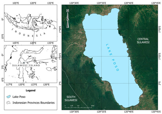
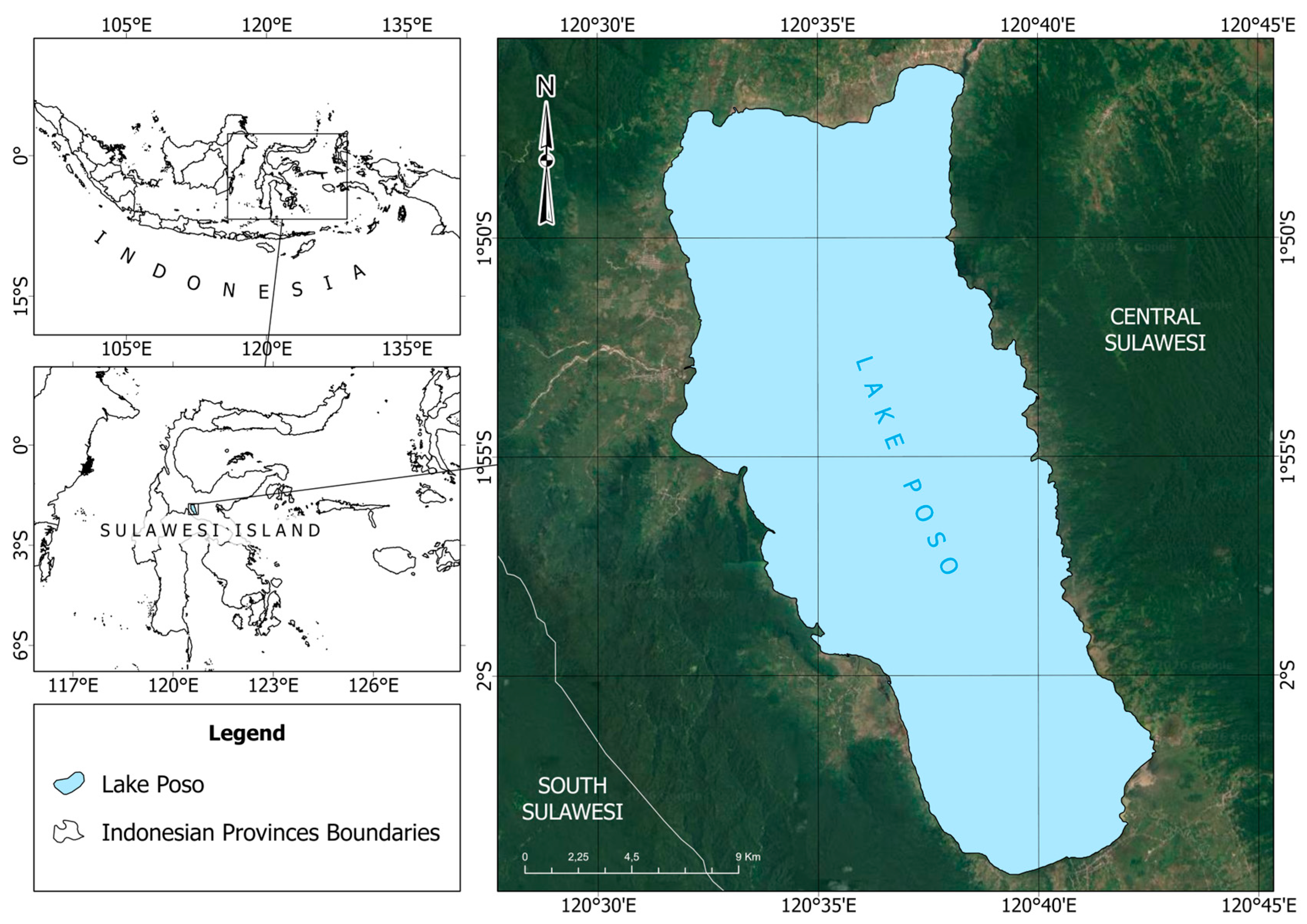
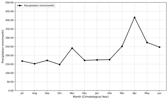
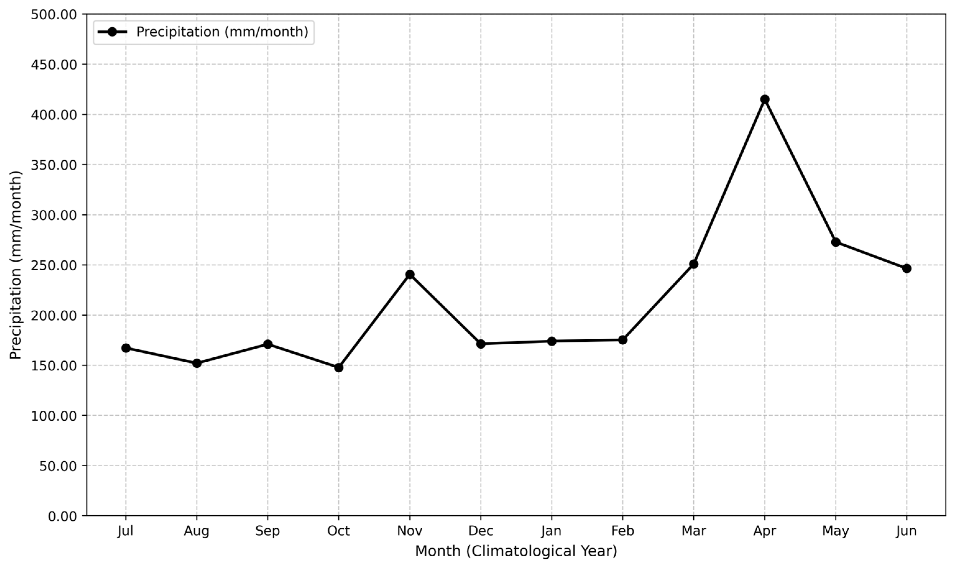
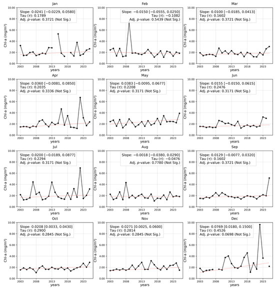
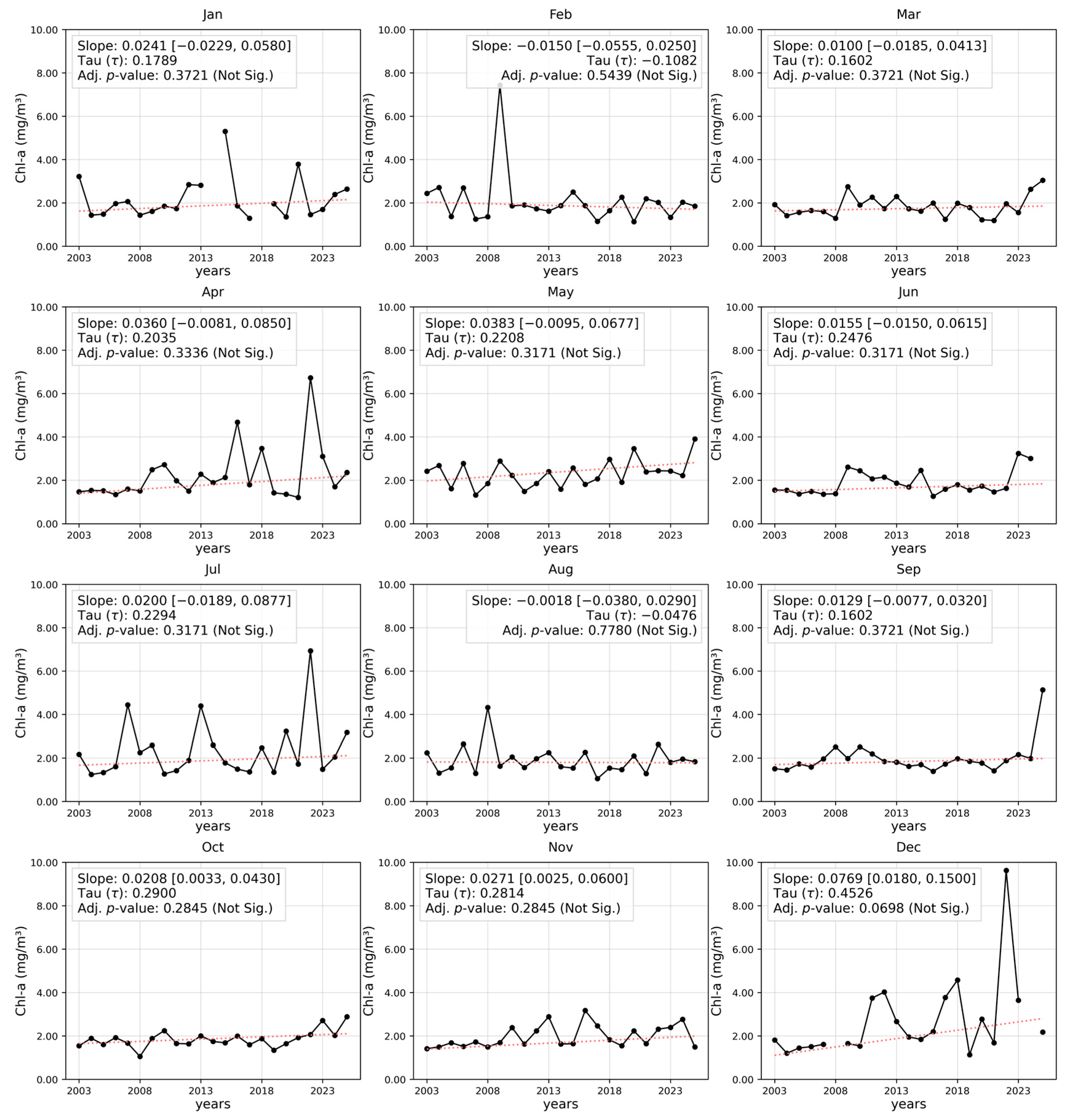
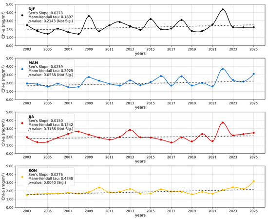
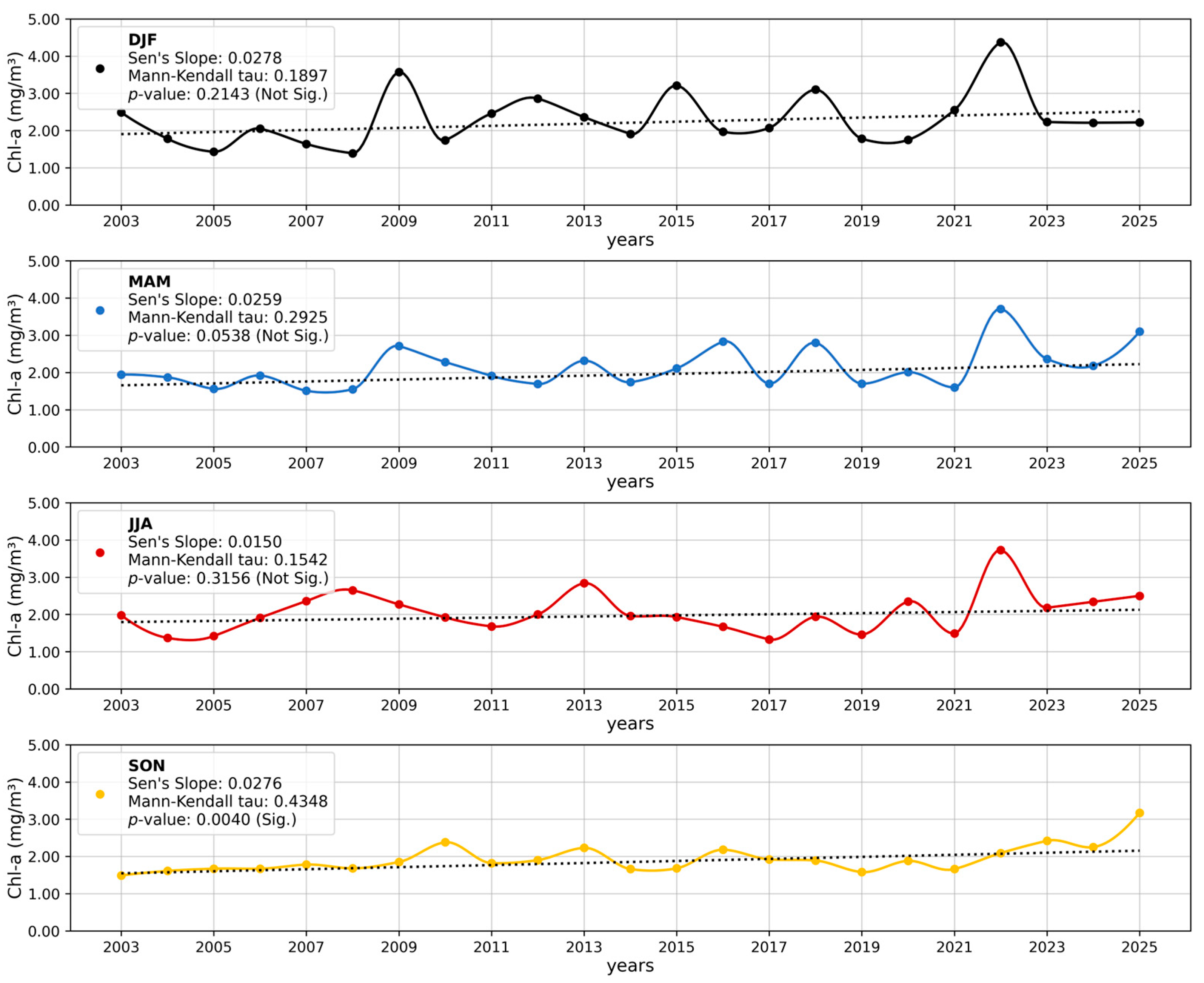
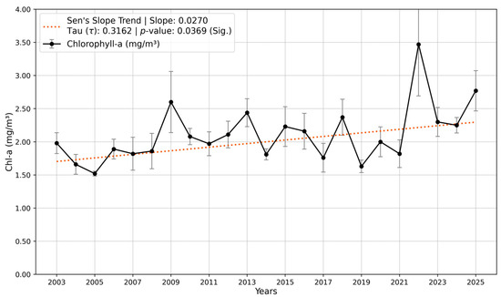
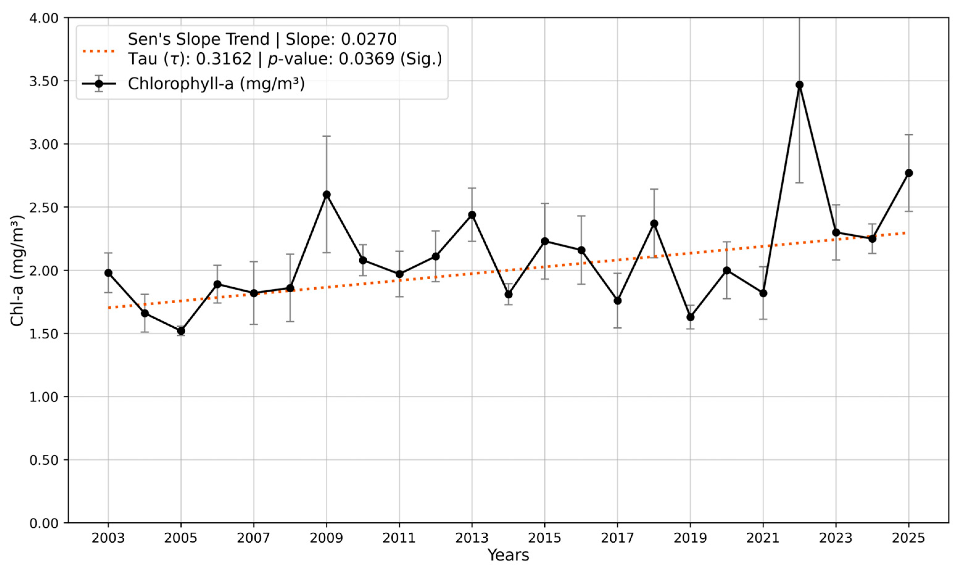
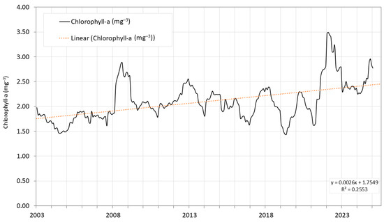
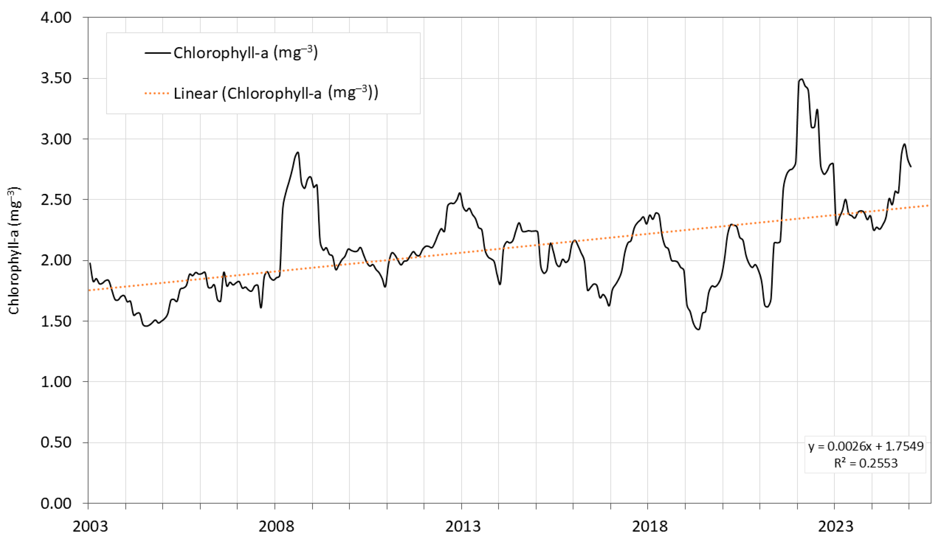
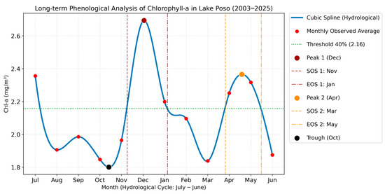
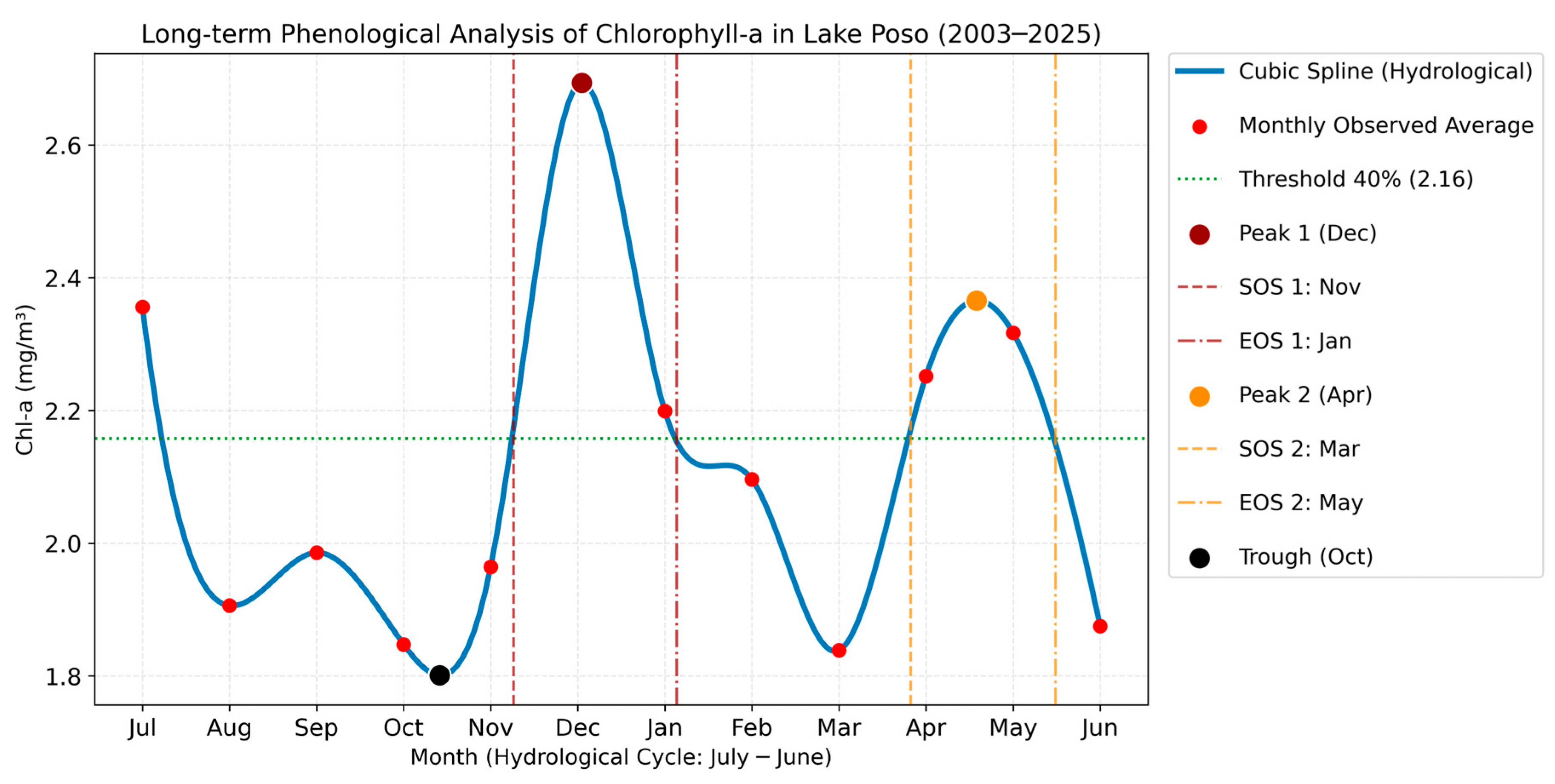
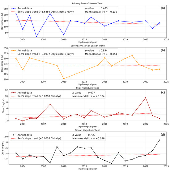
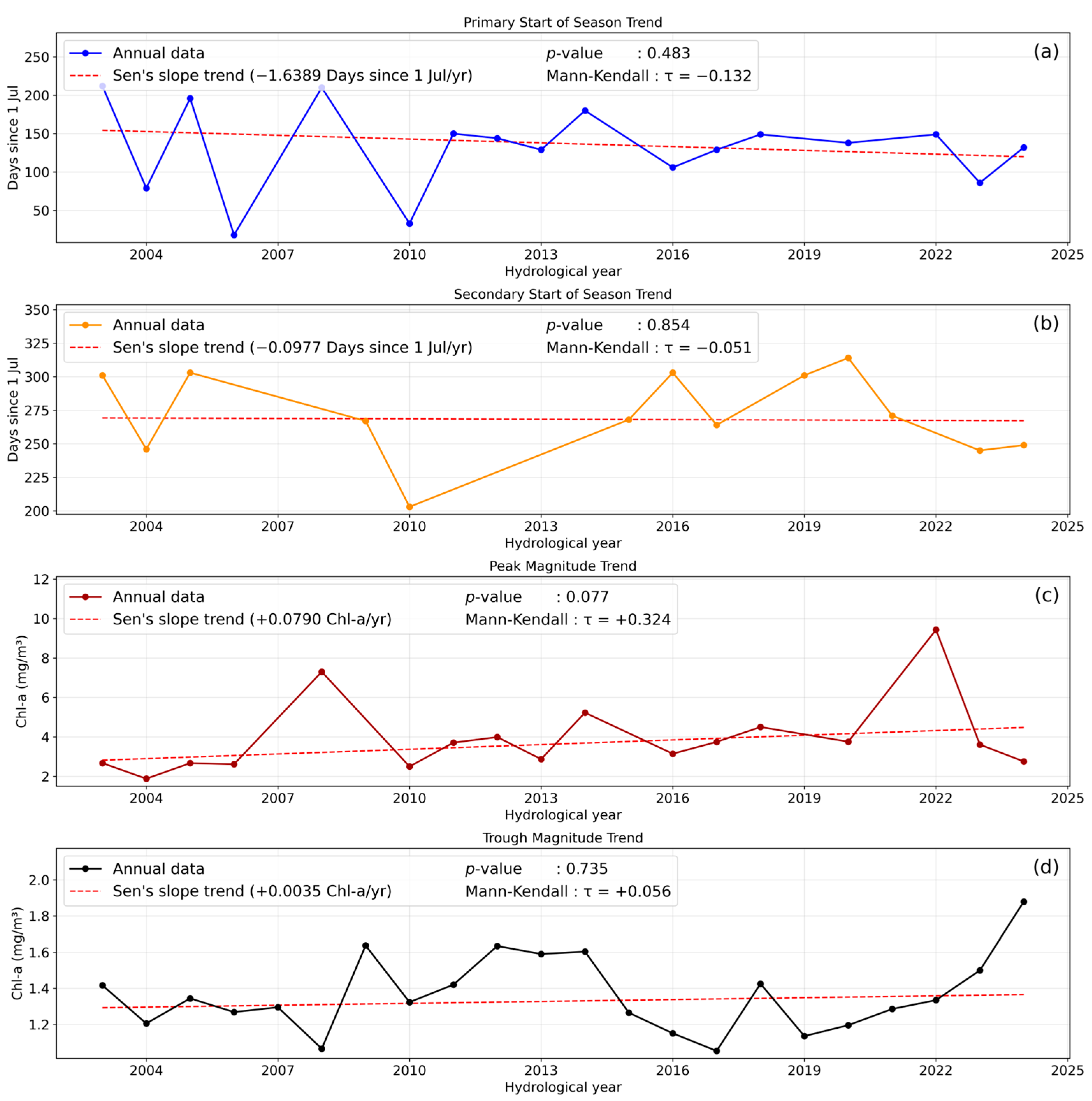
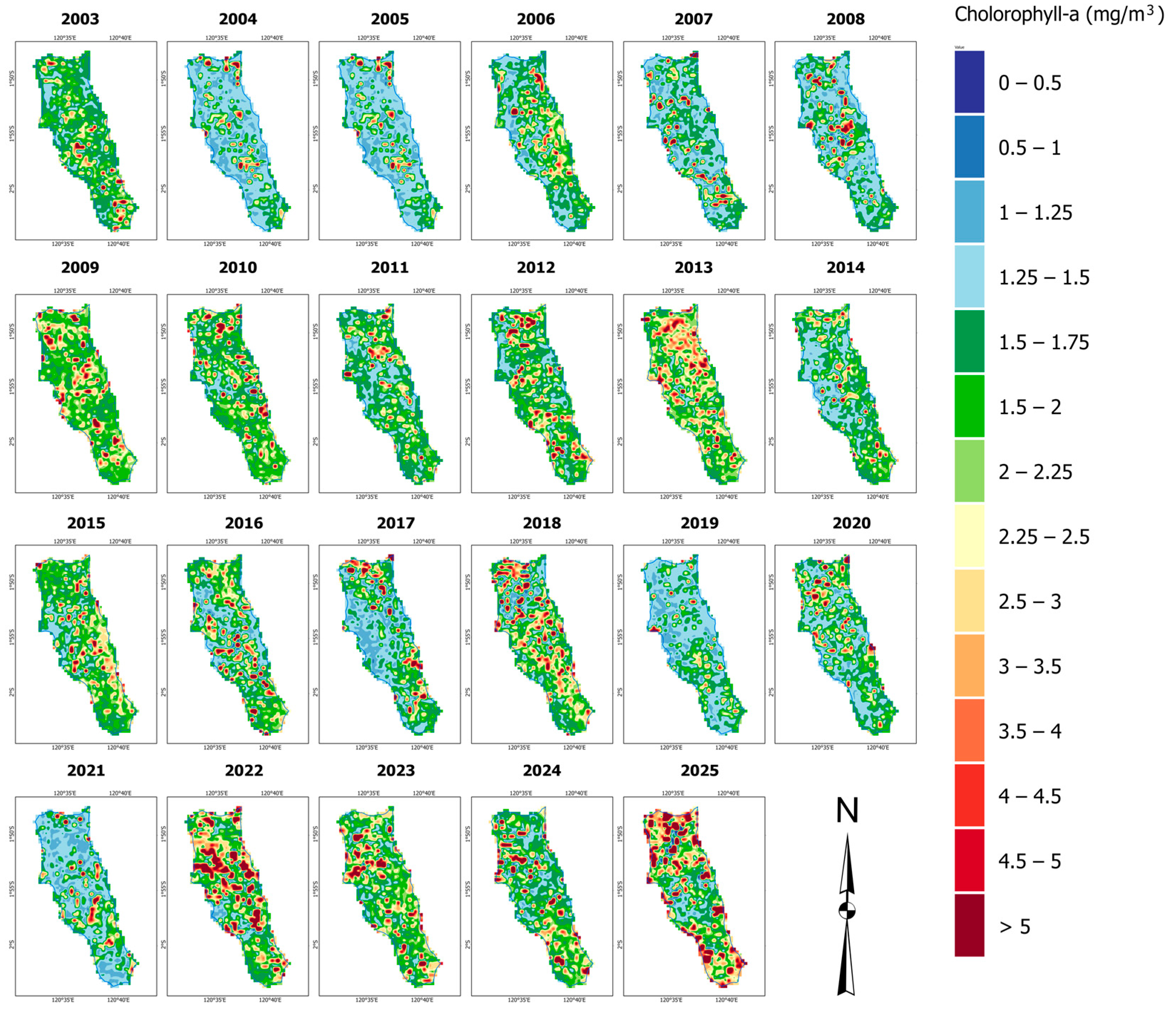
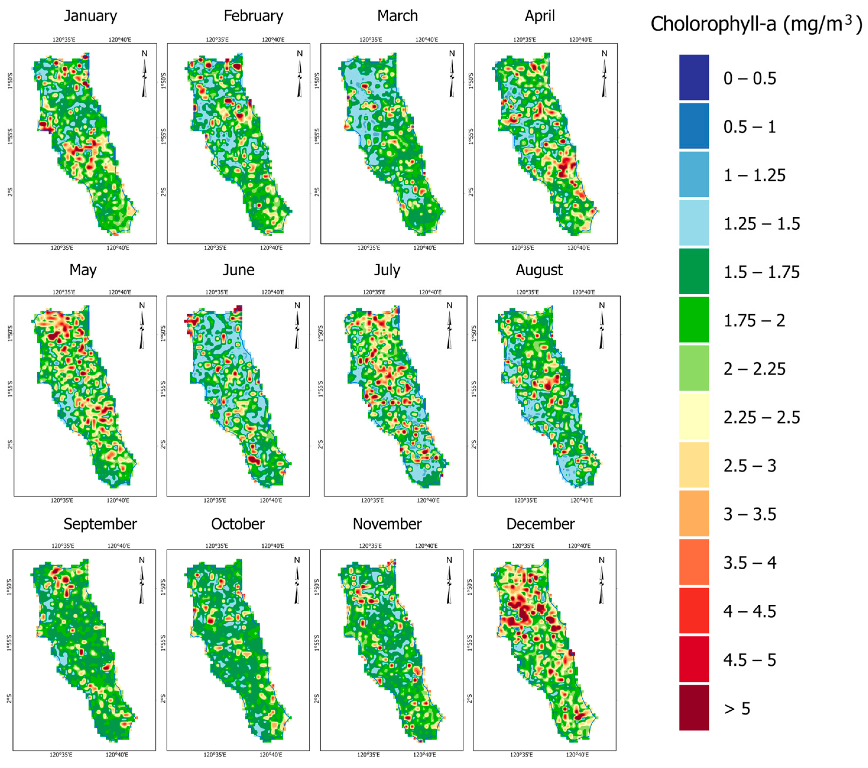
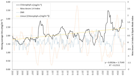
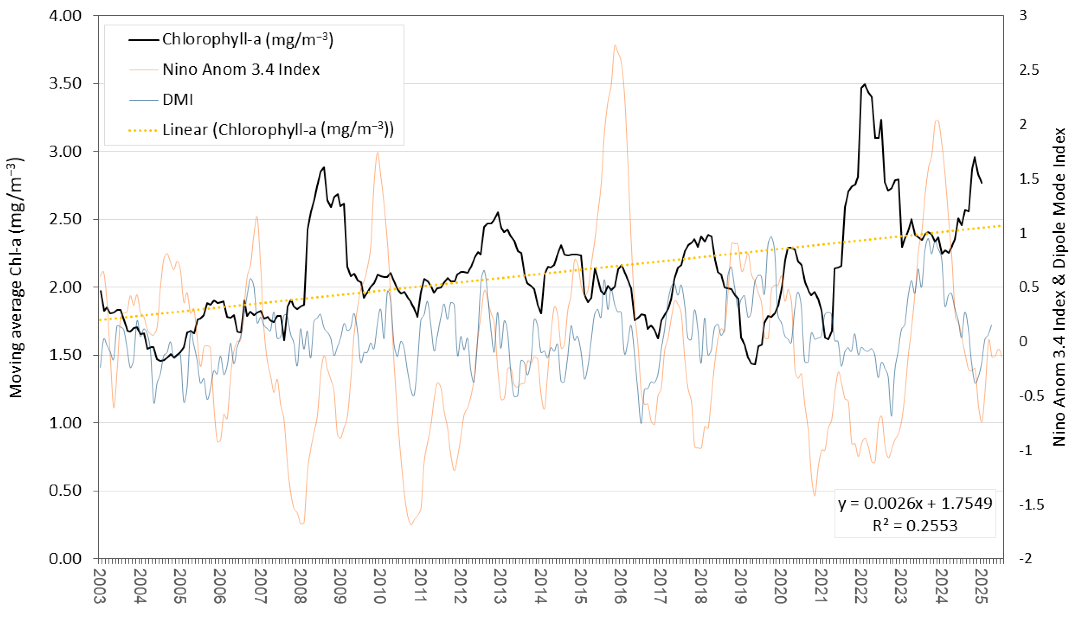
Disclaimer/Publisher’s Note: The statements, opinions and data contained in all publications are solely those of the individual author(s) and contributor(s) and not of MDPI and/or the editor(s). MDPI and/or the editor(s) disclaim responsibility for any injury to people or property resulting from any ideas, methods, instructions or products referred to in the content. |
© 2026 by the authors. Licensee MDPI, Basel, Switzerland. This article is an open access article distributed under the terms and conditions of the Creative Commons Attribution (CC BY) license.