


Abstract
We investigate a discretized two-dimensional tumor–immune model with a fractional-order-dependent step coefficient with seven effective parameters, where the fractional derivative with a piecewise constant argument is employed. The resulting model can possess one, two, or three equilibrium points, one of which is always unstable and corresponds to the malignant case, while the other two are stable under certain conditions. By applying the normal form method and bifurcation theory, we prove that the system undergoes a period-doubling bifurcation at one positive equilibrium point. The obtained bifurcation results provide a mathematical framework for exploring how changes in model parameters may affect the qualitative dynamics of tumor–immune interactions, including the emergence of oscillatory and potentially more complex dynamical regimes. Numerical simulations and visualizations are provided to illustrate these dynamical scenarios and to confirm the theoretical results.
1. Introduction
Cancer remains one of the leading causes of mortality worldwide, while many aspects of its initiation, progression, and response to treatment remain incompletely understood. Modern science recognizes that cancer development is not an isolated cellular process, but a dynamic and non-linear interaction between malignant cells and the host’s immune system, a phenomenon known as cancer immunoediting [1,2]. The high variability in patient clinical outcomes emphasizes the need for a more rigorous quantitative analysis of these interaction dynamics [3,4]. In this context, mathematics provides a theoretical framework to analyze, simulate, and predict tumor–immune dynamics that are otherwise challenging to capture through restrictive in vitro or in vivo experimental methods [3,5]. Historically, mathematical descriptions of tumor growth began as phenomenological frameworks focused exclusively on the population kinetics of cell growth without external microenvironmental influences. Classical frameworks, such as the Gompertz and logistic growth models, captured the initial exponential phase of tumor growth followed by a deceleration as a result of resource and spatial limitations. In 1994, Kuznetsov et al. formulated a model using a system of non-linear ordinary differential equations, treating the interaction between tumor cells and cytotoxic T-lymphocytes as an ecological predator–prey system [2]. That work mathematically formalized critical immunological phenomena, including immune surveillance, the “sneaking through” mechanism, and tumor dormancy [2]. A few years later, Kirschner and Panetta expanded this foundation by incorporating cytokine signaling, specifically interleukin-2, which successfully captured long-term oscillations and tumor relapse driven by immune feedback loops [6].
One of the earliest mathematical models describing interactions between tumor and immune cells was proposed by Stepanova in 1980 [7], in the form of a system of ordinary differential equations:
where represents the populations of the tumor cells, and reflects the activity or density of immunocompetent cells, such as T-cells, at time t. This model has been accepted as a basic model for tumor–immune system interaction because it contains many medically important features. In the literature, various versions of the system have been studied (1) with exponential [8], logistic [9,10] or generalized logistic function [11]. Many important studies devoted to the modeling, analysis, and control of tumor–immune system interactions can be found in [2,6,12,13,14]. Various authors have investigated the stability and bifurcation structures of modified Stepanova-type frameworks, highlighting how varying the immune response rates triggers transitions from controlled tumor dormancy to sudden escape regimes. To capture the intrinsic time required for immune cell maturation and recruitment, several researchers incorporated discrete time delays into the system. Khajanchi [15] proved that when these time delays exceed critical thresholds, the interaction dynamics undergo a Hopf bifurcation, eventually giving rise to highly unpredictable, deterministic chaotic attractors that mathematically represent long-term tumor relapse. Tumor growth takes place in a biologically heterogeneous microenvironment characterized by spatial variations in cellular composition, nutrient availability, oxygen supply, and interactions between tumor and immune cells. The importance of spatial heterogeneity for collective cellular dynamics has also been demonstrated in [16].
Extensions of classical integer-order models have been investigated to allow for a wider range of temporal responses and dynamical behaviors. The interaction between cancer and immune effector cells is explored in a mathematical model with a fractional operator, as described in the study [17]. Debbouche et al. [18] established that the proposed fractional-order cancer model exhibits chaotic dynamics in both commensurate and incommensurate cases.
The theory of fractional-order differential equations is still developing, while their applications have expanded to numerous scientific fields, including population dynamics, fluid mechanics, mechanics, physics, chemistry, finance, epidemiology, medicine, and engineering [19,20,21,22,23,24,25,26]. Several studies have demonstrated that fractional-order derivatives can provide a more flexible description of dynamical systems than corresponding classical models, particularly when systems exhibit complex responses across multiple time scales, anomalous transport, or memory and hereditary effects [27,28,29,30,31]. For example, in viscoelastic materials, the time-fractional derivative of strain can be incorporated into constitutive relations describing the experimentally observed relationship between stress and deformation. Such models have been investigated for soft biological tissues and tissue-mimicking materials, where classical integer-order models may not adequately reproduce the measured mechanical response over a broad range of frequencies [32]. Another important example is anomalous diffusion, in which the measured mean-squared displacement of particles may follow a power-law dependence on time, rather than the linear time dependence characteristic of classical Brownian diffusion. Time- and space-fractional differential operators are used to model such transport phenomena in complex and heterogeneous media [33,34]. These examples demonstrate that fractional calculus provides a modeling framework for describing measurable physical and biological phenomena that may involve nonlocal temporal or spatial dependencies.
Based on this motivation, the present study investigates a discretized tumor–immune interaction model derived from a fractional-order formulation, focusing on the conditions for period-doubling bifurcation and the resulting changes in the dynamical behavior of the system.
In [35], the authors extended the standard tumor–immune interaction model by replacing the integer-order dynamics with a fractional-order formulation. The fractional-order counterpart of model (1) is given by
where is the Caputo fractional operator defined as
j is the least integer which is not less than , and is the Riemann–Liouville integral operator of order , which is given by
Here, is Euler’s Gamma function. The term represents the exponential growth of the tumor cell population, assuming that the growth rate is proportional to the number of tumor cells present. This assumption is most appropriate at low cell densities, when competition for space and nutrients is negligible. As a result of the tumor–effector cell interaction, immune system cells cause elimination of cancer volume, which is given by the term in the first equation. In the second equation, the term represents the proliferation of lymphocytes due to stimulation by the anti-tumor antigen, which is in proportion to the tumor volume . However, large tumors inhibit the immune system’s activity, and this is reflected by incorporating the term into the model. Lymphocyte cells, like many other cells, possess an apoptosis mechanism that regulates the magnitude and duration of immune responses. This process occurring in immune system cells is roughly considered s the natural death rate and is mathematically represented by the term . The parameter represents the constant flow rate of immune system cells into the relevant tumor region.
In the numerical simulations in this paper we use some parameters values given in Table 1 which are estimated in [2] and used in many papers [11,35,36].
Table 1.
Numerical values for the parameters used in simulations.
To investigate chaotic behavior, which represents one of the important features of tumor dynamics, in the considered two-dimensional dynamical system, it is necessary to transform Equation (2) into a system of difference equations. For this purpose, several studies [19,23,29,35,37] have developed approaches for obtaining explicit difference equations by applying discretization techniques based on piecewise constant arguments as follows. Assume that and are the initial conditions of system (2). The discretization of system (2) with piecewise constant arguments is given as
If , then . Thus, we obtain
The solution of system (5) is
That is,
Repeating this process, the solution of system (1) is obtained as
This leads to the following system of difference equations:
In this model, the fractional-order parameter is structurally embedded within the scaling step-size operator, defined as . This formulation acts as a hybrid phenomenological framework that introduces a non-linear time transformation.
Authors in [35] derived the conditions for the occurrence of a Neimark–Sacker bifurcation. In this paper, we complement their analysis by investigating the existence of period-doubling bifurcations, an intriguing phenomenon that has attracted considerable attention from both mathematical and biological perspectives and has been extensively studied by various authors; see [38,39], and the onset of chaos associated with the period-doubling mechanism. From a therapeutic perspective, the identification of period-doubling bifurcations may be relevant for understanding how changes in biological or treatment-related parameters can affect the long-term behavior of tumor cell populations. The transition from stable to oscillatory and potentially chaotic dynamics may indicate a loss of predictability in tumor evolution, which can complicate the assessment of treatment response. Therefore, identifying parameter regimes associated with stable or complex dynamics may provide a theoretical basis for investigating how therapeutic interventions could influence the qualitative behavior of tumor growth. Although such results do not directly imply clinical treatment strategies, they can contribute to the mathematical understanding of tumor dynamics and provide a framework for exploring treatment scenarios through further modeling and numerical analysis.
The rest of this paper is organized as follows. Section 2 presents the stability analysis of the fixed points of the discrete system. Section 3 is devoted to the analysis of period-doubling bifurcations and the resulting chaotic dynamics. Finally, Section 4 presents numerical simulations that validate the theoretical results. All visualizations are generated using Mathematica, Wolfram, and Dynamica 3.0 [40]. We also calculated Lyapunov exponents by using the computational algorithm in [41] since it is a tool for determining the sensitivity to minor disturbances of the initial conditions, so that if the maximum value of LE is positive, chaotic behavior is seen, if the maximum value of LE is zero, periodic behavior is seen, and if the maximum value of LE is negative, the fixed-point is observed.
2. Equilibrium Points and Their Local Stability
In this section, we determine the equilibrium points of the system (8) by solving the following equations.
From the first equation, it follows that If , the second equation implies and since , tumor-free equilibrium always exists. If , then replacing in the second equation, we obtain
which implies
Mathematically, the equilibrium points exist if and only if the expression under the square root is non-negative. However, from a biological standpoint, it is essential that the equilibria, or their components, are non-negative. Hence, we distinguish the following scenarios:
Let us denote the above-mentioned conditions as
and
To investigate the local stability of the positive equilibrium point, we apply Lemma A1 and Theorem A1 (see Appendix A), which provide stability criteria in terms of the moduli of the eigenvalues of the Jacobian matrix evaluated at the equilibrium point.
Theorem 1.
- (a)
- Locally asymptotically stable if
- (b)
- Nonhyperbolic point if
- (c)
- A saddle point ifor
- (d)
- A repeller if
Proof.
By evaluating the Jacobian of system (8) at the equilibrium point we obtain
The eigenvalues are
If , then i.e., . If and , then . Hence, the equilibrium point is locally asymptotically stable. The rest of the proof follows analogously. □
Theorem 2.
Equilibrium point is a nonhyperbolic point.
Proof.
Since the Jacobian matrix is of the form for , it implies that and . Further,
□
Theorem 3.
Proof.
The Jacobian of the system (8) at the equilibrium point is of the form
The Jacobian matrix of the system (8) at the equilibrium point is of the form
Further, let us check when condition (iii) in Theorem A1 is satisfied. Since
considering conditions (11) and (12), it implies if
This proves the following theorem.
3. Period-Doubling Bifurcation
In this section we analyse when the equilibrium point of system (8) undergoes period-doubling bifurcation. This type of bifurcation occurs if the system possesses one eigenvalue equal to −1 and the other satisfies the condition . Let us introduce the following notations in order to simplify the calculus: , and .
In order to obtain period-doubling bifurcation, it must hold and . Since it implies . Hence, . Let us define the curve where exists period-doubling bifurcation:
where
Notice
Let us convert the system (8) into the system with equilibrium point at the origin by using the translation
Hence, we obtain
We will henceforth use the following Taylor expansion
where , , and denote the corresponding coefficients in the Taylor expansion.
Let us transform the system (20) in
Suppose that In order to make the normal form of system (20), we consider invertible matrix
where , , . So, we get
Taking into account the following similarity transformation
system takes the form
Further, it holds
where
and
It implies
After tedious calculations, we obtain
where
i.e.,
Using the expansion in (21), we obtain
and
where coefficients and , are given in Appendix A. Due to center manifold theory [42], stability analysis of equilibrium near can be discussed by investigating reduced equations on a center manifold
We assume that the center manifold can be approximated by
where , , , , , , , , , , , and are unknown coefficients. Since it must hold
we get
where coefficients , , , , , , , , , , , and are given in Appendix A. Further, it holds
so the center manifold can be described as follows
where . Now, we restrict our system to the center manifold
It holds
Using the coefficient in the expansion (21), which is given by
, and we get
and
So,
and
where
Now we have,
If the discriminant of the quadratic equation is negative, then . If , then there are two positive solutions given by
So,
Since for we have that
Based on the period doubling bifurcation theorem in [43], the three following conditions must be satisfied:
- (i)
- (ii)
- and
- (iii)
- , if or and , where is discriminant of the quadratic equation with respect to where is given by (22).
We have thus proved the following theorem:
4. Numerical Results
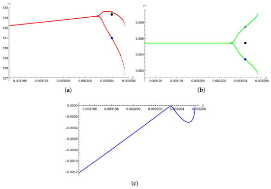
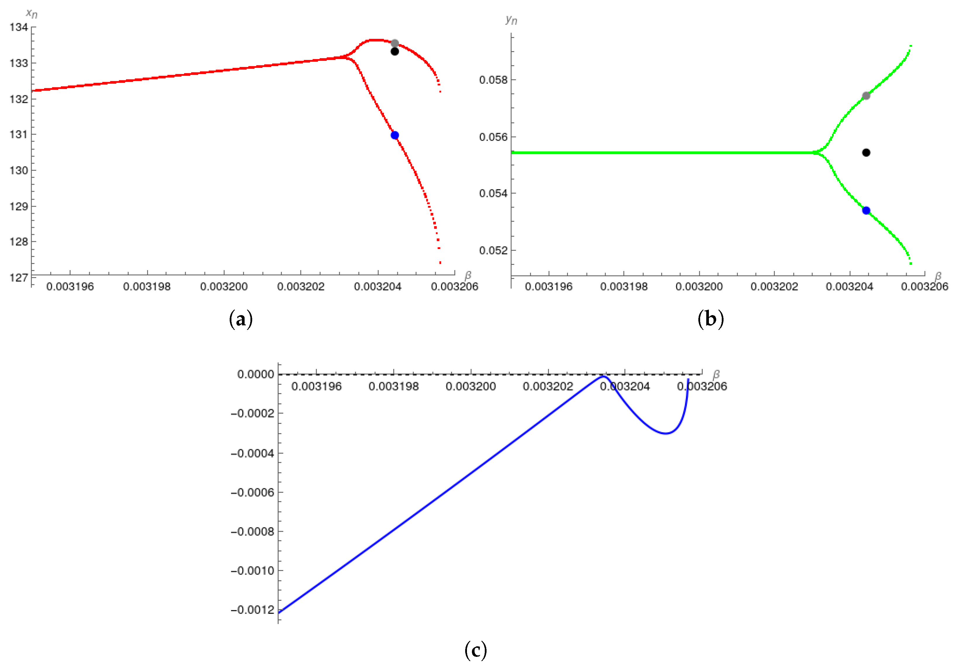
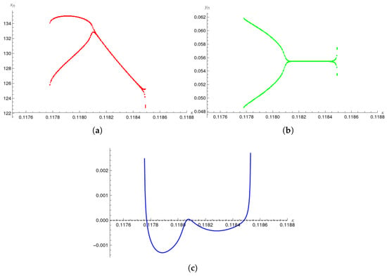
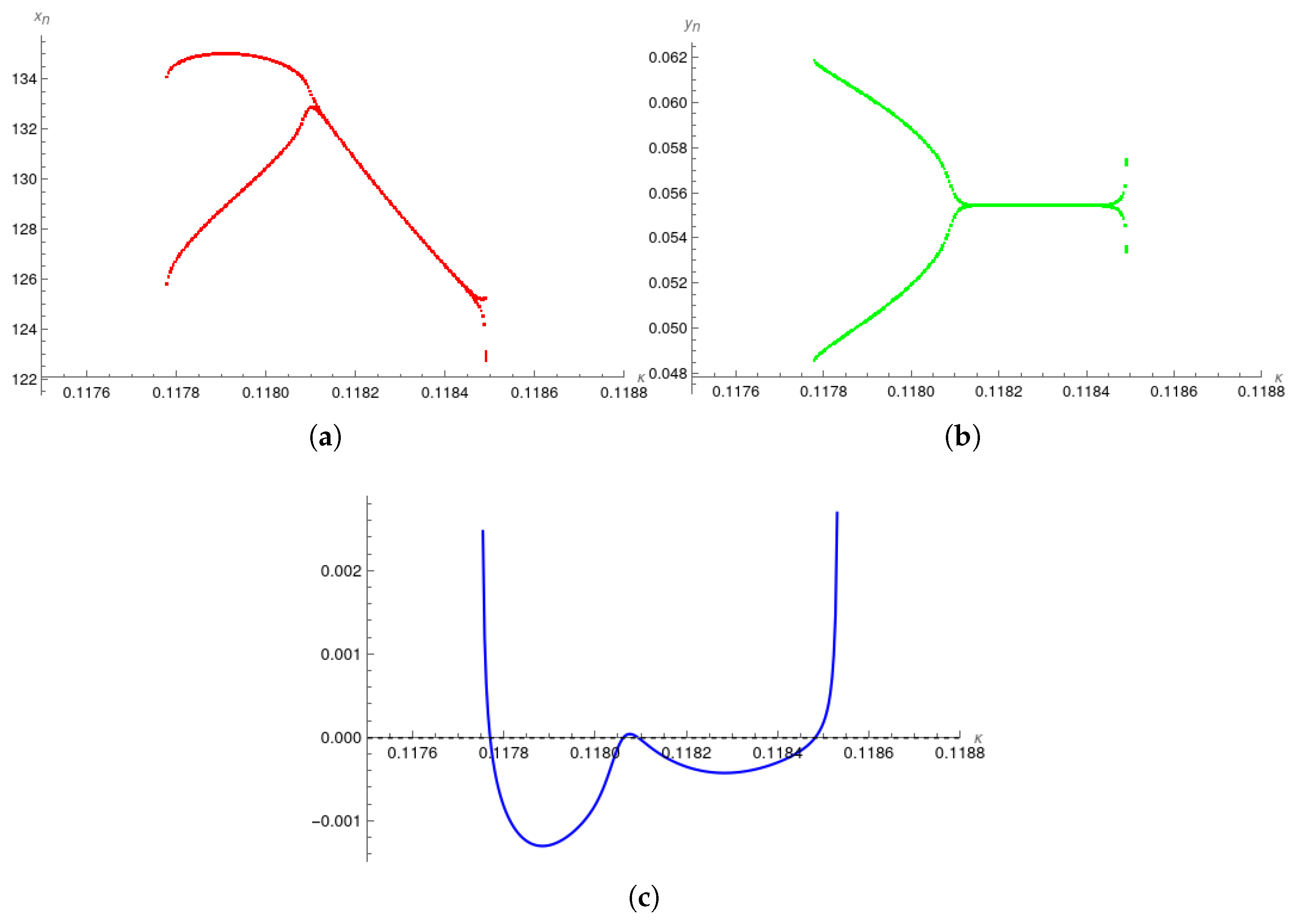
For the selected parameter values , and , the critical value of the parameter corresponding to the period-doubling bifurcation is obtained from (18) as . At , the Jacobian matrix evaluated at the equilibrium point of system (8) has eigenvalues and , confirming the eigenvalue condition for the occurrence of a period-doubling bifurcation. Further, the non-degeneracy condition (iii) holds because . Hence, all the assumptions required for the existence of a period-doubling bifurcation at the equilibrium point are satisfied. Since , the corresponding bifurcation is supercritical period-doubling bifurcation of the tumor and immune effector cell population model, induced by increasing the inverse threshold for the tumor suppression parameter ; see Figure 1.
Figure 1.
(a,b) Bifurcation diagram for variables and , respectively, and values of parameters , , , , , , and initial conditions . Period-two solutions are (blue point) and (gray point) for parameter value . The equilibrium point is (black point). (c) Corresponding Lyapunov exponent for the same value of parameters.
For the selected parameter values and with initial condition , the dynamics of the tumor–immune system are governed by the variation of the inverse threshold tumor-suppression parameter . For , the system approaches a stable equilibrium, corresponding to a stable level of both populations. At , the equilibrium loses stability through a period-doubling bifurcation and a stable period-two solution emerges; see Figure 1. From a biomedical perspective, a supercritical period-doubling bifurcation provides a mathematical framework for investigating how changes in model parameters may lead to qualitative changes in the dynamics of a tumor–immune system. In particular, the emergence of a stable period-two orbit in the discrete model indicates the possibility of alternating states within the mathematical description. The identified bifurcation mechanism may serve as a starting point for further investigations into the sensitivity of tumor–immune dynamics to parameter variations and the potential relevance of discrete-time effects. Establishing any biomedical significance would require validation against experimental or clinical data, biologically justified parameter estimates, and an assessment of whether the predicted trajectories remain within physiologically meaningful ranges. Thus, the present results provide a theoretical framework for future model-based studies.
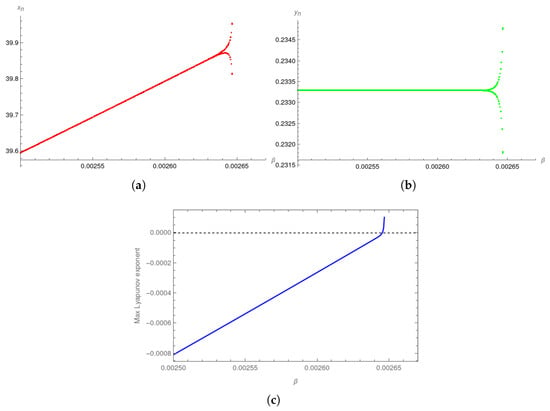
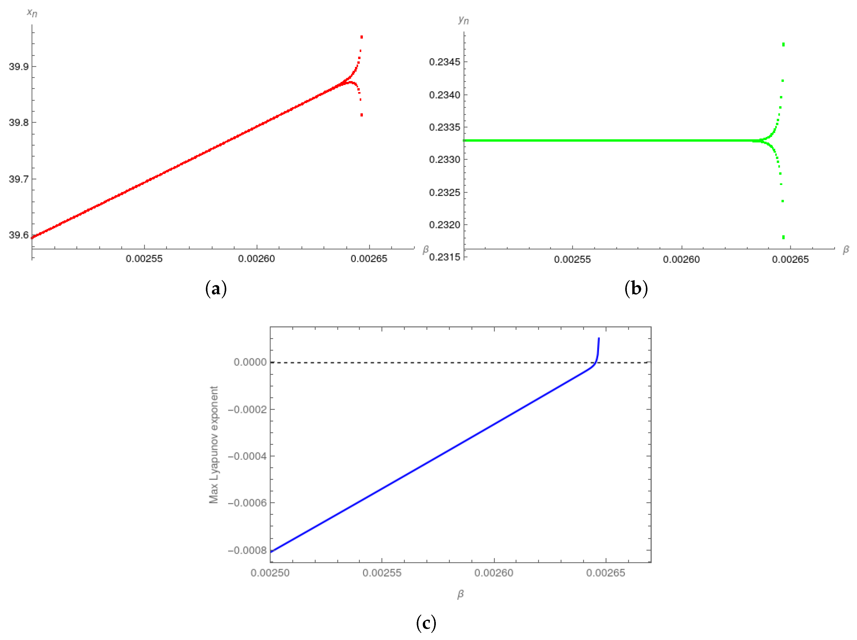
For the fixed parameter values , , , , , with fractional order and discretization step , the critical value of the bifurcation parameter is . The eigenvalues of the Jacobian matrix evaluated at the equilibrium point are and . The nondegeneracy condition is now . Therefore, the period-doubling bifurcation is subcritical; see Figure 2. The associated period-two orbit is unstable and does not attract nearby trajectories.
Figure 2.
(a,b) Bifurcation diagram for variables and , respectively, and values of parameters , , , , , , and initial conditions . (c) Corresponding Lyapunov exponent for the same value of parameters.
Figure 3 illustrates the dependence of the discretized tumor–immune system dynamics on the immune–cell influx parameter in the case when supercritical bifurcation occurs. The bifurcation diagrams for and indicate changes in the structure of the observed dynamical branches near two values and . The observed changes suggest that the immune-cell influx parameter can have a substantial effect on the dynamics of the model.
Figure 3.
(a,b) Bifurcation diagram for variables and , respectively, and values of parameters , , , , , , and initial conditions . (c) Corresponding Lyapunov exponent for the same value of parameters.
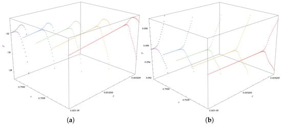
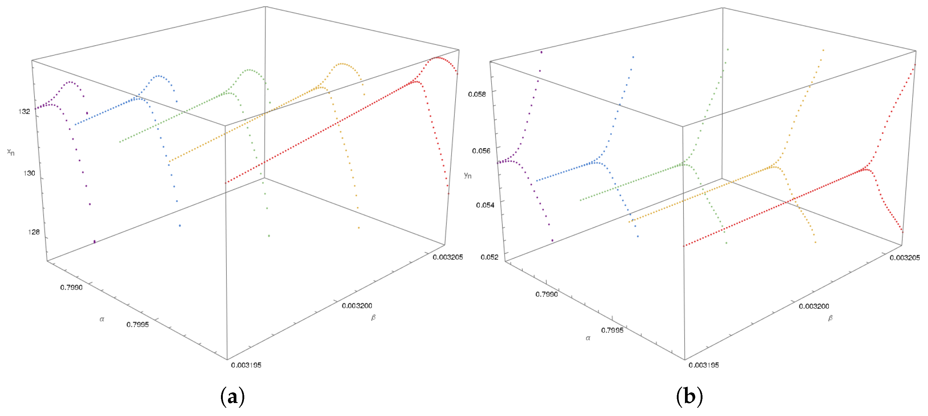
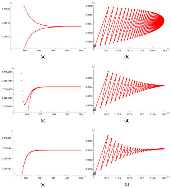
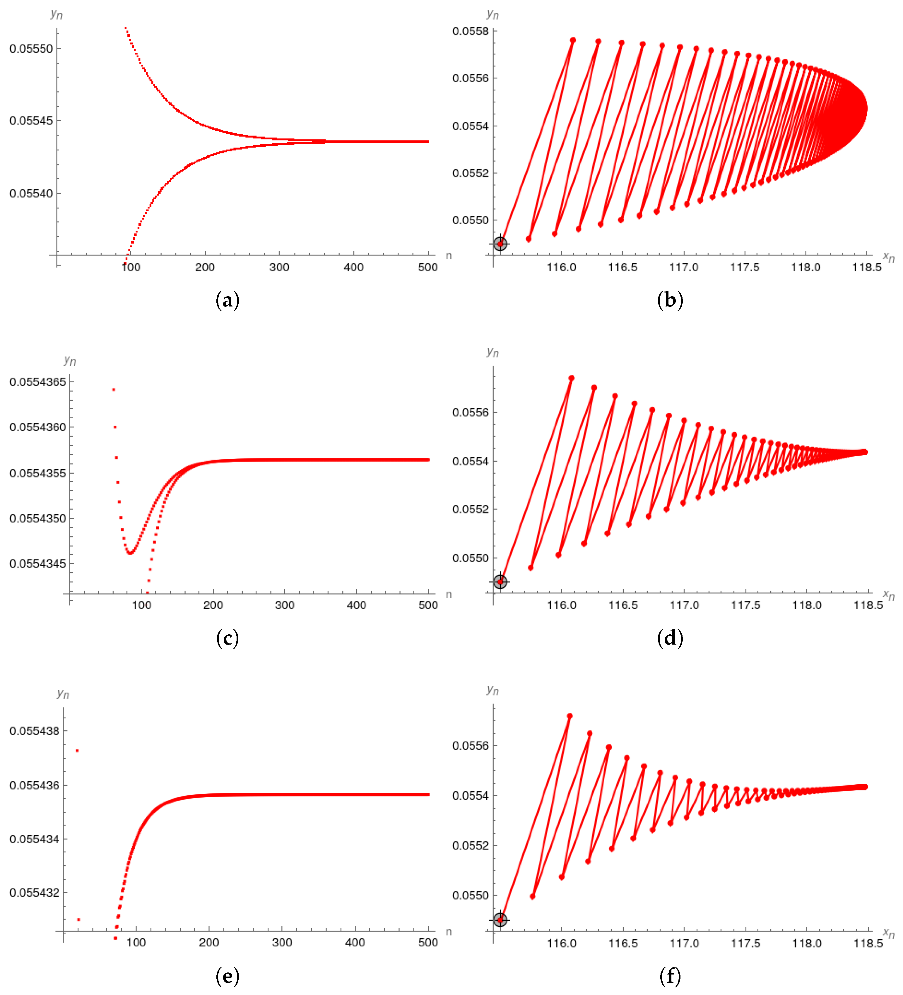
Figure 4 presents the bifurcation diagrams of the model with respect to the fractional-order parameter for different values of the parameter , illustrating how variations in these parameters affect the stability regions. A similar influence of parameter variations can also be observed in the corresponding orbit plots and phase portraits presented in Figure 5.
Figure 4.
(a,b) Bifurcation diagrams for variables and , respectively and values of parameters , , , , , , initial conditions and {0.79865, 0.798975, 0.799305, 0.79964, 0.799981}.
Figure 5.
Orbit plot and phase portraits for value of parameters , , , , , , and initial conditions and in (a,b), in (c,d) and in (e,f).
5. Discussion
In this study, we investigated the dynamical behavior of a discrete tumor–immune system model obtained from the fractional-order formulation of the Stepanova tumor model by using a discretization procedure with piecewise constant arguments. The model incorporates the interaction between tumor cells and immune effector cells, while the fractional-order formulation allows much more compatibility with real data. In contrast to previous studies of the considered model, where complex dynamics were mainly associated with the Neimark–Sacker bifurcation, the present study focuses on the occurrence of a period-doubling bifurcation and the resulting transition toward more complicated oscillatory dynamics.
The system can possess one, two, or three equilibrium points , and , which are called the tumor-free equilibrium point, malignant equilibrium point, and benign equilibrium point, respectively. The equilibrium point is always unstable, while the discrete-time dynamical system exhibits very complex dynamic behaviors around the equilibrium point . The local stability analysis of the equilibrium point shows that the stability of the tumor–immune system strongly depends on the model parameters. In particular, as the bifurcation parameter is varied, the eigenvalues of the linearized system change in such a way that one eigenvalue reaches the critical value . This provides the mathematical mechanism for the occurrence of a period-doubling bifurcation. At the critical parameter value, the stable equilibrium loses its stability and a period-two orbit emerges. Thus, the observed numerical transition is not merely a numerical phenomenon, but is supported by the analytical bifurcation conditions obtained for the discrete system.
The bifurcation diagram further illustrates the evolution of the tumor dynamics as the selected parameter increases. Before the critical value, the tumor–immune system approaches a stable equilibrium, corresponding to a regular long-term behavior of the tumor and immune-cell populations. After the critical value, the system exhibits periodic oscillations of period two. With a further variation of the parameter, successive period-doubling transitions may occur, leading to higher-period oscillations and eventually to irregular or chaotic behavior. This demonstrates that relatively small changes in biologically relevant parameters can substantially modify the long-term behavior predicted by the model.
From a biological point of view, the appearance of period-doubling dynamics may be interpreted as a transition from a stable tumor–immune interaction to an oscillatory regime in which tumor cells and immune effector cells repeatedly change their population levels. Such behavior may reflect alternating phases of tumor growth and immune response. Although the mathematical model cannot directly predict a specific clinical outcome, the existence of bifurcation points indicates parameter regimes in which the system becomes particularly sensitive to changes in biological or treatment-related parameters. Therefore, identifying these critical thresholds may be useful for understanding transitions between stable, periodic, and potentially irregular tumor dynamics.
The results also complement the findings obtained for the same tumor–immune model in previous studies. While the Neimark–Sacker bifurcation describes a loss of stability associated with the appearance of quasiperiodic dynamics, the present analysis demonstrates that the same model can also undergo a period-doubling bifurcation through a real eigenvalue crossing . Consequently, different parameter regimes can generate qualitatively different routes toward complex dynamics. This highlights the importance of considering more than one bifurcation mechanism when analyzing discrete tumor–immune models.
Author Contributions
Conceptualization, S.H. and S.M.; methodology, S.H., S.M. and Z.N.; software, S.H., S.M. and Z.N.; validation, S.H., S.M. and Z.N.; formal analysis, S.H., S.M. and Z.N.; investigation, S.H., S.M. and Z.N.; resources, S.H., S.M. and Z.N.; writing—original draft preparation, S.H., S.M. and Z.N.; writing—review and editing, S.H., S.M. and Z.N.; visualization, S.H., S.M. and Z.N.; project administration, S.H. All authors have read and agreed to the published version of the manuscript.
Funding
This work was supported by the Ministry of Education and Science of Tuzla Canton, Bosnia and Herzegovina under Grant No. 10/1-11-13096-2/26 dated 25 June 2026.
Data Availability Statement
All data and parameters generated or analyzed during this study are included in this published article.
Acknowledgments
The authors would like to thank the anonymous reviewers for their valuable comments and suggestions, which helped to improve the quality and presentation of this manuscript.
Conflicts of Interest
The authors declare no conflicts of interest.
Appendix A
Lemma A1
([44]). Assume that is a polynomial associated with the characteristic equation. Suppose that , and and are two roots of . Then,
- (a)
- and iff and .
- (b)
- and iff and
- (c)
- and (or and ) iff .
- (d)
- and are complex and iff and .
- (e)
- and iff and ,
- (f)
- iff and .
Recall now some definitions of topological types for an equilibrium point . If and , an equilibrium point is called a sink. As we know, a sink is locally asymptotically stable. If and , an equilibrium point is called a locally unstable source. If and (or and ) an equilibrium point is called a saddle. And, finally, if either or , an equilibrium point is called non-hyperbolic.
Theorem A1.
The zeros of the characteristic polynomial
lie inside the unit disk if and only if the following conditions hold:
- (i)
- ;
- (ii)
- ;
- (iii)
- .
Appendix A.1. Coefficients of the Functions f and g
Appendix A.2. Coefficients of the Center Manifold
References
- Mahlbacher, G.E.; Reihmer, K.C.; Frieboes, H.B. Mathematical modelling of tumor-immune cell interactions. J. Theor. Biol. 2019, 469, 47–60. [Google Scholar] [CrossRef] [Scilit] [PubMed]
- Kuznetsov, V.; Makalkin, I.A.; Taylor, M.A.; Perelson, A. Nonlinear dynamics of immunogenic tumors: Parameter estimation and global bifurcation analysis. Bull. Math. Biol. 1994, 56, 295–321. [Google Scholar] [CrossRef] [Scilit] [PubMed]
- Altrock, P.M.; Liu, L.L.; Michor, F. The mathematics of cancer: Integrating quantitative models. Nat. Rev. Cancer 2015, 15, 730–745. [Google Scholar] [CrossRef] [Scilit] [PubMed]
- Eftimie, R.; Bramson, J.L.; Chaplain, M.A. Mathematical modelling of immunotherapies for cancer. Philos. Trans. R. Soc. A 2011, 369, 4139–4171. [Google Scholar]
- de Pillis, L.G.; Radunskaya, A.E.; Wiseman, C.L. A valid mathematical model of cell-mediated immune response to tumor growth. Cancer Res. 2005, 65, 7950–7958. [Google Scholar] [CrossRef] [Scilit] [PubMed]
- Kirschner, D.; Panetta, J.C. Modeling immunotherapy of the tumor-immune system interaction. J. Math. Biol. 1998, 37, 235–252. [Google Scholar]
- Stepanova, N. Course of the immune reaction during the development of a malignant tumor. Biophysics 1980, 24, 917–923. [Google Scholar]
- Vladar, H.P.; González, J.A. Dynamic response of cancer under the influence of immunological activity and therapy. J. Theor. Biol. 2004, 227, 335–348. [Google Scholar] [CrossRef] [Scilit] [PubMed]
- Dassow, M.; Djouadi, S.; K. Moussa, K. Optimal control of a tumor-immune system with a modified stepanova cancer model. IFAC-PapersOnLine 2021, 54, 227–232. [Google Scholar] [CrossRef] [Scilit]
- Moussa, K.; Fiacchini, M.; Alamir, M. Robust optimal scheduling of combined chemo- and immunotherapy: Considerations on chemotherapy detrimental effects. In Proceedings of the American Control Conference (ACC), Denver, CO, USA, 1–3 July 2020; pp. 4252–4257. [Google Scholar] [CrossRef] [Scilit]
- Ledzewicz, U.; Olumoye, O.; Schättler, H. On optimal chemotherapy with a strongly targeted agent for a model of tumor-immune system interactions with generalized logistic growth. Math. Biosci. Eng. 2013, 10, 787–802. [Google Scholar] [CrossRef] [Scilit] [PubMed]
- Foryś, Marchuk’s model of immune system dynamics with application to tumour growth. J. Theor. Med. 2002, 4, 85–93. [Google Scholar] [CrossRef] [Scilit]
- Mayer, H.; Zanker, K.S.; der Heiden, U. A basic mathematical model of the immune response. Chaos 1995, 5, 155–161. [Google Scholar] [CrossRef] [Scilit] [PubMed]
- Waniewski, J.; Zhivkov, P. A simple mathematical model for tumor-immune system interactions. In Proceedings of the Eighth National Conference on Application of Mathematics in Biology and Medicine, Lajs, Poland, 24–27 September 2002; pp. 149–154. [Google Scholar]
- Khajanchi, S. Chaotic dynamics of a delayed tumor-immune interaction model. Int. J. Biomath. 2020, 13, 2050009. [Google Scholar] [CrossRef] [Scilit]
- Kindler, O.; Pulkkinen, O.; Cherstvy, A.G.; Metzler, R. Burst statistics in an early biofilm quorum sensing model: The role of spatial colony-growth heterogeneity. Sci. Rep. 2019, 9, 12077. [Google Scholar] [CrossRef] [Scilit] [PubMed]
- Kumar, S.; Kumar, A.; Samet, B.; Gómez-Aguilar, J.F.; Osman, M.S. A chaos study of tumor and effector cells in fractional tumor-immune model for cancer treatment. Chaos Solitons Fractals 2020, 141, 110321. [Google Scholar] [CrossRef] [Scilit]
- Debbouche, N.; Ouannas, A.; Grassi, G.; Al-Hussein, A.-B.A.; Tahir, F.R.; Saad, K.M.; Jahanshahi, H.; Aly, A.A. Chaos in cancer tumor growth model with commensurate and incommensurate fractional-order derivatives. Comput. Math. Methods 2022, 2022, 5227503. [Google Scholar] [CrossRef] [Scilit] [PubMed]
- Agarwal, R.P.; El-Sayed, A.M.A.; Salman, S.M. Fractional-order Chua’s system: Discretization, bifurcation and chaos. Adv. Differ. Equ. 2013, 2013, 320. [Google Scholar] [CrossRef] [Scilit]
- Arenas, A.J.; González-Parra, G.; Chen-Charpentier, B.M. Construction of nonstandard finite difference schemes for the SI and SIR epidemic models of fractional order. Math. Comput. Simul. 2016, 121, 48–63. [Google Scholar] [CrossRef] [Scilit]
- González-Parra, G.; Arenas, A.J.; Chen-Charpentier, B.M. A fractional order epidemic model for the simulation of outbreaks of influenza A (H1N1). Math. Methods Appl. Sci. 2014, 37, 2218–2226. [Google Scholar] [CrossRef] [Scilit]
- Laskin, N. Fractional Schrödinger equation. Phys. Rev. E 2002, 66, 056108. [Google Scholar] [CrossRef] [Scilit] [PubMed]
- Matouk, A.E.; Elsadany, A.A. Dynamical behaviors of fractional-order Lotka–Volterra predator–prey model and its discretization. J. Appl. Math. Comput. 2014, 49, 269–283. [Google Scholar] [CrossRef] [Scilit]
- Tarasov, V.E. Fractional vector calculus and fractional Maxwell’s equations. Ann. Phys. 2008, 323, 2756–2778. [Google Scholar] [CrossRef] [Scilit]
- Thamareerat, N.; Luadsong, A.; Aschariyaphotha, N. Stability results of a fractional model for unsteady-state fluid flow problem. Adv. Differ. Equ. 2017, 2017, 74. [Google Scholar] [CrossRef] [Scilit]
- Yuste, S.B.; Acedo, L.; Lindenberg, K. Subdiffusion-limited A+B → C reaction-subdiffusion process. Phys. Rev. E 2004, 69, 036126. [Google Scholar] [CrossRef] [Scilit] [PubMed]
- Jun, D.; Guang-jun, Z.; Yong, X.; Hong, Y.; Jue, W. Dynamic behavior analysis of fractional-order Hindmarsh–Rose neuronal model. Cogn. Neurodyn. 2014, 8, 167–175. [Google Scholar] [CrossRef] [Scilit] [PubMed]
- Monje, C.A.; Chen, Y.Q.; Vinagre, B.M.; Xue, D.; Feliu-Batlle, V. Fractional-Order Systems and Controls: Fundamentals and Applications; Springer: Berlin/Heidelberg, Germany, 2010. [Google Scholar] [CrossRef] [Scilit]
- Zhang, J.; Nan, J.; Du, W.; Chu, Y.; Luo, H. Dynamic analysis for a fractional-order autonomous chaotic system. Discret. Dyn. Nat. Soc. 2016, 2016, 8712496. [Google Scholar] [CrossRef] [Scilit]
- Ionescu, C.; Lopes, A.; Copot, D.; Machado, J.A.T.; Bates, J.H.T. The role of fractional calculus in modeling biological phenomena: A review. Commun. Nonlinear Sci. Numer. Simul. 2017, 51, 141–159. [Google Scholar] [CrossRef] [Scilit]
- Arshad, S.; Baleanu, D.; Huang, J.; Tang, Y.; Al Qurashi, M.M. Dynamical analysis of fractional order model of immunogenic tumors. Adv. Mech. Eng. 2016, 8, 1–13. [Google Scholar] [CrossRef] [Scilit]
- Meral, F.C.; Royston, T.J.; Magin, R. Fractional calculus in viscoelasticity: An experimental study. Commun. Nonlinear Sci. Numer. Simul. 2010, 15, 939–945. [Google Scholar] [CrossRef] [Scilit]
- Metzler, R.; Klafter, J. The random walk’s guide to anomalous diffusion: A fractional dynamics approach. Phys. Rep. 2000, 339, 1–77. [Google Scholar] [CrossRef] [Scilit]
- Goychuk, I.; Pöschel, T. Fingerprints of viscoelastic subdiffusion in random environments: Revisiting some experimental data and their interpretations. Phys. Rev. E 2021, 104, 034125. [Google Scholar] [CrossRef] [Scilit] [PubMed]
- Gurcan, F.; Kartal, S. Chaos and its control in a discretized fractional order tumor-immune system model with benign and malignant case. J. Appl. Math. Comput. 2025, 71, 487–515. [Google Scholar] [CrossRef] [Scilit]
- Sharifi, N.; Ozgoli, S.; Ramezani, A. Multiple model predictive control for optimal drug administration of mixed immunotherapy and chemotherapy of tumours. Comput. Methods Programs Biomed. 2017, 144, 13–19. [Google Scholar] [CrossRef] [Scilit] [PubMed]
- Matouk, A.E.; Elsadany, A.A. Dynamical analysis, stabilization and discretization of a chaotic fractional-order GLV model. Nonlinear Dyn. 2016, 85, 1597–1612. [Google Scholar] [CrossRef] [Scilit]
- Hrustić, S.; Moranjkić, S.; Nurkanović, Z. Local Stability, Period-Doubling and 1:2 Resonance Bifurcation for a Discretized Chemical Reaction System. MATCH Commun. Math. Comput. Chem. 2025, 93, 349–378. [Google Scholar] [CrossRef] [Scilit]
- Taj, M.; Khadimallah, M.A.; Hussain, M.; Rashid, Y.; Ishaque, W.; Mahmoud, S.R.; Din, Q.; Alwabli, A.S.; Tounsi, A. Discretization and bifurcation analysis of tumor immune interaction in fractional form. Adv. Nano Res. 2021, 10, 359–371. [Google Scholar] [CrossRef]
- Kulenović, M.R.S.; Merino, O. Discrete Dynamical Systems and Difference Equations with Mathematica; Chapman and Hall/CRC: Boca Raton, FL, USA; London, UK, 2000. [Google Scholar]
- Sandri, M. Numerical calculation of Lyapunov exponents. Math. J. 1996, 6, 78–84. [Google Scholar]
- Guckenheimer, J.; Holmes, P. Nonlinear Oscillations, Dynamical Systems, and Bifurcations of Vector Fields; Springer: Cham, Switzerland, 1983. [Google Scholar]
- Robinson, C. Dynamical Systems: Stability, Symbolic Dynamics, and Chaos; CRC Press: Boca Raton, FL, USA, 1995. [Google Scholar]
- Jury, E.I. On the roots of a real polynomial inside the unit circle and a stability criterion for linear discrete systems. IFAC Proc. Vol. 1963, 1, 142–153. [Google Scholar] [CrossRef] [Scilit]

Disclaimer/Publisher’s Note: The statements, opinions and data contained in all publications are solely those of the individual author(s) and contributor(s) and not of MDPI and/or the editor(s). MDPI and/or the editor(s) disclaim responsibility for any injury to people or property resulting from any ideas, methods, instructions or products referred to in the content. |
© 2026 by the authors. Licensee MDPI, Basel, Switzerland. This article is an open access article distributed under the terms and conditions of the Creative Commons Attribution (CC BY) license.