


Abstract
This study numerically investigates how air swirl intensity and ethanol–biodiesel–diesel fuel composition affect combustion and emission characteristics in a furnace. We developed a CFD-ANN modeling framework to establish continuous relationships between operating parameters and the resulting furnace gas temperature (FGT), carbon monoxide (CO), and nitrogen oxides (NOx) emissions. We then integrated the surrogate model with a multi-objective genetic algorithm to identify trade-offs among the target responses and generate a non-dominated Pareto frontier. The results showed that increasing the swirl number from 0 to approximately 1.6 generally increased FGT and reduced CO emissions, indicating improved fuel–air mixing and combustion. However, further increasing the swirl number to 2.4 decreased FGT and increased CO, which was attributed to excessive recirculation, flame dispersion, and enhanced heat transfer to the furnace walls. Increasing the swirl number from 0 to 0.8 causes a considerable increase in NOx, while further increasing it to 1.6 maintains a relatively high NOx level with a somewhat different surface shape. However, increasing the swirl number to 2.4 results in a pronounced reduction in NOx. Increasing ethanol generally decreased FGT at low biodiesel concentrations because of its lower heating value and higher latent heat of vaporization. Nevertheless, at medium-to-high biodiesel concentrations, adding up to approximately 5% ethanol could increase FGT above that of neat diesel because of enhanced oxygen availability and oxidation. CO emissions increased with ethanol at low biodiesel concentrations, whereas at biodiesel concentrations above approximately 10%, increasing ethanol could reduce CO below neat diesel levels. In contrast, ethanol generally reduced NOx emissions, while increasing biodiesel tended to promote NOx formation. The multi-objective fitness function integrated regression-based correlations between operating parameters and outputs to identify optimal conditions. Three representative scenarios were selected among the Pareto-optimal solutions based on engineering considerations: the first point achieved a high FGT of 548.7 °C and the lowest CO emission (3805.6 ppm) but with higher NOx (78.3 ppm); the second point provided a balanced condition with an FGT of 541.1 °C, CO of 5482.4 ppm, and NOx of 42.2 ppm; and the third point resulted in the lowest NOx emission (33.6 ppm), with an FGT of 480.1 °C and CO of 6146.8 ppm. The results show that optimizing swirl intensity and fuel composition together can provide different operating regimes based on the desired balance between thermal performance and pollutant emissions.
1. Introduction
1.1. Literature Review
To date, gasoline and diesel have been the most common and essential fuels used in transportation services in many countries worldwide. Cars that consume gasoline or diesel release harmful pollutants with complex chemical compositions, contributing to ozone production at the Earth’s surface. Although various measures have been taken to reduce pollution—such as vehicle inspections and the installation of emission control systems in exhausts in advanced countries—these programs have not significantly reduced ozone production and other pollutants in large cities.
When fossil fuels, composed of different hydrocarbons, burn completely, they combine with oxygen from the air to produce carbon dioxide and water. However, if combustion is incomplete, carbon monoxide is generated instead of producing carbon dioxide, a highly toxic substance. Some carbon atoms in the fuel remain unburnt and accumulate as solid carbon particles, which, along with unburnt hydrocarbons, are emitted from the car’s exhaust as soot. The unburnt hydrocarbons, combined with the fuel that evaporates before entering the engine, are released into the air and, in the presence of sunlight, combine with nitrogen oxides produced by combustion to form ozone.
Consequently, the expansion and complexity of industries, combined with rising energy needs on one side and the depletion of fossil fuel reserves and the pollution from their combustion on the other, have driven a shift toward economies that rely on alternative energy sources in urban and rural settings.
In recent times, biofuels-mainly biodiesel-have become extensively utilized in internal combustion engines. Consequently, blending bio-alcohols with diesel and biodiesel fuels has become a widely discussed issue worldwide [1,2]. In addition, using biofuels in boilers and industrial furnaces is considered very important [3].
On the other hand, swirling air is another mechanism that significantly affects combustion and emissions. Swirling air amplifies the turbulent recirculation area, stabilizes the flame, improves fuel-air blending, and rapidly creates a uniform mixture [4]. During combustion, swirling air creates an internal recirculation region along the furnace axis, removing the outer recirculation region near the walls [5,6].
Previous studies have consistently shown that swirl intensity significantly influences combustion characteristics, flame structure, stability, and pollutant formation in both combustion systems and internal combustion engines. In general, increasing swirl enhances turbulence, promotes mixing between fuel and oxidizer, and strengthens internal recirculation, which can accelerate combustion and shorten the flame. However, swirl effects are not necessarily monotonic, and excessively high swirl intensities may adversely affect flame stability by extending the recirculation zone toward the burner inlet and increasing the risk of flashback [7,8]. Experimental and numerical investigations have also shown that changes in swirl intensity can substantially alter temperature distribution, velocity fields, recirculation patterns, and concentrations of major combustion products, thereby influencing CO, hydrocarbons (HC), CO2, and NOx emissions.
Ti et al. [9] experimentally investigated the flow and combustion characteristics of a 600-MWe wall-fired pulverized-coal boiler equipped with centrally fuel-rich swirl burners. Their measurements revealed that variations in the over-fire-air swirl vane angle affected jet penetration, flow divergence, and flue gas temperature. Increasing the OFA vane angle from 25° to 45° raised the flue gas temperature, while NOx emissions decreased by 240–319 mg/m3, depending on the vane angle, compared with the pre-retrofit configuration.
Wang et al. [10] implemented and experimentally evaluated a new swirl-based combustion configuration in a 300-MWe down-fired pulverized-coal boiler to reduce NOx emissions while maintaining acceptable unburnt carbon levels in fly ash. Full-scale measurements at different inner secondary-air vane angles (35°, 45°, and 55°) showed that the high-temperature recirculation zone beneath the furnace arch influenced combustion and NOx formation more strongly than the hot flue gas entrained by the swirl burners. The optimum vane angle of 35° reduced NOx emissions by 51.9%, reaching 674 mg/m3 (at 6% O2), without increasing the unburnt carbon content in fly ash.
Li et al. [11] experimentally examined the mixing behavior and combustion characteristics of a swirl burner at different outer secondary-air vane angles by measuring flow velocities, flue gas temperature, and gas concentrations. Their findings indicated that reducing the vane angle intensified the swirl flow and enlarged the central recirculation zone, while also increasing the flue gas temperature and promoting earlier fuel ignition. In terms of emissions, lower vane angles increased CO concentrations but reduced NOx levels.
Sung and Choi [12] experimentally investigated the effects of swirl vane angle, primary-zone stoichiometric ratio, and air-staging level on NOx emissions and fuel burnout in a laboratory-scale pulverized-coal furnace. The results showed that increasing residence time and decreasing the primary-zone stoichiometric ratio reduced NOx, although the latter was accompanied by poorer fuel burnout. Their effectiveness analysis further indicated that adjusting the swirl vane angle was more effective in controlling NOx emissions than modifying the primary-zone stoichiometric ratio.
Yılmaz et al. [13] numerically examined how swirl number affects the combustion behavior of a natural-gas diffusion flame using ANSYS Fluent Version 13. The simulations employed the eddy dissipation model with a one-step global reaction mechanism, together with the standard k-ε turbulence and P-I radiation models. Their results, validated against experimental data, showed that swirl intensity considerably influences flame temperature, axial velocity, species concentrations, and the development of recirculation zones.
Ilbaş et al. [14] numerically investigated the effects of varying swirl numbers (0–0.8) on the combustion characteristics of hydrogen-containing fuel mixtures in a gas-fired combustor. The authors validated the model using methane combustion data, showing good agreement with available experimental results. Their findings demonstrated that swirl intensity modifies flame temperature distributions and the spatial locations of regions with high NOx concentrations.
Choi et al. [15] experimentally investigated how swirl intensity affects flame structure and pollutant emissions in a swirl-stabilized premixed oxy-fuel flame designed for gas turbines. By analyzing flame images, OH chemiluminescence, and measured NOx, CO, and O2 concentrations, they showed that stronger swirl produced shorter, flatter flames and promoted faster CO oxidation. In contrast, weaker swirl resulted in longer flames and more persistent CO emissions. A swirl number of 0.8 was identified as the most favorable condition for flame stability and emission control.
Lim et al. [16] experimentally investigated how swirl intensity and diesel injection timing affect combustion and emissions in a gasoline–diesel dual-fuel engine under low-speed, low-load conditions. Their results showed that stronger swirl improved air–fuel mixing and accelerated combustion, enabling a lower diesel fraction and higher EGR rates. These effects reduced engine-out NOx and smoke emissions without compromising thermal efficiency.
Benajes et al. [17] also demonstrated the importance of swirl in dual-fuel and alternative-fuel combustion systems. Findings on diesel–biodiesel–ethanol and gasoline–diesel combustion show that modifying the swirl level can alter spray development, fuel–air mixing, combustion intensity, and, consequently, gaseous emissions.
Further investigations on liquid- and gaseous-fuel combustion systems have provided additional evidence of the strong dependence of flame behavior and pollutant formation on swirl intensity. Experimental investigations of industrial-scale diesel flames demonstrated that increasing the swirl number generally produces more compact and stable flames and can substantially reduce CO, unburned HC, NO, and smoke emissions under appropriate operating conditions. However, the magnitude of these improvements depends on the equivalence ratio, indicating that swirl effects are closely related to the interaction between flow structure and combustion conditions. In particular, Mishra and Mishra [18] investigated the effects of equivalence ratio and swirl intensity on flame characteristics, thermal behavior, and pollutant emissions in a 40 kW industrial-scale diesel burner. The results indicated that stronger swirl generally produced more stable, compact flames while substantially changing flame temperature and emission levels. At a swirl number of 1.04, reductions of 9–97% in CO, 18–96% in unburned hydrocarbons, 8–16% in NO, and 0.3–82% in smoke emissions were achieved, highlighting the importance of optimizing swirl conditions for improved combustion performance.
Similar findings have been reported for liquid-fuel combustion in furnaces using diesel–biodiesel blends. Shirneshan [19] in a CFD study shows increasing the swirl number enhanced fuel–air mixing and considerably reduced CO concentrations, particularly near the burner. However, the effect on NOx was more complex, as enhanced radial transport associated with stronger swirl could suppress NOx formation in some regions while promoting its formation near the furnace walls. The optimization results therefore indicated that the favorable operating condition depended on a trade-off between CO and NOx rather than on simply maximizing or minimizing the swirl number.
These findings show that swirl’s effect on emissions is governed by the resulting flow and temperature fields rather than by swirl intensity alone. The importance of the interaction between different swirling streams has also been demonstrated in dual-swirl burner configurations.
Numerical analyses of low-NOx burners for small gas boilers by Xiangyun [20] showed that combustion performance depends strongly on the coordinated design of the inner and outer swirl angles. An appropriate combination of swirl angles produced a more uniform temperature distribution, higher combustion efficiency, and lower NOx emissions. In contrast, excessively large or small differences between the two swirl angles were less favorable. This suggests that not only the magnitude of swirl but also the spatial organization and interaction of the resulting recirculation zones are important factors governing combustion performance.
A numerical study of lean propane–air flames and internally staged combustors has further confirmed the close relationship between swirl intensity, recirculation-zone structure, temperature distribution, and pollutant formation [21]. Increasing the swirl number can initiate and strengthen an inner recirculation zone and modify its dimensions and location, thereby altering fuel distribution and the heat-release region. Moderate increases in swirl have been associated with reductions in NOx and CO emissions; however, excessive swirl may displace the inner recirculation zone toward the premixing section and increase the risk of flame flashback.
Similarly, increasing the swirl number in an internally staged combustor modified the size of the central recirculation zone and the spatial distribution of fuel and temperature, resulting in substantial reductions in NO and CO emissions under the investigated conditions [22].
Overall, these studies indicate that swirl intensity influences pollutant emissions primarily through its effects on fuel–air mixing, recirculation, residence time, and temperature distribution. Nevertheless, resulting emission trends depend strongly on fuel composition, burner geometry, equivalence ratio, and combustion configuration. Therefore, an optimum swirl condition is not universal and should be determined for each specific combustion system and operating condition. The literature also suggests that appropriate swirl intensity can improve mixing and combustion stability while also influencing pollutant formation; however, the optimum swirl condition is system-dependent rather than universal. Therefore, further investigation is required to determine the appropriate swirl level for specific fuels, burner configurations, and operating conditions, particularly when alternative fuels and emission-reduction strategies are considered.
Although the air swirl number parameter is typically studied for gaseous fuels, it has not been widely applied to liquid fuels in furnaces, particularly biodiesel and alcohols. Accordingly, the research gap addressed in the present study is not simply the individual investigation of fuel composition or air swirl, but the integrated evaluation of swirl intensity, biodiesel concentration, and ethanol concentration within a CFD-based framework, combined with artificial neural network (ANN) surrogate modeling and genetic algorithm (GA)-based optimization. This approach enables simultaneous assessment of the effects of these three input parameters on furnace temperature, CO emissions, and NOx emissions, while providing a computationally efficient framework for exploring operating conditions and identifying potential trade-offs among the investigated responses. So the main objective of this study was to examine the influence of swirl intensity on the combustion and emission characteristics of the ethanol-biodiesel-diesel fuel blends, rather than to conduct an exhaustive investigation of fuel composition or fuel-blending optimization. We used a CFD-ANN modeling framework to establish continuous relationships between operating parameters and the resulting furnace gas temperature (FGT), carbon monoxide (CO), and nitrogen oxides (NOx) emissions. Then integrated the surrogate model with a multi-objective genetic algorithm to select the best compromise solutions on the Pareto frontier, balancing maximum FGT with minimum CO and NOx emissions. The input parameters were selected based on their relevance to the furnace’s combustion characteristics and pollutant emissions. The swirl number was selected as the primary control parameter because it strongly influences the flow field, fuel–air mixing, and recirculation behavior. Biodiesel and ethanol contents were also considered because previous studies have widely investigated these oxygenated alternative fuels in diesel-based fuel blends. Accordingly, we selected fuel compositions commonly investigated in previous research.
1.2. The Approach of the Study
In thermal engineering applications involving computational fluid dynamics, direct coupling of numerical solvers with metaheuristic optimization algorithms is computationally prohibitive due to the thousands of iterative evaluations required to locate the optimal solution. To overcome this computational bottleneck, a surrogate-assisted optimization paradigm is adopted in this study. The validated cascade forward ANNs act as rapid, high-fidelity evaluators that approximate the physical combustion mechanisms originally captured by the discrete CFD simulations. By mapping the continuous, nonlinear interactions among the operating parameters, the ANNs enable the optimization algorithm to explore the entire design domain efficiently, achieving near-instantaneous objective function evaluations without sacrificing numerical fidelity.
The overarching workflow of this integrated computational and evolutionary framework is illustrated in Figure 1. The methodology is executed across five systematic phases:
Figure 1.
The overarching workflow of the integrated computational and evolutionary framework.
First, a baseline database is established through two-dimensional CFD simulations capturing the turbulent reacting flow across various swirl numbers and ternary fuel blend compositions. In the second phase, individual cascade-forward ANNs are trained and rigorously validated using early stopping, correlation analysis, and response surface evaluations to ensure smooth generalization across the entire domain. The third phase establishes the multi-objective optimization problem, defining the search bounds and converting the competing thermal and environmental metrics into a normalized, dimensionless fitness space. In the fourth phase, the multi-objective genetic algorithm iteratively evolves candidate populations via constrained selection, crossover, and mutation mechanisms to map the optimal trade-off landscape. Finally, the non-dominated Pareto frontier is generated in both the objective and decision spaces, allowing for the systematic identification of balanced, environmentally sound, and thermally efficient burner operating regimes.
2. Numerical Simulation
This section describes the computational methodology used to investigate the effects of fuel composition and swirl intensity on the furnace’s combustion characteristics. It presents the furnace geometry, operating conditions, CFD models, boundary conditions, and validation procedure. The generated numerical results are subsequently used to develop ANN models and perform multi-objective optimization.
2.1. Governing Equations and Models
The equations for continuity, momentum, and energy in cylindrical coordinates can be expressed using the general representation of the governing equation as shown below:
where φ is dependent variable, Γφ is the diffusion coefficient, Sφ is the source term.
The swirl number is defined according to Gupta et al. [23]:
where
Swirl was numerically introduced by specifying a tangential velocity component at the air inlet, while the axial inlet velocity was maintained constant. The tangential velocity was adjusted to obtain the prescribed swirl numbers of 0, 0.4, 0.7, 1.5, and 2.7, which were selected based on previous study [19]. The zero-swirl condition was obtained by setting the tangential velocity component to zero.
This study chose the standard k-ε turbulence model because it reliably simulates turbulent liquid-fuel combustion in industrial furnaces, as shown by previous experimental validations. While more advanced models, such as RNG k-ε or SST k-ω, can capture specific flow features more accurately, the standard k-ε model provides a good balance between cost and accuracy for the current operating conditions. Additionally, the mechanisms of thermal-NOx and prompt-NOx are taken into account, with their modeling carried out during the post-processing phase:
Thermal NOx is produced from the reaction of atmospheric nitrogen at high temperatures, whereas prompt NOx forms from interactions between intermediate species at the front of the flame [24]. The extended Zeldovich mechanism details the primary reaction pathways for producing thermal NOx from molecular N2 [25].
The eddy dissipation combustion model, based on Magnussen and Hjertager’s study [26], simulates combustion phenomena. Under three primary assumptions of the EDM combustion model, mean (1) instantaneous combustion; (2) in turbulent diffusion flames, the fuel consumption rate was determined solely by turbulent mixing of fuel and oxidizer; and (3) the fuel consumption rate is inversely proportional to the turbulent time scale, defined as the quotient of turbulent kinetic energy to its dissipation rate, the model produced the following expression for the fuel reaction rate [27]:
where
f = fuel
o = oxidizer
p = product
S = the stoichiometric mass ratio of oxidizer to fuel
ρ = density
ε = turbulent dissipation rate
k = turbulent kinetic energy
Y = mass fraction
Constants A = 4 and B = 0.5.
Fuel injection and evaporation were modeled using the Discrete Phase Model (DPM) coupled with the droplet evaporation model. The thermo-physical properties and density treatment of the gas mixture were defined according to the material models implemented in ANSYS Fluent. The CO concentration was derived from the global combustion reaction, and no independent detailed chemical kinetic mechanism for CO formation and oxidation was implemented. This simplification should be considered when interpreting the predicted CO concentrations and represents a limitation of the present combustion model.
2.2. Procedural Description of Numerical Simulation
This study primarily investigated how swirl intensity affects combustion characteristics and pollutant emissions in a biodiesel–ethanol blend in a diesel fuel. Accordingly, we considered a selected set of fuel compositions to examine the combined effects of fuel composition and swirl intensity under different operating conditions. We therefore conducted CFD simulations for selected combinations of the three input parameters (swirl number, biodiesel percentage, and ethanol percentage) rather than exhaustively exploring the entire design space. This approach reduced the substantial computational time required for the CFD simulations while providing a numerical dataset for developing the ANN surrogate models.
In this research, the geometry of the furnace, a horizontal cylinder 2 m long and 40 cm in diameter, was first introduced into Gambit Version 2.4.6. Then, the characteristics of biodiesel and ethanol in mixtures with diesel fuel, including D65B30E5 (65% Diesel, 30% biodiesel, 5% ethanol), D65B20E15, D75B25, and D100, and five swirl numbers (0, 0.4, 0.7, 1.5, 2.7) were considered in Ansys Fluent to run the simulations. The thermo-physical properties of biodiesel, ethanol and diesel are shown in Table 1.
Table 1.
The properties of the fuels used for the present study.
For all investigated fuel blends, the volumetric fuel flow rate and inlet air flow rate were kept constant in all CFD simulations. However, differences in fuel density and heating value among the blends may result in variations in fuel mass flow rate and thermal energy input. The CFD simulations were performed under steady-state conditions. The inlet temperatures of both fuel and air were set to 298 K (25 °C), and the inlet pressure was specified as 1 atm. The axial velocity of the incoming air was 2.5 m/s, with an excess air ratio of 1.5. Convective heat transfer was considered at the furnace walls to account for heat exchange with the surrounding environment.
A schematic view of the furnace is provided in Figure 2. In this simulation, we assumed the area around the furnace was at ambient temperature. Due to axial symmetry, we solved half of the combustion chamber in cylindrical coordinates in two dimensions. Figure 2 illustrates the geometry meshing and the applied boundary conditions. The simulation’s initial conditions follow a previous authors’ work [19].
Figure 2.
The view of the meshing of the geometry and the applied boundary conditions.
2.3. Grid Study
To assess mesh independence and ensure accurate, convergent flow-field predictions, we generated four structured meshes with different cell sizes and compared the corresponding furnace gas temperature, CO and NOx as the combustion and emission parameters (Table 2). The difference between the predicted results from the approximately 15,000-cell and 18,000-cell grids was under 1%, indicating a relatively small variation with further grid refinement. Therefore, we selected the approximately 15,000-cell grid for the subsequent simulations.
Table 2.
The number of grid for the combustion and emission parameters.
2.4. Model Validation
We compared the predicted gas temperature along the furnace centerline with experimental measurements obtained using neat diesel (D100) without swirl. Also, the validation was conducted using the D65B20E15 fuel blend and an air swirler equipped with 35° vanes (Figure 3). This vane angle corresponds approximately to a swirl number of 0.4. The experiments were performed using a PDE3 diesel burner at a fuel injection pressure of 16 bar. A thermocouple and a thermometer with an uncertainty of measurement of ±3 °C measured the combustion gas temperature at nine locations along the furnace centerline, with 200 mm spacing between measurement points (Figure 3). The first measurement location was situated 20 mm downstream of the burner nozzle. Figure 4 shows the numerical predictions against the experimental measurements D100 and D65B20E15 without swirl.
Figure 3.
(a) Air swirler. (b) A schematic view of the furnace.
Figure 4.
Experimental data and numerical predictions of the gas temperature along the furnace centerline for D100 and D65B20E15.
To quantitatively evaluate the agreement between the numerical predictions and experimental measurements, the absolute error was calculated at each axial measurement location. The absolute error at the ith measurement location is defined as
where TCFD,i and TExp,i denote the CFD-predicted and experimentally measured temperatures, respectively, at the ith measurement point. The mean absolute error were determined using the following equation:
where N is the total number of measurement points. In addition, the mean absolute percentage error (MAPE) was calculated to provide a relative measure of the prediction accuracy:
For the D100 fuel condition, the minimum, maximum, and mean absolute errors were 2, 55, and 23.30 °C, respectively, while the corresponding MAPE was 2.95%. For the D65B20E15 blend, these values were 2, 31, and 15.30 °C, respectively, with a MAPE of 2.21%. The lower mean absolute error and MAPE obtained indicate a closer agreement between the numerical predictions and experimental measurements. Overall, the error analysis demonstrates a relatively good agreement between the CFD results and experimental data for both investigated fuel conditions and confirms the model’s ability to reproduce the combustion behavior.
3. ANN Modeling
In this study, the ANN is employed as a high-fidelity surrogate model to capture the complex, non-linear relationships between the input operating parameters (swirl number, biodiesel blend, and ethanol blend) and the combustion performance outputs (FGT, CO, and NOx). From a machine learning perspective, an ANN functions as a universal function approximator whose training relies purely on learning input–output mappings from a representative dataset, irrespective of the data source’s origin. To ensure robust training across the entire parametric design space—where a dense physical experimentation matrix is practically unachievable—the network is trained using a comprehensive database generated by the CFD model. Crucially, because the underlying CFD framework has been rigorously validated against physical experimental measurements, the resulting training dataset accurately reflects real-world combustion physics, thereby providing a reliable and physically sound foundation for the surrogate modeling and subsequent multi-objective optimization.
3.1. Definition of Input–Output Space and Dataset Formulation
To develop an accurate predictive surrogate model for the combustion process within the furnace, an ANN framework was established. The modeling domain is defined by three independent input regressors: Swirl number, biodiesel percentage (vol.%), and ethanol percentage (vol.%).
The diesel percentage (vol.%) is not treated as an independent input because the ternary fuel blend satisfies the constraint where the sum of diesel, biodiesel, and ethanol percentages equals 100%. Consequently, specifying the proportions of biodiesel and ethanol uniquely determines the remaining diesel content. Since conventional diesel serves as the base fuel in this study, fuel blend formulations are consistently characterized by the percentages of biodiesel and ethanol throughout this paper. Thus, the operational domain is fully represented by these three independent parameters.
The corresponding response parameters include three key combustion and emission characteristics: the volume-weighted average gas temperature across the entire furnace volume (furnace gas temperature (FGT), °C), and CO and NOx emissions (ppm) from the CFD simulations. The dataset comprises 20 distinct CFD simulation runs detailed in Section 3, providing the foundation for network training, validation, and testing.
To ensure a rigorous and unbiased evaluation of the network performance, the 20-point CFD dataset was partitioned into three mutually exclusive subsets: 70% of the data points (14 cases) were allocated to the training subset, 15% (3 cases) to the validation subset, and the remaining 15% (3 cases) to the independent testing subset. The validation subset was employed strictly for monitoring the generalization error and triggering the early-stopping mechanism, while the testing subset was withheld entirely from the training process and used only for the final evaluation of out-of-sample predictive performance. In addition, the testing and validation subsets were deliberately selected to span the operational extremes of the design space, including boundary values of swirl number and fuel blend composition, so that the reported performance reflects the model’s behavior across the full operational envelope rather than only in interpolated regions.
3.2. Cascade Forward Neural Network (CFNN) Architecture and Training Strategy
To construct an accurate surrogate model mapping the operational parameters to the combustion characteristics, a Cascade Forward Neural Network (CFNN) topology was adopted. While sharing the layered structure of conventional multilayer perceptrons, the CFNN incorporates direct, skip-level connections from the input layer directly to the output layer, alongside standard connections passing through intermediate hidden units. In this framework, the output layer simultaneously processes both the non-linear high-level abstractions extracted by the hidden neurons and the direct linear signals from the input variables. This topological advantage provides superior modeling capacity and faster convergence, allowing the network to capture complex, multi-variable interactions with fewer overall parameters.
Figure 5 illustrates the specific architecture implemented in this study. The configuration features an input layer consisting of 3 nodes corresponding to swirl number, biodiesel percentage, and ethanol percentage. These inputs are fed into a single hidden layer comprising 5 neurons. Within the hidden units, the incoming weighted signals are processed using a non-linear hyperbolic tangent sigmoid (tansig) activation function, which maps the complex non-linear combustion dynamics. Subsequently, the output layer integrates the weighted signals directly from the 3 input nodes as well as the 5 transformed activations from the hidden layer. A pure linear transfer function (purelin) is deployed at the output layer to compute the continuous target response. This direct input-to-output path preserves the underlying linear baseline of the data, enabling the model to accurately predict continuous variations without distorting global trends.
Figure 5.
The specific architecture of the employed ANN.
The number of neurons in the hidden layer was determined through a systematic trial-and-error procedure by evaluating network performance across various neuron counts. A compact structure with 5 hidden neurons was found to be the optimal minimum configuration. This minimal topology delivers maximum predictive accuracy while effectively preventing over-parameterization, which is essential for mitigating the risk of overfitting on the CFD dataset.
For model training, the Levenberg–Marquardt backpropagation algorithm (trainlm) was selected to optimize the network weights and biases. For compact ANN architectures applied to small-to-moderate sample sizes, the Levenberg–Marquardt algorithm is widely recognized as the most robust and accurate optimization approach. Unlike first-order gradient methods that exhibit slow and oscillatory convergence on sparse datasets, this algorithm utilizes a second-order approximation of the error surface via the Gauss–Newton method and a Jacobian-based approximation of the Hessian matrix. Given the limited sample size of 20 CFD design points, the full Jacobian matrix can be computed without numerical instability. Furthermore, by adaptively tuning its damping parameter, the algorithm smoothly interpolates between steepest descent and the Gauss–Newton method, ensuring superior numerical stability, rapid identification of narrow error minima, and exceptional fitting precision over the whole domain.
4. Optimization
Building upon the predictive capabilities of the CFNN models developed in the preceding section, this section establishes a multi-objective optimization framework aimed at simultaneously enhancing thermal performance and minimizing hazardous gaseous emissions within the biofuel-fired swirl combustor. The overarching objective of this optimization is to resolve the inherent physical trade-offs among FGT, CO, and NOx across the operational envelope defined by the burner swirl intensity and the ternary fuel blend ratios. To accomplish this, the section first formulates the continuous decision variables, mathematical constraints, and the dimensionless objective scaling strategy. Subsequently, the computational architecture, evolutionary operators, and algorithmic settings of the Multi-Objective Genetic Algorithm (MOGA) are detailed. This integrated surrogate-assisted optimization paradigm enables an exhaustive exploration of the multi-dimensional design space, providing Pareto-optimal compromise solutions and offering practical operational insights without the prohibitive computational expenditure of high-fidelity CFD simulations.
4.1. Problem Definition and Objective Functions
The optimization framework is formulated as a multi-objective problem designed to determine the optimal trade-off between thermodynamic thermal performance and environmental compliance. The decision vector consists of the three independent operating variables previously defined in the modeling stage:
In which S, B, E are the combustor swirl number, the biodiesel blending fraction, and the ethanol blending fraction. Concurrently, the diesel fraction is implicitly governed by the fuel blend conservation requirement. These continuous decision variables are constrained within the physical boundaries of the experimental and numerical design space to ensure that the search space strictly aligns with practically feasible burner operations:
Also, the following constraint should be satisfied:
The investigated furnace characteristics, findings from previous studies, and the combustion system’s physical and practical constraints. The fuel composition ranges were defined to evaluate the individual and combined effects of biodiesel and ethanol addition on furnace temperature and pollutant emissions. In particular, the biodiesel and ethanol contents were varied over 0–30 vol.% and 0–15 vol.%, respectively. These ranges provided an appropriate and common operating domain for investigating the influence of fuel composition on combustion behavior without extending the optimization beyond the considered fuel-blending limits.
The swirl numbers (0, 0.4, 0.7, 1.5, and 2.7) were selected based on previously published studies to represent a broad range of flow conditions, from non-swirling to high-intensity swirling flow.
The objective vector concurrently addresses three competing thermodynamic and emission criteria derived directly from the trained ANN outputs: exhaust gas temperature, carbon monoxide emissions, and nitrogen oxide emissions.
This study used the volume-weighted average gas temperature across the entire furnace volume, as obtained from the CFD simulations. Therefore, this parameter represents the overall temperature condition and behavior within the combustion chamber. From a thermal perspective, a higher exhaust gas temperature indicates more complete combustion; however, environmental regulations require minimizing both carbon monoxide and nitrogen oxide concentrations. Because standard metaheuristic optimization algorithms are structurally configured to solve minimization tasks, the exhaust gas temperature is mathematically inverted within the objective formulation. Formulating the thermal response in the denominator ensures that maximizing temperature mathematically corresponds to minimizing the objective component.
To prevent individual outputs with inherently disparate numerical scales from dominating the multi-objective search, a rigorous normalization scheme is implemented. The exhaust gas temperature, carbon monoxide concentration, and nitrogen oxide emissions are scaled using problem-specific reference constants: approximately 410.56 degrees Celsius for temperature, 11,049.6 parts per million for carbon monoxide, and 103.922 parts per million for nitrogen oxides:
It should be noted that these reference constants act as scaling factors to bring the competing thermal and environmental objectives to commensurate numerical orders of magnitude during the evolutionary search, rather than functioning as strict upper bounds. As the multi-objective genetic algorithm explores the continuous design space beyond the initial discrete CFD points, Pareto-optimal solutions may occasionally span ranges exceeding the baseline reference values, reflecting genuine performance trade-offs discovered across the operational envelope.
These normalization coefficients project all individual objective criteria onto a uniform, dimensionless range between zero and unity. Consequently, this non-dimensionalization ensures balanced sensitivity across all three objective dimensions during the Pareto front exploration. By transforming the complex combustion physics into a normalized, multi-attribute evaluation framework, the optimization algorithm can systematically evaluate conflicting criteria, navigating trade-offs between maximizing heat release and suppressing toxic emissions across the continuous operating domain.
4.2. Multi-Objective Genetic Algorithm Configuration and Execution
To resolve the non-linear trade-offs between thermal efficiency and emission metrics, a multi-objective genetic algorithm based on non-dominated sorting is employed. This evolutionary algorithm maintains population diversity across successive generations while guiding candidate solutions toward the true Pareto-optimal front. In this study, the algorithm operates directly on the continuous design vector using the cascade forward ANN models to compute real-time fitness scores for exhaust gas temperature, carbon monoxide, and nitrogen oxide levels. The operational parameters governing the genetic search were configured using standard benchmark settings tailored for constrained multi-attribute problems, as summarized in Table 3.
Table 3.
Default settings of the multi-objective genetic algorithm used in the optimization process.
An initial population of 50 individuals is generated within the bounded feasible domain using a linearly constrained initialization scheme, guaranteeing that all starting candidates adhere to the operating limits of swirl number, biodiesel, and ethanol fractions. Tournament selection is utilized to choose parent solutions for reproduction, prioritizing candidates that demonstrate superior non-domination ranks and favorable crowding distance metrics.
Reproduction is driven by an intermediate crossover operator applied with a probability fraction of 0.8, generating offspring along the linear interpolation path between parent vectors in the decision space. To prevent premature convergence and sustain exploratory capability without violating boundaries, an adaptive feasible mutation operator is implemented. Elite solution preservation is regulated by a Pareto fraction of 0.35, ensuring that an appropriate proportion of non-dominated solutions is retained across iterations. The crowding distance metric is evaluated in the objective space (phenotype domain) to preserve a uniform spread of trade-off solutions across the front. The optimization proceeds toward convergence under predefined termination criteria, including a maximum limit of 600 generations and a stall limit of 100 consecutive generations based on Pareto spread stability, thereby ensuring a robust and well-distributed Pareto frontier.
5. Results and Discussion
This section presents and discusses the CFD simulation results, focusing on how fuel composition and swirl number affect furnace temperature and pollutant emissions, particularly CO and NOx. The section also examines the predictive performance of the developed ANN models and the results of the genetic algorithm-based multi-objective optimization. Furthermore, the findings are compared with relevant studies to clarify the physical trends and the proposed approach’s contributions.
5.1. Temperature and Pollutant Distributions
5.1.1. Temperature Field
The simulated temperature contours (Figure 6 and Figure 7) illustrate how swirl intensity influences flame shape and heat release in the furnace. Without swirl (S = 0), the flame remains elongated and mainly aligns with the furnace axis. This configuration limits air-fuel mixing, resulting in a lower initial flame temperature and a gradual downstream temperature rise. At the swirl number of 2.7, the flame shortens and shifts toward the walls. This change in the high-temperature zone corresponds to stronger momentum transfer and better mixing from the intense swirl. Higher mixing intensity accelerates fuel–air interactions and reduces ignition delay, resulting in higher peak flame temperatures near the burner. Similar flame shortening effects at high swirl have been noted in both experimental and numerical studies of swirl burners [9]. The shift in high-temperature zones toward the near-wall region has essential design implications. It may increase thermal loading on furnace walls while decreasing axial flame penetration [10].
Figure 6.
Temperature distribution (°C) in the combustion chamber for (a) D100 and (b) D65B20E15 at S = 0.
Figure 7.
Temperature distribution (°C) in the combustion chamber for (a) D100 and (b) D65B20E15 at S = 2.7.
For the ethanol blend (D65B20E15), the contours show a different thermal behavior. Compared to pure diesel and biodiesel blends, the flame temperature drops significantly, and the high-temperature areas move closer to the burner exit. This temperature decrease mainly stems from ethanol’s high latent heat of vaporization, which absorbs more energy during droplet evaporation, thus lowering the local gas temperature and slowing the flame front [28]. The reduction in peak temperature also relates to ethanol’s lower calorific value [6]. As a result, combustion becomes slightly cooler and more uniform, which helps control NOx formation.
The gas temperature near the wall reflects the overall thermal trend. If the wall temperature were allowed to change, the strong radial shift observed at higher swirl numbers could increase wall heat fluxes, potentially causing thermal stress in real situations.
5.1.2. CO Distribution
The CO concentration contours (Figure 8 and Figure 9) reveal a clear sensitivity to both swirl intensity and fuel composition. Under non-swirling conditions, relatively large regions of high CO concentration are observed in the central flame region. As swirl intensity increases to 2.7, the CO-rich regions become more concentrated toward the furnace’s outer regions. This change aligns with the increased radial transport resulting from the strong swirl. Previous studies of swirl burners report similar trends, in which enhanced turbulence and flow recirculation promote the redistribution of fuel-rich regions toward the peripheral zones, potentially improving fuel burnout [9]. At a swirl number of 2.7, the CO concentration approaches its outlet level relatively close to the burner, suggesting that most predicted CO redistribution occurs upstream, lower CO concentrations downstream. This behavior generally aligns with experimental and numerical investigations of swirl burners, which report lower CO emissions at higher swirl intensities, attributing this trend to changes in flame structure, enhanced mixing, and improved combustion conditions [6,29].
Figure 8.
The CO mass fraction for (a) D100 and (b) D65B20E15 at S = 0.
Figure 9.
The CO mass fraction for (a) D100 and (b) D65B20E15 at S = 2.7.
When ethanol is introduced, the CO distribution changes significantly. In the D65B20E15 blend, CO formation near the burner slightly rises compared to non-alcoholic fuels, despite the overall drop in combustion temperature. Ethanol’s relatively high latent heat of vaporization may reduce the local gas temperature and, consequently, influence the predicted CO distribution [28]. Despite the localized increase in CO near the burner, the CO concentration contours show lower CO levels in downstream regions for the ethanol-containing blend than for pure diesel. Ethanol’s oxygen content and associated changes in fuel-air mixing may contribute to this behavior [29]; however, the current global EDM-based combustion model does not explicitly resolve the chemical pathways responsible for CO oxidation.
Overall, fuel composition, droplet evaporation, and the swirl-generated flow field influence the predicted CO distribution. However, when interpreting the predicted CO concentrations, consider the limitations of the global EDM-based combustion model, particularly its inability to resolve finite-rate CO formation and oxidation kinetics.
5.1.3. NOx Distribution
The NOx contours (Figure 10 and Figure 11) show that both swirl and ethanol blending greatly influence pollutant formation. In no-swirl conditions, NOx primarily forms along the furnace’s central axis, aligning with the main higher-temperature core. As swirl intensity increases, better mixing shortens the flame and raises the local temperature near the recirculation zone, increasing thermal NOx formation. However, at a high swirl number of 2.7, the flame expands radially, and the maximum temperature drops due to heat loss to the walls, which can slightly reduce NOx concentration. This shift can be attributed to the enhanced radial transport induced by strong swirl, which redistributes high-temperature combustion products toward the oxygen-rich peripheral regions. The resulting changes in local temperature may favor thermal NOx formation compared with the non-swirling condition, which features a relatively cooler combustion environment. Previous numerical and experimental studies have reported similar effects of high swirl intensity on flame structure and pollutant distribution [9].
Figure 10.
The NOx mass fraction for (a) D100 and (b) D65B20E15 at S = 0.
Figure 11.
The NOx mass fraction for (a) D100 and (b) D65B20E15 at S = 2.7.
With ethanol, NOx formation is significantly reduced across all swirl levels. The D65B20E15 blend shows lower NOx levels, indicating that ethanol’s high latent heat of vaporization moderates peak flame temperatures and limits thermal NO formation [28]. Also, the lower heating value of biodiesel and ethanol reduces the combustion temperature. Consequently, the rate of heat release at the initial combustion stage, the maximum heat release rate, and peak cylinder pressure decrease; therefore, NOx emissions decrease [6,19]. Thus, while higher swirl numbers increase NOx formation due to stronger turbulence and improved oxidation in non-alcoholic fuels, ethanol blending counters this effect by lowering temperature and altering flame chemistry.
These findings highlight the complex, sometimes contradictory roles of swirl and ethanol. Swirl increases turbulence and oxidation, reducing CO but raising NOx to a certain extent. Ethanol lowers temperature and helps reduce NOx while potentially increasing CO in cooler areas. Therefore, finding the right balance between swirl intensity and ethanol concentration is crucial for clean, stable combustion.
5.2. Evaluation of ANN Training and Convergence Performance
The convergence dynamics and learning stability of the CFNN models were evaluated using the mean squared error (MSE) trajectories across training, validation, and testing subsets. Monitoring the performance curves during iterative training allows for evaluating the learning rate, confirming the absence of severe overfitting, and identifying the optimal epoch at which network generalization reaches its peak. Figure 12 illustrates the progression of training, validation, and test errors as a function of training epochs for the three separate surrogate models dedicated to predicting furnace gas temperature (FGT), CO emissions, and NOx emissions.
Figure 12.
The progression of training, validation, and test errors for: (a) furnace gas temperature (FGT), (b) CO emissions, and (c) NOx emissions.
As depicted across the performance histories, all three surrogate models exhibited steep and smooth initial error reductions, demonstrating rapid learning during the opening iterations. For the furnace gas temperature (FGT) model, the validation and test trajectories closely mirrored one another as they descended toward an early minimum, after which both curves formed a stable plateau while the training curve continued its downward trajectory. In the case of the CO emission network, the validation profile showed a continuous decline that tracked the test dataset until reaching an optimum convergence level, beyond which further training iterations yielded diminishing gains. Similarly, the NOx emission model displayed a consistent reduction in both validation and testing errors during the initial phase; upon reaching its optimal generalization point, the validation trajectory began a slight upward deviation, indicating the onset of potential memorization of the training samples. In all three cases, the early stopping mechanism successfully intercepted this divergent trend, terminating the iterations and preserving the network state at the point of lowest validation error.
The observed convergence behaviors provide significant technical insights into the surrogate modeling process. First, the extremely low epoch counts (4 to 5 iterations) required to reach the global performance optimum substantiate the high efficiency and rapid second-order convergence of the Levenberg–Marquardt algorithm when applied to compact cascade networks. Second, the close alignment and parallel downward progression of validation and test errors prior to the stopping points demonstrate that the networks did not memorize the training patterns or suffer from early over-parameterization. The implementation of the early stopping protocol successfully preserved the weight and bias configurations corresponding to the minimum validation error, thereby guaranteeing robust generalization. Furthermore, the variation in the final MSE magnitude among the models aligns with the physical nature and scale of each combustion response. Overall, the performance histories confirm that the trained CFNN models possess high fidelity and stability, making them reliable objective functions for subsequent multi-objective optimization.
5.3. Training Characteristics of the Developed ANN Models
The training state histories across the three surrogate models provide critical diagnostic insights into the numerical stability, parameter adaptation, and termination dynamics of the Levenberg–Marquardt optimization process. In each case, model progression is monitored through three coupled indicators: the performance gradient, the adaptive damping parameter (i.e., μ), and the accumulation of consecutive validation failures. Rather than relying solely on error minimization, these parameters collectively demonstrate how the optimization algorithm navigates the error surface and enforces early stopping to preserve generalization capability. The training state histories are illustrated in Figure 13.
Figure 13.
The training state histories for: (a) furnace gas temperature (FGT), (b) CO emissions, and (c) NOx emissions.
Across all models, the performance gradient exhibits a pronounced downward trajectory throughout the iterative process. This continuous reduction confirms that the network weights smoothly advance toward stable local minima on the multi-dimensional error surface, eliminating erratic parameter updates or numerical divergence. Concurrently, the adaptive parameter (mu) adjusts dynamically across iterations; initial adjustments maintain algorithmic stability, after which the parameter declines to allow the rapid quadratic convergence characteristic of the Gauss–Newton method. This transition highlights the numerical robustness of the training scheme, ensuring that parameter updates remain well-conditioned across the sparse dataset.
The most critical operational trend shared by all models is the behavior of the validation check counter. In each network, the counter remains at zero during the initial learning phase while validation errors decrease monotonically. Once the model reaches its optimal generalization point, consecutive validation failures begin to register, reflecting that further adjustments would merely fit localized noise. Training is successfully intercepted when these validation checks reach the stopping threshold, terminating the process and locking the optimal weight configurations. This unified behavior confirms that all three surrogate networks were constrained by generalization performance rather than arbitrary iteration limits, guaranteeing robust and non-overfitted objective functions for the subsequent optimization stage.
5.4. Regression Analysis of the ANN Models
The regression analysis provides a direct evaluation of how accurately the ANN models reproduce the CFD results. The corresponding regression plots are presented in Figure 14, Figure 15 and Figure 16, which represent the FGT, CO, and NOx models, respectively. Each figure includes the results for the training, validation, testing, and complete datasets. In these plots, the CFD values are treated as the target outputs, while the ANN predictions are presented as the model outputs. The diagonal line, denoted as Y = T, represents the state of ideal agreement between the two datasets. Consequently, the closer the data points and the fitted regression line are to this reference diagonal, the more precisely the ANN model represents the underlying CFD behavior.
Figure 14.
The regression analysis for furnace exhaust gas temperature.
Figure 15.
The regression analysis for CO emissions.
Figure 16.
The regression analysis for NOx emissions.
The regression parameters—slope, bias, and correlation coefficient—summarized in Table 4, offer crucial insights beyond mere numerical values. A slope close to unity signifies that the model preserves the rate of variation inherent in the CFD results; essentially, when the CFD response shifts due to changes in the swirl number or fuel composition, the ANN prediction adjusts at an analogous rate. Similarly, a minimal bias indicates that the model does not exhibit a significant systematic tendency to overestimate or underestimate the combustion parameters. Finally, a high regression coefficient demonstrates that the predicted and target values maintain a strong, consistent trend across the entire investigated operational envelope.
Table 4.
The regression slope, bias, correlation coefficient, MAE, RMSE, and MRE of furnace exhaust gas temperature, CO emissions, and NOx emissions for the training, validation, testing, and complete datasets.
5.5. Error Histogram Analysis of the ANN Models
The error histograms provide a detailed statistical perspective on the predictive accuracy and residual behavior of the developed ANN models. Plotted with twenty discrete bins across the training, validation, and testing subsets, these distributions map the prediction residuals (defined as the target CFD values minus the network outputs) and illustrate the proximity of the model predictions to the reference line of zero error. The error histograms are illustrated in Figure 17.
Figure 17.
The error histogram for: (a) furnace gas temperature (FGT), (b) CO emissions, and (c) NOx emissions.
Across all three models-representing furnace gas temperature (FGT), CO emission, and NOx emission-the error distributions exhibit a distinctly unimodal profile concentrated tightly around the zero-error line. For the FGT surrogate model, the vast majority of data instances cluster in the immediate vicinity of zero residual, with negligible dispersion relative to the operating temperature scale of hundreds of degrees. Similarly, the CO and NOx models display well-conditioned error profiles, where residuals across training, validation, and unseen testing datasets remain confined within very narrow bands compared to the absolute magnitude of the corresponding emission concentrations.
The symmetry and high central accumulation near zero residual signify that the prediction errors are predominantly Gaussian and unbiased. The absence of heavy tails or strong skewness in the residual distributions confirms that the networks did not develop systematic overestimation or underestimation biases across specific combustion regimes. Furthermore, the harmonious overlap among the training, validation, and test subsets demonstrates that residual magnitude does not deteriorate when the models encounter unseen data points. This balanced statistical behavior corroborates the findings of the regression analysis, affirming that the networks successfully captured the underlying deterministic combustion physics rather than fitting localized stochastic variations. Consequently, the low dispersion of residuals guarantees reliable, well-bounded fitness function evaluations for the subsequent multi-objective optimization stage.
5.6. Cross-Validation
Given the inherently compact size of the 20-point CFD dataset, the conventional hold-out partitioning described above, although necessary for the early-stopping procedure, provides a limited number of independent test observations. To rigorously substantiate the generalization capability of the developed CFNN surrogate models and to preclude any possibility of data leakage or incidental overfitting, a dedicated cross-validation study was conducted. Two complementary schemes were implemented: a Leave-One-Out Cross-Validation (LOOCV) procedure, in which a single CFD design point is withheld in each iteration and the network is retrained on the remaining nineteen points, and a 5-fold cross-validation scheme, in which the dataset is partitioned into five disjoint groups of four cases, with each group serving in turn as the unseen validation fold. The model hyperparameters and the early-stopping criterion were held identical to those used in the primary training to guarantee a fair and consistent assessment.
The resulting out-of-sample performance is summarized in Table 5. Across all folds, the Root Mean Square Error (RMSE) remained tightly bounded, confirming that the surrogate models reproduce the underlying non-linear trends of exhaust gas temperature, CO, and NOx emissions without memorizing individual training instances. In particular, the maximum out-of-sample relative errors remained below 1.75%, 3.62%, and 4.45% for the EGT, CO, and NOx models, respectively. Furthermore, to quantify the stability of the predictions across the deliberately different fold compositions, a generalization stability index was defined as the ratio of the standard deviation to the mean of the fold-wise errors. The resulting values, all below 0.08, indicate a highly consistent predictive behavior that is insensitive to the specific composition of the training and validation folds. These results collectively demonstrate that the parsimonious CFNN architecture, combined with early stopping, generalizes reliably despite the limited dataset size.
Table 5.
Cross-validation performance summary and out-of-sample error statistics of the developed CFNN surrogate models.
5.7. Surface Response Analysis and Model Generalization
To visually evaluate the predictive consistency of the trained ANNs across the entire design space, surface response plots were generated for each output variable-FGT, CO, and NOx. These surfaces map the predicted responses as functions of biodiesel and ethanol blending percentages. Given that the swirl number also acts as a critical independent variable, four distinct surfaces were generated for each output, corresponding to four selected swirl number values. This visualization allows for the comprehensive inspection of how the ANNs interpolate between discrete CFD data points to reconstruct the continuous combustion landscape. The predictive surfaces for FGT, CO, and NOx are illustrated in Figure 18, Figure 19 and Figure 20, respectively, demonstrating the model’s response characteristics across the studied range of swirl numbers, biodiesel, and ethanol fractions.
Figure 18.
Response surface of the FGT model as a function of biodiesel and ethanol blending fractions for four selected swirl numbers.
Figure 19.
Response surface of the CO emission model as a function of biodiesel and ethanol blending fractions for four selected swirl numbers.
Figure 20.
Response surface of the NOx emission model as a function of biodiesel and ethanol blending fractions for four selected swirl numbers.
5.7.1. Furnace Gas Temperature (FGT)
Figure 18 illustrates the variation in the predicted exhaust gas temperature of the as a function of biodiesel content, ethanol content, and swirl number. The response surfaces indicate that ethanol’s influence on furnace gas temperature depends strongly on biodiesel concentration. At relatively low biodiesel contents, increasing the ethanol fraction generally decreases the predicted average gas temperature. This trend is consistent with ethanol’s lower heating value and higher latent heat of vaporization than diesel. These properties can reduce the thermal energy released per unit mass of fuel and increase the energy absorbed during droplet evaporation, thereby contributing to lower gas temperatures. Similar cooling effects associated with ethanol addition have been reported in experimental investigations of diesel–ethanol and diesel–biodiesel–ethanol fuel blends [30,31,32].
However, the response surfaces suggest that the effect of ethanol is not independent of biodiesel concentration. At medium-to-high biodiesel contents, adding a relatively small amount of ethanol (up to approximately 5%) can increase the predicted average furnace gas temperature compared with neat diesel. This behavior may reflect the combined effects of fuel-bound oxygen and changes in the physical properties of the ternary blends. Biodiesel contains chemically bound oxygen, which can influence combustion, while its relatively high viscosity may adversely affect atomization and fuel–air mixing. Adding ethanol can modify these competing effects by changing blend properties and evaporation behavior. Previous studies have similarly shown that the combustion and emission responses of diesel–biodiesel–ethanol blends depend on the combined fuel composition rather than on the individual effect of each oxygenated component [30,31]. Nevertheless, the present numerical results do not independently quantify the contributions of these mechanisms; therefore, the observed increase should be interpreted as a combined fuel-composition effect rather than direct evidence of enhanced chemical oxidation.
With a further increase in ethanol content at relatively high biodiesel concentrations, the predicted average furnace gas temperature decreases. This behavior suggests that the cooling influence associated with ethanol evaporation and its lower heating value becomes increasingly important at higher ethanol fractions. Consequently, the response surfaces indicate that a relatively low ethanol fraction may produce a different thermal response from that obtained at higher ethanol concentrations, depending on the biodiesel content.
For binary biodiesel–diesel mixtures, without ethanol, the variation in the predicted average furnace gas temperature with biodiesel content is generally less pronounced than in ethanol-containing mixtures. This behavior can be attributed to the competing effects of biodiesel properties. Its chemically bound oxygen may influence combustion, whereas its higher viscosity and lower heating value than conventional diesel can affect atomization, evaporation, and available energy input. These competing influences have been widely discussed in previous reviews of biodiesel combustion and emissions [33]. The resulting temperature response therefore depends on the balance between fuel properties and the combustion system’s operating conditions.
A particularly relevant comparison can be made with the experimental investigation in [6], which was conducted in a cylindrical furnace with the same nominal dimensions as the furnace considered in the present study. Their experimental results showed that increasing the biodiesel fraction generally increased the mean combustion-gas temperature, whereas adding ethanol decreased it. The latter trend is consistent with the temperature reduction observed in the present study at relatively low biodiesel contents. However, the present results further indicate that the effect of ethanol is composition-dependent. At moderate and high biodiesel contents, a small ethanol addition can increase temperature relative to neat diesel. This difference suggests that a simple independent contribution of each fuel component cannot represent the combined influence of biodiesel and ethanol.
The swirl number also strongly influences the predicted average furnace gas temperature. Increasing the swirl number from 0 to 0.8 and subsequently to 1.6 generally increases this response over a substantial portion of the investigated fuel-composition domain. This trend may be associated with changes in the flow field, enhanced turbulent mixing, and the development of recirculating flow structures, which can modify the spatial distribution of heat release. Previous numerical and experimental investigations have demonstrated that swirl intensity and burner configuration significantly affect recirculation, flame structure, and temperature distribution in combustion chambers [34,35,36]. However, the magnitude and direction of the temperature response depend on the burner geometry and operating conditions.
Increasing the swirl number from 1.6 to 2.4 reduces the predicted average furnace gas temperature. This non-monotonic behavior suggests that increasing swirl intensity does not necessarily lead to a continuous increase in the furnace thermal response. At higher swirl intensity, changes in the flow structure and the spatial distribution of the reacting region may produce a different volume-averaged temperature field. Previous studies have also shown that the relationship between swirl intensity, recirculation, and temperature distribution is dependent on burner configuration and cannot be generalized as a monotonic trend [34,35]. Since the present study did not independently quantify wall heat flux or the detailed contribution of recirculation to the heat balance, the decrease at the highest swirl condition should not be attributed exclusively to enhanced wall heat transfer. The results show that increasing the swirl number from 0 to 1.6 increased the temperature by approximately 24.8–25.6% for all investigated fuel blends. However, increasing the swirl number further to 2.4 reduced the temperature by approximately 6.2–6.5% compared with the value at 1.6, with the maximum and minimum temperatures at 657 °C and 410 °C, respectively.
In comparison with the previous CFD study [19], which considered diesel–biodiesel combustion in the same cylindrical furnace, it also showed a non-monotonic temperature response to swirl. In that study, the exhaust gas temperature increased from 443 to 553 °C for neat diesel and from 542.6 to 677.1 °C for B80 when the swirl number increased from 0 to 1.5. These correspond to increases of approximately 24.8% for neat diesel and 24.8% for B80. However, at a swirl number of 2.7, the temperature of B80 decreased to 633.9 °C. This behavior is qualitatively consistent with the temperature increase at intermediate swirl intensities, followed by a decrease at the highest swirl intensity investigated in the present study.
Overall, the predicted temperature response is governed by the combined effects of fuel composition and swirl intensity. Ethanol generally produces a cooling tendency, whereas biodiesel’s influence depends on the competing effects of its oxygen content, viscosity, and heating value. The interaction between biodiesel and ethanol can modify these individual trends. In addition, the non-monotonic response to swirl indicates that an intermediate swirl intensity may provide a higher furnace gas temperature under the investigated conditions. These findings emphasize the importance of considering fuel composition and flow characteristics together when evaluating the furnace’s thermal behavior.
5.7.2. CO Emissions
Figure 19 shows predicted CO emissions as a function of biodiesel content, ethanol content, and swirl number. The response surfaces indicate that ethanol’s influence on CO emissions depends strongly on biodiesel concentration. At relatively low biodiesel contents, increasing the ethanol fraction generally increases the predicted CO concentration. This trend may be linked to ethanol’s relatively high latent heat of vaporization and lower heating value, which can reduce local gas temperature and affect the conditions required for CO conversion. Similar increases in CO emissions with ethanol addition have been reported under some operating conditions in experimental studies of ethanol–diesel and diesel–biodiesel–ethanol blends [30,32]. However, the magnitude and even the direction of this effect depend on operating conditions and fuel-blend composition.
The response surfaces also indicate a different trend at relatively high biodiesel concentrations. In particular, when the biodiesel content exceeds approximately 10%, increasing the ethanol fraction tends to reduce the predicted CO concentration compared with neat diesel. This behavior suggests an interaction between biodiesel and ethanol in determining the predicted CO response. The oxygen contained in biodiesel and ethanol, together with changes in fuel properties and evaporation behavior, may influence the local fuel–air distribution and combustion conditions. Previous experimental investigations have also reported that the effects of biodiesel and ethanol on CO emissions are not necessarily additive and can vary with fuel composition and engine operating conditions [30,31,32]. For example, Di et al. [32] reported different CO responses for diesel–biodiesel and diesel–ethanol blends, while Zheng et al. [31] showed that CO emissions from biodiesel–ethanol-containing blends depend on operating load. These findings support the importance of considering fuel composition and operating conditions together when interpreting the CO response.
For binary biodiesel–diesel mixtures, increasing biodiesel content also changes the predicted CO emissions. Biodiesel contains chemically bound oxygen, which may influence the local combustion environment, whereas its relatively high viscosity can adversely affect atomization and fuel–air mixing. These competing effects can lead to a non-uniform variation in CO with biodiesel concentration. Imdadul et al. [33] also discussed similar competing influences of biodiesel oxygen content and physical properties on combustion and gaseous emissions. Therefore, the predicted CO response should be interpreted in relation to the combined effects of fuel composition and flow conditions rather than being attributed to fuel-bound oxygen alone.
Compared with the study [6], they reported that the D70B25E5 blend produced the lowest CO emissions, while neat diesel (D100) produced the highest. Their findings therefore support the beneficial effect of biodiesel addition on CO reduction observed in the present study. They also reported lower CO emissions for D80B10E10 than for D85B10E5, indicating that ethanol addition can further affect CO emissions depending on blend composition. This is relevant to the present results, in which the effect of ethanol changes with biodiesel content: ethanol tends to increase CO at relatively low biodiesel fractions but can reduce it at higher biodiesel fractions.
The swirl number also strongly influences the predicted CO emissions. Increasing the swirl number from 0 to 0.8 and then to 1.6 generally reduces the predicted CO concentration over a substantial portion of the investigated fuel-composition domain. This trend is consistent with the expected influence of swirling flow on the combustion behavior. Swirl can enhance radial transport and turbulent mixing, thereby modifying the distribution of fuel-rich and fuel-lean regions. Previous numerical studies of confined diffusion flames have shown that swirl intensity and burner confinement influence fuel–air mixing, flame structure, and CO distribution [35]. Experimental investigations have likewise demonstrated that burner configuration and the associated flow structure can substantially affect local CO concentrations [36]. Nevertheless, the relationship between swirl and CO is not universal, as it depends on the burner geometry and operating conditions.
When the swirl number increases further from 1.6 to 2.4, the predicted CO emissions increase again. This behavior indicates that the beneficial effect of increasing swirl intensity on the predicted CO response is not continuous. At higher swirl intensity, changes in the flow field and the spatial distribution of the reacting regions may alter the local mixing and temperature conditions. Such changes could contribute to the increase in predicted CO. However, the present simulations do not independently quantify the contributions of recirculation, local temperature, and droplet evaporation to this trend. Based on the results, increasing the swirl number from 0 to 1.6 reduced CO emissions by approximately 44.9–53.1%, depending on the fuel blend. However, increasing the swirl number further to 2.4 increased CO emissions by 6.7–10.9% compared with the values at 1.5; overall, the minimum and maximum CO concentrations were 4356 and 11,257 ppm, respectively.
The swirl-related CO behavior can be quantitatively compared with the CFD results reported by [19] for a cylindrical furnace. In that study, increasing the swirl number from 0 to 1.5 reduced the CO concentration from 11,057 to 6097 ppm for neat diesel (B0), corresponding to a reduction of approximately 44.9%. For B80, CO decreased from 8841 to 4256 ppm, representing a reduction of approximately 51.9%. However, increasing the swirl number further to 2.7 increased CO to 6506 ppm for B0 and 4699 ppm for B80. This non-monotonic behavior closely matches the present results, in which CO decreases at intermediate swirl intensities but increases again at the highest investigated swirl number. The previous study therefore provides particularly relevant evidence that increasing swirl intensity beyond an intermediate level does not necessarily continue to improve CO emissions.
In comparison with [6], they reported that minimum CO emissions occurred at a swirl vane angle of 15°. Although the exact variation differs from the present CFD results, both studies demonstrate that the relationship between swirl intensity and CO emissions is not necessarily monotonic.
Combustion in the present study was modeled using a single global reaction coupled with the Eddy Dissipation Model (EDM). Consequently, the study did not explicitly resolve the finite-rate chemical kinetics of CO formation and oxidation. The predicted CO concentrations therefore reflect the response of the adopted global combustion model and should not be interpreted as direct evidence of specific CO oxidation pathways or oxidation rates.
Overall, the predicted CO emissions are influenced by the interaction between fuel compositions and swirl intensity. Increasing ethanol content produces different responses depending on the biodiesel concentration, while increasing swirl up to approximately 1.6 generally reduces the predicted CO concentration. Further increasing swirl to 2.4 reverses this trend. These results highlight the importance of considering the combined effects of fuel composition and flow characteristics when evaluating CO emissions. However, consider the limitations of the global EDM-based combustion model when interpreting the predicted CO values and the physical mechanisms underlying their variation.
5.7.3. NOx Emissions
Figure 20 illustrates the predicted variation in NOx emissions as a function of biodiesel content, ethanol content, and swirl number. The response surfaces show that NOx emissions depend on both fuel composition and swirl intensity. Within the investigated conditions, increasing ethanol content generally reduces the predicted NOx concentration, whereas increasing biodiesel content tends to increase it. However, the magnitude of these effects depends on the swirl number and the simultaneous presence of the other fuel component.
At a swirl number of 0, the predicted NOx concentration generally decreases with increasing ethanol content, whereas increasing the biodiesel percentage tends to increase NOx emissions. The reduction associated with ethanol addition may relate to its lower heating value and high latent heat of vaporization, which can reduce local combustion temperature and consequently limit thermal NO formation. This interpretation is consistent with experimental studies reporting lower NOx emissions for some ethanol-containing diesel blends. For example, Zheng et al. [31] reported lower NOx emissions for an ethanol-containing blend than for diesel under the investigated conditions. Similarly, Di et al. [32] observed different NOx responses for diesel–biodiesel and diesel–ethanol blends, demonstrating the importance of fuel composition in determining nitrogen oxide emissions. Nevertheless, these studies were conducted in diesel engines, and their results provide a qualitative comparison rather than a direct quantitative validation of the present furnace predictions.
The opposite trend predicted for biodiesel–diesel mixtures may be associated with the oxygen content and combustion characteristics of biodiesel. Biodiesel contains chemically bound oxygen and generally has a lower heating value and higher viscosity than conventional diesel. These properties can modify local combustion conditions and temperature distributions. Previous experimental studies and reviews have frequently reported higher NOx emissions for biodiesel-containing fuels than for conventional diesel. However, the magnitude and direction of the change depend on the fuel properties and operating conditions [32,33]. The present predictions exhibit a similar tendency, with increasing biodiesel content generally associated with higher NOx concentrations.
Compared with [6], they reported that NOx emissions generally increased with increasing biodiesel content, with the highest values for D70B25E5. This trend agrees with the increase in NOx observed with increasing biodiesel content in the present study. However, their experimental results also indicated that the ethanol-containing blends produced higher NOx emissions than neat diesel. In contrast, the present simulations generally predict reduced NOx with increasing ethanol content.
At a swirl number of 0.8, the overall predicted NOx level increases considerably compared with the non-swirling condition. The influence of fuel composition remains similar: increasing biodiesel tends to increase NOx, whereas increasing ethanol generally reduces it. The increase in NOx with the introduction of swirl may be linked to changes in the flow field and the resulting redistribution of reacting regions. Enhanced turbulent mixing can modify the local temperature and species distributions, potentially increasing the contribution of high-temperature regions to thermal NO formation. Experimental and numerical investigations of swirl-stabilized combustion systems have reported similar sensitivity of NOx emissions to burner configuration and swirling-flow characteristics [34,36,37].
A similar dependence on fuel composition is observed at a swirl number of 1.6. Increasing ethanol generally reduces NOx, particularly at relatively low biodiesel concentrations, whereas increasing biodiesel tends to increase it. However, the response surface exhibits a more pronounced interaction between the two fuel components. This indicates that the effect of ethanol on the predicted NOx concentration cannot be considered independently of biodiesel content. Previous experimental investigations have also reported that emissions depend on the combined composition of diesel, biodiesel, and ethanol [30,31]. Such findings support the importance of considering fuel-blend composition as a combined parameter when evaluating pollutant emissions.
At the highest investigated swirl number, 2.4, the predicted NOx level decreases markedly compared with the intermediate swirl conditions. Despite this reduction, the general influence of fuel composition remains evident: increasing ethanol generally reduces NOx, while increasing biodiesel tends to increase it. The lower NOx level at the highest swirl condition may reflect changes in flame structure and the spatial distribution of reacting zones, which can alter local temperature and residence time in high-temperature regions. Since thermal NO formation through the extended Zeldovich mechanism is highly temperature-dependent, changes in the local high-temperature regions can substantially affect the predicted NOx concentration [38]. Previous investigations of swirling combustion have also demonstrated that changes in swirl intensity and burner configuration can alter recirculation patterns, flame structure, and temperature distributions, resulting in different pollutant-emission responses [34,35,36,37]. However, because the present study did not independently quantify the residence time in high-temperature regions or the wall heat-transfer contribution, these effects are considered possible explanations rather than directly established mechanisms.
Comparison of the four investigated swirl conditions indicates that swirl’s influence on NOx is non-monotonic. Increasing the swirl number from 0 to 0.8 results in a considerable increase in the predicted NOx concentration. The NOx level remains relatively high at a swirl number of 1.6, whereas a further increase to 2.4 produces a marked reduction. This behavior suggests that swirl affects pollutant formation through competing changes in turbulent mixing, flame structure, and the spatial distribution of temperature. At low-to-intermediate swirl intensities, enhanced mixing may increase the contribution of high-temperature reaction regions to thermal NO formation. At the highest investigated swirl intensity, changes in the flame and temperature distributions may reduce these regions’ contribution. The dependence of combustion and emissions on burner configuration reported by Belal et al. [36] and Vigueras-Zúñiga et al. [34] further shows that a universal monotonic relationship cannot describe swirl.
An additional feature of the response surfaces is the predicted increase in NOx at intermediate biodiesel concentrations and relatively high ethanol contents, particularly at swirl numbers of 0.8 and 1.6. This local response differs from the general decreasing trend associated with ethanol addition and indicates a more complex interaction between the two fuel components. One possible explanation is that the combined effects of fuel-bound oxygen, local fuel–air distribution, and temperature may alter the conditions governing NOx formation. In particular, the cooling effect associated with ethanol evaporation may not dominate under all combinations of biodiesel content and swirl intensity. Nevertheless, the present results do not independently establish the contribution of oxygen availability or individual chemical pathways to this local increase. Therefore, this feature is interpreted as a predicted interaction in the response surfaces rather than as direct evidence of a specific NOx formation mechanism. Increasing the swirl number from 0 to 1.6 substantially increased NOx emissions, ranging from approximately 199.7% for D100 to 484.1% for D65B20E15, and in contrast, increasing the swirl number from 1.6 to 2.4 reduced NOx emissions by approximately 40.2–50.3%, resulting in an overall maximum of 103.9 ppm and a minimum of 15.1 ppm among the investigated conditions.
Compared with the previous CFD study [19], which used the same nominal cylindrical furnace dimensions, NOx in neat diesel increased by 343.8% as the swirl number increased from 0 to 1.5. For B80, the corresponding increase was approximately 197.8%. However, when the swirl number increased further to 2.7, NOx decreased to 49.2 ppm for B0 and 65.1 ppm for B80. This trend is qualitatively consistent with the present results, in which NOx increases considerably at intermediate swirl intensities and decreases at the highest investigated swirl number. The comparison suggests that, in this furnace configuration, swirl has a non-monotonic effect on NOx. Stronger swirl may alter the spatial distribution of NOx formation rather than simply increasing or decreasing it throughout the furnace. In comparison with the paper [6], both studies indicate an intermediate swirl condition associated with lower NOx emissions.
Overall, the predicted results indicate that ethanol and biodiesel generally have different effects on NOx emissions within the investigated domain. Increasing ethanol tends to reduce NOx, whereas increasing biodiesel generally increases it. Furthermore, swirl has a non-monotonic influence, with the highest investigated swirl number (2.4) producing a substantially lower predicted NOx level than the intermediate swirl conditions. These findings are broadly consistent with previous studies showing that fuel composition, local combustion conditions, and swirl-burner configuration jointly influence NOx formation [30,31,32,33,34,35,36,37]. The results also emphasize that the combined effects of fuel composition and swirl intensity should be considered when evaluating NOx emissions from the investigated furnace.
The most critical observation from these surface plots is the high degree of smoothness and continuity exhibited across the entire input domain. In ANN surrogate modeling, the emergence of jagged or oscillating surfaces is often a primary indicator of overfitting, where the network has incorrectly memorized noise or stochastic fluctuations in the training dataset rather than learning the underlying physics. Conversely, the smooth, well-defined transitions observed in the generated surfaces for FGT, CO, and NOx confirm that the networks have successfully identified the global trends and physical relationships inherent in the CFD results.
The physical consistency of these surfaces is essential for the reliability of the subsequent optimization process. By demonstrating stable, monotonic, or smoothly varying gradients, the models ensure that the optimization algorithm will operate within a predictable response landscape. These surfaces prove that the networks are not merely limited to the specific points used in the training phase but have achieved a robust generalization that enables valid interpolation across the unexplored regions of the fuel-blending domain. Consequently, this visual validation reinforces the conclusion that the developed surrogate models are sufficiently stable, accurate, and physically coherent to serve as the objective function evaluators for the complex multi-objective optimization procedure.
5.8. Pareto-Optimal Frontier Analysis and Multi-Attribute Trade-Offs
The multi-objective genetic algorithm generated a continuous and well-distributed set of non-dominated solutions, forming the Pareto-optimal frontier. Because the optimization task involves three conflicting criteria-maximizing exhaust gas temperature while simultaneously minimizing carbon monoxide and nitrogen oxide emissions-no single operating point can concurrently optimize all targets. Instead, the Pareto frontier represents the boundary of optimal compromises, where an improvement in one performance attribute inherently results in the degradation of at least one other. The Pareto-optimal Front and the Pareto-optimal set is illustrated in Figure 21.
Figure 21.
(a) The Pareto-optimal front, and (b) the Pareto-optimal set.
5.9. Selection of the Optimal Compromise Solution
While the multi-objective optimization algorithm yields a diverse set of non-dominated Pareto solutions, practical industrial applications require the identification of a single, well-balanced operating point. In this study, multi-criteria decision-making is employed to select the best compromise solution from the Pareto frontier, striking an optimal balance between maximizing furnace gas temperature (FGT) and minimizing CO and NOx emissions.
Table 6 presents the Pareto-optimal solutions variable settings (swirl number, biodiesel fraction in vol.%, and ethanol fraction in vol.%) along with their corresponding performance metrics, including exhaust gas temperature (FGT in °C), CO concentration (in ppm), and NOx concentration (in ppm) for representative solutions, including the selected optimal compromise point.
Table 6.
The optimal decision variable settings, and their corresponding performance metrics.
5.10. Engineering Optimal Decision
Table 7 presents the selected optimum conditions from the Pareto-optimal solutions, together with their corresponding swirl number, fuel composition, FGT, CO, and NOx emissions, highlighting the different engineering priorities considered in the final selection. Rather than identifying a single universally optimal condition through a formal multi-criteria decision-making method, the selected points illustrate the trade-offs among thermal performance and pollutant emissions under different operating preferences.
Table 7.
Selected engineering conditions from the Pareto-optimal solutions.
Based on engineering priorities, three representative solutions were selected. Point A (S = 1.4039, B = 29.70 vol.%, and E = 1.97 vol.%) provided the highest EGT among the three selected conditions (642.05 °C) and the lowest CO emission (3953.93 ppm), although its NOx emission was relatively high (98.78 ppm). These characteristics indicate favorable combustion conditions in terms of reducing incomplete combustion products while preserving a high exhaust gas temperature. However, this improvement is accompanied by a relatively high NOx emission of 98.78 ppm. Therefore, this operating condition is particularly suitable for applications in which reducing CO emissions and maintaining high thermal performance are the primary objectives, while a relatively higher NOx level can be tolerated. Point B (S = 0.2709, B = 20.31 vol.%, and E = 11.17 vol.%) represented a balanced operating condition, with an FGT of 526.07 °C, CO emission of 8633.27 ppm, and NOx emission of 46.16 ppm. The selection of point B is intended to represent an intermediate operating scenario rather than a necessarily optimal solution, and its position should be regarded as illustrative of the trade-offs among EGT, CO, and NOx emissions rather than as a uniquely preferred operating condition. This point may be particularly relevant for applications in which neither thermal performance nor the reduction in a single pollutant is considered the sole priority. In contrast, point C (S = 0.0312, B = 18.60 vol.%, and E = 13.08 vol.%) achieved the lowest NOx emission among the three selected solutions (18.65 ppm), at the expense of a lower EGT (442.68 °C) and higher CO emission (10,009.68 ppm). This trade-off indicates that the selected condition favors NOx suppression over thermal performance and CO reduction. Therefore, it may be appropriate for applications in which minimizing NOx emissions is the dominant environmental objective, provided that the resulting CO emission and lower furnace gas temperature remain within acceptable operational limits. These selected solutions demonstrate the flexibility of the Pareto-based optimization framework in identifying alternative operating conditions according to different engineering priorities.
To further assess the predictive accuracy of the ANN surrogate models, additional CFD simulations were performed for the three representative operating points selected from the Pareto frontier. The ANN predictions and corresponding CFD results are compared in Table 8, together with the relative prediction errors. The results indicate good agreement between the two approaches, with mean relative errors of 2.84%, 1.60%, and 6.34% for FGT, CO, and NOx, respectively. The overall mean relative error across all responses and operating points was 3.59%. Furthermore, the additional CFD simulations confirmed the relative performance characteristics of the selected operating scenarios.
Table 8.
CFD-calculated results for the ANN-predicted selected Pareto-optimal operating solutions.
5.11. Limitations and Future Research
Despite the useful findings obtained in this study, several limitations should be acknowledged when interpreting the results and assessing the applicability of the proposed CFD–ANN–GA framework.
First, the numerical model involves several simplifying assumptions. We performed the simulations under steady-state conditions using the standard turbulence model. We represented combustion with the Eddy Dissipation Model coupled with a single global reaction. Consequently, we did not explicitly consider detailed chemical reaction pathways, particularly those governing CO formation and oxidation. These assumptions may influence the accuracy of the predicted combustion and emission characteristics, particularly under operating conditions involving complex interactions between turbulence, spray evaporation, and chemical reactions. Future work could also expand this approach to include the effects of advanced turbulence models, such as the RNG k–ε and SST k–ω models, on the furnace’s combustion and emission parameters.
Second, we developed the ANN surrogate models using 20 CFD simulation cases. Although the models efficiently estimate the relationships between the investigated input parameters and combustion responses, the relatively limited number of simulation cases restricts how well their predictive accuracy can be generalized across the entire parameter space. Accordingly, interpret predictions within the investigated parameter ranges in light of the distribution of the available CFD data, and require additional numerical or experimental verification for extrapolation beyond these ranges.
Future research should address these limitations through several improvements. More comprehensive experimental investigations involving different fuel compositions and swirl conditions would help validate the numerical predictions over a wider operating range. Incorporating more detailed chemical kinetic mechanisms, particularly for CO oxidation, could better represent pollutant formation processes. Furthermore, transient simulations and more advanced turbulence and spray models could provide additional insight into the interactions between turbulent flow, fuel evaporation, and combustion. Investigating additional performance indicators, such as pressure drop, velocity distribution, heat-transfer rate, and combustion efficiency, would also provide a more comprehensive evaluation of furnace performance. Finally, extending the proposed framework to industrial-scale furnaces and evaluating its performance under different thermal loads and operating conditions would be necessary to establish its practical applicability and scalability.
6. Conclusions
This section summarizes the main findings of the CFD simulations, ANN modeling, and multi-objective optimization. It highlights the main effects of fuel composition and swirl intensity on combustion temperature and pollutant emissions then outlines the study’s main contributions and limitations and recommends future research.
This study numerically investigated the effects of air swirl intensity and simultaneous variations in ethanol and biodiesel content in diesel-based fuel blends on the combustion behavior and pollutant emissions of a furnace. We developed a CFD-driven neural network surrogate modeling framework to establish continuous relationships between operating variables, including swirl number and fuel composition, and the resulting furnace responses. Through iterative selection, crossover, and mutation of candidate solutions, the optimization procedure generated a set of non-dominated solutions forming the Pareto frontier, providing a systematic basis for identifying alternative operating conditions with different environmental and thermal priorities.
The results showed that swirl intensity strongly and nonlinearly influences both exhaust gas temperature (FGT) and CO emissions. Increasing the swirl number from 0 to approximately 1.6 generally increased FGT and reduced CO, indicating that enhanced turbulence and fuel–air mixing improved combustion. However, increasing swirl intensity further to 2.4 reduced FGT and subsequently increased CO. Therefore, an intermediate swirl intensity provided more favorable conditions for maintaining a relatively high exhaust temperature while reducing incomplete combustion products.
Fuel composition also significantly influenced the combustion characteristics. Increasing ethanol generally reduced FGT, particularly at low biodiesel concentrations. However, the response surface revealed an important interaction between ethanol and biodiesel. At medium-to-high biodiesel concentrations, adding a low ethanol fraction (up to approximately 5%) could increase combustion/exhaust gas temperature above that of neat diesel. At higher ethanol concentrations, the cooling effect became more dominant again, and FGT decreased.
The CO response was also strongly dependent on the interaction between ethanol and biodiesel. At low biodiesel concentrations, increasing ethanol generally increased CO emissions. In contrast, when the biodiesel concentration exceeded approximately 10%, increasing ethanol from low to relatively high levels could reduce CO below the level obtained with neat diesel. This behavior suggests that the combined oxygen content of ethanol and biodiesel can enhance the oxidation of carbon-containing intermediate species when sufficient biodiesel is present. Thus, the effect of an oxygenated fuel cannot be evaluated independently of the composition of the remaining fuel components.
NOx emissions responded differently to fuel composition and swirl intensity. Increasing ethanol generally reduced NOx emissions compared with neat diesel. In contrast, increasing biodiesel generally promoted NOx formation, which can be associated with improved oxidation and higher oxygen availability in the high-temperature reaction zones. The effect of swirl on NOx was non-monotonic. Low-to-moderate swirl increased NOx due to enhanced mixing and higher reaction-zone temperatures, whereas the highest investigated swirl number (2.4) reduced NOx. A notable increase in NOx was also observed at medium biodiesel and high ethanol concentrations at swirl numbers of 0.8–1.6.
The multi-objective optimization results confirmed that the operating variables cannot be optimized based on a single response because improvements in one performance indicator can be accompanied by deterioration in another. Therefore, three representative scenarios based on CO reduction with relatively high FGT, Balanced compromise, and NOx reduction were selected from the Pareto-optimal solutions based on engineering considerations.
Overall, the findings show that combined control of swirl intensity and oxygenated-fuel composition effectively modifies combustion temperature and pollutant formation in the investigated furnace. The results also highlight the importance of considering the interaction between ethanol and biodiesel rather than evaluating their effects independently. The CFD–neural-network–optimization framework provides a systematic approach to identify these interactions and select operating conditions based on the desired balance between thermal performance and pollutant emissions.
Author Contributions
Conceptualization, S.A.B.; methodology, A.S.; software, A.S. and S.A.B.; validation, A.S.; formal analysis, A.S.; writing—original draft preparation, A.S.; writing—review and editing, S.A.B.; supervision, S.A.B. All authors have read and agreed to the published version of the manuscript.
Funding
This research received no external funding.
Data Availability Statement
Data is contained within the article.
Conflicts of Interest
The authors declare no conflicts of interest.
Nomenclature, Symbols and Abbreviations
| CO | Carbon monoxide | B | Biodiesel |
| CO2 | Carbon dioxide | E | Ethanol |
| NOx | Nitrogen oxides | D | Diesel |
| HC | Hydrocarbon | FGT | Furnace Gas Temperature |
| S | Swirl Number | ANN | Artificial Neural Network |
| GA | Genetic algorithm | EDM | Eddy Dissipation Model |
| f | Fuel | O | Oxidizer |
| P | Product | S | The stoichiometric mass ratio of oxidizer to fuel |
| ρ | Density | ε | Turbulent dissipation rate |
| k | Turbulent kinetic energy | Y | Mass fraction |
| x | The decision vector | f1 | The normalization criteria for the exhaust gas temperature |
| f2 | The normalization criteria for the carbon monoxide emission | f3 | The normalization criteria for the nitrogen oxide emission |
References
- Li, H.; Xu, H.; Yuan, T.; Zhong, Y. Optimization of emission characteristics of a diesel engine fueled with ethanol-biodiesel blends based on the response surface method. J. Eng. Res. 2026, in press. [Google Scholar] [CrossRef] [Scilit]
- Zhang, Z.; Tian, J.; Li, J.; Lv, J.; Wang, S.; Zhong, Y.; Dong, R.; Gao, S.; Cao, C.; Tan, D. Investigation on combustion, performance and emission characteristics of a diesel engine fueled with diesel/alcohol/n-butanol blended fuels. Fuel 2022, 320, 123975. [Google Scholar] [CrossRef] [Scilit]
- de Souza, G.R.; dos Santos, A.M.; Ferreira, S.L.; Ribeiro Martins, K.C.; Módolo, D.L. Evaluation of the performance of biodiesel from waste vegetable oil in a flame tube furnace. Appl. Therm. Eng. 2009, 29, 2562–2566. [Google Scholar] [CrossRef] [Scilit]
- Gupta, A.K.; Lewis, M.J.; Daurer, M. Swirl Effects on Combustion Characteristics of Premixed Flames. J. Eng. Gas. Turbines Power 2000, 123, 619–626. [Google Scholar] [CrossRef] [Scilit]
- Khalil, K.H.; El-Mahallawy, F.M.; Moneib, H.A. Effect of combustion air swirl on the flow pattern in a cylindrical oil fired furnace. Symp. (Int.) Combust. 1977, 16, 135–143. [Google Scholar] [CrossRef] [Scilit]
- Motamedifar, N.; Shirneshan, A. An experimental study of emission characteristics from cylindrical furnace: Effects of using diesel-ethanol-biodiesel blends and air swirl. Fuel 2018, 221, 233–239. [Google Scholar] [CrossRef] [Scilit]
- Huang, Y.; Yang, V. Dynamics and stability of lean-premixed swirl-stabilized combustion. Prog. Energy Combust. Sci. 2009, 35, 293–364. [Google Scholar] [CrossRef] [Scilit]
- Jerzak, W.; Kuźnia, M. Experimental study of impact of swirl number as well as oxygen and carbon dioxide content in natural gas combustion air on flame flashback and blow-off. J. Nat. Gas. Sci. Eng. 2016, 29, 46–54. [Google Scholar] [CrossRef] [Scilit]
- Ti, S.; Chen, Z.; Li, Z.; Xie, Y.; Shao, Y.; Zong, Q.; Zhang, Q.; Zhang, H.; Zeng, L.; Zhu, Q. Influence of different swirl vane angles of over fire air on flow and combustion characteristics and NOx emissions in a 600 MWe utility boiler. Energy 2014, 74, 775–787. [Google Scholar] [CrossRef] [Scilit]
- Wang, Q.; Chen, Z.; Che, M.; Zeng, L.; Li, Z.; Song, M. Effect of different inner secondary-air vane angles on combustion characteristics of primary combustion zone for a down-fired 300-MWe utility boiler with overfire air. Appl. Energy 2016, 182, 29–38. [Google Scholar] [CrossRef] [Scilit]
- Li, S.; Chen, Z.; Li, X.; Jiang, B.; Li, Z.; Sun, R.; Zhu, Q.; Zhang, X. Effect of outer secondary-air vane angle on the flow and combustion characteristics and NOx formation of the swirl burner in a 300-MW low-volatile coal-fired boiler with deep air staging. J. Energy Inst. 2017, 90, 239–256. [Google Scholar] [CrossRef] [Scilit]
- Sung, Y.; Choi, G. Effectiveness between swirl intensity and air staging on NOx emissions and burnout characteristics in a pulverized coal fired furnace. Fuel Process. Technol. 2015, 139, 15–24. [Google Scholar] [CrossRef] [Scilit]
- Yılmaz, İ. Effect of Swirl Number on Combustion Characteristics in a Natural Gas Diffusion Flame. J. Energy Resour. Technol. 2013, 135, 042204. [Google Scholar] [CrossRef] [Scilit]
- İlbaş, M.; Karyeyen, S.; Yilmaz, İ. Effect of swirl number on combustion characteristics of hydrogen-containing fuels in a combustor. Int. J. Hydrogen Energy 2016, 41, 7185–7191. [Google Scholar] [CrossRef] [Scilit]
- Choi, M.; Choi, K.W.; Kang, D.W.; Muhammad, H.A.; Lee, Y.D. Experimental investigation of combustion characteristics of a CH4/O2 premixed flame: Effect of swirl intensity on flame structure, flame stability, and emissions. Case Stud. Therm. Eng. 2024, 55, 104069. [Google Scholar] [CrossRef] [Scilit]
- Lim, D.; Lee, J.; Shin, H.; Kim, K.; Moon, S.; Min, K. Effect of Swirl Motion on Combustion and Emissions Characteristics with Dual-Fuel Combustion in Compression Ignition Engine. Int. J. Automot. Technol. 2022, 23, 379–388. [Google Scholar] [CrossRef] [Scilit]
- Benajes, J.; Molina, S.; García, J.M.; Riesco, J.M. The effect of swirl on combustion and exhaust emissions in heavy-duty diesel engines. Proc. Inst. Mech. Eng. Part D J. Automob. Eng. 2004, 218, 1141–1148. [Google Scholar] [CrossRef] [Scilit]
- Mishra, S.; Mishra, K.B. Effect of swirl number on structural and emission characteristics of moderate size burner flames. Process Saf. Environ. Prot. 2024, 189, 1151–1160. [Google Scholar] [CrossRef] [Scilit]
- Shirneshan, A. Optimization of swirl number on the pollutants emitted from the combustion of biodiesel-diesel fuel mixtures in a furnace combustion chamber by artificial bees colony algorithm. DeCarbon 2026, 11, 100146. [Google Scholar] [CrossRef] [Scilit]
- Xiangyun, L.; Zhu, L.; LiangDe, L.; XiuFang, K.; Haitao, Z. Combustion characteristics of dual swirl low nitrogen burners in small gas boilers. Therm. Sci. 2026, 30, 337–349. [Google Scholar] [CrossRef] [Scilit]
- Abdelkader, H.; Abdelhalim, B. The Effect of Swirl Intensity on the Flow Behavior and Combustion Characteristics of a Lean Propane-Air Flame. Fluid Dyn. Mater. Process. 2022, 18, 1749–1762. [Google Scholar] [CrossRef] [Scilit]
- Zhao, T.; Liu, X.; Zhang, Z.; Yang, J.; Zheng, H. The effects of swirl number on the combustion characteristics in an internally-staged combustor. Proc. Inst. Mech. Eng. Part C J. Mech. Eng. Sci. 2022, 236, 3230–3244. [Google Scholar] [CrossRef] [Scilit]
- Gupta, A.K.; Lilley, D.G.; Syred, N. Swirl Flows; Abacus Press: Harleysville, PA, USA, 1984. [Google Scholar]
- Ilbas, M.; Yılmaz, İ.; Veziroglu, T.N.; Kaplan, Y. Hydrogen as burner fuel: Modelling of hydrogen–hydrocarbon composite fuel combustion and NO formation in a small burner. Int. J. Energy Res. 2005, 29, 973–990. [Google Scholar] [CrossRef] [Scilit]
- Yilmaz, N.; Davis, S.M. Formation of polycyclic aromatic hydrocarbons and regulated emissions from biodiesel and n-butanol blends containing water. J. Hazard. Mater. 2022, 437, 129360. [Google Scholar] [CrossRef] [Scilit] [PubMed]
- Magnussen, B.F.; Hjertager, B.H. On mathematical modeling of turbulent combustion with special emphasis on soot formation and combustion. Symp. (Int.) Combust. 1977, 16, 719–729. [Google Scholar] [CrossRef] [Scilit]
- Wang, P. The model constant A of the eddy dissipation model. Prog. Comput. Fluid Dyn. An. Int. J. 2016, 16, 118–125. [Google Scholar] [CrossRef] [Scilit]
- Paul, A.; Panua, R.; Debroy, D. An experimental study of combustion, performance, exergy and emission characteristics of a CI engine fueled by diesel-ethanol-biodiesel blends. Energy 2017, 141, 839–852. [Google Scholar] [CrossRef] [Scilit]
- Aydın, F.; Öğüt, H. Effects of using ethanol-biodiesel-diesel fuel in single cylinder diesel engine to engine performance and emissions. Renew. Energy 2017, 103, 688–694. [Google Scholar] [CrossRef] [Scilit]
- Lapuerta, M.; Armas, O.; García-Contreras, R. Effect of ethanol on blending stability and diesel engine emissions. Energy Fuels 2009, 23, 4343–4354. [Google Scholar] [CrossRef] [Scilit]
- Zheng, Z.; Wang, X.; Zhong, X.; Hu, B.; Liu, H.; Yao, M. Experimental study on the combustion and emissions fueling biodiesel/n-butanol, biodiesel/ethanol and biodiesel/2,5-dimethylfuran on a diesel engine. Energy 2016, 115, 539–549. [Google Scholar] [CrossRef] [Scilit]
- Di, Y.; Cheung, C.S.; Huang, Z. Comparison of the effect of biodiesel-diesel and ethanol-diesel on the gaseous emission of a direct-injection diesel engine. Atmos. Environ. 2009, 43, 2721–2730. [Google Scholar] [CrossRef] [Scilit]
- Imdadul, H.K.; Masjuki, H.H.; Kalam, M.A.; Zulkifli, N.W.M.; Rashed, M.M.; Rashedul, H.K.; Monirul, I.M.; Mosarof, M.H. A comprehensive review on the assessment of fuel additive effects on combustion behavior in CI engine fuelled with diesel biodiesel blends. RSC Adv. 2015, 5, 67541–67567. [Google Scholar] [CrossRef] [Scilit]
- Vigueras-Zúñiga, M.O.; Ramírez-Ruíz, C.A.; Herrera-May, A.L.; Tejeda-del-Cueto, M.E. Numerical and experimental analysis of the effect of a swirler with a high swirl number in a biogas combustor. Energies 2021, 14, 2768. [Google Scholar] [CrossRef] [Scilit]
- Scribano, G.; Tran, M.V. Numerical investigation of a confined diffusion flame in a swirl burner. Eur. J. Mech.-B/Fluids 2020, 82, 1–10. [Google Scholar] [CrossRef] [Scilit]
- Belal, B.Y.; Li, G.; Zhang, Z.; El-Batsh, H.M.; Moneib, H.A.; Attia, A.M.A. The effect of swirl burner design configuration on combustion and emission characteristics of lean pre-vaporized premixed flames. Energy 2021, 228, 120622. [Google Scholar] [CrossRef] [Scilit]
- Zhou, H.; Ren, T.; Huang, Y.; Hu, S.; Cen, K. Low-NOx modification of a heavy fuel oil swirl burner based on semi-industrial scale experimental tests. Energy Fuels 2013, 27, 5029–5035. [Google Scholar] [CrossRef] [Scilit]
- Drubetskoi, E.; Eckart, S.; Krause, H. Short overview on combustion systems scale-up with emphasis on NOx emissions of gas-fired furnaces. Energy Sci. Eng. 2022, 10, 621–629. [Google Scholar] [CrossRef] [Scilit]
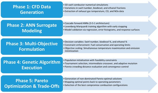
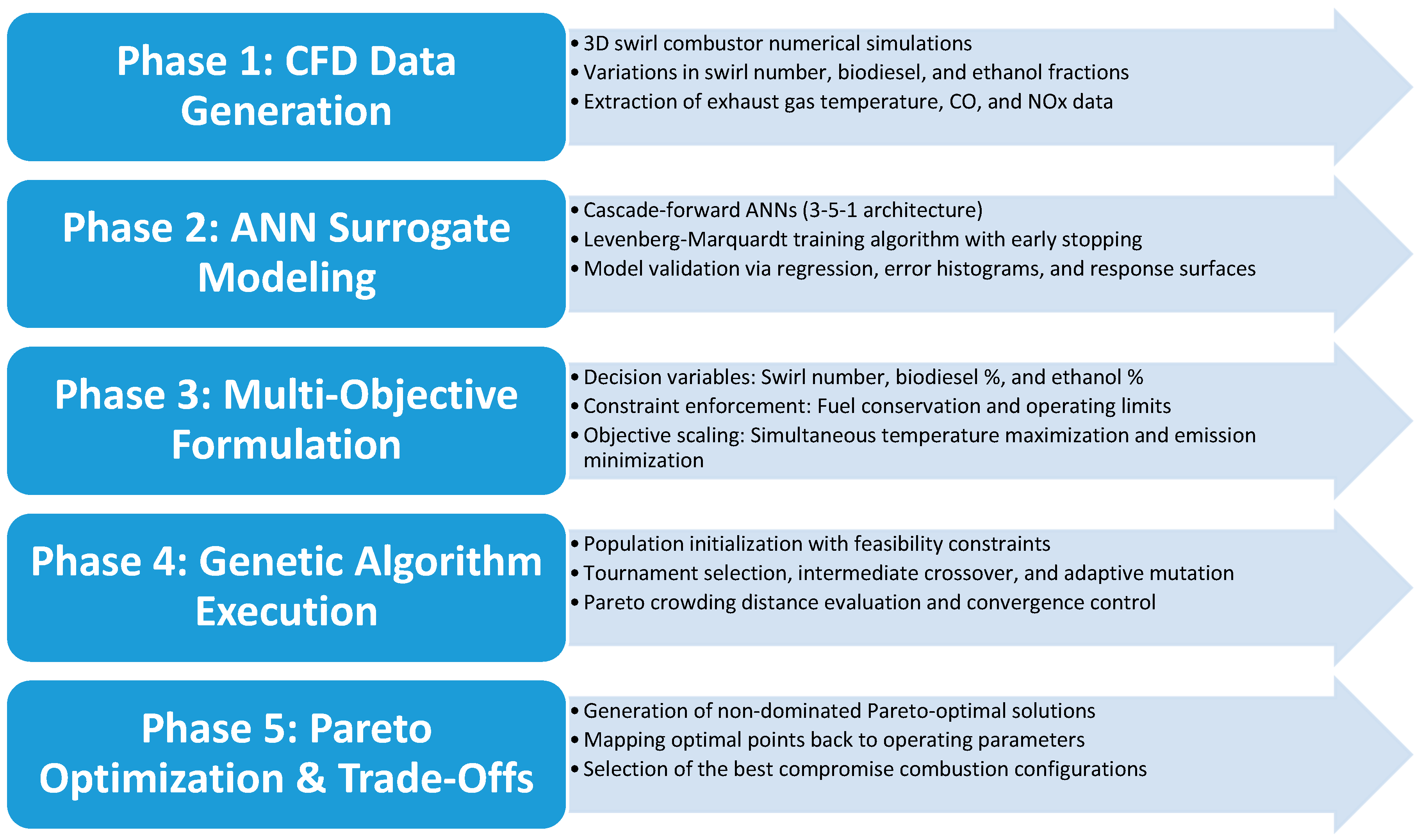
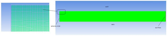
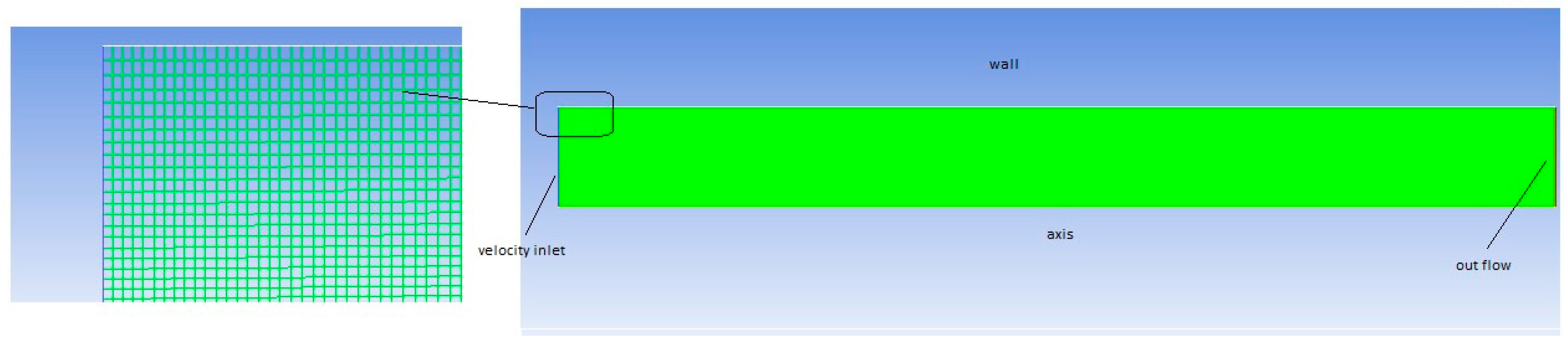
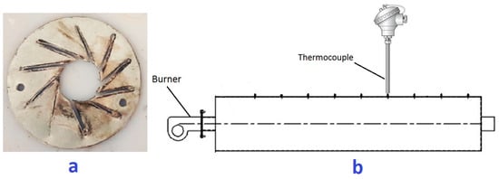
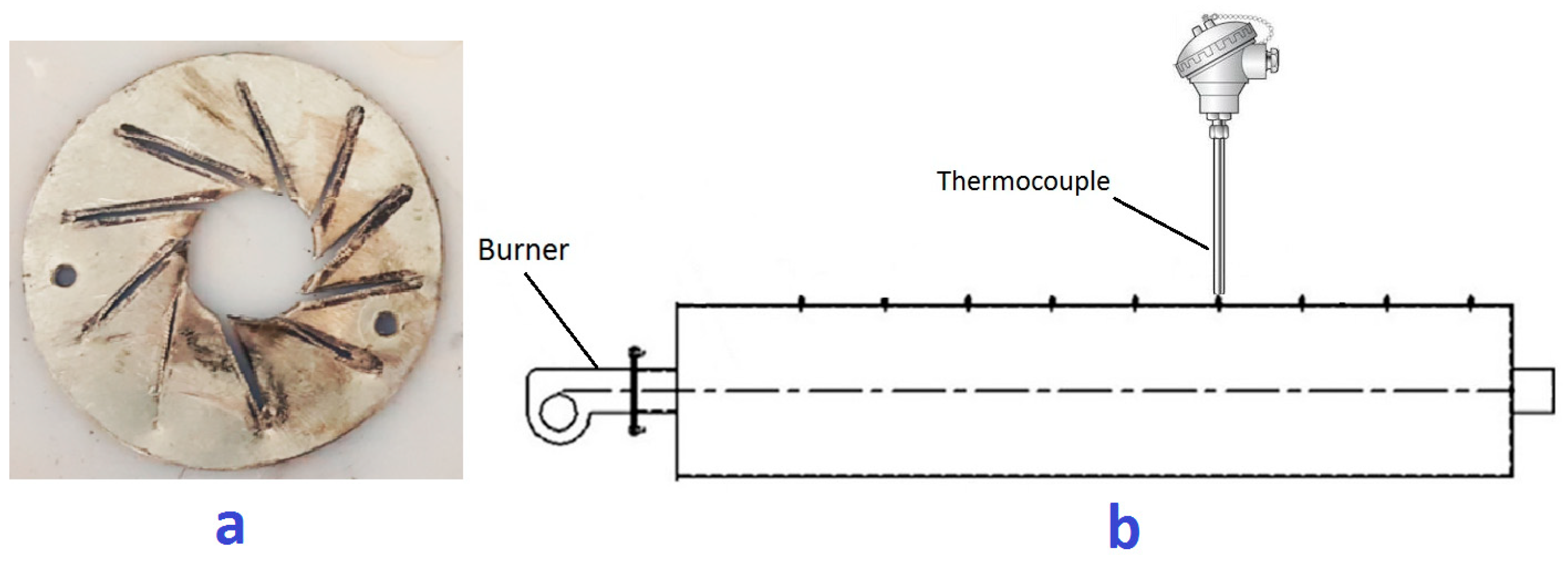
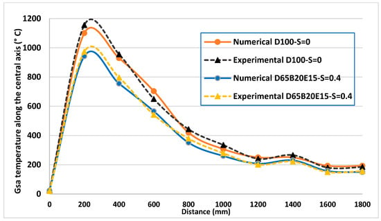
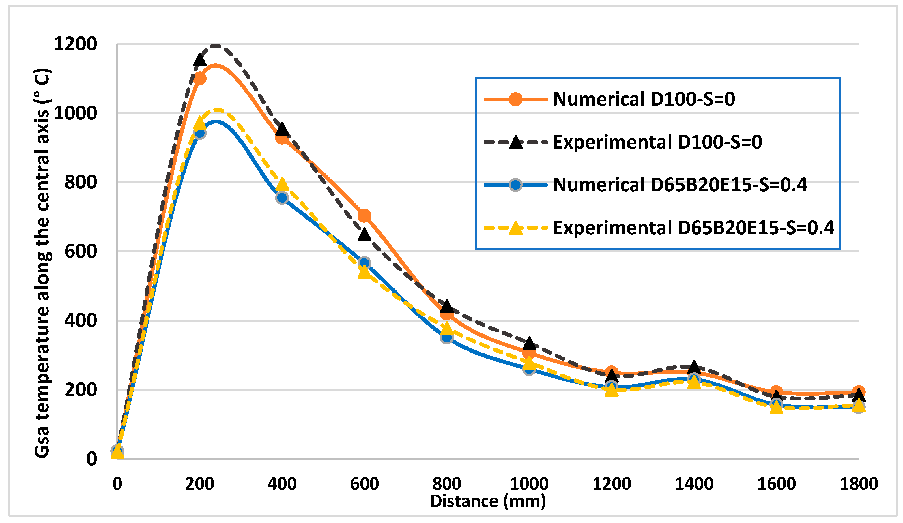
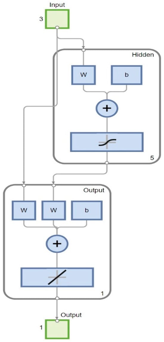
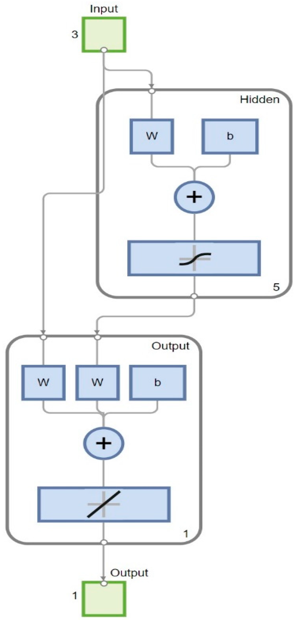
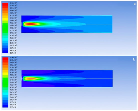
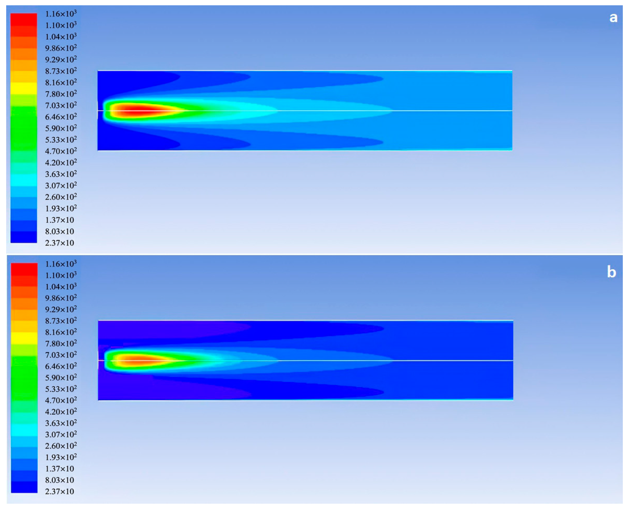
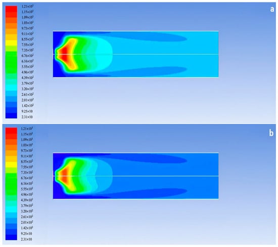
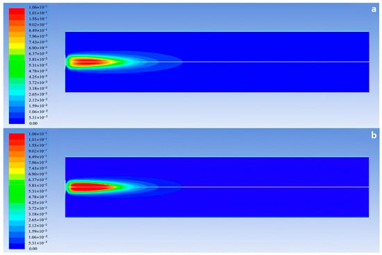
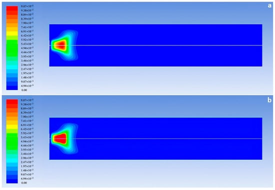
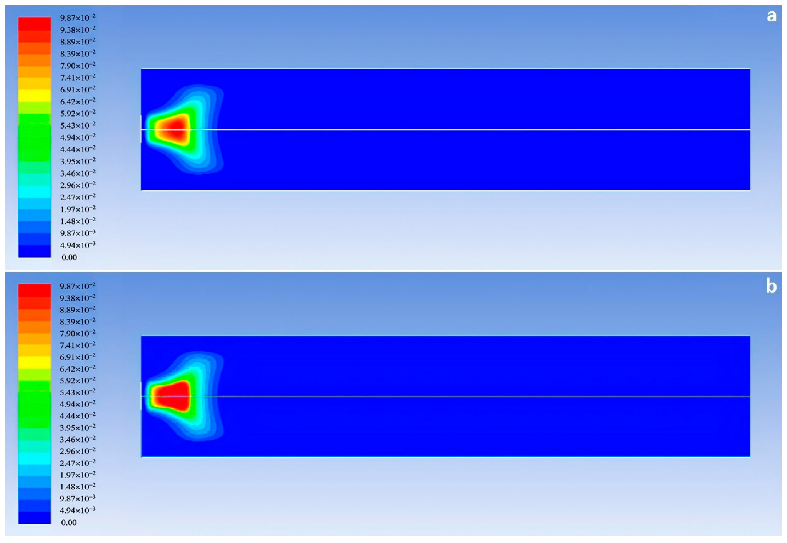
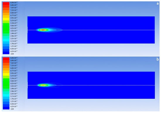
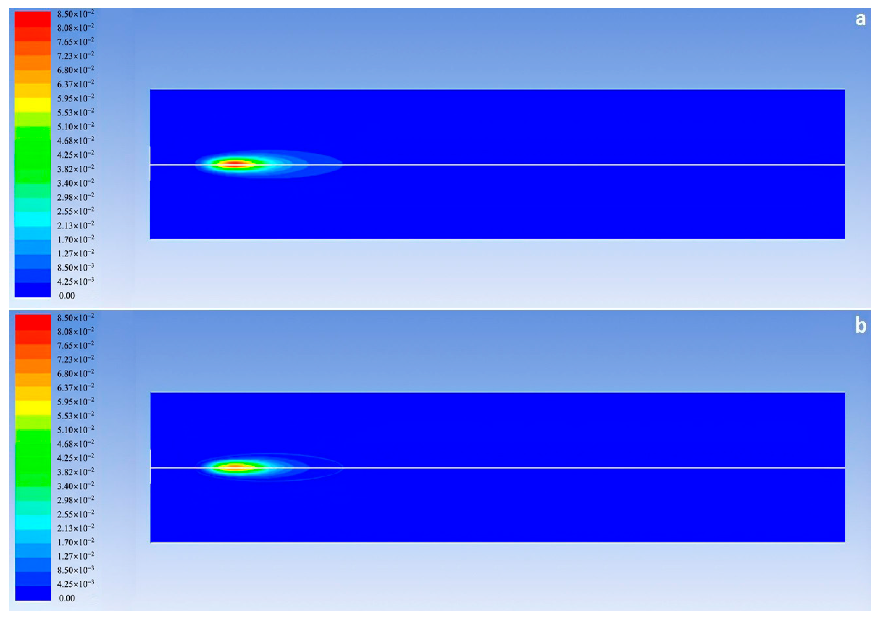
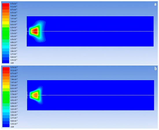
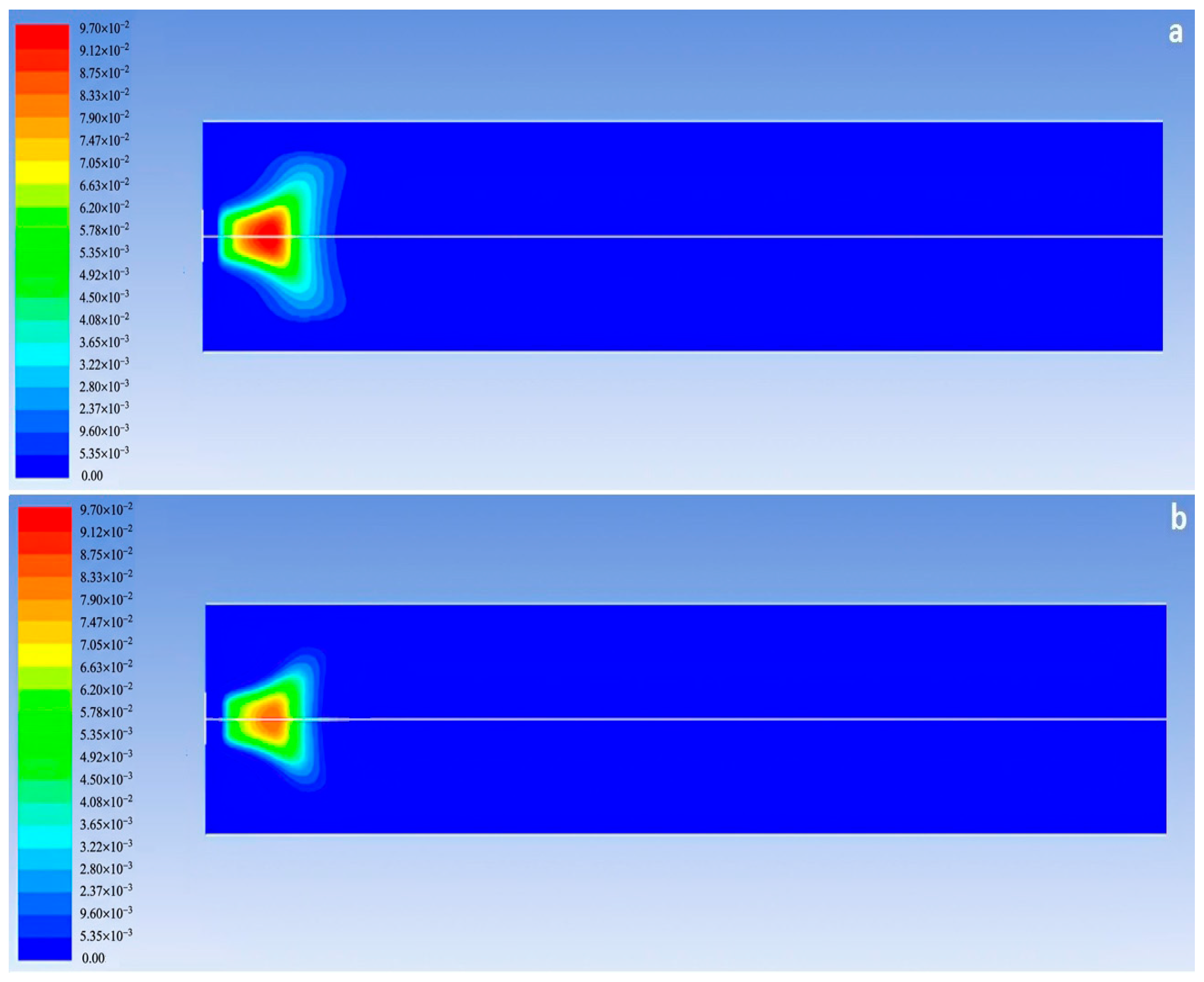
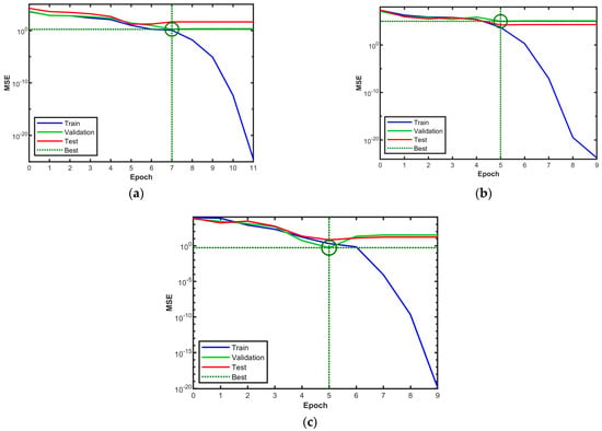
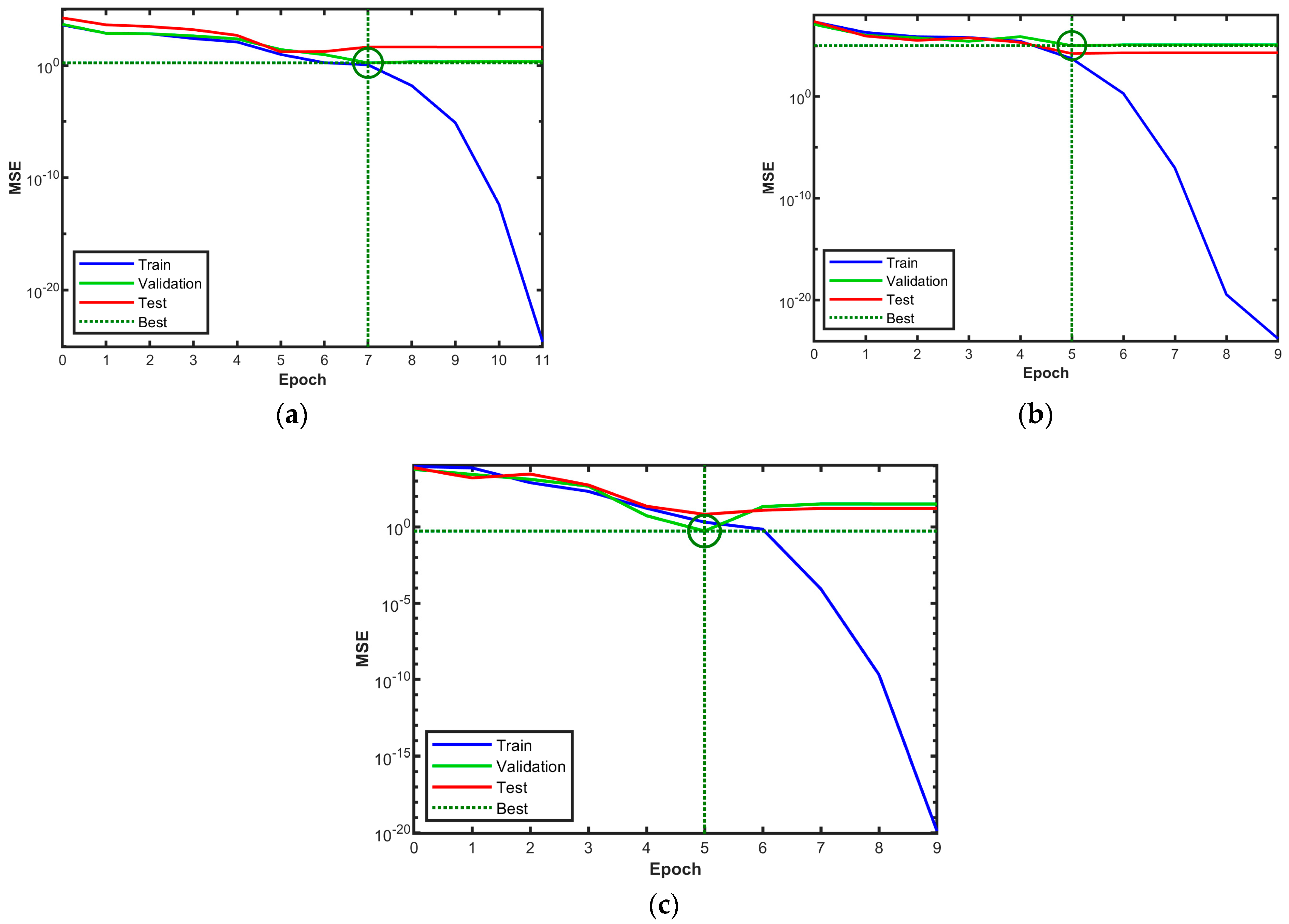
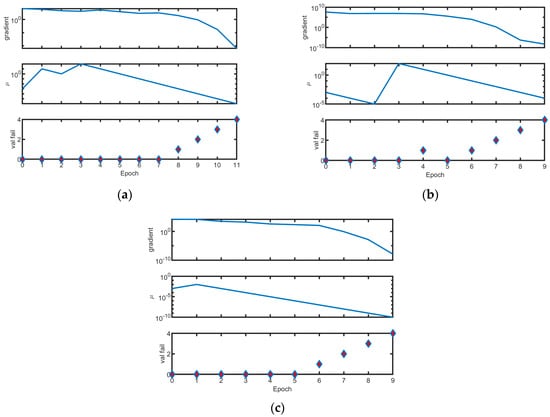
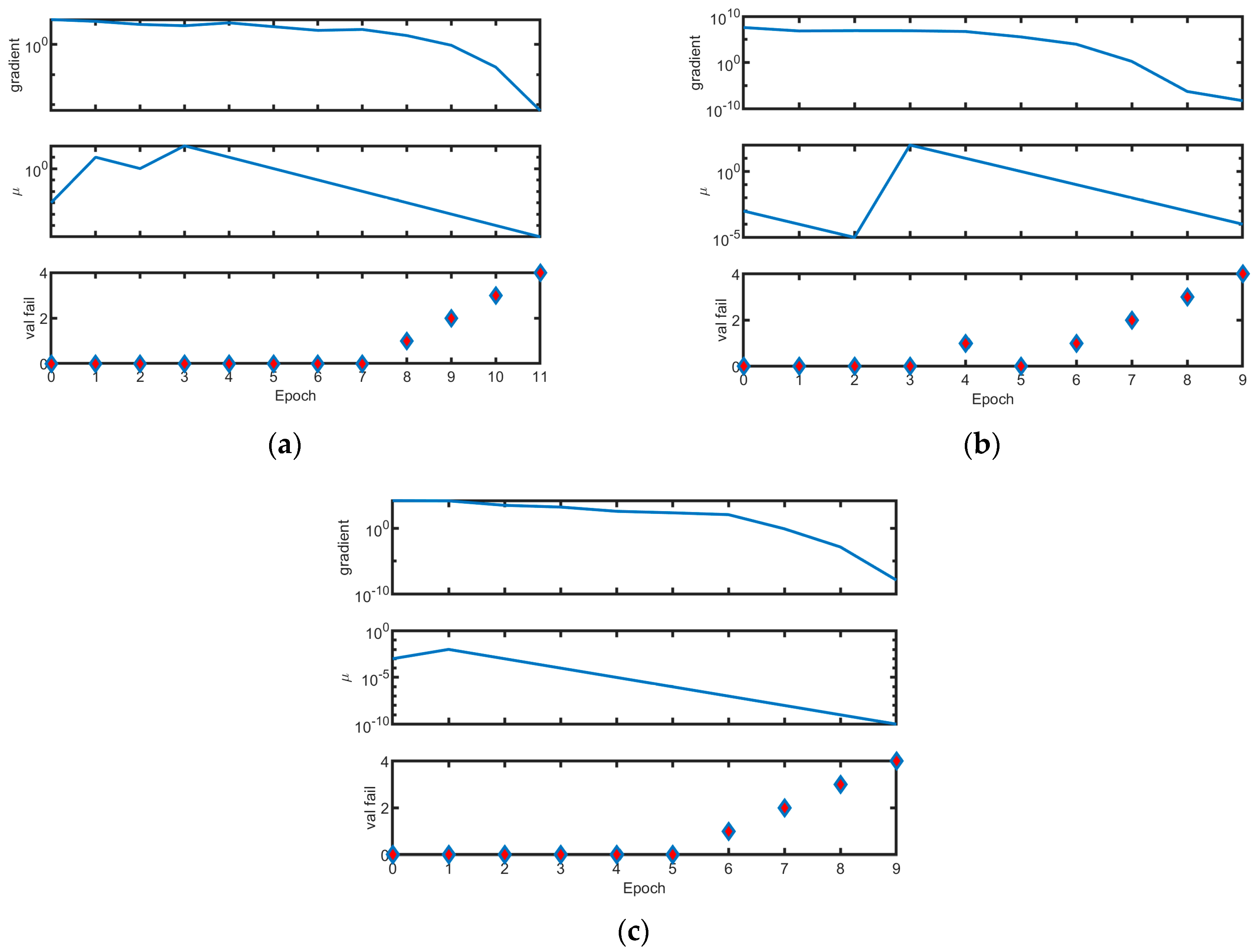
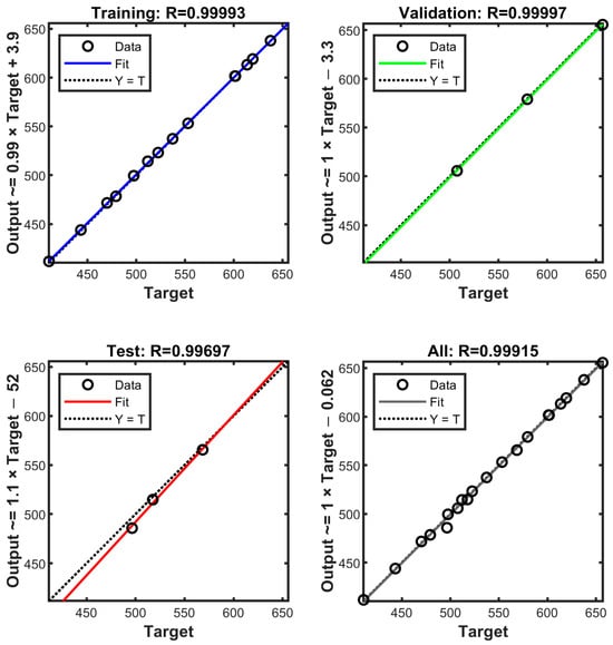
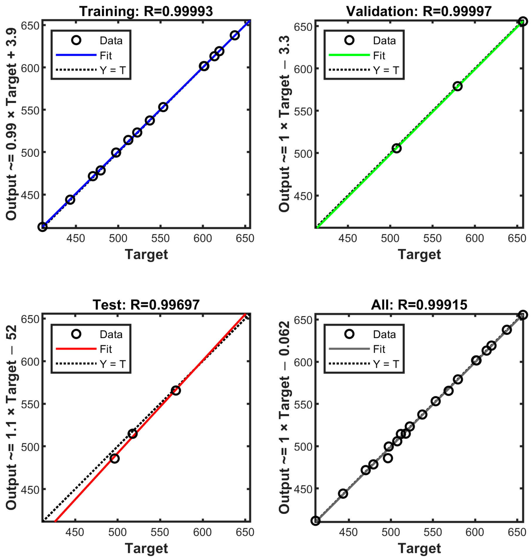
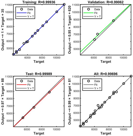
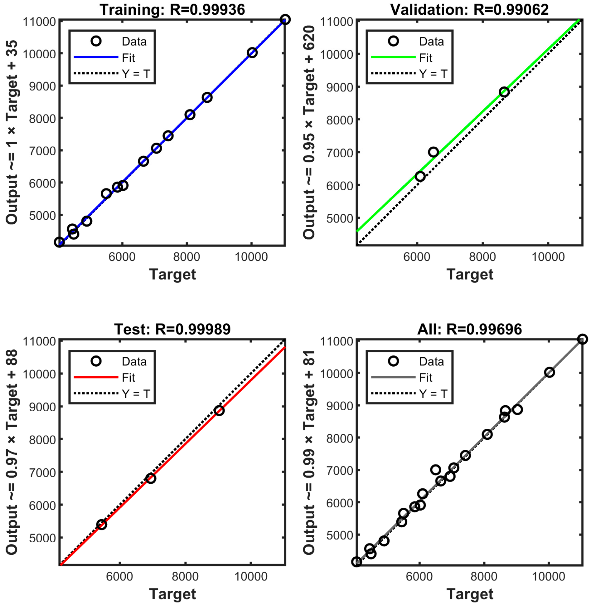
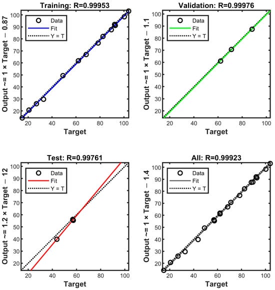
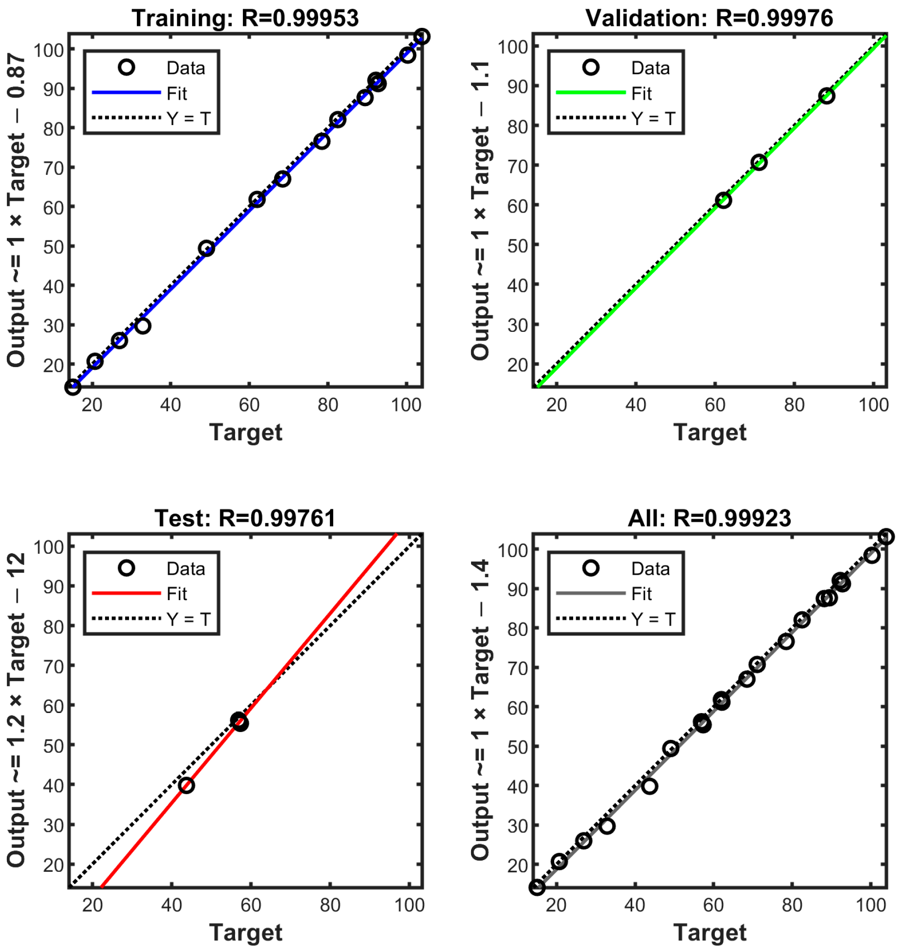
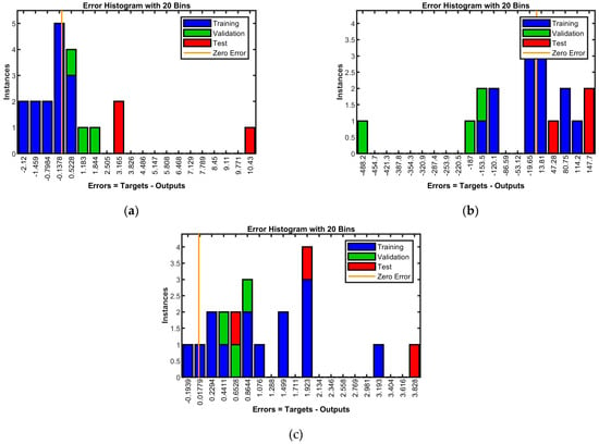
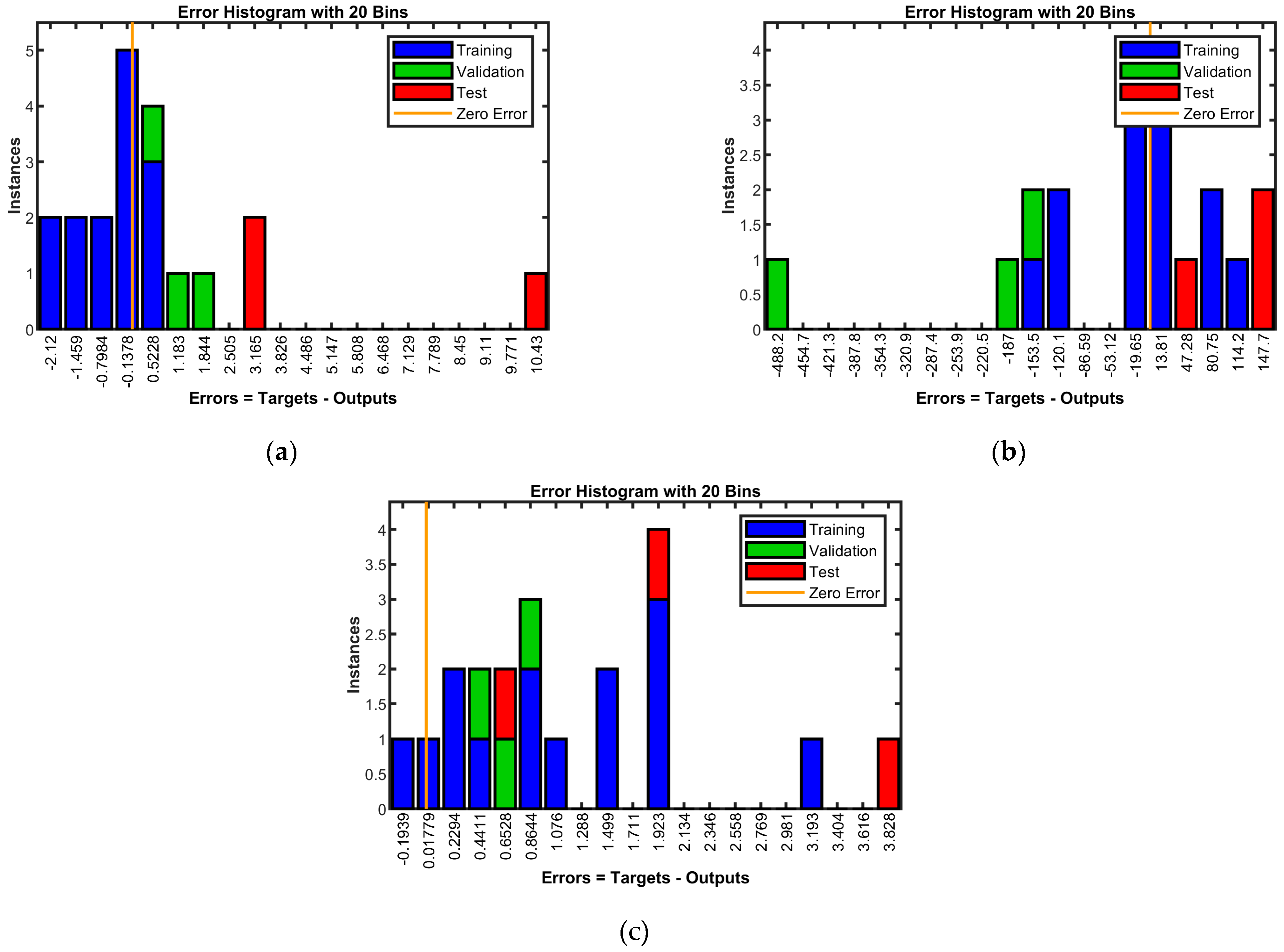
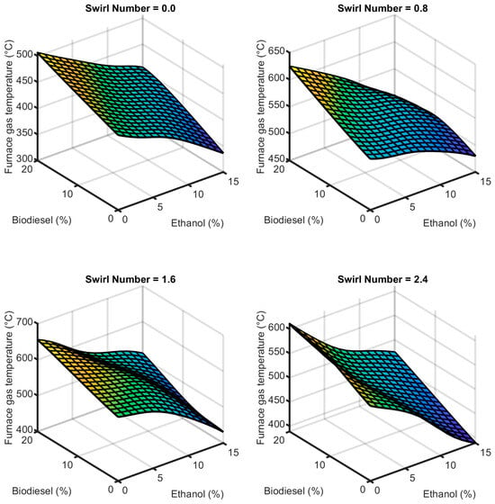
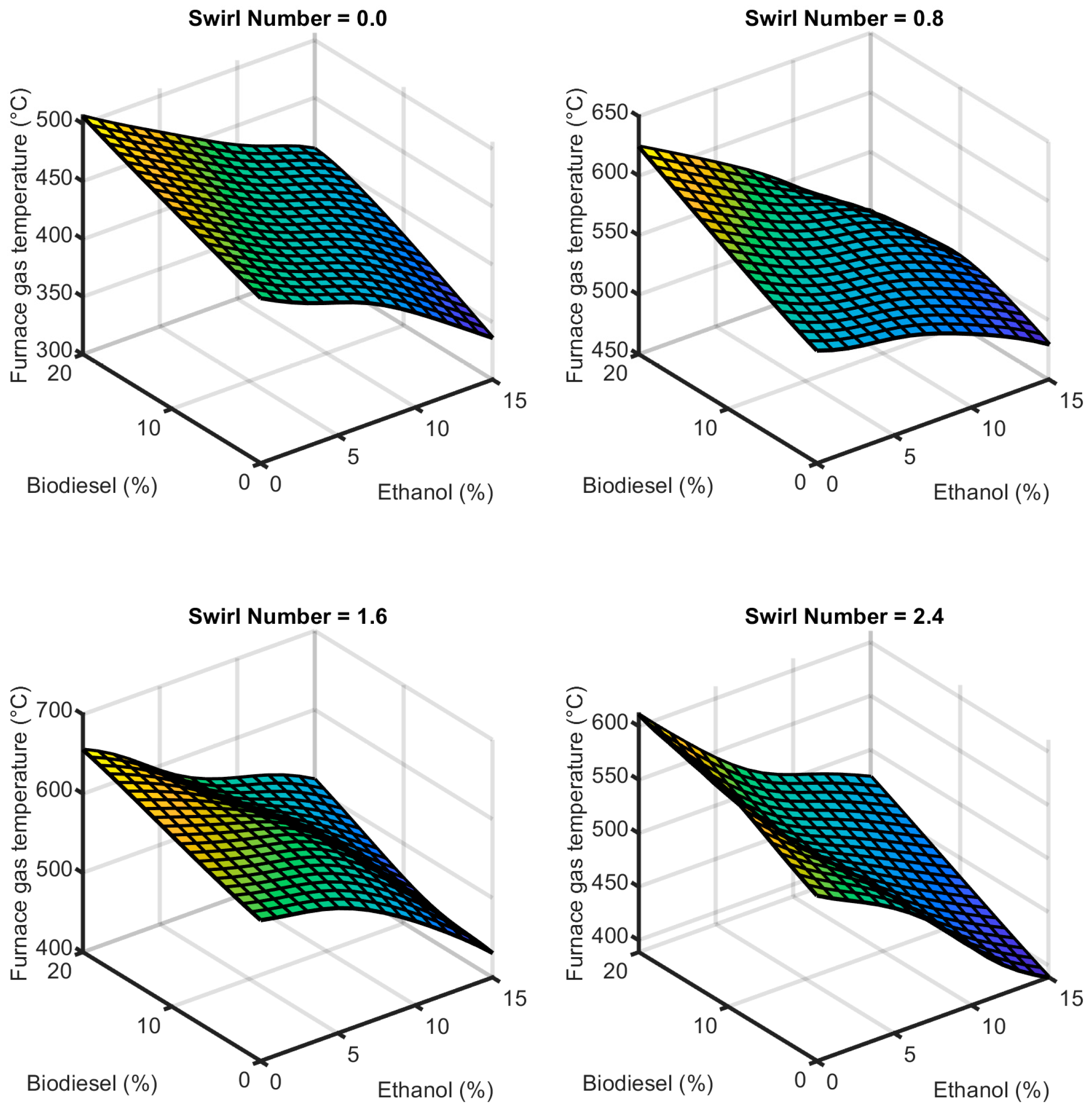
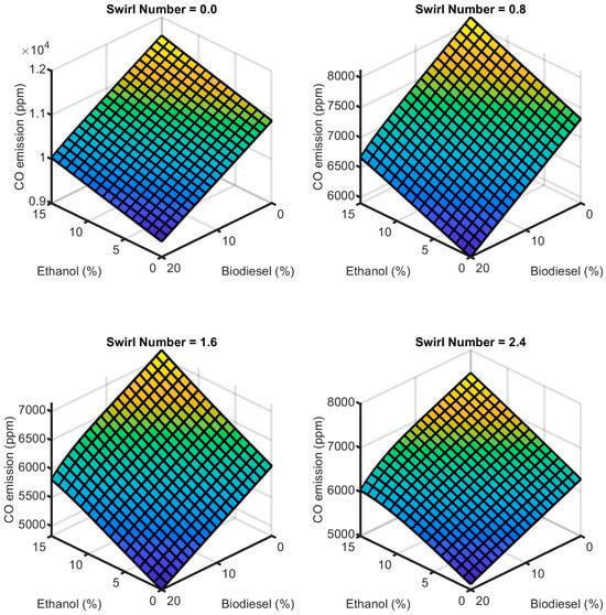
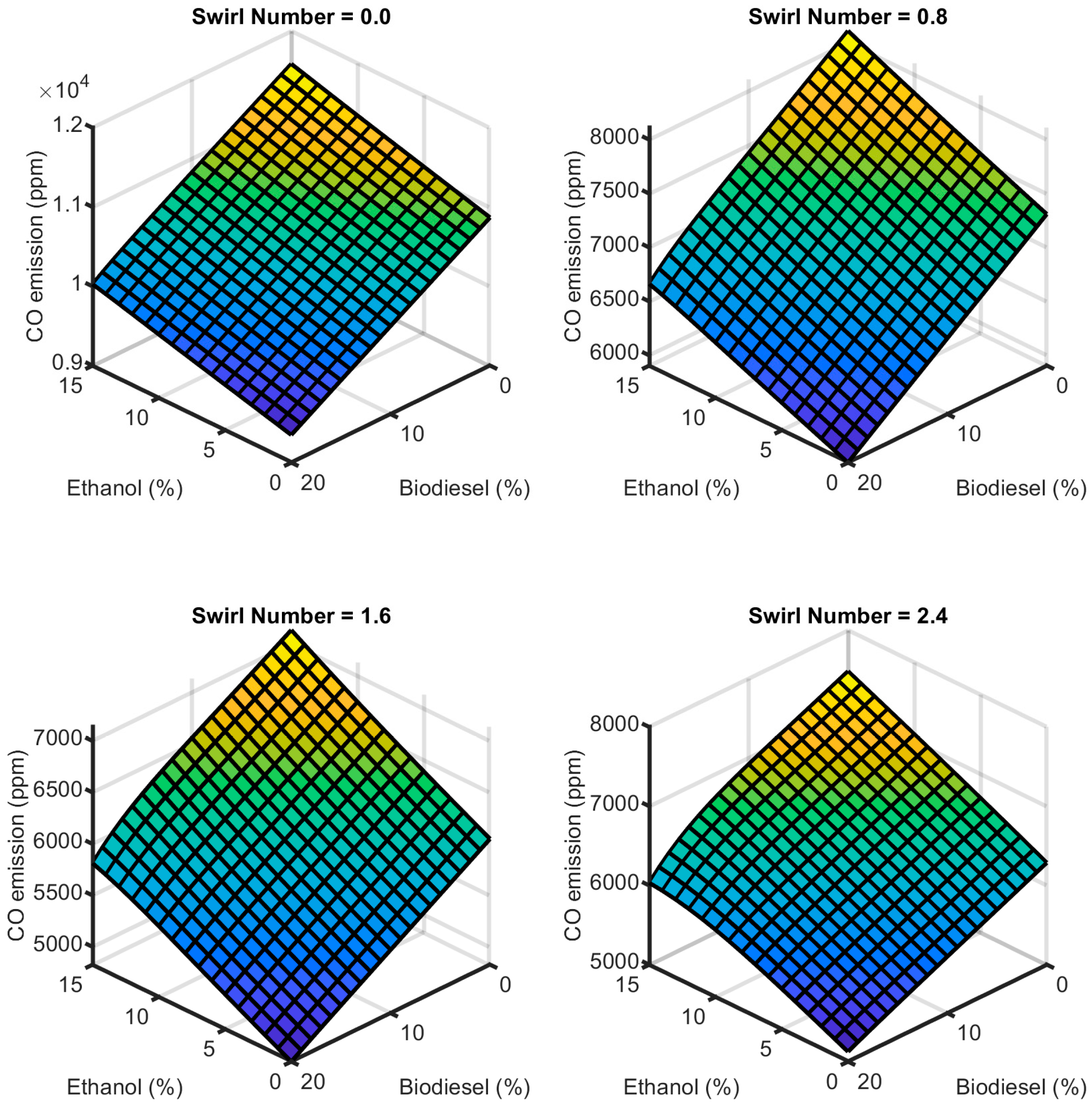
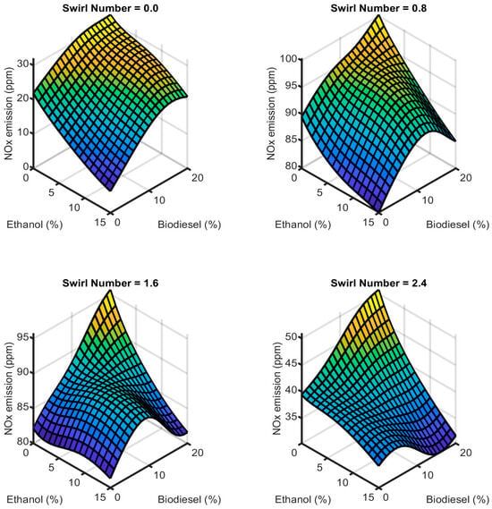
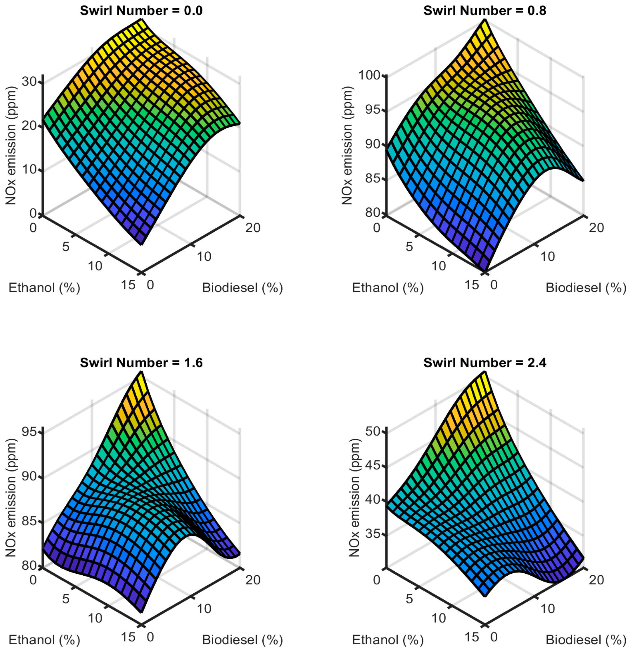
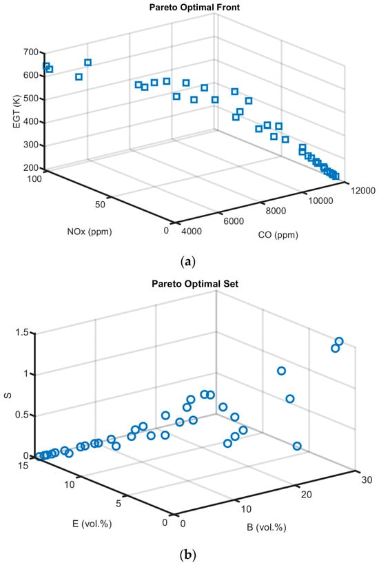
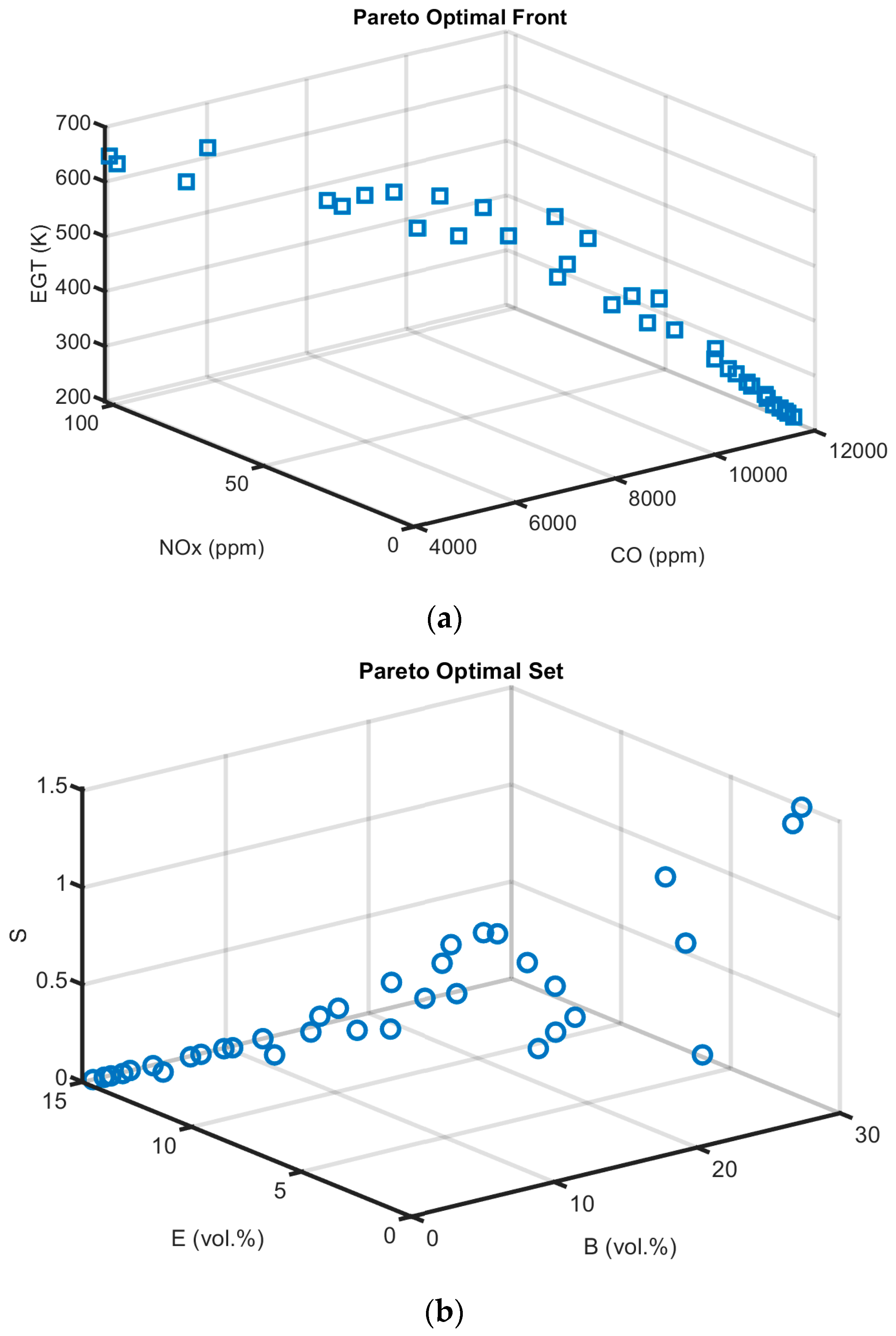

Disclaimer/Publisher’s Note: The statements, opinions and data contained in all publications are solely those of the individual author(s) and contributor(s) and not of MDPI and/or the editor(s). MDPI and/or the editor(s) disclaim responsibility for any injury to people or property resulting from any ideas, methods, instructions or products referred to in the content. |
© 2026 by the authors. Licensee MDPI, Basel, Switzerland. This article is an open access article distributed under the terms and conditions of the Creative Commons Attribution (CC BY) license.