Weighting and Mileage Coding in Grouped Vehicle Emission Regression

Abstract

Weighting rules and mileage coding can change the apparent fit, uncertainty, and predictive performance of regression models built from grouped emission summaries. We examine these choices in a computational case study of 18 supplied age–mileage cells for carbon monoxide, non-methane hydrocarbons, and nitrogen oxides. Age-only, ordinal-mileage, and categorical-mileage specifications are compared using four weighting rules, cell deletion, robust regression, and cross-validation. Categorical mileage represents the lower middle-class means that ordinal coding cannot capture and improves prediction within the supplied grid, including when an entire age level is withheld. However, its advantage is conditional on the mean pattern and can reverse under a correctly specified ordinal model or contamination at the reference cell. Additional simulations with estimated cell dispersions show that interval coverage depends on covariance choice, contamination location, and model specification; small residual-based standard errors do not establish population precision. For practice, weights should reflect a stated estimation target, mileage coding should be checked against the observed shape, and fit should be assessed separately from prediction. The supplied counts sum to 1000, but their measurement lineage and disagreement with assignment frequencies remain unresolved. The findings therefore concern the computational behavior of supplied summaries and constructed scenarios, rather than causal effects or a verified vehicle population.

1. Introduction

Vehicle emission assessment increasingly relies on statistical models to describe how pollutant concentrations and emission rates vary with vehicle characteristics and operating conditions. Vehicle age and accumulated mileage are commonly considered relevant explanatory variables because they may reflect differences in mechanical deterioration, maintenance history, and long-term operating conditions. However, these relationships are difficult to interpret when measurements are available only as grouped summaries rather than individual vehicle observations. Grouped datasets typically report an emission mean, standard deviation (SD), and sample count for each combination of explanatory variables. Although such summaries support regression analysis, they introduce methodological questions concerning observation weights, model specification, uncertainty estimation, and predictive reliability.

A central issue concerns the distinction between within-group dispersion and the precision of a grouped mean. The SD describes variation among measurements within a cell, whereas the sampling variance of its mean also depends on the number of observations and their dependence structure. Consequently, inverse-squared-SD weighting does not necessarily represent inverse sampling variance weighting. Under independent sampling with suitable variance assumptions, count-informed weights provide a more direct approximation to the precision of grouped means. However, their statistical interpretation becomes uncertain when observations involve repeated measurements, unequal sampling probabilities, or unrecognized clustering. Weighted least squares (WLS) inference therefore requires more than selecting a convenient weighting formula. Its reliability also depends on the assumed covariance structure and the relationship between the fitted model and the underlying data-generating process [1].

Model specification introduces another important source of uncertainty. In grouped vehicle emission datasets, mileage is often represented by ordered categories such as low, normal, and high. Assigning these categories numerical values of 1, 2, and 3 simplifies regression estimation but imposes equally spaced effects. When mileage interacts with vehicle age, this representation additionally constrains how age-related emission patterns differ across mileage categories. Such restrictions may be inappropriate when the underlying relationship is nonlinear or nonmonotonic. A categorical representation relaxes these assumptions by estimating separate mileage effects and age interactions. Nevertheless, greater flexibility increases the number of model parameters, making the balance between specification accuracy and estimation stability particularly important when relatively few grouped observations are available [2].

Weighting and model specification should therefore be examined together rather than treated as independent analytical decisions. A weighting rule determines how strongly each observation contributes to estimation, whereas the regression structure determines which relationships the model can represent. Changing observation weights cannot necessarily correct an incorrectly specified conditional mean. Conversely, increasing model flexibility may improve training fit while introducing additional estimation variability. These trade-offs become especially important when researchers compare models using weighted coefficients of determination or residual errors calculated from the same observations used during fitting. Improved training performance does not establish better predictive performance, particularly when model selection and evaluation are not adequately separated [3].

Predictive evaluation provides a complementary perspective on these methodological choices. For grouped emission data, leave-one-cell-out cross-validation offers a way to examine how models predict an omitted age–mileage combination using the remaining grouped observations. Unlike training-fit statistics, this procedure evaluates errors on cells excluded from the corresponding estimation step. However, its interpretation depends on the validation structure. When other observations remain available at the same ages and mileage categories, the exercise primarily assesses prediction within the observed grouping structure. It does not establish transferability to independent fleets, different measurement conditions, or individual vehicles. Consequently, predictive comparisons must be interpreted alongside the sampling design, model complexity, and available measurement metadata [4,5,6].

Uncertainty estimation and robustness assessment provide further information that conventional regression summaries may overlook. Model-based covariance estimates depend on assumptions about residual variance, while heteroskedasticity-consistent estimators offer alternative uncertainty calculations. Cell deletion analysis can identify observations that substantially influence fitted coefficients or reference predictions. Robust regression methods, including Huber estimation, address sensitivity to unusually large residuals, but they do not automatically correct structural misspecification. Similarly, perturbing regression weights can reveal how reference estimates respond to plausible changes in the relative importance assigned to individual cells. These approaches examine different aspects of model dependence and should not be treated as interchangeable evidence of reliability [7].

Controlled simulation experiments can help distinguish these effects under explicitly defined conditions. By varying sample counts, within-cell dispersion, residual contamination, and the functional form of the conditional mean, simulations allow competing estimators to be assessed against known reference values. Such experiments complement empirical comparisons because their assumptions and evaluation targets are specified in advance. They also help distinguish improvements attributable to precision weighting from those associated with robust estimation or more flexible mileage coding. Nevertheless, simulation results remain conditional on the selected scenarios and cannot independently establish the validity of an empirical vehicle emission dataset [8].

This study examines how weighting, mileage coding, and covariance estimation interact when regression is based on a small table of grouped summaries. Established methods provide the estimation and diagnostic tools [1,4,7,8], while recent cross-validation research clarifies why predictive conclusions depend on the evaluation target [9]. The additional value lies in identifying which modeling decisions account for changes in fit, prediction, and uncertainty under a common design. The supplied-data comparisons and controlled simulations show that changing weights cannot compensate for an ordinal specification that excludes a middle-category dip or rise. Conversely, categorical flexibility does not consistently reduce estimation error when the ordinal mean is correctly specified. The covariance comparisons further show that nominal interval coverage can vary substantially even when the fitted mean specification remains unchanged. Together, these results distinguish gains associated with mean specification from those associated with weighting and interval construction. The contribution is a comparative methodological analysis using established estimators, with conclusions restricted to the supplied grouped summaries and specified simulation conditions. The contributions are as follows.

• An auditable case study design separating supplied cell summaries from unverified measurement provenance and distinguishing within-cell dispersion weights from precision weights based on reported counts.
• A comparison of age-only, ordinal-mileage, and categorical-mileage specifications under a common input grid, with separate training-fit, omitted-cell, and omitted-age-level prediction targets.
• A joint assessment of residual-scale, HC3, and unscaled plug-in covariance, together with deletion, Huber fitting, and bounded relative weight sensitivity.
• Controlled simulations examining both known and estimated dispersions, alternative mileage patterns, multiple contamination locations and severities, and the RMSE and interval coverage of the reference estimate.
• A practical interpretation of when weighing, robustness, and functional flexibility help, with explicit limits on population, causal, and external generalization claims.

2. Materials and Computational Methods

2.1. Dataset and Input Verification

The analytical input is a supplied grouped table rather than an independently reconstructed vehicle emission sample. The JRC Euro 7 dataset [10] and related durability report [11] provide background on an external measurement program; their citation does not authenticate the derivation of Table 1. The source manuscript reports 445 JRC tests, whereas the supplied cell counts sum to 1000. No verified mapping establishes whether those counts refer to unique vehicles, repeated tests, expanded records, or constructed frequencies. Accordingly, all subsequent empirical calculations are interpreted as a computational case study of the supplied summaries.

Table 1. Grouped vehicle emission data used in the computational case study. The table presents vehicle age, mileage category, reported cell counts, and pollutant means and standard deviations (SDs). Emission values are expressed in mg/km as supplied.

Cell	Age (Years)	Class	n	CO Mean	CO SD	NMHC Mean	NMHC SD	NOx Mean	NOx SD
g01	0.5	1	53	412.5	48.2	22.4	3.1	8.9	0.95
g02	0.5	2	64	398.7	45.6	21.1	2.9	8.5	0.91
g03	0.5	3	43	425.1	52.4	23.6	3.4	9.6	1.08
g04	1.0	1	50	405.3	46.8	21.8	3.0	8.7	0.93
g05	1.0	2	72	392.4	44.1	20.6	2.8	8.3	0.89
g06	1.0	3	40	418.9	51.2	22.9	3.3	9.3	1.04
g07	2.0	1	58	398.1	45.3	20.9	2.9	8.4	0.90
g08	2.0	2	79	385.6	43.0	19.8	2.7	8.0	0.86
g09	2.0	3	46	411.2	49.7	22.1	3.2	9.0	1.01
g10	3.0	1	52	391.4	44.6	20.4	2.8	8.2	0.88
g11	3.0	2	76	379.3	42.1	19.2	2.6	7.8	0.84
g12	3.0	3	43	404.6	48.9	21.4	3.1	8.8	0.99
g13	4.0	1	55	385.9	43.9	20.0	2.7	8.0	0.87
g14	4.0	2	67	373.7	41.5	18.7	2.5	7.6	0.83
g15	4.0	3	45	398.2	48.1	20.8	3.0	8.6	0.97
g16	5.0	1	52	380.8	43.2	19.6	2.6	7.8	0.85
g17	5.0	2	64	368.4	40.8	18.2	2.4	7.4	0.81
g18	5.0	3	41	392.7	47.4	20.3	3.0	8.4	0.95

Note: Age is expressed in years; mileage classes 1, 2, and 3 represent low, normal, and high mileage, respectively. CO denotes carbon monoxide, NMHC denotes non-methane hydrocarbons, and NOx denotes nitrogen oxides. The reported counts (n) sum to 1000. These counts have not been independently verified as distinct measured vehicles. The derivation of the grouped observations from the Joint Research Centre (JRC) test records, including selection, aggregation, and unit conversion, remains unverified. All numerical values are retained from the supplied analytical dataset.

The analytical inputs were taken from the Summary sheet of the supplied sample count workbook. This sheet contained 18 age–mileage cells with reported counts totaling 1000. These counts were not independently verified as numbers of distinct measured vehicles. The dataset included six vehicle age values (0.5, 1, 2, 3, 4, and 5 years), three mileage categories, and cell-level means and standard deviations (SDs) for carbon monoxide (CO), non-methane hydrocarbons (NMHC), and nitrogen oxides (NOx). All 18 cells had finite means, positive SDs, and positive integer counts ranging from 40 to 79. The grouped cell was the analytical unit, and all cells were retained. The workbook also contained a Samples sheet with 1000 observations generated from normal distributions using the supplied group means and SDs, as documented in its Notes sheet. These generated observations were excluded from regression estimation. All grouped regressions used the summaries reported in Table 1.

Although the grouped dataset was associated with the JRC research source, the available materials did not contain the complete record-level extraction and aggregation procedure connecting the original JRC measurements to the 18 analytical cells. Consequently, the selection criteria, pollutant unit conversions, and construction of the reported sample counts could not be independently reconstructed. The reported regressions were performed using the supplied grouped values rather than recalculated from individual JRC records. This distinction preserves the reproducibility of the statistical calculations without implying that the original measurement provenance has been fully verified.

An additional consistency assessment examined the Samples_Real_Resampled sheet of the supplied 18-cell workbook. Its documentation stated that CO and NOx values were resampled with replacement from the JRC test data and assigned to the 18-cell structure. The sheet contained 1000 rows, with 56 assigned to each of cells g01–g10 and 55 to each of cells g11–g18. These frequencies differed from the counts in Table 1 in 17 cells; g13 was the only matching cell. The resampled rows were excluded from regression estimation because their assigned groups did not establish measured age–mileage relationships. NMHC was absent from the supplied JRC test workbook and the resampled sheet; the NMHC analyses therefore used only the supplied group summaries. All count-informed regressions used the counts in Table 1.

Vehicle ages below one year were represented by 0.5 years, while the remaining age values ranged from one to 5 years. Mileage categories were coded as 1 (low), 2 (normal), and 3 (high). Exact odometer distance boundaries, vehicle composition, the observation period underlying the grouped subset, repeated measurement structure, and emission test conditions could not be fully established from the available analytical files. Documentation published by the United States Environmental Protection Agency (EPA) describes standardized vehicle emission testing procedures [12] but does not independently establish the testing protocol or provenance of these grouped observations. These limitations restrict fleet-level interpretation and external generalization, while the supplied cell summaries remain sufficient to reproduce the reported regression and simulation calculations.

The six age values and three mileage labels were inherited from the supplied table, not chosen through an optimization or a verified sampling protocol. The value 0.5 represents the supplied below-one-year category; an interval definition or midpoint rule for the other age labels is unavailable. We therefore use these numerical ages as modeling inputs without claiming that they are exact individual ages. The six levels provide repeated mileage contrasts across the supplied grid. Classes 1, 2, and 3 describe reported low, normal, and high accumulated mileage, respectively; they are not verified distance intervals or equally spaced odometer values. Their physical cutoffs and possible dependence on vehicle age remain unknown. Ordinal coding is consequently an explicit functional assumption, while categorical coding avoids an equal-spacing assumption without recovering missing physical definitions. The grouped numerical inputs and accompanying workbook documentation are provided in Supplementary Files S1 and S2.

2.2. Regression Specifications and Weighting

Let g index cells and p index pollutants. The outcome is the cell mean $y_{gp}$, with within-cell standard deviation $s_{gp}$, count $n_g$, age $a_g$, and mileage code $m_g$. We fitted the A and AM specifications:

$$y_{gp}={\beta }_{0p}+{\beta }_{ap}{a}_g+e_{gp}$$

(1)

$$y_{gp}={\beta }_{0p}+{\beta }_{ap}{a}_g+{\beta }_{mp}{m}_g+{\beta }_{amp}{a}_g{m}_g+e_{gp}$$

(2)

We fitted a CAT specification by replacing ordinal mileage and its interaction with two category indicators and their age interactions. With mileage 1 as the reference category, its six columns were the intercept, age, the indicators for categories 2 and 3, and the two corresponding age interactions. A and AM contained two and four coefficients, respectively. We used the same 18 cells for every fit within each pollutant [13].

We evaluated reference predictions at age 5 years and mileage category 2. The design vectors were (1, 5) for A, (1, 5, 2, 10) for AM, and (1, 5, 1, 0, 5, 0) for CAT. Each prediction was calculated as the design vector product with the fitted coefficient vector. Differences between specifications measured changes in the fitted reference value rather than causal mileage effects [14].

The reference setting is the observed cell g17 in Table 1, not an independently withheld or external prediction case. It was selected as a common late-age, middle-mileage diagnostic so that all specifications can be compared at identical covariates. Its use does not confer population representativeness or forecast status. Contaminating g17 can directly affect this target, which motivates the additional nonreference contamination scenarios in Section 2.8.

$${\widehat{\beta }}_p={\left(X^{\mathrm{T}}{W}_{p}X\right)}^{-1}{X}^{\mathrm{T}}{W}_p{y}_p$$

(3)

Here, X denotes the design matrix and $W_p$ the diagonal weight matrix. We evaluated equal weights, inverse-SD weights, inverse-dispersion weights (${\displaystyle \frac{1}{s_{gp}^2}}$), and count-informed weights (${\displaystyle \frac{n_g}{s_{gp}^2}}$). A WLS solve based on the square-root-weighted design was used; we checked every full-data and training-fold rank. A common positive rescaling of weights leaves the coefficient estimates unchanged.

Independent observations with common within-cell variance ${\sigma }_{gp}^2$ imply $\mathrm{Var}\left(y_{gp}\right)={\displaystyle \frac{{\sigma }_{gp}^2}{n_g}}$. Replacing ${\sigma }_{gp}^2$ by $s_{gp}^2$ gives the count-informed plug-in criterion. This interpretation requires appropriate cell independence and count definitions; clustering or repeated tests could invalidate it. Inverse-dispersion and count-informed weights coincide up to scale when counts are equal. Neither criterion defines a vehicle population mean without target population composition information [15].

The four criteria differ in the information they use and the target they approximate. Equal weights (w_gp = 1) give each supplied cell equal influence. Inverse-SD weights (w_gp = 1/s_gp) moderately downweight dispersed cells but are not inverse variances of cell means. Inverse-dispersion weights (w_gp = 1/s_gp²) treat within-cell variability as a relative reliability score while ignoring counts. Count-informed weights (w_gp = n_g/s_gp²) approximate inverse variances of independent cell means only if the reported counts and SDs have the required sampling interpretation. Thus, the last criterion is a conditional sensitivity analysis here, rather than a verified precision-weighted population estimate.

2.3. Covariance Calculations and Numerical Targets

For a working grouped-cell model with independent residuals and $\mathrm{Var}\left({\epsilon }_p\mid X\right)={\tau }_p^2{W}_p^{-1}$, the residual-scaled coefficient covariance is

$$V_{\mathrm{model},p}={\widehat{\tau }}_p^2{\left(X^{\mathrm{T}}{W}_{p}X\right)}^{-1},\hspace{1em}\hspace{1em}{\widehat{\tau }}_p^2={\displaystyle \frac{{\mathrm{SSE}}_{w,p}}{G-d}}$$

(4)

Here, the weighted sum of squared errors (SSE) is defined in Equation (6). The coefficient count d includes the intercept. We calculated reference estimate standard errors (SEs) as the square root of $x_{\ast }^{\mathrm{T}}V{x}_{\ast }$ and evaluated the heteroskedasticity-consistent covariance estimator (HC3) as an alternative covariance calculation [16]:

$$V_{\mathrm{HC3},p}=B\left({\displaystyle {\displaystyle \sum }_{g=1}^G}{\displaystyle \frac{w_{gp}^2{e}_{gp}^2}{{\left(1-h_{gp}\right)}^2}}{x}_g{x}_g^{\mathrm{T}}\right)B,\hspace{1em}\hspace{1em}B={\left(X^{\mathrm{T}}{W}_{p}X\right)}^{-1}$$

(5)

Here, e is a cell residual, and h is weighted leverage. We used HC3 to evaluate sensitivity to grouped residual heterogeneity. For count-informed fits, we also calculated the unscaled plug-in covariance ${\left(X^{\mathrm{T}}WX\right)}^{-1}$ and retained the corresponding SEs in the companion results. This calculation assumes that the plug-in mean variances are adequate without an estimated common residual multiplier. We reported residual-scaled and HC3 SEs separately. Their numerical evaluation does not establish confidence interval coverage or verify the underlying sampling design [17].

Throughout Equations (1)–(9), $g=1,\dots ,G$ indexes cells ($G=18$), $p$ indexes pollutants, $a_g$ is age, $m_g$ is the ordinal class label, $y_{gp}$ is a supplied cell mean, $s_{gp}$ is its reported within-cell SD, and $n_g$ is its reported count. The vector $x_g$ contains a model’s $d$ regressors, $X$ stacks their transposes, ${\beta }_p$ denotes coefficients, and $e_{gp}=y_{gp}-x_g^{\top }{\widehat{\beta }}_p$ denotes a fitted residual. $W_p$ has diagonal entries $w_{gp}$; $B={\left(X^{\top }{W}_{p}X\right)}^{-1}$; $h_{gp}=w_{gp}{x}_g^{\top }B{x}_g$; ${\tau }_p^2$ is the common residual multiplier in the working model. A hat denotes an estimate, and $x_{\ast }$ denotes the reference design vector at $g_{17}$. The simulation uses ${\mu }_g$ and ${\sigma }_g$ for constructed true means and within-cell SDs, $Z_g$ for a standardized random error, and $R$ for the number of repetitions. These meanings are distinct from observed grouped residuals and the simulation reference error. HC3 inflates contributions from high-leverage residuals through ${\left(1-h_{gp}\right)}^{-2}$. It measures sensitivity to residual heterogeneity but does not reconstruct missing dependence, validate counts, remove misspecification, or guarantee reliable coverage with 18 cells.

We verified the residual-scaled covariance implementation against an independent implementation of the WLS coefficient and covariance calculations. The two implementations agree on the complete grouped table. Additional numerical checks confirmed coefficient invariance to a common weight multiplier, the weighted leverage trace identity, and agreement between direct deletion residuals and the prediction residual sum of squares (PRESS) identity [18].

2.4. Weighted Fit and Cell Prediction

Weighted fit uses the following explicit definitions:

$${\mathrm{SSE}}_{w,p}={\displaystyle {\displaystyle \sum }_{g=1}^G}{w}_{gp}{\left(y_{gp}-{\widehat{y}}_{gp}\right)}^2$$

(6)

$${\overline{y}}_{w,p}={\displaystyle \frac{{\sum }_{g=1}^G{w}_{gp}{y}_{gp}}{{\sum }_{g=1}^G{w}_{gp}}}$$

(7)

$${\mathrm{SST}}_{w,p}={\displaystyle {\displaystyle \sum }_{g=1}^G}{w}_{gp}{\left(y_{gp}-{\overline{y}}_{w,p}\right)}^2$$

(8)

$$R_{w,p}^2=1-{\displaystyle \frac{{\mathrm{SSE}}_{w,p}}{{\mathrm{SST}}_{w,p}}},\hspace{1em}\hspace{1em}{R}_{w,p,\mathrm{adj}}^2=1-\left(1-R_{w,p}^2\right){\displaystyle \frac{G-1}{G-d}}$$

(9)

The weighted total sum of squares (SST) must be positive. We used weighted $R^2$ and adjusted $R^2$ to describe training fit within each weighting criterion. To compare predictions across weight rules, we calculated equal-cell LOCO MSE in the original pollutant units squared [19]. In each fold, we fitted the model on 17 cells and predicted the omitted cell. We retained its prediction, leverage, and change in the reference estimate. This evaluation targeted prediction within the observed grouping structure [9]. Because the same LOCO comparisons informed the assessment of mileage coding, they provided exploratory model comparison rather than independent post-selection validation.

LOCO is useful because every cell is predicted once without being used in its own coefficient fit, and the same equal-cell loss permits comparison across weight rules. Its limitations are overlapping training sets, only 18 prediction errors, retention of other cells at the omitted age and mileage levels, and reuse for exploratory model comparison. It therefore assesses prediction of supplied grouped means rather than prediction of an individual vehicle or transfer to a new fleet. Section 2.8 adds a stricter six-fold age-blocked validation; neither exercise is independent external validation.

2.5. Robust Fitting and Bounded Weight Sensitivity

We fitted Huber regression to evaluate residual sensitivity [20]. The implemented objective was the weighted Huber loss of residuals divided by a fixed training scale, with cutoff 1.345. We initialized the scale as 1.4826 times the median absolute deviation of the inverse-dispersion WLS residuals from their median. Reference weights multiplied the loss outside the residual argument. We solved the objective by iteratively reweighing least squares using $\min \left(1,{\displaystyle \frac{1.345}{\left|u\right|}}\right)$, without an added ridge penalty. We recomputed the scale within each LOCO training set and held it fixed during coefficient optimization. The implementation recorded a failed fit for a nonpositive scale or failure to converge. We independently verified the full-data Huber objectives by direct numerical minimization.

The cutoff 1.345 is the conventional Huber choice yielding approximately 95% asymptotic efficiency for Gaussian location errors with a correctly specified scale [20]. This provides a transparent benchmark rather than an emission-specific optimum. It does not guarantee 95% efficiency for this weighted, small, grouped design, and a robust residual loss cannot repair an ordinal mean structure that excludes a middle-class dip.

We evaluated weight sensitivity for the AM reference prediction. Define normalized reference weights $q_{gp}^0={\displaystyle \frac{w_{gp}}{{\sum }_h{w}_{hp}}}$, with inverse-dispersion w. Feasible weights sum to one and satisfy $q_{gp}^0\exp \left(-\rho \right)\le q_g\le q_{gp}^0\exp \left(\rho \right)$, for $\rho$ = 0, 0.25, 0.5, and 1. At each positive tolerance, sequential least squares programming (SLSQP) minimized and maximized the prediction from eight feasible starting points: the baseline plus seven starts formed by mixing 95% of a linear-programming vertex with 5% baseline weight. Starts used fixed-seed random linear objectives. The solver used analytic prediction derivatives, at most 1000 iterations, and objective tolerance ${10}^{-10}$; feasibility tolerance is ${10}^{-7}$. We included the baseline among attained values. The calculated ranges summarize successful feasible solutions and are approximate attained ranges, not certified global bounds or confidence intervals. Failure statuses are retained in the execution record [21].

The sensitivity implementation enforced the weight bounds and simplex constraint simultaneously, allowing relative cell contributions to change. We checked feasibility, convergence, and the inclusion of the reference solution for every tolerance. The implemented computational scope comprised WLS, covariance comparisons, Huber estimation, cell deletion, LOCO prediction, and bounded weight perturbations. Distributionally robust optimization (DRO) and partial pooling were outside this computational scope [22].

The tolerance ρ is a logarithmic bound on each normalized relative weight: exp(−ρ) ≤ q_g/q_gp⁰ ≤ exp(ρ), together with the simplex constraint. Thus ρ = 0.25, 0.5, and 1 allow individual ratios of approximately 0.779–1.284, 0.607–1.649, and 0.368–2.718, respectively. These are analyst-defined stress levels, not estimated probabilities, count error percentages, confidence levels, or empirically calibrated uncertainty sets. Because weights must still sum to one, their individual extremes cannot generally be attained simultaneously.

2.6. Controlled Simulation Experiments

The simulation used the same fixed age–mileage grid, with no emission measurements. For each scenario and repetition, independent Gaussian grouped means were generated as $y_g={\mu }_g+{\displaystyle \frac{{\sigma }_g{Z}_g}{\sqrt{n_g}}}$. The base mean is 2 + 0.3 × age + 0.2 × mileage + 0.05 × age × mileage, so the target at age 5 and category 2 is 4.4 simulation units. Equal-count scenarios used n = 50; equal-dispersion scenarios used $\sigma$ = 2. Unequal counts, in cell order g01–g18, are (20, 80, 30, 25, 100, 20, 40, 90, 25, 30, 80, 20, 40, 100, 30, 20, 80, 25). Unequal dispersions increased linearly from 1 to 4 over those 18 cells. These are constructed simulation settings, not recovered vehicle counts or variances.

We executed six simulation scenarios: equal counts and SD, unequal counts only, unequal SD only, both unequal counts and SD, contamination, and categorical misspecification. In the contamination scenario, we added six grouped-mean SDs to g17 after generation and evaluated predictions against the uncontaminated target. For misspecification, we added 1.5 to the category 2 mean, changing the reference target to 5.9. These two scenarios otherwise used the combined unequal-count and unequal-SD settings. We ran 1000 repetitions per scenario and fitted five methods in each repetition: equal weight AM, inverse-dispersion AM, oracle count-informed AM, inverse-dispersion CAT, and inverse-dispersion Huber AM. The estimators had access to the known simulation counts and variances. These experiments did not include sample-SD estimation or uncertainty about the sampling design.

We calculated reference prediction bias, RMSE, Monte Carlo SEs, and the number of failed fits. The estimated RMSE Monte Carlo SE is ${\displaystyle \frac{\mathrm{SD}\left(e^2\right)}{2\mathrm{RMSE}\sqrt{R}}}$, where e is the reference error, and R is the number of successful repetitions. We constructed approximately 95% Monte Carlo intervals using 1.96 times this standard error. These intervals quantify simulation error, not vehicle emission uncertainty. We used random seed 20261017 and a single recorded generator for sensitivity starts followed by simulation. Results from the supplied grouped table and executed simulation results were analyzed and presented separately.

The original six scenarios isolate benchmark mechanisms: equal information checks agreement of weighting conventions; unequal counts and unequal dispersions separate their contributions; their combination tests the precision weighting argument; contamination examines residual sensitivity; and the category 2 shift tests an excluded mean pattern. They are diagnostic constructions rather than calibrated vehicle populations. With R = 1000, the binomial Monte Carlo SE coverage near 95% is about 0.0069 (0.69 percentage points), and its maximum over all coverage probabilities is about 0.0158. This repetition count supports comparison of large differences while leaving close rankings uncertain; RMSE Monte Carlo SEs are reported separately. It is not a guarantee of convergence or statistical power for every contrast.

2.7. Computational Implementation and Reproducibility

We implemented the analysis in Python 3.12.14 and assembled the computational inputs, estimation and verification code, figure-generation scripts, coefficients, cell diagnostics, sensitivity solver records, and simulation outputs in a reproducibility archive. The accompanying repository is https://github.com/themanoftalent/MCA_Reproducibility (accessed on 15 October 2026). Input file hashes, software versions, random seeds, and execution logs document the computational workflow and support reproducibility [23,24]. Verification records connect the inputs, analytical procedures, and generated outputs [25]. The archive specifies the Python, NumPy 2.3.5, SciPy 1.17.0, openpyxl 3.1.5, and Matplotlib 3.10.8 versions used. Comparisons with the manuscript tables distinguish reproduced values from newly executed simulation results. Generated and resampled observations are documented separately from measured test records. These materials support verification of the computations; they do not establish the measurement provenance of the supplied grouped summaries.

2.8. Additional Validation and Simulation Analyses

We used the numerical inputs reported in Table 1 for the additional analyses. Leave-one-age-level-out validation comprised six folds. In each fold, all three mileage cells at one age were withheld, each model was fitted to the remaining 15 cells using inverse-dispersion weights, and the three omitted means were predicted. MSE assigned equal weight to all 18 held-out squared errors. The two endpoint folds required extrapolation beyond the retained training ages, whereas the interior folds involved interpolation between retained ages. All training designs had full column rank. We also fitted count-informed A, AM, and CAT models and compared residual-scaled, HC3, and unscaled plug-in standard errors for the same reference estimate. Fitted CAT curves described the pattern within the observed grid without implying mechanistic age effects.

The additional simulations used the base mean, unequal counts, and unequal dispersions specified in Section 2.6, with 1000 repetitions per scenario and a separate NumPy default_rng seed of 20261030. Eleven scenarios covered the base ordinal mean; a monotone category modification adding 0.4 to class 2 and 1.5 to class 3; class 2 shifts of −1.5 and +1.5; contamination at each of $g_{01}$, $g_{09}$, and $g_{17}$ by +3 or +6 true grouped-mean SDs; and the base ordinal mean with standardized $t$-distributed errors with five degrees of freedom. These $t$-distributed errors were multiplied by $\sqrt{3/5}$ to obtain unit variance. The target was the uncontaminated mean at $g_{17}$ under the applicable mean pattern. Contamination was added after sampling, leaving the generated means at other cells unchanged. The selected locations represented a young class 1 cell, an interior class 3 cell, and the reference cell.

In each repetition, independent variance estimates were generated by multiplying the true within-cell variance by an independent chi-square draw with $n_g-1$ degrees of freedom and dividing by $n_g-1$. The variance draws were independent of the generated means. This construction reproduces the sampling relationship between means and variances under independent Gaussian within-cell observations. In the scenario with $t$-distributed mean errors, it served as a dispersion uncertainty stress test. Count-informed AM and CAT models were fitted to the same generated means using either known or estimated within-cell variances.

We recorded the RMSE of the estimated mean at g17, its Monte Carlo standard error as defined in Section 2.6, and coverage of nominal 95% intervals. Plug-in intervals used a normal critical value of 1.959964, whereas residual-scaled and HC3 intervals used t critical values with G − d degrees of freedom. These conventions defined the interval comparisons without guaranteeing finite-sample coverage. Coverage concerned the underlying mean at g17 rather than a future noisy measurement. All 44,000 additional fits produced finite results. The estimated- and known-dispersion results are presented in Section 3.7. The simulations reported in Tables 10 and 11 evaluated AM and CAT interval coverage under independent cell errors. Dependence between cells was examined separately in the sensitivity analyses presented in Section 3.9.

To examine whether the categorical-model advantage depended on additional coefficients, we fitted an additive categorical model (ACAT) containing an intercept, vehicle age, and indicators for mileage categories 2 and 3, with a common age slope across categories. ACAT and AM each contained four coefficients, whereas CAT contained six. We compared these specifications under all four weighting rules using adjusted R², equal-cell LOCO MSE, and leave-one-age-level-out MSE. We also calculated residual-scaled and HC3 standard errors for the coefficients and reference estimate, together with changes in the reference estimate after cell and age-level deletion. These analyses assessed model complexity, uncertainty, and stability within the supplied grouping grid. The validation results supported exploratory model comparisons rather than independent evaluation after model selection.

We conducted six further sensitivity scenarios using the base ordinal mean, unequal counts, and unequal dispersions from Section 2.6. These comprised independent errors; correlations of 0.3 and 0.6 between cells within the same mileage category; count input perturbations with coefficients of variation of 0.25 and 0.50; and correlation of 0.3 combined with count perturbation of 0.50. Correlated standardized errors combined independent cell-specific and shared mileage-category Gaussian components, scaled by the square roots of one minus the specified correlation and the specified correlation, respectively. This preserved the marginal grouped-mean variances and independence between mileage categories. Reported counts were generated by multiplying the true simulation counts by independent lognormal factors with mean one, rounding to the nearest integer, and imposing a minimum of two. The stated coefficients of variation describe the factors before rounding. True counts governed data generation, while perturbed counts entered the estimation weights.

Each scenario used 1000 repetitions with random seed 20261031. Count-informed AM, ACAT, and CAT models used independently generated chi-square variance estimates as described above. The same underlying random draws were reused across scenarios, and all models within a scenario received identical inputs. We recorded bias, empirical standard deviation, RMSE, Monte Carlo standard errors, and interval coverage for the estimated mean at g17. All interval calculations retained the diagonal covariance assumptions and critical value conventions used in the preceding simulations. The dependence and count perturbation levels were specified sensitivity settings rather than estimates from Table 1. All 18,000 fits produced finite results.

3. Results

3.1. Reference Estimates and Implementation Verification

The computational pipeline fitted all three specifications for each pollutant and reproduced the coefficient and covariance calculations in the independent verification. Under inverse-dispersion AM, the reference estimates were 378.537 mg/km for CO, 19.096 mg/km for NMHC, and 7.790 mg/km for NOx. Weighted R² was 0.6083, 0.6098, and 0.6146, respectively. Table 2 presents the complete reference prediction, covariance, training-fit, and LOCO results for the inverse-dispersion models. All values were calculated from Table 1.

Table 2. Calculated inverse-dispersion regression results for the supplied grouped table. Working SE uses residual scaling; HC3 SE uses the alternative covariance calculation. Estimates and SEs are in mg/km; LOCO MSE is in (mg/km)².

Pollutant	Model	Reference	Working SE	HC3 SE	Weighted R2	LOCO MSE
CO	A	378.222	4.551	4.968	0.5164	140.6490
CO	AM	378.537	4.389	5.623	0.6083	141.8728
CO	CAT	367.355	1.096	1.514	0.9920	5.3434
NMHC	A	19.075	0.399	0.453	0.5518	1.1391
NMHC	AM	19.096	0.400	0.550	0.6098	1.2753
NMHC	CAT	18.085	0.129	0.173	0.9860	0.0787
NOx	A	7.773	0.179	0.197	0.4638	0.22746
NOx	AM	7.790	0.163	0.215	0.6146	0.19948
NOx	CAT	7.362	0.045	0.055	0.9905	0.00883

3.2. Training Fit and Mileage Coding

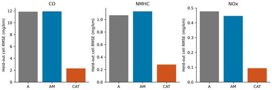
Adding ordinal mileage increased weighted training R² for every pollutant. However, CO LOCO MSE increased from 140.6490 under A to 141.8728 under AM, and NMHC increased from 1.1391 to 1.2753. NOx decreased from 0.22746 to 0.19948. The executed comparisons therefore demonstrated that the ordinal expansion improved training fit without consistently improving omitted-cell prediction.

Table 3 summarizes the specifications and their inverse-dispersion results. The R² ranges span the three pollutants; LOCO MSE is reported separately for each pollutant.

Table 3. Model specifications and inverse-dispersion performance within the 18-cell grid. Coefficient counts include the intercept; LOCO MSE is in (mg/km)².

Model	Specification	Number of Coefficients	Weighted R2 Range	LOCO MSE CO/NMHC/NOx
A	Age only	2	0.464–0.552	140.649/1.139/0.227
AM	Age, ordinal mileage, and interaction	4	0.608–0.615	141.873/1.275/0.199
CAT	Age, two mileage indicators, and age interactions	6	0.986–0.992	5.343/0.079/0.009

CAT achieved weighted R² values of 0.9920, 0.9860, and 0.9905 for CO, NMHC, and NOx, with LOCO MSE values of 5.3434, 0.0787, and 0.00883. Its reference predictions were 367.355, 18.085, and 7.362 mg/km. All full-data and deletion designs retained full column rank. At every age, category 2 means were below both category 1 and category 3 means for all three pollutants. CAT accommodated this nonmonotone pattern, whereas the ordinal specification restricted it. These observations explain the improved representation of the evaluated grid without establishing physical mileage thresholds or causal mechanisms. Figure 1 compares the LOCO RMSE across specifications.

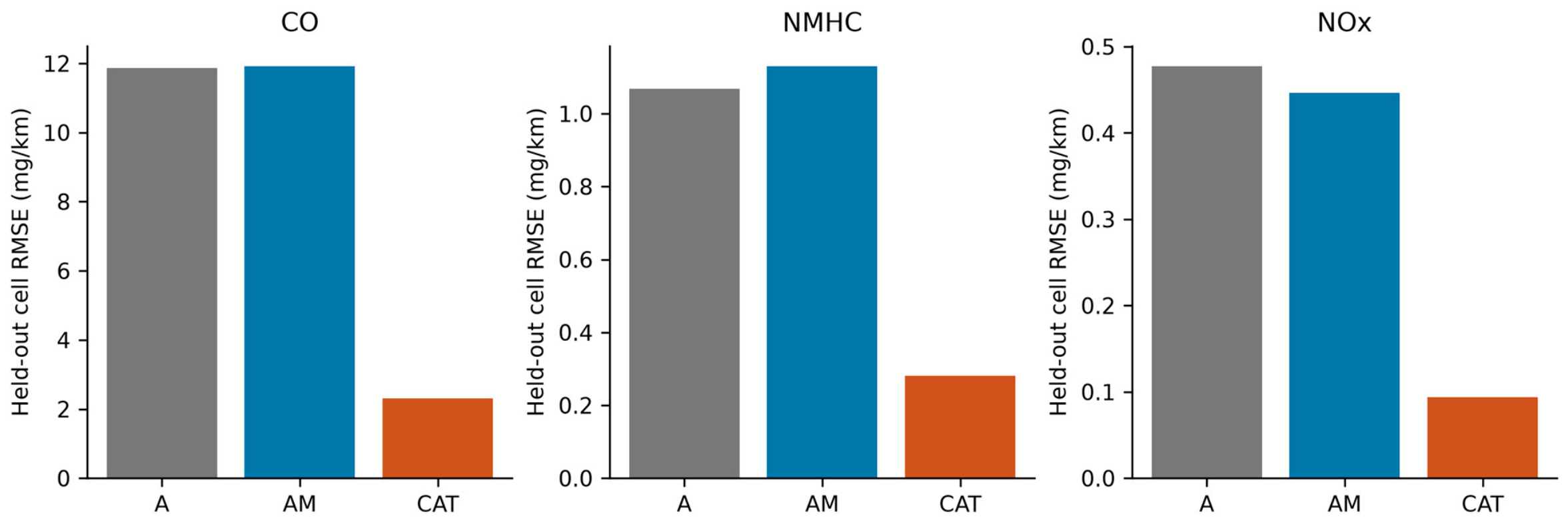
Figure 1. LOCO RMSE under inverse-dispersion weighting. A is age only, AM uses ordinal mileage, and CAT uses category indicators with age interactions. Pollutant panels have separate vertical scales. Bars summarize omitted grouped cells; no vehicle population uncertainty intervals are implied.

3.3. Weighting Conventions and Count Information

Count-informed AM produced reference estimates of 376.892, 18.939, and 7.727 mg/km and LOCO MSE values of 164.9040, 1.4796, and 0.23239. These errors exceeded the corresponding inverse-dispersion AM errors for all pollutants. The comparison evaluated equally weighted omitted-cell prediction, rather than sampling efficiency under a verified mean model. Count-informed CAT achieved substantially smaller LOCO MSE values of 5.3136, 0.0793, and 0.00892. The effective cell count, (∑w)²/∑w², summarized weight concentration; it was distinct from the reported count sum of 1000, whose interpretation as distinct vehicles was unverified. Table 4 reports on the weighting comparison.

Table 4. AM reference predictions and LOCO MSE from the weighting comparison. Count-informed weights use the reported counts in Table 1.

Pollutant	Weight Rule	Reference (mg/km)	LOCO MSE ((mg/km)2)	Effective Cell Count
CO	Equal	379.322	133.6090	18.00
CO	Inverse SD	378.941	137.3441	17.91
CO	Inverse dispersion	378.537	141.8728	17.66
CO	Count-informed	376.892	164.9040	16.22
NMHC	Equal	19.194	1.1821	18.00
NMHC	Inverse SD	19.147	1.2237	17.84
NMHC	Inverse dispersion	19.096	1.2753	17.38
NMHC	Count-informed	18.939	1.4796	15.89
NOx	Equal	7.820	0.18721	18.00
NOx	Inverse SD	7.806	0.19265	17.89
NOx	Inverse dispersion	7.790	0.19948	17.59
NOx	Count-informed	7.727	0.23239	16.16

3.4. Influence, Robust Regression, and Weight Sensitivity

The maximum absolute changes in the AM reference estimate after deleting one cell were 2.797 mg/km for CO, 0.279 mg/km for NMHC, and 0.110 mg/km for NOx. Maximum weighted leverages were 0.468, 0.481, and 0.473, respectively. All 648 linear deletion fits and 54 Huber deletion fits completed successfully, with no rank failures. The companion archive contains the complete deletion vectors and coefficient estimates. Table 5 summarizes the deletion and Huber diagnostics.

Table 5. AM deletion and residual robustness diagnostics under inverse-dispersion weights. Reference changes are in mg/km.

Pollutant	Maximum Absolute Reference Change	Omitted Cell	Maximum Leverage	Huber Reference	Huber LOCO MSE
CO	2.797	g17	0.468	382.934	175.7033
NMHC	0.279	g18	0.481	19.388	1.9481
NOx	0.110	g18	0.473	7.959	0.26833

Huber AM produced reference estimates of 382.934, 19.388, and 7.959 mg/km for CO, NMHC, and NOx, respectively. Its LOCO MSE exceeded that of inverse-dispersion WLS AM for every pollutant. Thus, Huber estimation did not improve omitted-cell prediction under ordinal-mileage coding. Residual robustness and correction of functional misspecification addressed different properties of the fitted model.

At ρ = 0, the attained ranges collapsed to the reference predictions. At ρ = 0.5, the ranges were 372.079–383.633 for CO, 18.509–19.588 for NMHC, and 7.547–7.983 mg/km for NOx. Across positive tolerances, 142 of 144 optimization runs converged and satisfied the feasibility threshold. Two CO minimization runs, one at ρ = 0.25 and one at ρ = 1, terminated with failure statuses and were excluded. Successful feasible runs determined the reported ranges. The largest constraint violation across all attempted runs was approximately 4.42 × 10⁻⁷; all accepted runs satisfied the feasibility tolerance of 10⁻⁷. These calculations established feasible attained sensitivity ranges under the implemented multistart procedure, without certifying global optimality. Table 6 reports the attained ranges.

Table 6. Approximate attained AM reference prediction ranges over bounded relative weight changes, in mg/km. These are not confidence intervals or certified global bounds.

Tolerance ρ	CO	NMHC	NOx
0.25	375.196 to 381.484	18.789 to 19.376	7.665 to 7.902
0.5	372.079 to 383.633	18.509 to 19.588	7.547 to 7.983
1.0	366.584 to 386.727	18.000 to 19.830	7.345 to 8.100

At ρ = 0, the attained ranges collapsed to the reference predictions. At ρ = 0.5, the ranges were 372.079–383.633 for CO, 18.509–19.588 for NMHC, and 7.547–7.983 mg/km for NOx. Across positive tolerances, 143 of 144 optimization runs converged and satisfied the feasibility threshold. One CO minimization started at ρ = 1, terminated with a failure status, and was excluded; successful starts determined the corresponding range. The largest constraint violation across all runs was below 1.6 × 10⁻⁹. These calculations established feasible attained sensitivity ranges under the implemented multistart procedure, without certifying global optimality. Table 6 reports on the attained ranges.

3.5. Simulation Results

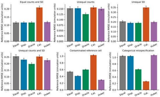
With equal counts and SD, the three linear AM weighting rules produced identical predictions and RMSE of 0.116. Under unequal counts alone, oracle count-informed AM achieved RMSE of 0.126, compared with 0.153 for inverse-dispersion AM. When counts and SD were both unequal, the corresponding values were 0.197 and 0.230. The controlled experiments demonstrated the benefit of count-informed weighting under the evaluated correctly specified mean model with known variances. Table 7 and Figure 2 summarize the simulation results.

Table 7. Reference prediction RMSE across six simulated scenarios. Each entry is RMSE (Monte Carlo SE), in simulation units, from 1000 repetitions.

Scenario	Equal AM	Dispersion AM	Oracle AM	Dispersion CAT	Huber AM
Equal counts and SD	0.116 (0.003)	0.116 (0.003)	0.116 (0.003)	0.209 (0.005)	0.119 (0.003)
Unequal counts	0.153 (0.003)	0.153 (0.003)	0.126 (0.003)	0.157 (0.003)	0.151 (0.004)
Unequal SD	0.206 (0.005)	0.190 (0.004)	0.190 (0.004)	0.349 (0.008)	0.199 (0.004)
Unequal counts and SD	0.256 (0.006)	0.230 (0.006)	0.197 (0.005)	0.254 (0.005)	0.226 (0.005)
Contaminated g17	0.542 (0.008)	0.414 (0.007)	0.603 (0.006)	1.030 (0.008)	0.298 (0.007)
Category 2 shift	1.049 (0.008)	1.043 (0.008)	0.633 (0.006)	0.264 (0.006)	1.071 (0.009)

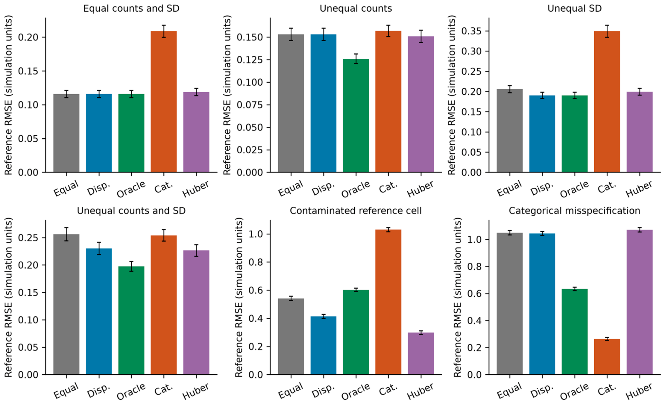
Figure 2. Simulation reference prediction RMSE. Error bars are approximately 95% Monte Carlo intervals, not confidence intervals for emission estimates. Disp. denotes inverse dispersion, Oracle uses known counts and variances, Cat. uses mileage categories, and Huber uses the AM design. Panels have separate vertical scales. Simulation units and targets are unrelated to the pollutant units in Figure 1.

Contamination changed the performance ordering: oracle AM RMSE increased to 0.603, compared with 0.298 for Huber AM and 0.414 for inverse-dispersion AM. With the category 2 mean shift, inverse-dispersion CAT achieved RMSE of 0.264, compared with 1.043 for inverse-dispersion AM and 1.071 for Huber AM. CAT also incurred a variance cost when the simpler mean model was correctly specified: its RMSE was 0.209 versus 0.116 for AM in the equal-count, equal-SD scenario. All 30,000 simulated fits completed successfully. These completed experiments quantified the distinct effects of precision weighting, residual contamination, and functional misspecification under the specified conditions.

3.6. Age-Level Validation and Covariance Sensitivity

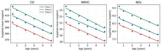
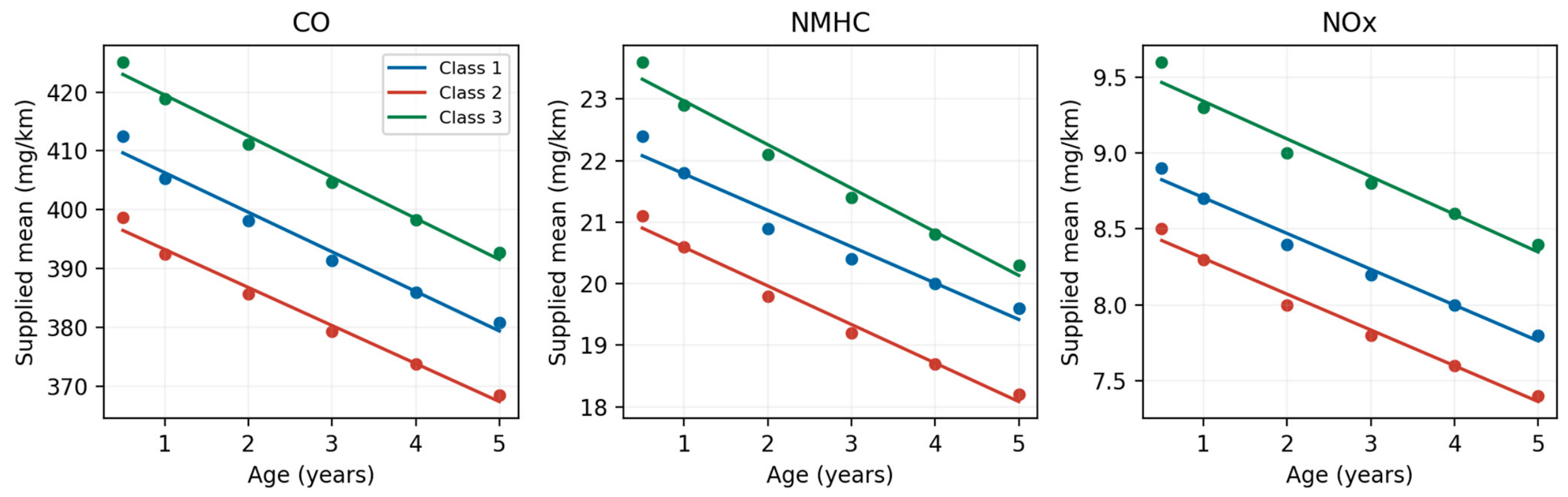
Table 8 reports age-level validation, and Figure 3 displays fitted CAT curves alongside all supplied means. CAT retains lower MSE than A and AM for every pollutant after withholding a complete age level. However, age-only models improve on their LOCO errors because all three mileage classes are jointly omitted rather than leaving isolated cross-class contrasts in a fold. CAT age-level and cell-level MSEs coincide with displayed precision: its design separates into three independently fitted age lines, so withholding the other two classes at the same age does not change the fitted line for an omitted class. This algebraic property limits the additional information provided by agreement of these validation results. The largest CAT fold MSE occurs when age 0.5 is withheld, emphasizing endpoint sensitivity. The result supports prediction across this supplied grid, including endpoint folds, while leaving external generalization untested.

Table 8. Leave-one-age-level-out MSE under inverse-dispersion weighting in (mg/km)². Each fold omits three cells; overall MSE gives equal weight to all 18 predictions.

Pollutant	A	AM	CAT	CAT Age 0.5 Fold	CAT Age 5 Fold
CO	115.77666	87.78526	5.34336	17.75162	8.03156
NMHC	0.95700	0.77959	0.07865	0.21886	0.13619
NOx	0.18784	0.12317	0.00883	0.02978	0.01001

Figure 3. Supplied cell means (points) and inverse-dispersion CAT fitted age lines by mileage class. All curves are fitted to the full supplied table, not held-out predictions. The middle-class dip is descriptive; units and mileage definitions retain the provenance limitations in Section 2.1.

Table 9 compares three covariance conventions for count-informed fits. For CAT, plug-in reference SEs exceed both residual-scale and HC3 SEs for all pollutants. For example, the CO CAT SE is 3.779 mg/km under the plug-in covariance versus 1.004 and 1.484 mg/km with residual scaling and HC3. The close fit of separate age lines yields small residual-based scales, whereas plug-in covariance retains the variance implied by the reported SDs and counts. None of these values verify population precision, and their disagreement is scientifically more informative here than choosing the smallest SE.

Table 9. Count-informed reference predictions and standard errors in mg/km. Plug-in covariance is unscaled and conditional on reported counts and dispersions; working covariance uses residual scaling.

Pollutant	Model	Reference	Working SE	HC3 SE	Plug-in SE
CO	A	376.4212	4.5177	4.7766	2.5532
CO	AM	376.8920	4.6111	5.7743	2.5813
CO	CAT	367.3090	1.0042	1.4839	3.7786
NMHC	A	18.9192	0.3978	0.4485	0.1555
NMHC	AM	18.9388	0.4172	0.5518	0.1577
NMHC	CAT	18.0776	0.1181	0.1716	0.2260
NOx	A	7.7014	0.1747	0.1821	0.0508
NOx	AM	7.7272	0.1711	0.2202	0.0515
NOx	CAT	7.3602	0.0403	0.0543	0.0753

3.7. Estimated Dispersion and Contamination Experiments

Table 10 and Table 11 report the additional simulation results with estimated and known dispersions, respectively. With estimated dispersions and a correctly specified ordinal mean, AM achieved a lower RMSE than CAT (0.205 versus 0.257). CAT reduced RMSE under both the middle-class dip and rise, whereas the monotone category modification produced similar errors for AM and CAT (0.242 and 0.250). Thus, the benefit of categorical coding depended on the underlying mean pattern. With +6 SD contamination at g17, RMSE increased to 0.591 for AM and 0.943 for CAT. Contamination at the two other evaluated locations had smaller effects on the estimated mean at g17. This location dependence qualified the findings from the original g17-only contamination scenario. Comparisons between known and estimated dispersions used paired sampled means, while separate random draws were used across scenarios. Small differences between methods should therefore be interpreted alongside their Monte Carlo standard errors.

Table 10. Reference prediction RMSE and nominal 95% interval coverage in the additional simulations with estimated dispersions. Monte Carlo standard errors (MCSEs) are reported in parentheses, and coverage is expressed as a percentage. Each scenario uses 1000 repetitions. Plug-in intervals use a normal critical value; working and HC3 intervals use t critical values with G − d degrees of freedom.

Scenario	Model	RMSE (MCSE)	Plug-in %	Working %	HC3%
Ordinal mean	AM	0.205 (0.005)	93.9	94.5	95.2
Ordinal mean	CAT	0.257 (0.006)	95.1	94.7	93.1
Monotone category mean	AM	0.242 (0.005)	89.7	96.7	96.4
Monotone category mean	CAT	0.250 (0.006)	95.6	95.5	92.6
Middle-class dip	AM	0.647 (0.007)	15.9	99.7	99.2
Middle-class dip	CAT	0.264 (0.006)	93.6	94.3	92.3
Middle-class rise	AM	0.643 (0.007)	16.5	99.9	99.5
Middle-class rise	CAT	0.252 (0.006)	95.2	95.8	92.9
g01 plus 3 SD	AM	0.217 (0.005)	93.1	95.8	95.6
g01 plus 3 SD	CAT	0.260 (0.006)	94.4	96.2	93.0
g01 plus 6 SD	AM	0.248 (0.005)	87.2	99.1	97.9
g01 plus 6 SD	CAT	0.259 (0.006)	94.4	99.2	91.9
g09 plus 3 SD	AM	0.219 (0.005)	92.4	97.6	96.8
g09 plus 3 SD	CAT	0.251 (0.006)	95.4	98.7	91.8
g09 plus 6 SD	AM	0.259 (0.005)	86.2	99.6	98.5
g09 plus 6 SD	CAT	0.248 (0.006)	94.7	99.9	94.2
g17 plus 3 SD	AM	0.347 (0.006)	69.2	85.4	96.1
g17 plus 3 SD	CAT	0.530 (0.008)	55.8	74.3	93.9
g17 plus 6 SD	AM	0.591 (0.007)	24.1	77.8	99.5
g17 plus 6 SD	CAT	0.943 (0.008)	6.7	55.3	99.7
Ordinal mean t5 errors	AM	0.202 (0.005)	93.9	93.9	95.9
Ordinal mean t5 errors	CAT	0.246 (0.006)	95.5	95.1	94.0

Table 11. RMSE and nominal 95% interval coverage for the estimated mean at age 5 and mileage class 2 in simulations with known dispersions. Monte Carlo standard errors (MCSEs) are reported in parentheses, and coverage is expressed as a percentage. Each scenario uses 1000 repetitions. Plug-in intervals use a normal critical value; working and HC3 intervals use t critical values with G − d degrees of freedom.

Scenario	Model	RMSE (MCSE)	Plug-in %	Working %	HC3%
Ordinal mean	AM	0.200 (0.004)	95.0	95.1	95.7
Ordinal mean	CAT	0.255 (0.006)	95.6	95.1	94.1
Monotone category mean	AM	0.238 (0.005)	91.4	96.6	96.6
Monotone category mean	CAT	0.248 (0.006)	95.2	95.0	93.1
Middle-class dip	AM	0.623 (0.006)	16.5	99.9	99.6
Middle-class dip	CAT	0.263 (0.006)	93.8	94.1	92.1
Middle-class rise	AM	0.621 (0.006)	15.5	100.0	99.8
Middle-class rise	CAT	0.251 (0.006)	95.7	95.4	93.9
g01 plus 3 SD	AM	0.214 (0.005)	94.0	95.7	95.7
g01 plus 3 SD	CAT	0.259 (0.006)	94.4	96.1	92.9
g01 plus 6 SD	AM	0.241 (0.005)	89.3	99.2	98.2
g01 plus 6 SD	CAT	0.257 (0.006)	95.1	99.3	92.4
g09 plus 3 SD	AM	0.211 (0.005)	94.6	98.0	97.3
g09 plus 3 SD	CAT	0.249 (0.006)	96.4	99.1	92.0
g09 plus 6 SD	AM	0.249 (0.005)	87.8	99.6	98.5
g09 plus 6 SD	CAT	0.247 (0.006)	94.9	99.9	94.3
g17 plus 3 SD	AM	0.349 (0.006)	69.0	84.7	95.9
g17 plus 3 SD	CAT	0.528 (0.008)	55.7	74.9	94.2
g17 plus 6 SD	AM	0.592 (0.006)	20.3	78.1	99.6
g17 plus 6 SD	CAT	0.932 (0.008)	5.0	56.1	99.7
Ordinal mean t5 errors	AM	0.200 (0.005)	94.5	94.2	95.7
Ordinal mean t5 errors	CAT	0.245 (0.006)	95.5	95.3	93.9

Interval coverage also varied with the mean pattern and covariance rule. Under the correctly specified ordinal mean with estimated dispersions, plug-in, residual-scaled, and HC3 coverage for AM was 93.9%, 94.5%, and 95.2%, respectively; CAT HC3 coverage was 93.1%. Under the middle-class dip, AM plug-in coverage fell to 15.9%, whereas residual-scaled and HC3 coverage reached 99.7% and 99.2%. These conservative coverage rates showed that residual-based intervals could conceal mean model misspecification through increased interval width. With +6 SD contamination at g17, CAT plug-in and residual-scaled coverage fell to 6.7% and 55.3%, while HC3 coverage reached 99.7%. Both undercoverage and conservative coverage therefore occurred across the evaluated scenarios. Heavy-tailed mean errors provided an additional stress condition, although cell independence remained an assumption throughout. No interval rule maintained nominal coverage across all scenarios.

3.8. Additive Categorical Comparison and Model Complexity

The additive categorical model substantially reduced prediction error relative to AM despite having the same number of coefficients (Table 12). Under inverse-dispersion weighting, ACAT also achieved lower LOCO MSE than CAT for all three pollutants. The age-blocked comparisons were mixed: CAT had slightly lower MSE for CO and NMHC, whereas ACAT had lower MSE for NOx. Adjusted R² favored ACAT for CO and NOx and CAT for NMHC. Thus, categorical coding captured features of the supplied mean pattern without requiring category-specific age slopes, while the additional interactions did not consistently improve prediction.

Table 12. Model complexity comparison under inverse-dispersion weighting. Prediction MSE gives equal weight to each held-out cell and is expressed in (mg/km)². Age-blocked validation withholds all three mileage categories at one age level.

Pollutant	Model	Coefficients	Adjusted R2	LOCO MSE	Age-Blocked MSE
CO	AM	4	0.5244	141.87284	87.78526
CO	ACAT	4	0.9897	3.37032	5.46747
CO	CAT	6	0.9887	5.34336	5.34336
NMHC	AM	4	0.5261	1.27528	0.77959
NMHC	ACAT	4	0.9795	0.05855	0.08507
NMHC	CAT	6	0.9801	0.07865	0.07865
NOx	AM	4	0.5320	0.19948	0.12317
NOx	ACAT	4	0.9882	0.00565	0.00857
NOx	CAT	6	0.9866	0.00883	0.00883

ACAT also produced smaller HC3 standard errors for the reference estimate than CAT: 1.019 versus 1.514 mg/km for CO, 0.114 versus 0.173 mg/km for NMHC, and 0.034 versus 0.055 mg/km for NOx. Its maximum reference estimate change under single-cell deletion was smaller for all three pollutants, although this ordering did not hold under age-level deletion. These results support distinguishing the benefit of categorical coding from the benefit of adding age interactions. The comparisons remain exploratory assessments within the supplied grid.

3.9. Correlated Errors and Count Input Uncertainty

Positive correlation between cells within the same mileage category increased estimation variability and reduced interval coverage (Table 13). For AM, RMSE increased from 0.210 under independence to 0.291 at correlation 0.6, while HC3 coverage decreased from 94.8% to 77.1%. For CAT, the corresponding RMSE increased from 0.266 to 0.370, and HC3 coverage decreased from 91.1% to 67.5%. Thus, accounting for heteroskedasticity through HC3 did not adequately account for the simulated dependence.

Table 13. Sensitivity to correlated cell errors and perturbed count inputs. Each row summarizes 1000 repetitions using estimated dispersions. Bias, empirical SD, and RMSE concern the estimated mean at age 5 and mileage class 2 and are expressed in simulation units. RMSE Monte Carlo standard errors appear in parentheses. Coverage is expressed as a percentage. Correlation applies within mileage categories; count CV denotes the coefficient of variation of the multiplicative count perturbation before rounding.

Scenario	Model	Bias	Empirical SD	RMSE (MCSE)	Plug-In %	Working %	HC3%
Independent	AM	−0.007	0.210	0.210 (0.005)	93.8	93.7	94.8
Independent	ACAT	−0.019	0.218	0.219 (0.005)	92.3	93.8	94.9
Independent	CAT	−0.008	0.266	0.266 (0.006)	93.1	94.5	91.1
Correlation 0.3	AM	−0.020	0.256	0.257 (0.005)	86.4	84.2	88.2
Correlation 0.3	ACAT	−0.035	0.267	0.269 (0.006)	85.8	82.6	84.9
Correlation 0.3	CAT	−0.025	0.323	0.324 (0.007)	87.7	83.3	82.3
Correlation 0.6	AM	−0.025	0.290	0.291 (0.006)	80.7	73.6	77.1
Correlation 0.6	ACAT	−0.040	0.304	0.306 (0.007)	78.2	67.3	72.5
Correlation 0.6	CAT	−0.031	0.369	0.370 (0.008)	82.6	64.2	67.5
Count CV 0.25	AM	−0.005	0.212	0.212 (0.005)	93.2	93.4	94.9
Count CV 0.25	ACAT	−0.017	0.221	0.222 (0.005)	91.4	94.0	94.8
Count CV 0.25	CAT	−0.006	0.270	0.269 (0.006)	93.0	94.5	91.3
Count CV 0.50	AM	−0.003	0.222	0.222 (0.005)	91.8	91.7	94.8
Count CV 0.50	ACAT	−0.014	0.232	0.233 (0.005)	90.5	92.1	94.4
Count CV 0.50	CAT	−0.004	0.280	0.280 (0.006)	92.2	92.9	90.4
Correlation 0.3 + count CV 0.50	AM	−0.015	0.267	0.268 (0.006)	84.5	82.4	87.5
Correlation 0.3 + count CV 0.50	ACAT	−0.030	0.279	0.281 (0.006)	83.1	79.6	85.5
Correlation 0.3 + count CV 0.50	CAT	−0.021	0.335	0.335 (0.008)	86.6	79.9	80.8

Count perturbations alone produced smaller changes under the evaluated settings. At a count-multiplier coefficient of variation of 0.50, AM and CAT RMSEs were 0.222 and 0.280, respectively. Combining this perturbation with a correlation of 0.3 increased RMSE to 0.268 and 0.335. Empirical standard deviations were close to the corresponding RMSEs, indicating that variability accounted for most of the estimation error in these scenarios. The base mean included an age–mileage interaction, which AM and CAT could represent but ACAT could not represent exactly. These results distinguish sensitivity to dependence from sensitivity to the count inputs and do not identify the sampling structure underlying the supplied emission summaries.

4. Discussion

4.1. Grouped-Input Findings and Methodological Implications

The comparisons on the supplied grouped table identified mileage representation as the dominant modeling choice in the grouped dataset. Ordinal mileage increased training but worsened LOCO prediction for CO and NMHC. Categorical mileage represented the category 2 dip and substantially reduced omitted-cell errors. Alternative weighting and Huber estimation did not achieve a comparable reduction while retaining the ordinal mean structure. The calculated advantage therefore arose primarily from relaxing the functional restriction rather than introducing a different loss or weighting convention.

The four weighting methods answer different operational questions. Equal weights target average performance over the 18 supplied cells; inverse-SD and inverse-dispersion weights progressively reduce the influence of cells with larger reported within-cell spread; count-informed weights additionally favor reported larger cells. In AM, the count-informed reference prediction is lower and equal-cell LOCO error is higher than under inverse dispersion for all pollutants (Table 4). This does not refute precision weighting under correct sampling assumptions: its objective differs from equal-cell prediction, and the ordinal mean is restrictive. In practice, an analyst seeking a representative fleet estimate would first need verified counts and fleet composition. For a descriptive comparison of supplied cells, equal-cell validation is directly interpretable. Reported count-informed results should remain a sensitivity analysis until the counts are reconciled [26].

4.2. Uncertainty and Generalization

The explicit covariance comparison in Table 9 shows why small CAT residual-based SEs require caution: close agreement with a smooth supplied table does not establish precise population sampling. Table 10 and Table 11 add coverage under constructed data-generating mechanisms with both known and estimated dispersions. Coverage varies markedly with misspecification, contamination location, and covariance convention. HC3 adjusts residual contributions for leverage but neither guarantees nominal coverage at G = 18 nor repairs an incorrect reference mean. The six-coefficient CAT model uses a substantial fraction of the available cell-level information [27]. Independence, count validity, and the meaning of the reported SDs remain unverified for Table 1; the simulation cannot supply those missing facts.

LOCO and age-level validation assess different omissions within the same supplied grid (Table 8). The latter withholds all mileage classes at an age and includes endpoint extrapolation folds, but the common design and separate-line structure of CAT limit its independence from LOCO. Neither procedure tests an independent fleet, a new measurement program, unobserved mileage classes, or individual vehicle prediction. Exploratory selection based on these comparisons requires independent confirmation [9]. The decline of supplied means with age and the lower middle-mileage means must not be read as physical deterioration, protective mileage effects, or fleet trends. Vehicle technology, maintenance, fuel type, test conditions, selection, and cohort composition may confound or even reverse these descriptive associations [28]. No causal age or mileage effect is identified.

4.3. Data Limitations and Extensions

The principal unresolved limitation is measurement provenance. The source manuscript describes a 445-test JRC program, whereas the supplied count column sums to 1000 and its assignment frequencies disagree in 17 cells. These discrepancies cannot be reconciled by statistical reweighting. The original aggregation records, unique vehicle and test identifiers, repeated-test mapping, unit conversions, mileage cutoffs, measurement dates, and within-cell SD definitions are required to establish a characterized sample. Until then, Table 1 is an auditable computational input rather than verified fleet evidence. The supplied workbooks and their documentation distinguish the grouped summaries, generated observations, resampled emissions, and JRC test records. However, they do not establish a verified record-level derivation of Table 1. The computational inputs, analysis code, and verification records are provided in the accompanying GitHub repository.

We did not apply a cold-start multiplier to the emission estimates. The measurement-phase boundary was not verified, and no pollutant-specific 7% contribution was made. Applying such a multiplier to a quantity that already includes cold-start emissions would double-count that contribution. This unresolved physical definition limits phase-specific interpretation without changing the regression and simulation experiments completed here.

DRO [29] and multi-pollutant partial pooling [30] were not components of the evaluated pipeline. Extending the work to these models would require complete estimation specifications, appropriate assumptions, and comparisons against the implemented baselines. EPA manufacturer-run in-use testing data provides a candidate for a separate external evaluation after harmonizing vehicle classes, units, pollutant definitions, and test procedures [31]. Such records should not be assumed to be the source of the present grouped table.

5. Conclusions

This computational case study shows how weighting, mileage coding, and covariance assumptions can lead to different conclusions from the same 18 supplied emission summary cells. Categorical mileage predicts the supplied grid better than ordinal mileage in cell- and age-level omissions because it represents the middle-class dip. Additional simulations show that this advantage is conditional: an ordinal model can have lower errors when correctly specified, and contamination at the reference cell can strongly harm CAT predictions. Estimated dispersions and the choice of interval rule also affect reference mean coverage. The practical implication is to define the estimation target, inspect the mean structure, compare predictive losses under explicit validation schemes, and report covariance sensitivity rather than rely on training fit or the smallest SE. These calculations establish the behavior of supplied summaries and constructed mechanisms. They do not establish causal age or mileage effects, population-level precision, or results for a verified JRC sample. Traceable measurement records, reconciled counts, and independent external evaluation remain necessary for fleet-level conclusions.

References

- Romano, J.P.; Wolf, M. Resurrecting weighted least squares. J. Econom. 2017, 197, 1–19. [Google Scholar] [CrossRef] [Scilit]
- Harrell, F.E., Jr. Regression Modeling Strategies: With Applications to Linear Models, Logistic and Ordinal Regression, and Survival Analysis, 2nd ed.; Springer: Berlin/Heidelberg, Germany, 2015. [Google Scholar] [CrossRef] [Scilit]
- Cawley, G.C.; Talbot, N.L.C. On over-fitting in model selection and subsequent selection bias in performance evaluation. J. Mach. Learn. Res. 2010, 11, 2079–2107. [Google Scholar]
- Arlot, S.; Celisse, A. A survey of cross-validation procedures for model selection. Stat. Surv. 2010, 4, 40–79. [Google Scholar] [CrossRef] [Scilit]
- Roberts, D.R.; Bahn, V.; Ciuti, S.; Boyce, M.S.; Elith, J.; Guillera-Arroita, G.; Hauenstein, S.; Lahoz-Monfort, J.J.; Schröder, B.; Thuiller, W.; et al. Cross-validation strategies for data with temporal, spatial, hierarchical, or phylogenetic structure. Ecography 2017, 40, 913–929. [Google Scholar] [CrossRef] [Scilit]
- Varoquaux, G. Cross-validation failure: Small sample sizes lead to large error bars. NeuroImage 2018, 180, 68–77. [Google Scholar] [CrossRef] [Scilit] [PubMed]
- Huber, P.J. Robust estimation of a location parameter. Ann. Math. Stat. 1964, 35, 73–101. [Google Scholar] [CrossRef] [Scilit]
- Morris, T.P.; White, I.R.; Crowther, M.J. Using simulation studies to evaluate statistical methods. Stat. Med. 2019, 38, 2074–2102. [Google Scholar] [CrossRef] [Scilit] [PubMed]
- Bates, S.; Hastie, T.; Tibshirani, R. Cross-validation: What does it estimate and how well does it do it? J. Am. Stat. Assoc. 2024, 119, 1434–1445. [Google Scholar] [CrossRef] [Scilit] [PubMed]
- European Commission, Joint Research Centre. Light-Duty Vehicle Exhaust Emissions: On-Road Testing Data in Support to Euro 7 Regulation [Dataset]. Joint Research Centre: European Commission, 2024. Available online: https://doi.org/10.2905/JRC.8897YXR (accessed on 5 September 2026). [CrossRef]
- European Commission, Directorate-General for Internal Market, Industry, Entrepreneurship and SMEs. Technical Studies for the Development of Euro 7: Durability of Light-Duty Vehicle Emissions; Publications Office of the European Union: Luxembourg, 2022. [Google Scholar] [CrossRef] [PubMed]
- U.S. Environmental Protection Agency. Dynamometer Drive Schedules. Available online: https://www.epa.gov/vehicle-and-fuel-emissions-testing/dynamometer-drive-schedules (accessed on 15 October 2026).
- Gelman, A.; Hill, J. Data Analysis Using Regression and Multilevel/Hierarchical Models; Cambridge University Press: Cambridge, UK, 2007. [Google Scholar] [CrossRef] [Scilit]
- Seber, G.A.F.; Lee, A.J. Linear Regression Analysis, 2nd ed.; Wiley: Hoboken, NJ, USA, 2003. [Google Scholar] [CrossRef] [Scilit]
- Winship, C.; Radbill, L. Sampling weights and regression analysis. Sociol. Methods Res. 1994, 23, 230–257. [Google Scholar] [CrossRef] [Scilit]
- MacKinnon, J.G.; White, H. Some heteroskedasticity-consistent covariance matrix estimators with improved finite sample properties. J. Econom. 1985, 29, 305–325. [Google Scholar] [CrossRef] [Scilit]
- Long, J.S.; Ervin, L.H. Using heteroscedasticity consistent standard errors in the linear regression model. Am. Stat. 2000, 54, 217–224. [Google Scholar] [CrossRef] [Scilit]
- Cook, R.D. Detection of influential observation in linear regression. Technometrics 1977, 19, 15–18. [Google Scholar] [CrossRef] [Scilit]
- Stone, M. Cross-validatory choice and assessment of statistical predictions. J. R. Stat. Soc. Ser. B (Methodol.) 1974, 36, 111–133. [Google Scholar] [CrossRef] [Scilit]
- Huber, P.J.; Ronchetti, E.M. Robust Statistics, 2nd ed.; Wiley: Hoboken, NJ, USA, 2009. [Google Scholar] [CrossRef] [Scilit]
- Nocedal, J.; Wright, S.J. Numerical Optimization, 2nd ed.; Springer: Berlin/Heidelberg, Germany, 2006. [Google Scholar] [CrossRef] [Scilit]
- Bertsimas, D.; Brown, D.B.; Caramanis, C. Theory and applications of robust optimization. SIAM Rev. 2011, 53, 464–501. [Google Scholar] [CrossRef] [Scilit]
- Peng, R.D. Reproducible research in computational science. Science 2011, 334, 1226–1227. [Google Scholar] [CrossRef] [Scilit]
- Sandve, G.K.; Nekrutenko, A.; Taylor, J.; Hovig, E. Ten simple rules for reproducible computational research. PLoS Comput. Biol. 2013, 9, e1003285. [Google Scholar] [CrossRef] [Scilit] [PubMed]
- Groth, P.; Moreau, L. (Eds.) PROV-Overview: An Overview of the PROV Family of Documents. W3C Working Group Note, 30 April 2013. 2013. Available online: https://www.w3.org/TR/prov-overview/ (accessed on 15 October 2026).
- Solon, G.; Haider, S.J.; Wooldridge, J.M. What are we weighting for? J. Hum. Resour. 2015, 50, 301–316. [Google Scholar] [CrossRef] [Scilit]
- Hayes, A.F.; Cai, L. Using heteroskedasticity-consistent standard error estimators in OLS regression: An introduction and software implementation. Behav. Res. Methods 2007, 39, 709–722. [Google Scholar] [CrossRef] [Scilit] [PubMed]
- Hernán, M.A.; Robins, J.M. Causal Inference: What If; Chapman & Hall/CRC: Boca Raton, FL, USA, 2020; Available online: https://miguelhernan.org/whatifbook (accessed on 15 October 2026).
- Ben-Tal, A.; den Hertog, D.; De Waegenaere, A.; Melenberg, B.; Rennen, G. Robust solutions of optimization problems affected by uncertain probabilities. Manag. Sci. 2013, 59, 341–357. [Google Scholar] [CrossRef] [Scilit]
- Gelman, A. Prior distributions for variance parameters in hierarchical models. Bayesian Anal. 2006, 1, 515–533. [Google Scholar] [CrossRef] [Scilit]
- U.S. Environmental Protection Agency. Manufacturer-Run in-Use Testing Program Data for Light-Duty Vehicles, Light-Duty Trucks, and Heavy-Duty Vehicles Class 2b and 3. 2026. Available online: https://www.epa.gov/compliance-and-fuel-economy-data/manufacturer-run-use-testing-program-data-light-duty-vehicles (accessed on 15 October 2026).
- European Commission, Directorate-General for Internal Market, Industry, Entrepreneurship and SMEs. Technical Studies for the Development of Euro 7: Testing, Pollutants and Emission Limits; Publications Office of the European Union: Luxembourg, 2022. [Google Scholar] [CrossRef]
- U.S. Environmental Protection Agency. Compliance and Fuel Economy Data for Vehicles and Engines. Available online: https://www.epa.gov/compliance-and-fuel-economy-data (accessed on 15 October 2026).
Disclaimer/Publisher’s Note: The statements, opinions and data contained in all publications are solely those of the individual author(s) and contributor(s) and not of MDPI and/or the editor(s). MDPI and/or the editor(s) disclaim responsibility for any injury to people or property resulting from any ideas, methods, instructions or products referred to in the content. |
© 2026 by the authors. Licensee MDPI, Basel, Switzerland. This article is an open access article distributed under the terms and conditions of the Creative Commons Attribution (CC BY) license.