


Abstract
Many animal species have unique patterns on their body that allow for individual identification, and these patterns often have a genetic basis. This individual-level pattern variation can be leveraged in ecological applications in a number of ways, such as facilitating the identification of individuals in mark-recapture study systems, and informing conservation efforts by identifying the source populations of animals trafficked in the wildlife trade, for example. We tested four convolutional neural network architectures that researchers with access to training data can use to extract features for clustering individuals into a known number of biologically relevant groups in species with unique individual patterns. We used a common freshwater turtle species, the painted turtle (Chrysemys picta), which has intricate individual-level variation in plastron pattern. We compared the ability of our neural network approaches, traditional geometric morphometric methods, and software for identifying individuals to group individuals by clutch and population using two clustering methods. We found that no methods reliably recovered clutch membership (i.e., half or full siblings) from plastron patterns (Adjusted Rand indices < 0.266). However, individuals could be sorted into source populations with high agreement using both methods, with the convolutional autoencoder resulting in the best clustering (Adjusted Rand index = 0.858). Most of our neural network approaches outperformed (had higher Adjusted Rand indices than) the geometric morphometric methods in both cases, and both of these approaches outperformed the similarity scores calculated by the individual identification software. These results demonstrate that neural-network-derived image features can provide an effective approach for evaluating whether uniquely identifiable individuals cluster into biologically relevant groups.
1. Introduction
Animal patterns have long been used by researchers for individual identification, and they can provide valuable information for long-term studies on wild populations. Body markings and patterns can have multiple functions for animals, including crypsis, predator deterrence, mate attraction, and individual recognition, and may sometimes be under opposing selective pressures. The specific patterns thus may have impactful direct or indirect impacts on fitness. For example, the size and shape of the spotted patterns on juvenile giraffes have been found to be highly correlated with survival [1]. In some cases, the unique patterns themselves may not be adaptive, such as the arrangement of collagen-elastin bundles in bat wings [2], or the shape of the unpigmented spot on koala noses [3]. Yet studying individual-level variation in patterns may provide valuable ecological and conservation information about their respective systems if pattern type is genetically linked. Thus, the development of a novel and reliable method for extracting pattern features from individual photographs would be extremely useful.
Typically, organisms are more genetically similar to others near their geographic location or within the same population, than to those that are more distant [4]. Thus, we can expect that, even for visually complex visual patterns under some genetic control, whether themselves adaptive or not, variation could be identifiable at the population level. Despite advancements in genetic technologies, long-term studies of wild populations often face issues that can make it hard to determine the genetic relatedness of many or most individuals in a population (e.g., high costs of molecular work, limited sample sizes, inability to observe mating or offspring rearing, etc.). Animal patterns may be leveraged in a unique way to provide an alternative means of relatedness information [5]. Often, numerous individual-level photographs are taken during the experimental process of many studies, across taxa, but those photographs are not typically being used for pattern variation analysis. Additionally, to date, existing software packages for pattern analysis have primarily focused on matching individuals for identification purposes [5,6], rather than extracting, quantifying, or grouping patterns. Thus, the ability of these types of patterns to be applied to population-based estimates of heredity or relatedness, has been underexplored.
Deep machine learning is an increasingly important tool for ecological studies [7,8,9] and may be useful for addressing the issues discussed above. Deep machine learning relies on interconnected groups of nodes known as artificial neural networks (ANNs) to analyze data for a variety of use cases. Artificial neural networks have been widely applied recently in ecology and wildlife biology for environmental monitoring, behavioral studies, or population genomics work, among other applications [8], and are a good fit for analyzing complex patterns in animals because they can extract fine-scale features. Models undergo iterative training, during which the model is fed training data, its output is compared to the true labels/values, and a measurement of error is calculated using a loss function. The model is optimized each iteration to improve output predictions. This process is repeated on each batch of data, which helps improve inference accuracy [10,11]. These networks can act as useful tools for analyzing and extracting complex animal patterns. Currently, convolutional neural networks (CNNs) are the most widely used neural architecture for image-based analyses in ecology [8].
Here, we use four neural network architectures and traditional geometric morphometric methods to extract pattern features from a wild freshwater turtle species with unique individual patterns. We then (1) compare the ability of these two approaches to recover biologically relevant groups (source populations and clutch-mates) to that of an existing software that scores similarity, using unsupervised clustering methods, and (2) discuss the relative utility of different representations of animal patterns for identifying such groups. The remainder of this paper is organized as follows. In Section 2, we review the study species, the methods of collecting images, the geometric morphometric approaches, the cluster analysis, the neural network feature extraction methods, the methods for extracting information from an existing identification software, and finally, how to then quantify the clustering success of each of these approaches. We also include our permits and animal use protocols in Section 2.8. Then in Section 3, we present the results of the clutch classifications and the population classifications. In Section 4, we discuss the utility of the different approaches, their possible biological drivers, the limitations of the approaches, the benefits of the approaches, and potential future applications. We then conclude the paper in Section 5 by stating our main conclusions.
2. Materials and Methods
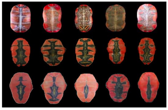
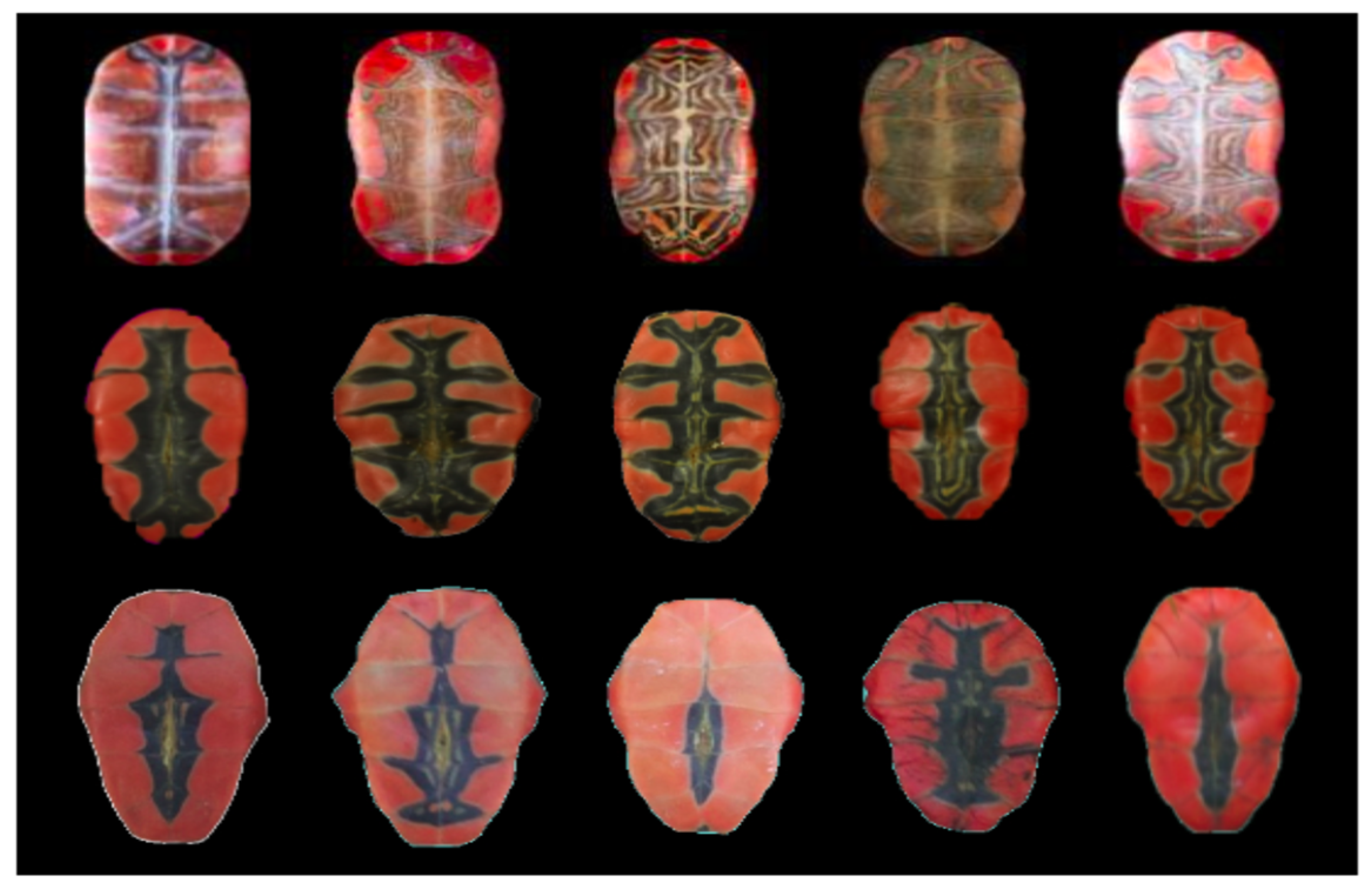
We used a commonly studied species of wild animal with uniquely identifiable body patterns (Figure 1) to test four neural network architectures for extracting pattern information. We then compared the abilities of the neural network architectures and a more traditional geometric morphometric method for analyzing patterns to recover clutch-mates (i.e., half and full siblings) and source populations.
Figure 1.
The isolated plastrons of painted turtles from northern Wisconsin (top row; used as training data), Thomson (middle row), and Barrington (bottom row).
2.1. Study Species
Painted turtles, Chrysemys picta, are a widespread freshwater turtle species in North America. Because of their abundance and distribution, painted turtles are the subject of multiple long-term studies, e.g., refs. [12,13,14,15], and photographs are sometimes used for secondary identification of individuals [13]. Most populations of this species have widely variable patterns on the plastron, or ventral portion of the shell [16]. These patterns are sufficiently variable to be reliably used for individual identification, which is especially useful for hatchlings who are too small and pliable for microchipping or shell notching. Painted turtles spend most of their time in lakes and slow-moving rivers with dense aquatic vegetation, but female turtles venture on land in early summer to lay eggs in a cavity they excavate and rebury [17]. Maternity can therefore be determined by excavating eggs from a nest in which a female is seen laying. However, all hatchlings from a nest may not be full siblings because this species exhibits multiple paternity [18]. Identifying paternity in this species can be especially logistically challenging and cost-prohibitive because populations sometimes consist of hundreds or thousands of individuals ranging over large geographic areas, and this species can store sperm across years [18,19]. Currently, there is nothing known about the heritability of the plastron pattern but it is presumed to be under at least some genetic control due to the high similarity of plastron patterns within clutches (this study, unpublished data), and the high amount of variation within populations [20]. Individuals maintain their plastron patterns from hatching throughout their decades of life [13], and thus a method to reliably group a large number of individuals by parentage using this pattern is feasible and could be extremely useful for long-term studies.
2.2. Image Collection
We photographed turtles from two different populations in Illinois, approximately 120 miles apart (see examples in Figure 1). In the Barrington population, nests (n = 18) were protected from predation using chicken wire cages after females finished nesting in May. This population was located entirely on a private pond and likely consisted of hundreds of individuals. In early autumn, the cages were removed and the plastrons of the hatched turtles (n = 141) were photographed outdoors using a Nikon DSLR camera before being released into the nearby pond. The other population is the site of a long-term mark-recapture study of this species at the Thomson Causeway Recreation Area, see refs. [15,21], comprising at least a thousand individuals across a wide geographic area on the Mississippi River [19]. Here, eggs were excavated from 30 nests after being laid and were taken to Michigan State University for incubation and overwintering as part of other experiments. Upon hatching in August, each individual plastron was photographed under identical indoor lighting conditions (n = 243). Knowing the source nests enabled classification of images of the hatchling plastrons by both population, and clutch (i.e., half or full sibling groups). We tested our clutch clustering methods on both populations separately and combined because the population sizes are so different that the genetic variation within each may differ as well.
2.3. Geometric Morphometric Methods
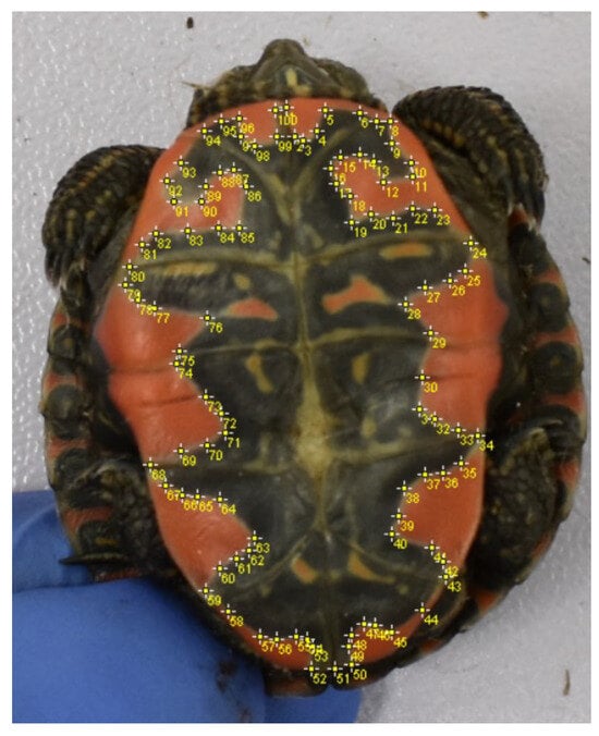
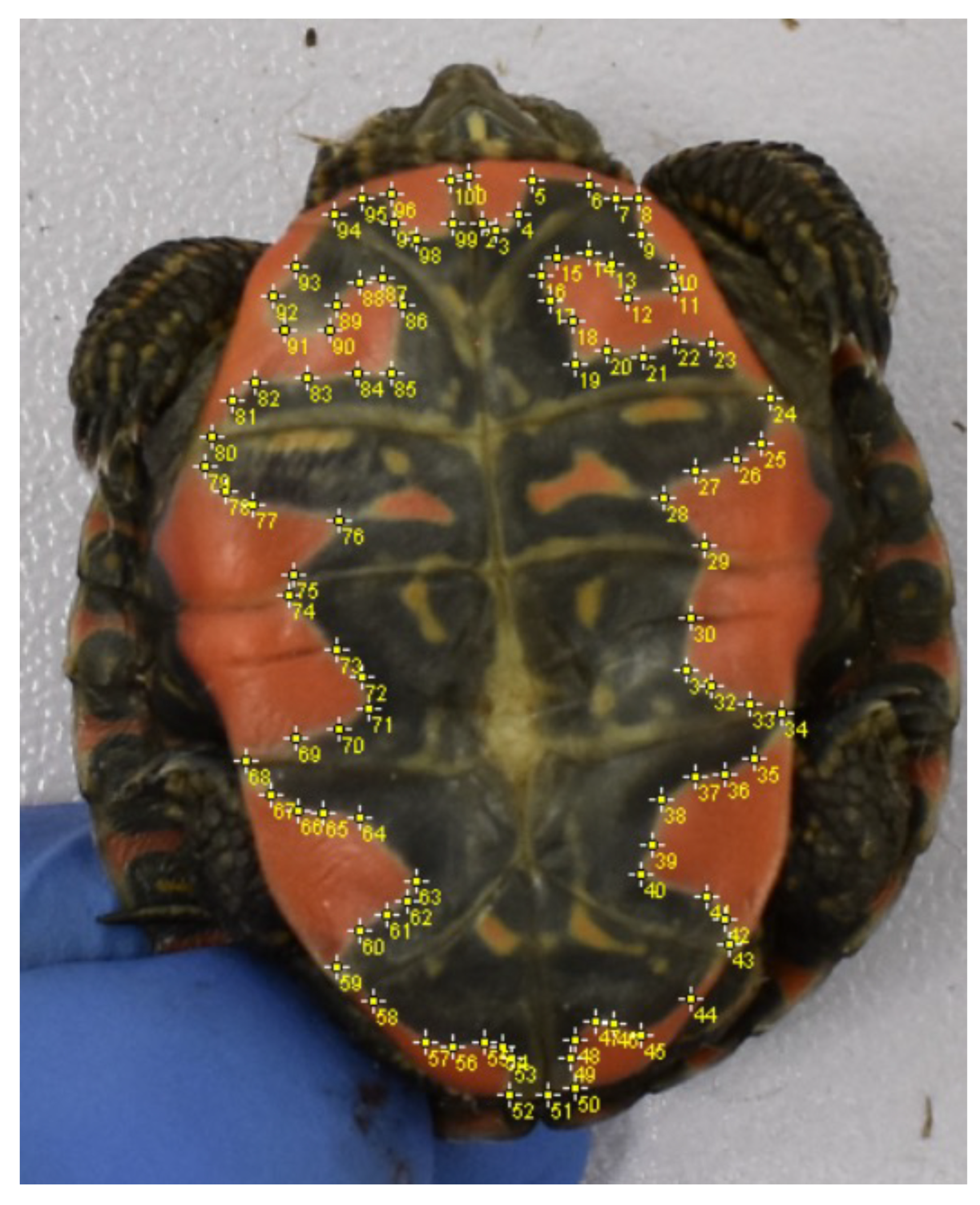
Deep learning is well-suited for working with complex patterns that may not be recognizable or quantifiable, but results can and should still be compared to baseline data collected without deep learning [8]. We sought to manually quantify plastron patterns using several geometric traits, and then used geometric morphometric approaches to compare the results of clustering to those obtained from features extracted by deep learning. To measure traits, we used ImageJ (v1.54g, Wayne Rasband and contributors, National Institutes of Health, Bethesda, MD, USA) [22] to manually place 100 points around the perimeter of the plastron pattern of each individual (Supplementary Material: Data S1). Care was taken to distribute points approximately equally along each side of the pattern, and to ensure that connecting them with straight lines would approximate the actual pattern as closely as possible (Figure 2).
Figure 2.
The outline of the pattern of the plastron (ventral shell) of painted turtle (Chrysemys picta) hatchlings was collected using 100 points. The distances from the centrum were then calculated, as was the percent area of the plastron occupied by the pattern, the solidity, and the convexity. The points were also used to conduct a shape principal component analysis.
We also placed points around the entire plastron to allow for quantifying the pattern area as a percentage of the plastron space it occupies (percent area). In order to compare the plastron shape of different turtles independent of the scale of the pictures and/or the orientation of the turtle in the pictures, we performed a Procrustes superimposition, i.e., we scaled and rotated the 100 points such that the first point is always mapped to the point (0,1), and the fifty-first point is always mapped to the point (0,−1). The Procrustes superimposition ensures that 100 points taken from two different pictures of the same turtle would have identical outputs. Moreover, the shapes of the plastron of several turtles can be plotted on a 2 × 2 square centered at the origin for an easy graphical comparison. After Procrustes superimposition, we calculated the centrum of the 100 points, and measured the distances between the centrum and each point to obtain a multivariate distance measurement. We also measured the solidity and convexity of the plastron patterns, two measurements commonly used in complex shape analysis. Convexity is calculated by measuring the perimeter of the convex hull created by the plastron pattern and dividing that by the overall perimeter of the plastron pattern. Solidity is calculated by measuring the area of the plastron pattern and dividing that by the area of the convex hull of the plastron pattern. Next, we performed a shape principal component analysis using the ‘shapepca’ function in the geomorph package [23]. We used the set of principal components that explained 99% of the variation for subsequent analyses. All analyses were performed in the R Statistical Programming Language (R Version 4.5.2, The R Foundation for Statistical Computing, Vienna, Austria) [24].
2.4. Cluster Analysis of GMM Pattern Analysis
We next tested two clustering algorithms on the following seven traits measured for each turtle: multivariate distance, the statistical summary of the multivariate distances, percent area, solidity, convexity, a multivariate trait that incorporated all of the aforementioned traits except the statistical summary, and the shape principal components. The multivariate distance was obtained by measuring the distances of the 100 Procrustes superimposed points from the centrum. The statistical summary included the standard deviation of these distances. The percent area was calculated as the ratio between the area of the plastron pattern and the area of the entire plastron. We used both k-means and hierarchical clustering for each trait, implemented in R. The k-means clustering used 1000 iterations, while the hierarchical clustering was deployed with the Euclidean distance and the Ward linkage method. This necessitated inputting the number of clusters to implement (clutch analysis: Barrington population: n = 18, Thomson population: n = 30, combined populations: n = 48; population analysis: n = 2). We used these same numbers to trim the trees produced with the hierarchical clustering approach to the appropriate number of branches in order to extract the clusters.
2.5. Neural Network Feature Extraction and Cluster Analysis
To reduce computational time and to focus on only the relevant aspects of the images, we first cropped images to only include the plastron, excluding the background, head, and limbs of the turtle, using a CNN-based segmentation network trained specifically on our turtle photos. For both training and testing, we isolated the plastral pattern from the rest of the image. We used a segmentation network to generate a mask of the plastral pattern, then extracted that region from the image. Some patterns were not accurately isolated by the segmentation network, in which case the pattern was cropped by hand. Finally, to avoid color variation caused by lighting, we converted all training and testing data into grayscale versions (Figure S1). We then set each image to dimensions of 128 × 64 pixels and compressed each image into an embedding space that was one-third of the original feature space using the TensorFlow library and a convolutional layer schema. This size was chosen to preserve information since the autoencoder and segmentation network downsize the image dimensions at each layer; this size preserved even the smallest of our images throughout the process. A training dataset was constructed using images of plastrons from northern Wisconsin, a different population than the two described above (Supplementary Material: ImageFiles). As in the main populations, photographs were taken of the plastrons of turtles in controlled outdoor conditions using a Nikon DSLR camera. However, this population consisted of mainly adults rather than hatchlings. Training images were similarly cropped, converted to gray scale, and placed on a 128 × 64 pixel canvas. Our autoencoder networks were trained on a dataset of 384 training images. Our segmentation network was trained using 303 images and their labels for the training set, and 81 images and their labels for the validation set.
Deep feature spaces (DFS) are reduced data extracted from images and used by the model. We tested four different DFS types. The first two DFS types were extracted from a fully connected autoencoder and a convolutional autoencoder model. Both model architectures consist of an encoder and decoder. The fully connected encoder comprises an initial flattened layer to bring our feature space from the original input shape of 128 × 64 × 3 to 24,576. The next series of layers were five dense layers with descending feature sizes starting at 4096, to 1024, to 512, to 128, to, finally, 64. The fifth dense layer served as the bottleneck for the entire autoencoder model. The decoder comprises five more dense layers followed by a final reshape. The feature sizes ascend from 128, to 512, to 1024, to 4096, to 24,576, and, finally, reshaped back into 128 × 64 × 3. The convolutional encoder comprises four 2D convolutional layers with max pooling layers in between, followed by one final 2D convolutional layer to serve as the bottleneck layer. The feature sizes of the layers start at 16, to 32, to 64, to 128, with the bottleneck convolutional layer staying at 128 features. The convolutional decoder consists of four blocks of up-sampling 2D layers combined with 2D convolutional layers. All layers used ReLU activation functions, aside from the final layer of the decoder model which used sigmoid. Both architectures use the Adam optimizer with a custom loss function of weighted mean squared error.
To emphasize the reconstruction of meaningful intensity variations within the plastron patterns, a weighted mean squared error (MSE) loss function was used during autoencoder training. For each pixel, a weight of 100 was assigned when the corresponding ground-truth intensity exceeded 0.05, while pixels with intensities at or below 0.05 were assigned a weight of 1. The weighted squared reconstruction error was then averaged across all pixels. This weighting scheme increased the contribution of brighter, pattern-containing pixels to the training loss relative to darker background pixels, encouraging the autoencoder to prioritize reconstruction of the intensity variations associated with the plastral pattern rather than minimizing error primarily through reconstruction of the predominantly dark background.
The encoder progressively reduces the dimensionality of the input image through a series of layers until reaching a bottleneck layer that contains a compressed feature representation. This bottleneck representation serves as the DFS used for testing. The decoder reconstructs the original image from this compressed representation, allowing us to see how much the quality of the image was retained in the encoding process. The difference between the fully connected autoencoder and the convolutional autoencoder comes from the types of layers used to achieve this compression. The fully connected autoencoder uses dense layers in which each neuron is connected to every neuron in the following layer, requiring the image to be flattened into a one-dimensional vector. In contrast, the convolutional autoencoder uses convolutional layers that operate on local regions of the image, preserving spatial relationships between pixels during the encoding process. Both architectures produce a DFS with unsupervised learning, meaning the networks identify hidden patterns, structures, and relationships directly from unlabeled data without human supervision. The second two DFS types were produced using a segmentation model. The segmentation model shares a similar encoder–decoder architecture with the convolutional autoencoder. The key difference is that the goal of the autoencoder is to reconstruct the original image, whereas the goal of the segmentation model is to assign a class label to each pixel in the image. The segmentation network uses a U-Net-style encoder–decoder architecture with four down-sampling stages and four corresponding up-sampling stages. The input image has a resolution of 128 × 128 × 3. During the encoding stage, each block contains two 3 × 3 convolutional layers followed by ReLU activation, with dropout (0.2) applied after the first convolution. The number of feature maps increases through the encoder from 16 to 32, 64, and 128, while max pooling reduces the spatial dimensions by a factor of two at each stage. The resulting feature sizes through the encoder are 128 × 128 × 16, 64 × 64 × 32, 32 × 32 × 64, 16 × 16 × 128, and 8 × 8 × 128 at the bottleneck. The decoder consists of four up-sampling blocks that progressively restore the spatial resolution to 128 × 128. The decoder produces feature maps of 16 × 16 × 64, 32 × 32 × 32, 64 × 64 × 16, and 128 × 128 × 6 before the final output layer. At each decoder stage, the up-sampled features are concatenated with the corresponding feature maps from the encoder through skip connections. These skip connections preserve spatial information from earlier layers and help the network recover fine-grained details during segmentation. The final 3 × 3 convolution produces the segmentation output with a number of channels equal to the number of classes. The model was trained using the Adam optimizer and Sparse Categorical Cross-Entropy loss with logits.
Unlike the autoencoder models, the segmentation model was trained using supervised learning, meaning it learned to identify features based on labels we created. Two different labeling schemas were used. The first was a two-class schema, where the first class represented the turtle’s entire plastron (still in grayscale) and the second class represented the plastron pattern. The second labeling schema consisted of a single class representing only the plastron pattern. DFS are insensitive to variations irrelevant to what deep neural networks (DNNs) have been trained on [25]. For example, when analyzing a plastron pattern, a DNN identifies characteristics in a photo independent of lighting and turtle orientation. In a DFS, two images of a turtle’s plastron patterns that only differ by these irrelevant variations occur at the same location. This means that the distance between images in a DFS can estimate the resemblance between patterns [26]. We mapped the DFS using two Python (v3.10.9, Python Software Foundation, Wilmington, DE, USA) libraries: sklearn.Manifold.TSNE [27,28] and umap [29]. uMAP and t-SNE were used to visualize the DFS vectors in a 2D space in order to compare cluster similarity based on the distances between vectors represented as points (Figures S1 and S2). To directly compare with the results obtained from our geometric morphometric methods, we also used K-means and hierarchical clustering approaches here, with the same parameters as above [27]. The DFS testing data was generated from the grayscale plastral pattern images. The two-class schema segmentation model of shell and plastron was tested on grayscale versions of the cropped shell and plastral pattern.
2.6. Comparison to Existing Identification Software
We compared the two approaches above to those obtained by Wild-ID (v1.0, Dartmouth College, Hanover, NH, USA) [30], an individual identification software that many other individual identification programs have built off of, e.g., ref. [6]. Because Wild-ID does not have a grouping feature, we instead extracted the calculated pair-wise similarity scores from all images within each population and within a group that combined both populations (Supplementary Material: Data S2). We used these similarity scores to construct distance matrices, and then used K-means and hierarchical clustering approaches to directly compare clustering with the geometric morphometric and neural network approaches.
2.7. Quantification of Clustering Success
To compare the clusters obtained using the seven different geometric morphometric traits, the clustering obtained using features extracted by the four neural network architectures, and the clustering obtained from Wild-ID, we calculated an adjusted Rand index (ARI) for each method and trait [31,32]. Rand indices provide a general measure of agreement between two clustering groups by comparing pair-wise observations of data and scoring them on a scale of −1 to 1, with 0 representing random clustering and 1 representing exactly the same clusters. The adjusted Rand index (ARI) function, from the aricode package [33], accounts for agreement due to chance. To add another measure of classification agreement that is slightly more robust to small, uneven clusters (like those of our clutches), we also used the adjusted mutual information index (AMI), from the same package, which ranges from 0 to 1 with 1 being exact agreement. Given that different iteration of the k-means clustering may lead to different clustering, and thus to different ARIs and AMIs, k-means were performed 1000 times in order to obtain a sampling distribution for the two indices. We reported the mean and standard deviation of the 1000 indices of the 1000 k-means clustering for each trait. The hierarchical clustering was performed only once since it is deterministic method.
2.8. Permissions
All work in this manuscript was conducted under Northeastern Illinois University Institutional Animal Care and Use Committee Protocols (#BR-1119-1122) and a permit from the Illinois Department of Natural Resources (HSCP 19-15).
3. Results
We calculated ARI and AMI values for both hierarchical and k-means clusters for clutch-mates and source populations using seven geometric morphometric traits, four neural network architectures, and Wild-ID. In all cases, our AMI values were not qualitatively different from the ARI values and so we report them in Supplementary Material (Tables S1–S5) and report the ARIs below.
3.1. Clutch Classifications
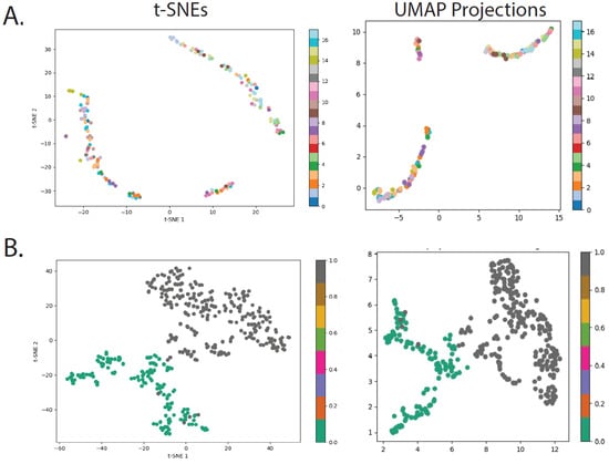
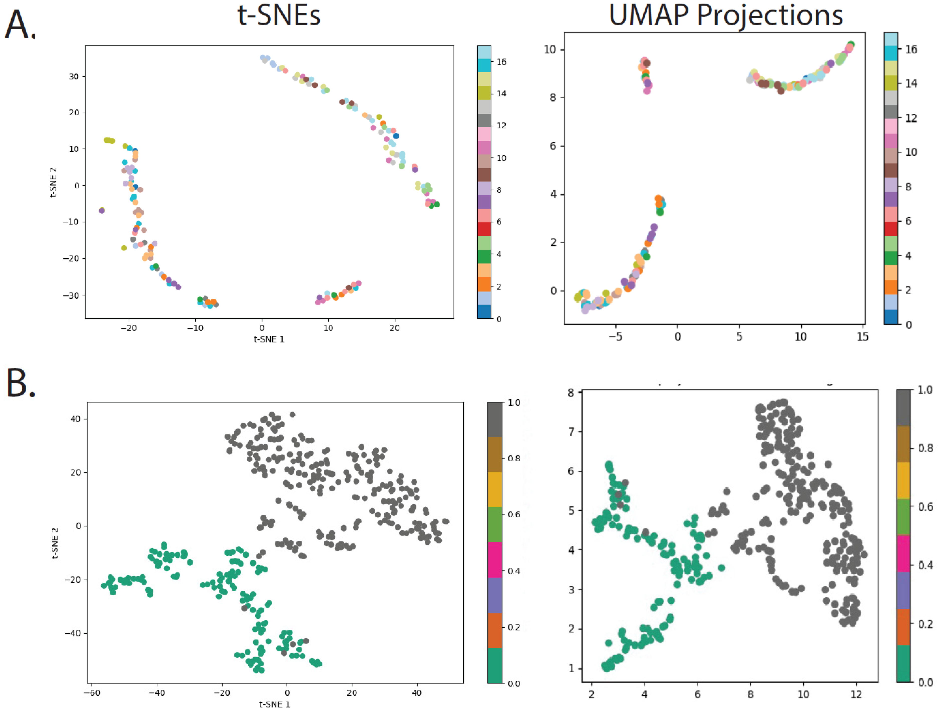
The highest ARI obtained using geometric morphometric methods was 0.068, obtained using either the 100 distances and the hierarchical approach or all traits and the k-means clustering approach for the Barrington population (Table 1). The highest ARI for the Thomson population was 0.055, while the highest for the combined populations was 0.065 (Table 1). Thus, none of the traits and clustering method combinations using geometric morphometrics did much better than randomly sorting clutch-mate groups. The neural network approach was better, with a maximum ARI of 0.266 obtained using the convolutional autoencoder and hierarchical clustering (Figure 3 and Figure S2, Table 2). The Wild-ID software clustering of the Barrington population by clutch had an ARI of −0.001 for hierarchical clustering and 0.008 +/− 0.005 for k-means. The Thomson population ARI was 0.007 for hierarchical clustering and 0.022 +/− 0.005 for k-means clustering, and the combined population ARI was 0.010 and 0.007 +/− 0.002.
Table 1.
Adjusted Rand indices (ARIs) with +/− standard deviation for the k-means clustering of each combination of clustering method and pattern trait to measure the effectiveness of geometric morphometric methods for identifying clutches based on plastron patterns of Chrysemys picta from two different populations, analyzed separately and together. Adjusted Rand Indices fall between −1 and 1, with 0 being random clustering and 1 being perfectly accurate clustering. Bold font denotes the highest performing cluster and trait for each subset.
Figure 3.
Visualizations of the convolutional autoencoder embeddings for (A) clutch-mate clusters in Barrington and (B) populations, using t-SNE and UMAP projections. In (A), different colors denote different clutches, with an ARI of 0.266. In (B), green points represent the Barrington population while grey represents Thomson, with an ARI of 0.858.
Table 2.
Adjusted Rand Indices (ARIs) with +/− standard deviation for the k-means clustering of each combination of clustering method and model method to measure the effectiveness of neural network models for identifying clutches based on plastron patterns of Chrysemys picta. Adjusted Rand Indices fall between −1 and 1, with 0 being random clustering and 1 being perfectly accurate clustering. Bold font denotes the best performing cluster and model for each population of turtles, with the highest ARI for each population obtained using geometric morphometric methods (Table 1) in parentheses to facilitate comparison.
3.2. Population Classifications
Using geometric morphometrics, the most effective clustering by population group used the percent area of the plastron occupied by the pattern, with the K-means approach, obtaining an ARI of 0.792 (Table 3). Using hierarchical clustering, the highest ARI was 0.773 and also used the percent area measurement. The neural network approach was able to obtain an ARI of 0.858 using the convolutional autoencoder and hierarchical clustering (Table 4), meaning individuals were well classified into populations (Figure 3 and Figure S3). The Wild-ID software clustering by population had an ARI of −0.004 using hierarchical clustering and 0.030 +/− 0.04 using k-means clustering.
Table 3.
Adjusted Rand Indices (ARIs) with +/− standard deviation for the k-means clustering of each combination of clustering method and pattern trait to measure effectiveness of geometric morphometric methods for identifying source populations based on plastron patterns of Chrysemys picta. ARIs fall between −1 and 1, with 0 being random clustering and 1 being perfectly accurate clustering. The bold font denotes the highest performing trait.
Table 4.
Adjusted Rand Indices (ARIs) with +/− standard deviation for the k-means clustering of each combination of clustering method and pattern trait to measure the effectiveness of neural network methods for identifying source populations based on plastron patterns of Chrysemys picta. ARIs fall between −1 and 1, with 0 being random clustering and 1 being perfectly accurate clustering. The bold font denotes the best performing method. Feature spaces for these models are visualized in Figure S2.
4. Discussion
In this case study, we demonstrate that both geometric morphometric methods and the convolutional neural network produce clustering that closely corresponded with the source populations (ARIs = 0.792–0.858) but not with clutch membership (ARIs < 0.266). In both cases, features extracted from CNN architectures outperformed the traditional pattern extraction and geometric morphometric approach.
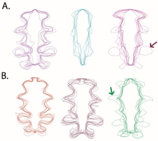
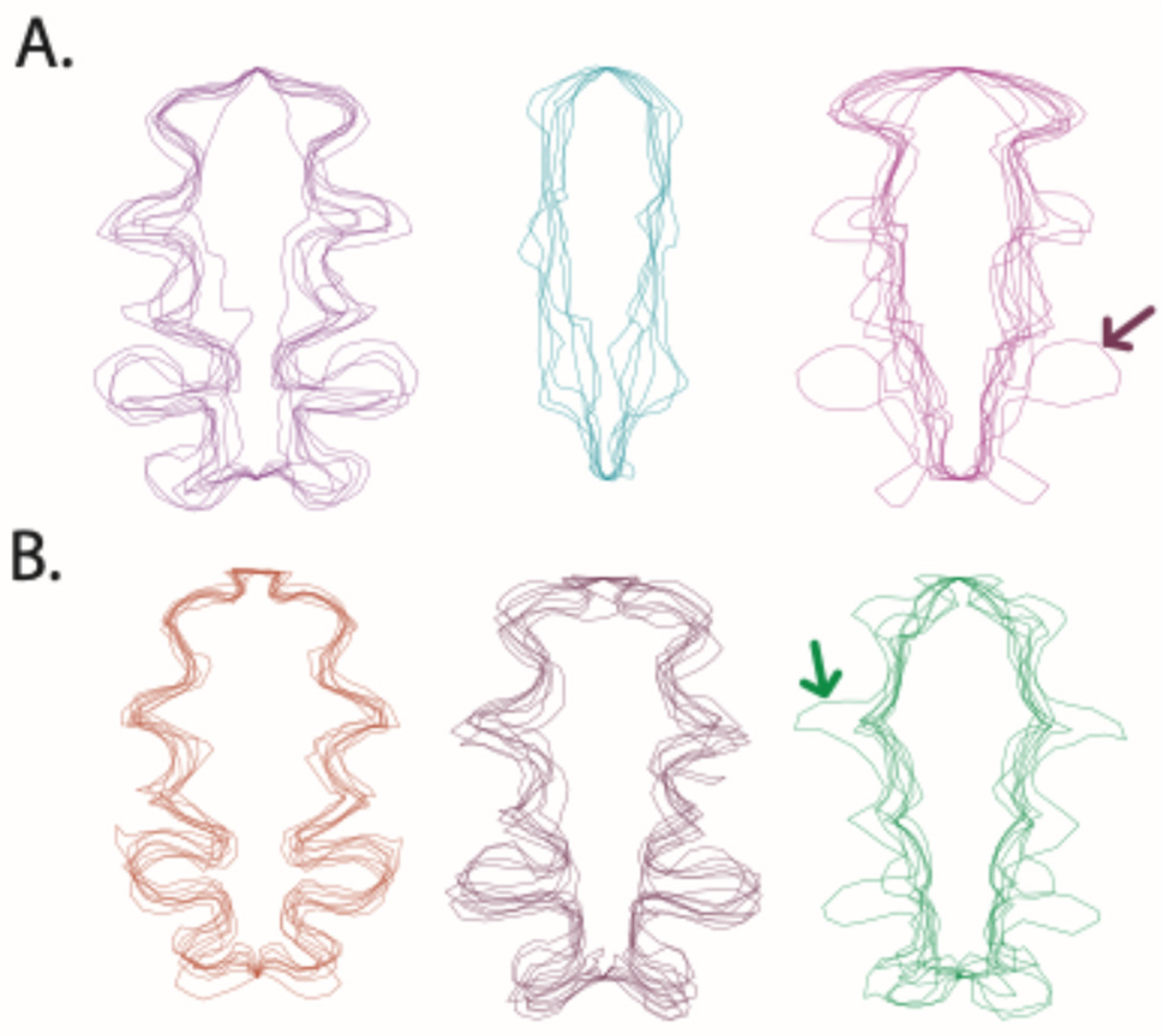
The differences in plastron patterns between populations are not distinguishable to the human eye; however, clutch-mates do often appear to have similar patterns. This species is complicated by multiple paternity, which results in a range of full and half siblings in a clutch. In a previous study using the Thomson population, over 30% of the sampled clutches contained incidences of multiple paternity [18] and thus it is fairly common. Visually, the patterns within a clutch are often only moderately variable, with the occasional outlier that may represent alternative paternity (Figure 4), though this has not been tested. These may make it much more difficult for either method to reliably classify clutch-mates in painted turtles, but does not discount the potential applicability of the CNN approach to other species. We did find more success in grouping by clutch in the small, isolated population (Barrington: 0.266) than in the much larger population (Thomson: 0.029), and intermediate success when the populations were combined (0.124). This suggests that more training data from more populations could improve the efficacy of grouping by relatedness, though it is unknown if the Barrington population had a different level of multiple paternity. Clutch sizes did not differ between the two populations, ranging from 6 to 13 in both. Because the CNNs were trained using images from a different population than those used in the clustering analyses, it is possible that the features learned during training emphasized visual variation that is informative at the population level rather than more subtle variation associated with relatedness. However, this feature extraction did not involve labeling or clustering. Thus, training on a different population would not be expected to directly bias the networks, but the training population may nevertheless have influenced which visual features were represented in the resulting embeddings. Though we converted all images to grayscale to try to remove any differences in lighting between populations, we cannot verify for certain that the CNN architecture only identified biological differences between populations. Training on images from multiple populations could therefore improve the ability of the learned representations to capture variation that is relevant to relatedness, although this remains to be tested. Surprisingly, we identified differences in which traits and even which clustering methods were best between populations, suggesting that there is no single trait measurement that contains enough information for clustering in this species. Thus, when the heredity and/or biological relevance of an organismal pattern is not known, it is especially important to validate it as we did here, before testing on unknown samples.
Figure 4.
(A). The plastron patterns of three representative clutches from the Barrington population and (B). three representative clutches from the Thomson population. The plastron patterns of painted turtles (Chrysemys picta) appear to vary more between clutches than within them (half or full siblings are illustrated in the same color together). This species exhibits multiple paternity and so the individuals with very different plastron patterns may represent individuals with different sires (arrows). Outlines were Procrustes superimposed for all analyses.
The geometric morphometric method requires time-consuming post-processing and the CNN approaches require training data (though they can be from the same or different populations, as was done here). A limitation of either approach is the need to know the number of groups in which to sort the images. This may not be limiting when the average number of offspring is known in a population, or when the number of source populations can be estimated, but could be a consequential limiting factor if those data are not available. Validating how much information can be extracted from a pattern first may allow for unsupervised, undefined clustering in certain species, which would then allow for broader applications. Deep learning generates a “black box”-style classification in which the underlying evidence used to sort images is not identifiable. Thus, researchers should take care not to over-extend the biological implications of any pattern traits they do identify.
Researchers who run long-term wildlife studies are often limited by the time required to match photographs in order to identify individuals. Some software programs exist to facilitate this matching process such as Wild-ID [30], I3S [6], and HotSpotter [34] while many others are restricted to particular species (e.g., StripeSpotter, LemurFaceID) [35,36]. The resulting data can only relate one individual photo to another photo of the presumably same individual and do not allow for any quantification of pattern or estimation of other related variables. As we verified here, the similarity scores calculated by programs like Wild-ID are not adequate substitutes for feature extraction using more direct methods like neural networks or geometric morphometric analyses. Here, we tested CNN architectures with researchers who already perform image processing to identify individuals in mind. They are likely to already have large numbers of labeled photographs for use in software like Wild-ID, so should have training data readily available, and running CNNs can allow them to extract data and address questions about individual groupings that existing methods cannot. Note that we intentionally used standard and well-known neural network architectures and approaches because our intent was to show their applicability to this class of problem. For similar reasons, we did not attempt optimizations like ablation studies because our goal is to provide tools and an environment that other biological researchers could use, rather than optimizing the approach for one problem. Collaborations and clear communication between disciplines is necessary for the future of analyzing animal patterns and other biometrics [5]. Publicly available datasets, like WildlifeDatasets [37], are making this type of approach more feasible for non-computer scientists. Thus, providing tools and validating use cases will be increasingly important as the technology becomes more accessible.
In hindsight, it is unsurprising that the autoencoder-based feature extraction approach outperformed the segmentation-based approach. The convolutional autoencoder had available to it every aspect of the grayscale image from which to extract features and compress information, while the segmentation models were only able to do so in the context of achieving a good segmentation. We expect that this will hold true in other areas of biology, and a researcher that wants to use these tools should start with a convolutional autoencoder approach.
Potential future applications of this CNN approach to other species include returning trafficked organisms to their original population, or identifying the population of origin to tighten anti-poaching efforts. These applications would require significant validation specific to each species before use due to the fine-detail required and the variation in pattern information across or within species. With appropriate validation and testing, researchers who run long-term studies may be able to use this method to identify the parent or parents of individuals of unknown birth when most family groups can be identified, or to make other inferences about population genetics [38]. CNNs could also be applied to identify cryptic species within species complexes (i.e., two or more species that look similar to the human eye, or cannot be distinguished without invasive methods), or to sex species with subtle or undetectable sexual dimorphism [39]. The grouping power of this method is constrained only by the types of training data available, and the information contained within any given animal pattern.
5. Conclusions
We found that the information extracted from painted turtle plastrons patterns by four neural network architectures outperformed the data gathered with traditional geometric morphometric methods in producing clustering that closely matched source populations. Neither approach was able to cluster patterns that matched clutch-mates (half or full siblings). Both approaches significantly outperformed the clustering obtained using similarity scores calculated by Wild-ID for both types of biological groups. Here, we demonstrate that neural network architectures can be powerful tools for extracting animal pattern information to then be clustered into biologically relevant groups, and that they can outperform existing approaches.
Supplementary Materials
The following supporting information can be downloaded at https://www.mdpi.com/article/10.3390/mca31050230/s1. Data S1: X and y coordinates and percent areas of the plastron patterns of Chrysemys picta; Data S2: Similarity scores calculated by WildID for each pair of Chrysemys picta photos; ImagesFiles: A zipped file containing the photos used for the training dataset; Figure S1: Visualizations of the embeddings for clutch-mate (half or full siblings) clusters from Barrington using t-SNE and UMAP projections. Figure S2: Visualizations of the embeddings for population clusters using t-SNE and UMAP projections. Table S1: Adjusted Mutual Information (AMIs) with +/− standard deviation for the k-means clustering of each combination of clustering method and pattern trait to measure the effectiveness of geometric morphometric methods for identifying clutches based on plastron patterns of Chrysemys picta from two different populations, analyzed separately and together. Table S2: Adjusted Mutual Information (AMIs) with +/− standard deviation for the k-means clustering of each combination of clustering method and model method to measure effectiveness of neural network models for identifying clutches based on plastron patterns of Chrysemys picta. Table S3: Adjusted mutual information (AMIs) with +/− standard deviation for the k-means clustering of each combination of clustering method and pattern trait to measure effectiveness of geometric morphometric methods for identifying source populations based on plastron patterns of Chrysemys picta. Table S4: Adjusted Mutual Information (AMIs) with +/− standard deviation for the k-means clustering of each combination of clustering method and pattern trait to measure the effectiveness of neural network methods for identifying source populations based on plastron patterns of Chrysemys picta. Table S5: Adjusted Mutual Information (AMIs) with +/− standard deviation for the k-means clustering of each combination of clustering method and group to measure the effectiveness of WildID to identify clutches and source populations based on plastron patterns of Chrysemys picta.
Author Contributions
Conceptualization, B.A.R., R.R. and N.K.; methodology, R.R., N.K., A.H. and D.T.; software, R.R., N.K., A.H. and D.T.; formal analysis, A.I., N.K. and A.H.; investigation, A.I., N.K. and A.H.; resources, B.A.R., R.R., N.K. and M.A.C.; data curation, B.A.R., N.K. and M.A.C.; writing—original draft preparation, A.I. and B.A.R.; writing—review and editing, B.A.R., A.I., N.K., D.T., A.H., M.A.C. and R.R.; visualization, N.K.; supervision, B.A.R. and R.R.; project administration, B.A.R. and R.R.; funding acquisition, B.A.R., R.R. and N.K. All authors have read and agreed to the published version of the manuscript.
Funding
Funding was provided by the Student Center for Science Engagement, a National Science Foundation PRIMES grant to NK (#2331502), and a National Science Foundation BRC-BIO grant to BAR (#2233233).
Data Availability Statement
The data obtained using the geometric morphometric approach (i.e., x and y coordinates; Data S1) and the Wild-ID similarity scores (Data S2) are available as Supplementary Material, along with the R code used to analyze them and produce the results. The neural network architecture and code are available on GitHub (DOI: 10.5281/zenodo.22309471). The training images are available as Supplementary Material also (ImageFiles).
Acknowledgments
The authors would like to thank the Thomson field crews of 2023 and 2024, including Janzen Lab personnel from Michigan State University and Reinke Lab personnel from Northeastern Illinois University, the Fall 2021 NEIU BIO 324 Local Fauna class, and the Krause family, all of whom assisted with collecting the eggs and photographing hatchlings for this study.
Conflicts of Interest
Authors Beth A. Reinke and Robert Reinke are related, and both are on the board of Intelligent Information Corp., which employs Robert Reinke, Andrew Hanigan, and Dylan Todd. However, this project was funded entirely by the National Science Foundation which subcontracted Intelligent Information Corp. Therefore the funders had no role in the design, interpretation, writing, etc. of the study. The remaining authors declare that the research was conducted in the absence of any commercial or financial relationships that could be construed as a potential conflict of interest
Abbreviations
The following abbreviations are used in this manuscript:
| ANN | Artificial neural network |
| ARI | Adjusted Rand indices |
| CNN | Convolutional neural network |
| DFS | Deep feature space |
| DNN | Deep neural network |
References
- Lee, D.E.; Cavener, D.R.; Bond, M.L. Seeing Spots: Quantifying Mother-Offspring Similarity and Assessing Fitness Consequences of Coat Pattern Traits in a Wild Population of Giraffes (Giraffa camelopardalis). PeerJ 2018, 6, e5690. [Google Scholar] [CrossRef] [Scilit]
- Amelon, S.K.; Hooper, S.E.; Womack, K.M. Bat Wing Biometrics: Using Collagen–Elastin Bundles in Bat Wings as a Unique Individual Identifier. J. Mammal. 2017, 98, 744–751. [Google Scholar] [CrossRef] [Scilit]
- Duffy, J.; Stragliotto, T.; Mella, V.S.A. On the Nose: Validating a Novel, Non-Invasive Method to Identify Individual Koalas Using Unique Nose Patterns. Wildl. Res. 2024, 51, WR24131. [Google Scholar] [CrossRef] [Scilit]
- Battey, C.; Ralph, P.L.; Kern, A.D. Predicting Geographic Location from Genetic Variation with Deep Neural Networks. eLife 2020, 9, e54507. [Google Scholar] [CrossRef] [Scilit]
- Kühl, H.S.; Burghardt, T. Animal Biometrics: Quantifying and Detecting Phenotypic Appearance. Trends Ecol. Evol. 2013, 28, 432–441. [Google Scholar] [CrossRef] [Scilit]
- Hartog, J.D.; Reijns, R. I3S: Interactive Individual Identification System; Reijns Free Software Foundation Inc.: Boston, MC, USA, 2014. [Google Scholar]
- Nazir, S.; Kaleem, M. Advances in Image Acquisition and Processing Technologies Transforming Animal Ecological Studies. Ecol. Inform. 2021, 61, 101212. [Google Scholar] [CrossRef] [Scilit]
- Borowiec, M.L.; Dikow, R.B.; Frandsen, P.B.; McKeeken, A.; Valentini, G.; White, A.E. Deep Learning as a Tool for Ecology and Evolution. Methods Ecol. Evol. 2022, 13, 1640–1660. [Google Scholar] [CrossRef] [Scilit]
- Schneider, S.; Taylor, G.W.; Linquist, S.; Kremer, S.C. Past, Present and Future Approaches Using Computer Vision for Animal Re-Identification from Camera Trap Data. Methods Ecol. Evol. 2019, 10, 461–470. [Google Scholar] [CrossRef] [Scilit]
- Rumelhart, D.E.; Hinton, G.E.; Williams, R.J. Learning Representations by Back-Propagating Errors. Nature 1986, 323, 533–536. [Google Scholar] [CrossRef] [Scilit]
- Rumelhart, D.E.; Durbin, R.; Golden, R.; Chauvin, Y. Backpropagation: The Basic Theory. In Mathematical Perspectives on Neural Networks; Erlbaum: Hillsdale, NJ, USA, 1996; pp. 533–566. [Google Scholar]
- Congdon, J.D.; Nagle, R.D.; Kinney, O.M.; Van Loben Sels, R.C.; Quinter, T.; Tinkle, D.W. Testing Hypotheses of Aging in Long-Lived Painted Turtles (Chrysemys picta). Exp. Gerontol. 2003, 38, 765–772. [Google Scholar] [CrossRef] [Scilit]
- Cooley, C.R.; Smith, S.A.; Geier, C.A.; Puentes, T.G. The Use of Photo-Identification as a Means of Identifying Western Painted Turtles (Chrysemys picta bellii) in Long-Term Demographic Studies. Herpetol. Rev. 2013, 44, 430–432. [Google Scholar]
- Frazer, N.B.; Gibbons, J.W.; Greene, J.L. Growth, Survivorship and Longevity of Painted Turtles Chrysemys picta in a Southwestern Michigan Marsh. Am. Midl. Nat. 1991, 125, 245–258. [Google Scholar] [CrossRef] [Scilit]
- Reinke, B.A.; Miller, D.A.W.; Janzen, F.J. What Have Long-Term Field Studies Taught Us about Population Dynamics? Annu. Rev. Ecol. Evol. Syst. 2019, 50, 261–278. [Google Scholar] [CrossRef] [Scilit]
- Ultsch, G.R.; Ward, G.M.; LeBerte, C.M.; Kuhajda, B.R.; Stewart, E.R. Intergradation and Origins of Subspecies of the Turtle Chrysemys picta: Morphological Comparisons. Can. J. Zool. 2001, 79, 485–498. [Google Scholar] [CrossRef] [Scilit]
- Ernst, C.H.; Lovich, J.E. Turtles of the United States and Canada; JHU Press: Baltimore, MD, USA, 2009. [Google Scholar]
- Pearse, D.; Janzen, F.; Avise, J. Multiple Paternity, Sperm Storage, and Reproductive Success of Female and Male Painted Turtles (Chrysemys picta) in Nature. Behav. Ecol. Sociobiol. 2002, 51, 164–171. [Google Scholar] [CrossRef] [Scilit]
- Pearse, D.E.; Eckerman, C.M.; Janzen, F.J.; Avise, J.C. A Genetic Analogue of “mark-Recapture” Methods for Estimating Population Size: An Approach Based on Molecular Parentage Assessments. Mol. Ecol. 2001, 10, 2711–2718. [Google Scholar] [CrossRef] [Scilit]
- Clark, M.A.; Crowther, C.; Reinke, B.A. Plastral Patterns Serve an Anti-predator Function in Freshwater Turtle Hatchlings. Ecol. Evol. 2026, 16, e73913. [Google Scholar] [CrossRef] [Scilit]
- Janzen, F.J. Climate Change and Temperature-Dependent Sex Determination in Reptiles. Proc. Natl. Acad. Sci. USA 1994, 91, 7487–7490. [Google Scholar] [CrossRef] [Scilit]
- Schneider, C.A.; Rasband, W.S.; Eliceiri, K.W. NIH Image to ImageJ: 25 Years of Image Analysis. Nat. Methods 2012, 9, 671–675. [Google Scholar] [CrossRef] [Scilit]
- Adams, D.C.; Otárola-Castillo, E. Geomorph: An r Package for the Collection and Analysis of Geometric Morphometric Shape Data. Methods Ecol. Evol. 2013, 4, 393–399. [Google Scholar] [CrossRef] [Scilit]
- Core Team R. R: A Language and Environment for Statistical Computing; R Foundation for Statistical Computing: Vienna, Austria, 2024. [Google Scholar]
- Charpentier, M.J.E.; Harté, M.; Poirotte, C.; De Bellefon, J.M.; Laubi, B.; Kappeler, P.M.; Renoult, J.P. Same Father, Same Face: Deep Learning Reveals Selection for Signaling Kinship in a Wild Primate. Sci. Adv. 2020, 6, eaba3274. [Google Scholar] [CrossRef] [Scilit]
- Taigman, Y.; Yang, M.; Ranzato, M.; Wolf, L. DeepFace: Closing the Gap to Human-Level Performance in Face Verification. In Proceedings of the 2014 IEEE Conference on Computer Vision and Pattern Recognition; IEEE: Piscataway, NJ, USA, 2014; pp. 1701–1708. [Google Scholar]
- Pedregosa, F.; Pedregosa, F.; Varoquaux, G.; Varoquaux, G.; Org, N.; Gramfort, A.; Gramfort, A.; Michel, V.; Michel, V.; Fr, L.; et al. Scikit-Learn: Machine Learning in Python. J. Mach. Learn. Res. 2011, 12, 2825–2830. [Google Scholar]
- Van der Maaten, L.; Hinton, G. Visualizing Data Using T-SNE. J. Mach. Learn. Res. 2008, 9, 2579–2605. [Google Scholar]
- Sainburg, T.; McInnes, L.; Gentner, T.Q. Parametric UMAP Embeddings for Representation and Semisupervised Learning. Neural Comput. 2021, 33, 2881–2907. [Google Scholar] [CrossRef] [Scilit]
- Bolger, D.T.; Morrison, T.A.; Vance, B.; Lee, D.; Farid, H. A Computer-Assisted System for Photographic Mark–Recapture Analysis. Methods Ecol. Evol. 2012, 3, 813–822. [Google Scholar] [CrossRef] [Scilit]
- Rand, W.R. Objective Criteria for the Evaluation of Clustering Methods. J. Am. Stat. Assoc. 1971, 66, 846–850. [Google Scholar] [CrossRef] [Scilit]
- Hubert, L.; Arabie, P. Comparing Partitions. J. Classif. 1985, 2, 193–218. [Google Scholar] [CrossRef] [Scilit]
- Chiquet, J.; Rigaill, G.; Sundqvist, M. Aricode: Efficient Computations of Standard Clustering Comparison Measures, version 1.1.0; R Foundation for Statistical Computing: Vienna, Austria, 2018.
- Crall, J.P.; Stewart, C.V.; Berger-Wolf, T.Y.; Rubenstein, D.I.; Sundaresan, S.R. HotSpotter: Patterned Species Instance Recognition. In Proceedings of the 2013 IEEE Workshop on Applications of Computer Vision (WACV); IEEE: Piscataway, NJ, USA, 2013; pp. 230–237. [Google Scholar]
- Lahiri, M.; Tantipathananandh, C.; Warungu, R.; Rubenstein, D.I.; Berger-Wolf, T.Y. Biometric Animal Databases from Field Photographs: Identification of Individual Zebra in the Wild. In Proceedings of the ACM International Conference on Multimedia Retrieval (ICMR 2011); ACM Press: New York, NY, USA, 2011. [Google Scholar]
- Crouse, D.; Jacobs, R.L.; Richardson, Z.; Klum, S.; Jain, A.; Baden, A.L.; Tecot, S.R. LemurFaceID: A Face Recognition System to Facilitate Individual Identification of Lemurs. BMC Zool. 2017, 2, 2. [Google Scholar] [CrossRef] [Scilit]
- Čermák, V.; Picek, L.; Adam, L.; Papafitsoros, K. WildlifeDatasets: An Open-Source Toolkit for Animal Re-Identification. In Proceedings of the 2024 IEEE/CVF Winter Conference on Applications of Computer Vision (WACV); IEEE: Piscataway, NJ, USA, 2024; pp. 5941–5951. [Google Scholar]
- Korfmann, K.; Gaggiotti, O.E.; Fumagalli, M. Deep Learning in Population Genetics. Genome Biol. Evol. 2023, 15, evad008. [Google Scholar] [CrossRef] [Scilit]
- Ortenzi, L.; Costa, C.; Reinke, B.A.; Angelini, C. Using Deep Learning to Distinguish Cryptic Traits in Animal Colour Patterns. J. Zool. 2025, 328, 290–297. [Google Scholar] [CrossRef] [Scilit]

Disclaimer/Publisher’s Note: The statements, opinions and data contained in all publications are solely those of the individual author(s) and contributor(s) and not of MDPI and/or the editor(s). MDPI and/or the editor(s) disclaim responsibility for any injury to people or property resulting from any ideas, methods, instructions or products referred to in the content. |
© 2026 by the authors. Licensee MDPI, Basel, Switzerland. This article is an open access article distributed under the terms and conditions of the Creative Commons Attribution (CC BY) license.