


Abstract
Due to the demands of modern applications, such as forecasting using ordinal continued fraction regression models in economics, the study of structural stability to data perturbations has become an urgent need. While continued fractions demonstrate superior effectiveness over traditional polynomial models due to their inherent structural stability, their sensitivity to coefficient perturbations can lead to accuracy loss under finite-precision machine arithmetic. This paper investigates the stability to perturbations of the coefficients of modified Stieltjes continued fractions (modified S-fractions). We develop a rigorous theoretical framework based on a fundamental recursive formula for the relative error of the nth approximant, expressing error propagation directly in terms of coefficient perturbations. Using this geometric and analytical approach, we establish three distinct uniform stability sets in the complex plane: the half-plane , the angular set under weaker geometric conditions, and the exterior of the disk , which extends verified stability directly to points on and near the imaginary axis. Furthermore, we derive explicit, a priori error bounds for each stability set and prove pointwise stability on a significantly expanded domain, demonstrating that the modified S-fraction remains stable on for any bounded coefficients. These findings establish explicit boundaries for safe computation using standard double-precision arithmetic, providing a mathematical guarantee of algorithmic stability for high-demand contemporary applied models.
Keywords:
continued fraction; stability to perturbations; set of stability to perturbations; relative error; approximant MSC:
30B70; 65G99
1. Introduction
The rapid advancement of computational modeling has established continued fractions as one of the most effective analytical tools for approximating special functions across various fields of science and engineering [1,2]. Traditionally valued for their rapid convergence properties, these mathematical structures have recently found innovative and critical applications in fields driven by empirical data, such as economics [3,4]. For instance, recent developments in forecasting using ordinal continued fraction regression models have demonstrated significantly greater predictive accuracy and stability than traditional polynomial-based models. This operational superiority is largely due to the inherent structural stability of continued fractions to unstable or imperfect real-world inputs.
However, the transition of continued fractions into high-demand contemporary applications exposes them to a critical operational challenge: numerical instability under finite-precision machine arithmetic. In practical implementations, input data are frequently subject to rounding errors, measurement uncertainties, or systemic perturbations. If a computing algorithm lacks sufficient stability, these microscopic perturbations can propagate through successive iterations, leading to a catastrophic loss of significant digits and rendering the model ineffective. Consequently, the demands of modern applied modeling necessitate a rigorous theoretical foundation that can guarantee the structural integrity of specific functional continued fraction classes against complex computational anomalies. To achieve this level of mathematical rigor, it is essential to clearly isolate four interconnected yet distinct concepts: convergence, perturbation stability, numerical stability, and rounding-error analysis.
- Convergence remains a classical, purely analytical property that dictates whether a continued fraction theoretically approaches a precise mathematical limit as the approximant order n approaches infinity under conditions of idealized, infinite precision.
- Conversely, perturbation stability evaluates the inherent capacity of the functional architecture to preserve its output value when its underlying coefficients are permanently altered or corrupted by external data noise, measurement uncertainties, or systemic inputs.
- Numerical stability characterizes the broader operational susceptibility of a specific evaluation algorithm to cumulative mathematical deviations during execution, often dictating the structural choice between forward and backward recurrence mechanisms.
- Finally, rounding-error analysis isolates the specific microscopic precision loss and digit decay triggered by finite-precision machine arithmetic—such as the standard IEEE 754 double-precision unit roundoff constraints—during iterative loops.
By explicitly separating these factors, this paper shifts the analytical focus away from unconstrained convergence metrics toward localized boundary mapping. Among these classes, Stieltjes continued fractions [5] (or S-fractions) occupy a prominent role due to their classic mathematical connections with orthogonal polynomials [6] and the moment problem [7], as well as their wide range of applications in applied problems (see, for example, [8,9,10]).
While their convergence properties are well documented (see [5] or [11] (Theorem 4.58) and [12] (Corollary 5.1), as well as [13,14,15]), existing research often falls short of defining explicit, localized boundaries of stability in the complex plane for their modified variants. Given these practical constraints, this paper theoretically investigates the stability to perturbations of modified S-fractions [2]:
By deriving a new recursive error formula, we map the exact behavioral boundaries of these continued fractions, establishing explicit uniform and pointwise stability sets that ensure computational stability under modern application demands.
1.1. Literature Review
The necessity of evaluating functional continued fractions under nonideal computational conditions has sparked a robust lineage of analytical research. In practical data environments, understanding mere convergence is insufficient; isolating numerical stability, which characterizes the sensitivity of approximant values to rounding and precision loss, is paramount [16]. Early foundations established by Blanch [17] demonstrated that while forward recurrence algorithms (FR-algorithms) are highly susceptible to rapid error accumulation, backward recurrence algorithms (BR-algorithms) exhibit fundamentally superior stability profiles. Building on this operational distinction, Jones and Thron [11,18] pioneered methods to bound the relative error accumulated during backward recurrence by mapping errors directly to the underlying element sets of the continued fractions. These structural error-estimating techniques of continued fractions were subsequently refined [19] and extended to branched continued fraction expansions [20,21,22].
Modern applied modeling, however, places demands on continued fractions that extend beyond standard algorithmic rounding. Since real-world inputs in empirical regression systems are inherently noisy, contemporary research focuses heavily on stability to perturbations—the capacity of a continued fraction to preserve its output value when its functional coefficients are permanently altered by external data errors. For continued fractions with unit partial numerators, these stability zones were mapped by Hladun and Dmytryshyn [23]. Subsequent expansions by these authors established complex stability sets for continued fractions with unified partial denominators, which were successfully applied to map the boundaries of g-fractions [24].
Despite these advancements, traditional S-fractions, despite their deep classical utility in moment problems and orthogonal polynomials, have only recently been evaluated under the lens of perturbation stability. Specifically, Hladun and Dmytryshyn [25] mapped the perturbation stability of S-fractions with complex elements, where the complex variable z acts as a multiplier in the partial numerators () against unit denominators. However, because their error propagation is modeled implicitly as a continued fraction, their framework restricts verified stability to compact, localized interior zones near the origin, producing bounded semi-circular and circular sets.
This paper directly addresses this gap by investigating the modified Stieltjes continued fraction variant, where the variable z forms the mathematical engine of the architecture by acting directly as the partial denominator (). By shifting this underlying functional structure and deriving a fundamental recursive formula for the relative error, we map exact behavioral boundaries that fundamentally expand the geometric scope of perturbation theory. Rather than being confined to bounded regions, our approach establishes vast, unbounded uniform stability sets in the complex plane, including the half-plane the angular set and the exterior of the disk Most notably, while existing classical frameworks encounter mathematical volatility near the imaginary axis, our results extend verified stability directly onto the imaginary axis and its immediate neighborhoods via while guaranteeing pointwise stability across the entire punctured real axis () for any bounded coefficients. This comprehensive mapping provides the precise mathematical assurances required to meet the algorithmic demands of modern applied computational frameworks.
1.2. Computational Experiment and Empirical Stability Stress Test
To evaluate the empirical robustness of the modified S-fraction under conditions that simulate high-demand modern data applications, we conducted a rigorous numerical stress test. In empirical modeling, algorithms must maintain structural integrity when processing noisy inputs or running under finite machine precision. For this experiment, we utilized a modified S-fraction representing the expansion of the square of the ratio of Euler gamma functions [26]:
This specific functional architecture serves as an ideal baseline for testing error propagation because its coefficients grow systematically, mirroring the behavioral complexity found in advanced regression forecasting models.The experiment was structured to observe how micro-level coefficient perturbations—modeled here by standard double-precision rounding errors—accumulate as the complexity of the model increases. Approximants of orders ranging from 1 to 2000 were computed using standard double-precision arithmetic compliant with the IEEE 754 standard (unit roundoff ). To isolate the exact magnitude of accumulated error, these values were compared against highly accurate reference values generated via software-based 128-bit extended precision arithmetic. The relative error was systematically evaluated across a dense grid of test points z in the complex plane, bounded by .
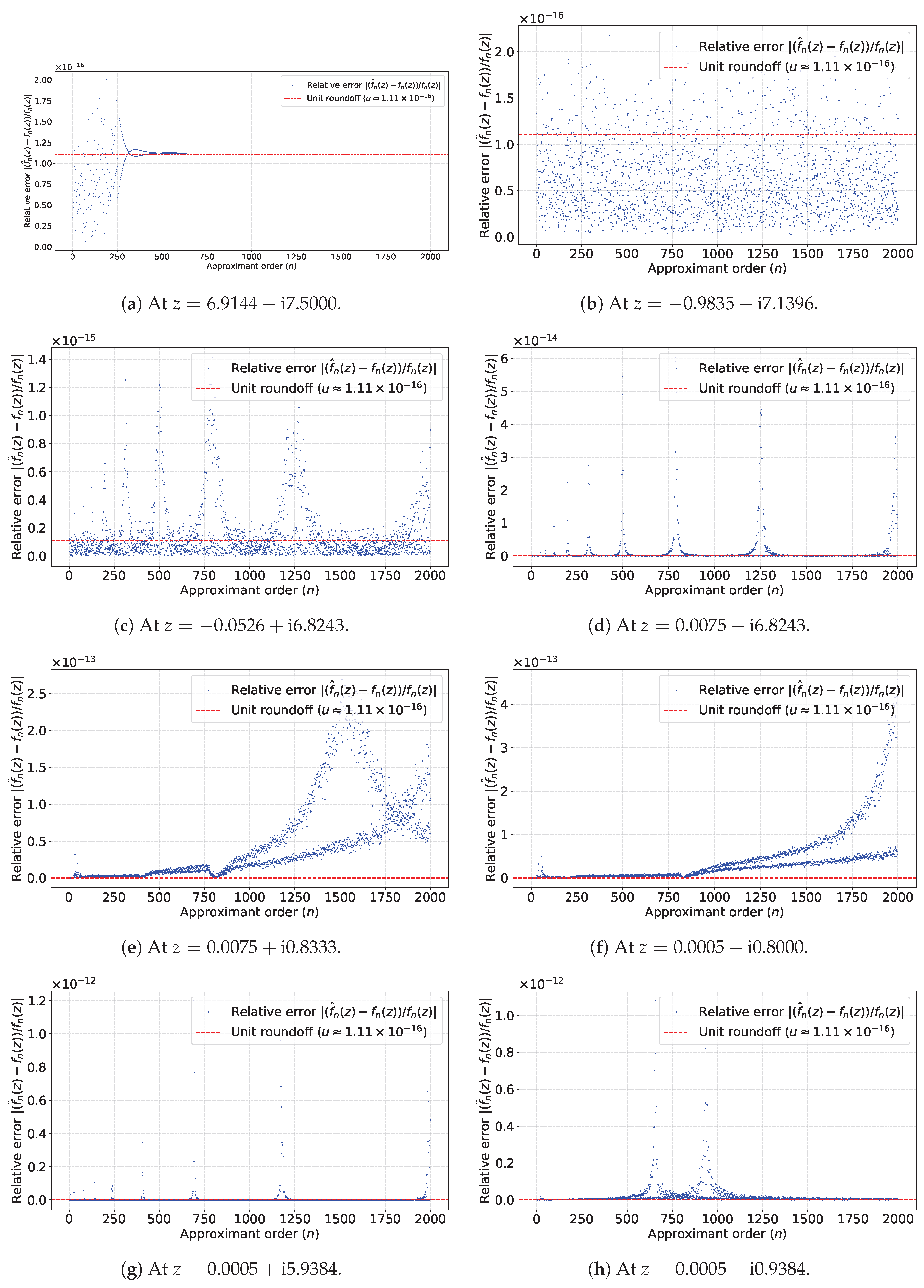
A pointwise analysis of the relative error relative to the approximant order n reveals distinct behavioral zones that dictate the continued fraction’s real-world operational boundaries (see Figure 1a–h). For coordinate points positioned safely away from the origin and the imaginary axis, the modified S-fraction exhibits a remarkable, self-stabilizing structural robustness. In these secure domains, the relative error flatlines at the level of machine precision (≈) and shows absolute resistance to error accumulation, even as the order of the continued fraction scales up to 2000 terms. This profile confirms the continued fraction’s supreme viability for stable execution in standard hardware environments. Conversely, as the test variable z migrates toward the origin, the system encounters a localized volatile zone. Here, the micro-errors accumulate dynamically over successive iterations, driving the relative error up by one to four orders of magnitude ( to ) and resulting in a measurable decay of significant digits.
Figure 1.
Relative errors for continued fraction (2) at selected points z.
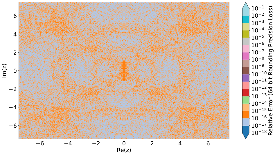
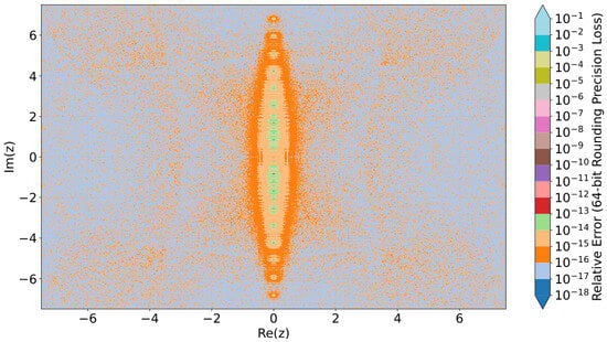
To map this behavior globally, the total distribution of precision loss was rendered into a comprehensive heat map (see Figure 2). The color gradients chart the exact spatial limits of algorithmic robustness under 64-bit rounding constraints. The visual data demonstrate that the vast majority of the complex plane comprises a completely safe computational field where the fraction preserves its structural integrity effortlessly.
Figure 2.
Distribution of relative error for continued fraction (2).
Crucially for modern application design, the zone of accuracy loss does not bleed indefinitely across the complex plane; rather, it is tightly confined to a bounded, symmetrical corridor directly flanking the imaginary axis. This empirical layout proves that numerical instability is not an unmanageable trait of the evaluation algorithm itself but a predictable, spatially bounded phenomenon. For practical software engineering, this implies that standard, high-speed double-precision arithmetic is entirely sufficient for executing these models across major regions of the complex plane, while computationally expensive extended precision frameworks can be strictly rationed for instances where the variable z enters the mathematically verified volatile zone.
In this paper, we investigate this phenomenon theoretically and provide a priori estimates for the relative errors of the approximants. Our main goal is to analyze the stability of the modified S-fraction (1) under perturbations of its coefficients and to establish explicit sets of uniform and pointwise stability in the complex plane. This paper is organized as follows. Section 2 introduces the basic notions and derives a fundamental recursive formula for the relative error of the approximants. Section 3 establishes the sets of uniform stability (Theorems 1–3) and pointwise stability (Corollaries 1, 2, 4) along with explicit error bounds. Section 4 presents the application of the obtained results to the empirical analysis of the stability of the modified S-fraction for the function and to polynomial and continued fraction models for experimental studies and forecasting the dynamics of patent activity in Ukraine. Section 5 contains concluding remarks and outlines directions for further research.
2. Formulas for Relative Rounding Error
Let n be an arbitrary natural number. By perturbing the coefficients , , of the continued fraction (1), we obtain the perturbed modified S-fraction
Denote by
and
the nth approximants of the modified S-fraction (1) and the perturbed modified S-fraction (3), respectively. Assume that for all ,
Definition 1.
We call the modified S-fraction (1) stable to perturbations at a point if for every there exists such that for all , , satisfying the condition
the inequality
holds for all .
Definition 2.
We call the set a set of stability to perturbations of the modified S-fraction (1) if it is stable to perturbations at every point of this set.
Definition 3.
We call the set a set of uniform stability to perturbations of the modified S-fraction (1) if for every there exists such that for all and all , , satisfying the condition
the inequality
holds for all .
Now, denote by
the tails of the nth approximant (4) and the perturbed nth approximant (5), respectively. Assume that , , for all and ,
Next, we establish a formula for the relative error of the approximant (4). For this purpose, we consider the relative errors of the coefficients of the modified S-fraction (3)
the relative error of the nth approximant (5)
and the relative errors of the tails (7)
We also consider the relative errors with respect to the perturbed values
and
Note that the relative errors , and , satisfy the following relations
and
The following lemmas hold.
Lemma 1.
Proof.
Let n be an arbitrary natural number. From formulas (6) and (7), which define the tails and , respectively, the following recurrence relations follow:
and
We will prove that for and the following formula holds
For , we have
Taking into account that
and
we have
Similarly, for , we have
Lemma 2.
Let for all and . Then, for
3. Perturbation Stability Sets
The following theorem holds.
Theorem 1.
Proof.
Let us write the set (15) in the form
where
and
Let n be an arbitrary natural number. By the induction on we prove that
if
For , we have . Since , we get . Suppose that for some k, , the tail . Hence, . Since and , we have
Then
Hence, , .
Since , , we similarly prove that , , if .
Similarly, consider the case where . By induction on k, we prove that for all .
For , we have . Suppose that for some k, , the tail . Then
Since and , we have
Then, for the real part of the kth tail, we obtain:
Hence, . Similarly,
Thus, for any , the tails , for all belong to the same half-plane as the point z.
Let us estimate from above the terms , . From the recurrence relation for the tails of the approximant, we have
Since the variable z and all the tails , , lie in the same half-plane or , their real parts have the same sign. Then
From the last equality, taking into account the estimates and , we have
Since , we get
Multiplying both sides of the inequality by and squaring, we obtain
Denote . From
we have . Consider the function of a real variable
If , then
If , then
Hence,
where
Since the function is continuous and strictly increasing on , on every bounded interval , we have
Hence,
Since the perturbed tails , , have the same properties as the exact tails , , and , , we have
Moreover, from the estimates , , , and the inequalities (13), we obtain
We write the formula for the relative error of the nth approximant (5) in the form
Taking into account that
and the estimates (17)–(19), as well as the fact that from condition (14), for the relative errors , the estimate
follows, from formula (20), we obtain
Since, by the hypothesis of the theorem, , we have . This allows us to relax the estimate for , making it independent of n
Denote the right-hand side of inequality (21) by the function
The function is continuous and strictly increasing on , and
By Definition 1, fix an arbitrary . Using the properties of the function , there exists such that for all perturbations of the coefficients satisfying the condition , the inequality holds. It follows that for all . Hence, the modified S-fraction (1) is stable to perturbations at every point . Since depends only on the constants A and C and does not depend on the choice of the point , by Definition 3, the modified S-fraction (1) is uniformly stable on the set . □
Corollary 1.
Proof.
Let be an arbitrary fixed point in . Then
We set . Then, , where the set is defined by (15). Since the inequality (24) holds, by Theorem 1, the set is a set of uniform stability to perturbations of the modified S-fraction (1). By Theorem 1, for all and all , we have the estimate (16). Setting and taking into account that , we obtain the estimate (23).
By the estimate (23), for an arbitrary , there exists such that the condition , , implies the inequality for all . Hence, the conditions of Definition 1 are satisfied, i.e., the modified S-fraction (1) is stable to perturbations at the point . Finally, since the point is arbitrary, the set is a set of pointwise stability to perturbations of the modified S-fraction (1). □
Next, we prove the following result.
Theorem 2.
Proof.
We split the set according to the sign of the real part
where
and
Let us prove that if , then for all .
For , we have . Suppose that for some . Let us prove . From the recurrence relation , we have
and
Since and , we have
Applying the triangle inequality to the formula for and using the inequalities and , we have
It follows that .
In the case , the reasoning is analogous. Since , we have , , for all .
Hence, for all and
Moreover, if , then from the condition , it follows that
Hence,
Now, let us estimate the terms , . Since the real parts , , have the same sign, we have
Since , we have , and
Taking into account that , we get
Since , multiplying the last inequality by , we obtain
Next, since and , we have
where
We have the same estimate for the perturbed terms namely,
Since the function is strictly increasing on and the coefficients , , , satisfy condition (13), we have
where the condition ensures that the inequality holds. Moreover, taking into account condition (13) and the inequalities (27), we obtain the estimates (19).
Taking into account the estimates (28), (19), from formula (11), we get
Since , we have
The function is continuous, strictly increasing, and
For a fixed , there exists , depending only on the parameters , A, C, such that for , we have . From (29), we obtain
Hence, the modified S-fraction (1) is stable at every point of . □
Remark 1.
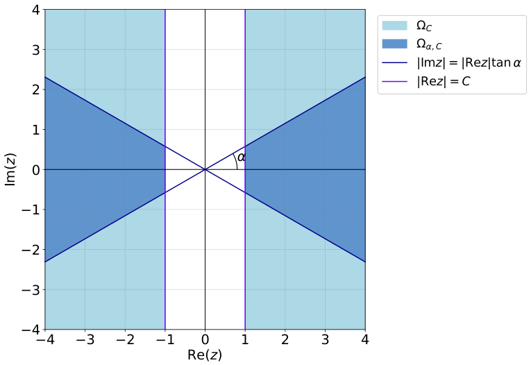
The set is the intersection of the half-plane
with the angular set
The set is the intersection of the half-plane
with the angular set
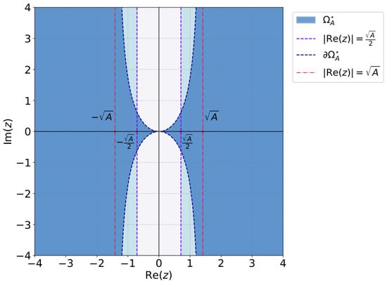
(see Figure 3). The smaller the angle α, the weaker the condition on the constant C that bounds the set . For , the set degenerates into two rays
on the real axis, i.e., the modified S-fraction is uniformly stable to perturbations on the set for arbitrary bounded coefficients.
Figure 3.
Sets of uniform stability to perturbations of modified S-fraction (1).
Remark 2.
Comparing Theorem 1 and Theorem 2, we note that for any and , and as , we have . Since
the lower bound for C in Theorem 2 is smaller than in Theorem 1, and as , it tends to zero (). For , the lower bound in Theorem 2 is greater than in Theorem 1.
Corollary 2.
Proof.
Let be an arbitrary fixed point in . We set
Since , we have , where the set is defined by (25). By the definition of the set (30)
Since condition (33) coincides with the condition of Theorem 2, the set is a set of uniform stability to perturbations of the modified S-fraction (1), and for all and , the estimate (26) holds for the relative error of the approximant. Taking into account (32), the estimate (26) takes the form (31).
Remark 3.
The boundary
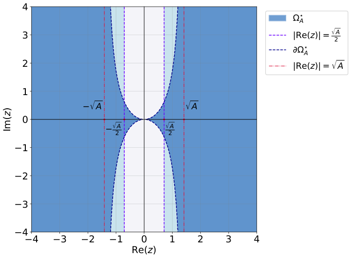
of the domain is a curve symmetric with respect to the coordinate axes, with two vertical asymptotes , whereas the boundary of the domain consists of two straight lines On the real axis, . At the same time, as , the boundary asymptotically approaches the lines , i.e., the domain narrows to the exterior of the domain
Hence, is neither a subset nor a superset of (see Figure 4).
Figure 4.
Set of stability to perturbations of modified S-fraction (1).
The relation between the set of pointwise stability and the sets of uniform stability is described by
i.e., is the union of all sets of uniform stability of the form (25) satisfying the condition of Theorem 2. Moreover, every point belongs to the boundary of the angular set of uniform stability constructed using the parameters (32).
For , condition (33) holds for any . Hence, we obtain the following corollary.
Corollary 3.
The modified S-fraction (1) is stable to perturbations on the set for arbitrary bounded coefficients ,
Theorem 3.
Proof.
Let
where r is defined according to (36). Note that r is the larger root of the equation , so whence .
Let n be an arbitrary natural number. By the induction on k, we prove that for all and .
For , we have
so . Suppose for some . Then, for
i.e., . Since , we similarly prove that for all .
Now, taking into account the estimates , , , and the inequalities (13), we will estimate the terms , , . For an arbitrary , we have
if and
if Hence,
Moreover, from and and the inequalities (13), we have
Taking into account the estimates (37), (38), and the estimate , from formula (20), we obtain (35).
Since , we have . Hence, . Then
The function is continuous, strictly increasing, and
Since does not depend on the point , for an arbitrary , there exists such that for , we have for all and . Hence, by Definition 3, the set is a set of uniform stability to perturbations of the S-fraction (1). □
Remark 4.
It is important to emphasize that the geometric domains , , and established in Theorems 1–3 constitute sufficient conditions for uniform perturbation stability, rather than exact necessary-and-sufficient boundaries. Because these regions are derived using the uniform bounding parameter to guarantee algorithmic robustness for any arbitrary sequence of bounded coefficients, they represent a conservative inner envelope of stability. Consequently, while individual modified S-fractions with highly regular or rapidly decaying coefficient sequences may exhibit empirical stability beyond these thresholds, the boundaries defined herein provide an absolute, structurally guaranteed safety zone against unbounded rounding-error amplification under worst-case parameter configurations.
Remark 5.
Theorem 3 establishes uniform stability on the exterior of the disk , which contains points of the imaginary axis and its neighborhoods, under the condition . This distinguishes it from Theorems 1 and 2, where the sets of uniform stability are isolated from the imaginary axis by the conditions and , respectively. However, the condition of Theorem 3 is stronger than the condition of Theorem 1 for the same value of the parameter ()—the minimal admissible radius in Theorem 3 is four times larger than the minimal value in Theorem 1. Thus, Theorem 3 requires greater distance from the origin but ensures stability to perturbations on the imaginary axis.
Corollary 4.
Proof.
Let an arbitrary fixed point in . Then, . We set . Then, , and since , by Theorem 3, the set is a set of uniform stability to perturbations. From the estimate (35) with , the conditions of Definition 1 are satisfied. By the arbitrariness of , the set is a set of pointwise stability to perturbations of the modified S-fraction (1). □
4. Numerical Experiments
To bridge the theoretical perturbation bounds established in Section 3 with practical computing environments, we consider the constraints imposed by machine precision. When evaluating a modified S-fraction on a digital processor, the continuous coefficients are mapped to a finite-precision representation . Under the standard IEEE 754 double-precision floating-point format, this representation introduces a deterministic roundoff error governed by the unit roundoff (machine epsilon) , such that the relative coefficient error satisfies
Our framework proves that uniform algorithmic stability is preserved provided that the coefficient perturbations do not exceed the structural threshold . Consequently, within the specified stability sets (, , and ) where the geometric criteria dictate that , standard double-precision arithmetic is mathematically sufficient to prevent exponential error amplification. In these sets, the intrinsic rounding noise of the machine is safely bounded within the stability sets, guaranteeing that the backward recurrence algorithm remains robust against catastrophic precision loss.
4.1. Empirical Stability Analysis of the Modified S-Fraction for
To verify the empirical stability of the modified S-fraction satisfying the conditions of the theoretical results, let us consider the expansion of the function into a continued fraction (see, for example, [2])
Unlike the expansion of the square of the ratio of Euler gamma functions considered in Section 1.2, where the partial numerators tend to infinity, in this expansion, the coefficients are given by the formula
and are bounded, converging to the limit as .
To study the behavior of the errors of the approximants , , standard double-precision arithmetic compliant with the IEEE 754 standard (where the unit roundoff is ) was used. The obtained values were compared against high-precision reference values , computed using 128-bit extended precision arithmetic. The relative error was investigated on a grid of points in the complex plane bounded by , .
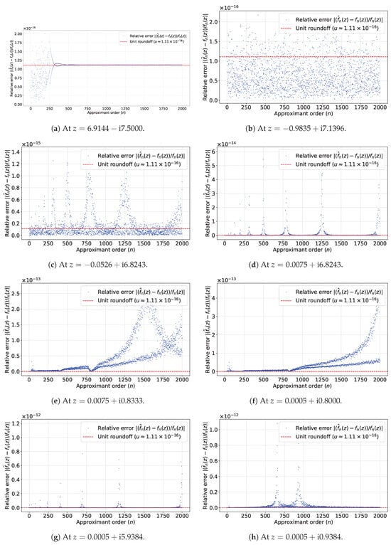
Pointwise analysis of the relative error behavior depending on the approximant order n demonstrates stability of the expansion (see, Figure 5a–h). In most points of the complex plane, the relative error remains at the machine epsilon level (≈), demonstrating resistance to the accumulation of rounding errors even as the approximant order increases up to 2000. At the same time, a loss of accuracy of two orders of magnitude is observed near the imaginary axis and the origin; however, it is significantly smaller compared to the expansion with unbounded partial numerators.
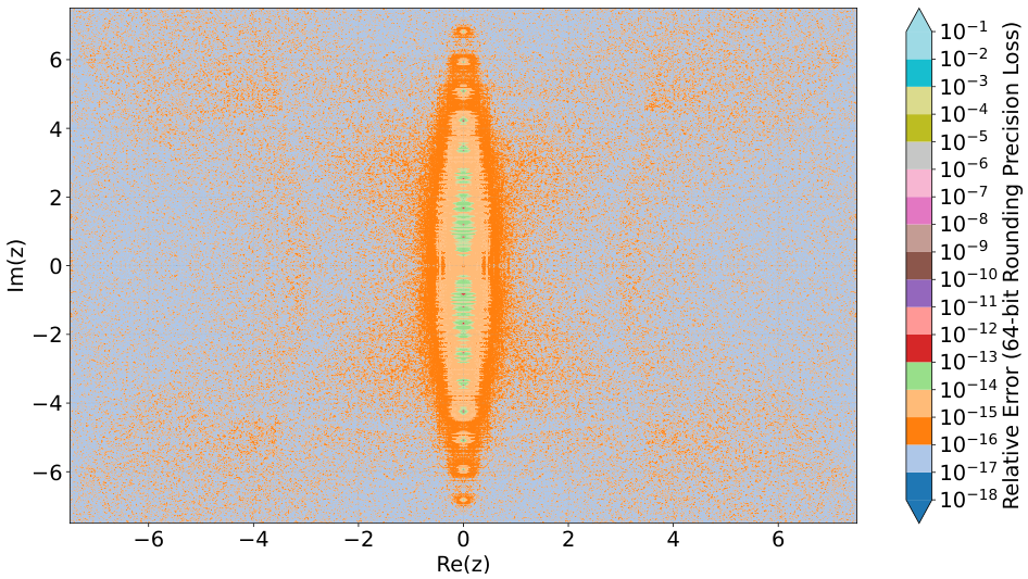
Analyzing Figure 6, we see that high computational precision (at the machine epsilon level ≈) is preserved not only in the domain
but also within it, with the exception of a small neighborhood of the origin along the imaginary axis. This illustrates that the theoretical conditions obtained in this paper are sufficient, but, in practice, the stability domain is wider. The region of accuracy loss (where the error increases up to ) is symmetrically concentrated along the imaginary axis and localized near the origin. Unlike continued fractions with unbounded numerators, where the effects of significant error accumulation spread more widely, the boundedness of the coefficients ensures the damping of errors over a broader region. The fact that practical precision is preserved even in those areas of the complex plane where theoretical results do not yield stability guarantees confirms the high reliability of the modified S-fraction, as well as the current lack of methods for expanding stability domains and the prospects for further research.
Figure 5.
Relative errors for continued fraction (41) at selected points z.
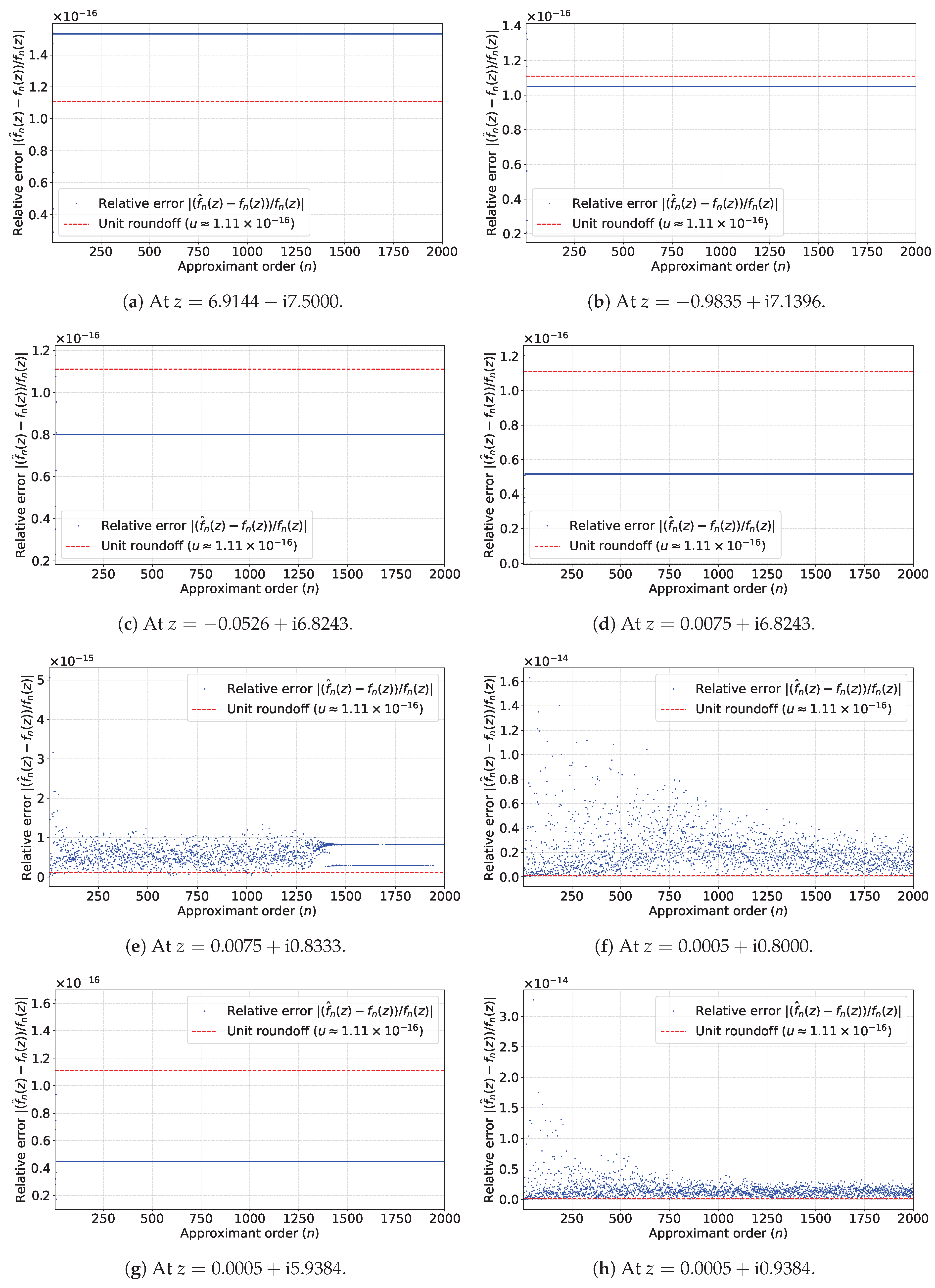
Figure 6.
Distribution of relative error for continued fraction (41).
4.2. Experimental Studies and Forecasting of Patent Activity Dynamics
To verify the effectiveness and predictive properties of the developed mathematical models, the time series of annual patent application volumes in Ukraine for the period of 2016–2025 was chosen as the baseline experimental dataset [27].
To simplify computational procedures and eliminate the scaling effect, the independent variable x (calendar years) was normalized as , then corresponds to the period of 2016–2025. The values of the function y represent the actual number of registered patents. The experimental data are presented in Table 1.
Table 1.
Baseline time series of patent activity.
Within the experiment, four classes of approximation models were constructed and compared:
- Linear model (1st order):
- Quadratic model (2nd order):
- Cubic model (3rd order):
- Continued fraction model (4th order):
The obtained parameter estimation and regression models’ accuracies are as follows:
- Linear model:
- Quadratic model:
- Cubic model:
- Continued fraction model:
Table 2 presents the residual values (residuals), which are defined as the difference between the actual and calculated value .
Table 2.
Residual values table.
The main criterion for selecting the best model is not only the accuracy of describing past data () but also the predictive efficiency during extrapolation over long time periods. Table 3 shows the results of forecast calculations for the period up to 2035.
Table 3.
Comparative table of patent activity forecasts (2026–2035).
The Compound Annual Growth Rate according to the continued fraction model for the period of 2016–2035 is 2.76%.
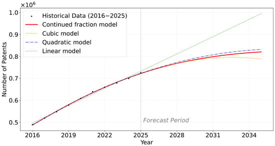
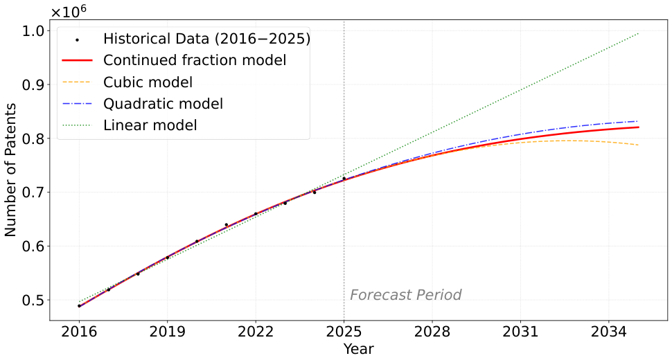
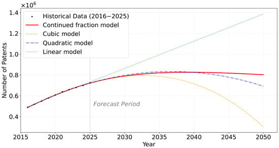
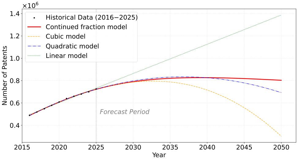
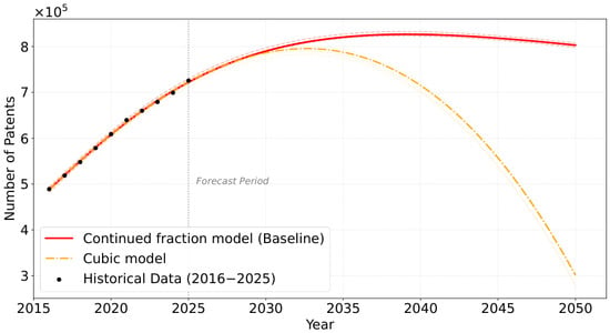
Although the cubic polynomial demonstrates a high value of , the experiment expanding the forecast interval to 2050 clearly demonstrates the overfitting effect and the manifestation of Runge’s phenomenon. On a short interval up to 2035 (see Figure 7), the cubic curve behaves adequately, but over a long distance (, after 2035), it loses adequacy and demonstrates a sharp drop (the forecasted value collapses to 301,102 patents in 2050), which contradicts the economic logic of market development (see Figure 8).
Figure 7.
Patent activity forecasting up to 2035.
Figure 8.
Patent activity forecasting up to 2050.
The linear model predicts unrealistic infinite growth (up to 1.38 million patents in 2050), contrary to the market saturation effect. The quadratic model behaves more realistically, but in the absence of asymptotic constraints, it also demonstrates a decline in the second half of the forecast period. The nonlinear continued fraction model provides the best balance. On the historical interval, it ensures the highest accuracy (), while on the long-term horizon (up to 2050), it implements the property of asymptotic saturation. The curve smoothly reaches a plateau (stabilizing at the level of ∼803–826 thousand patents), which correctly reproduces the processes of market saturation and the exhaustion of growth potential.
Thus, the continued fraction model is an optimal analytical tool that combines high-quality approximation of past data with adequate behavior during long-term extrapolation.
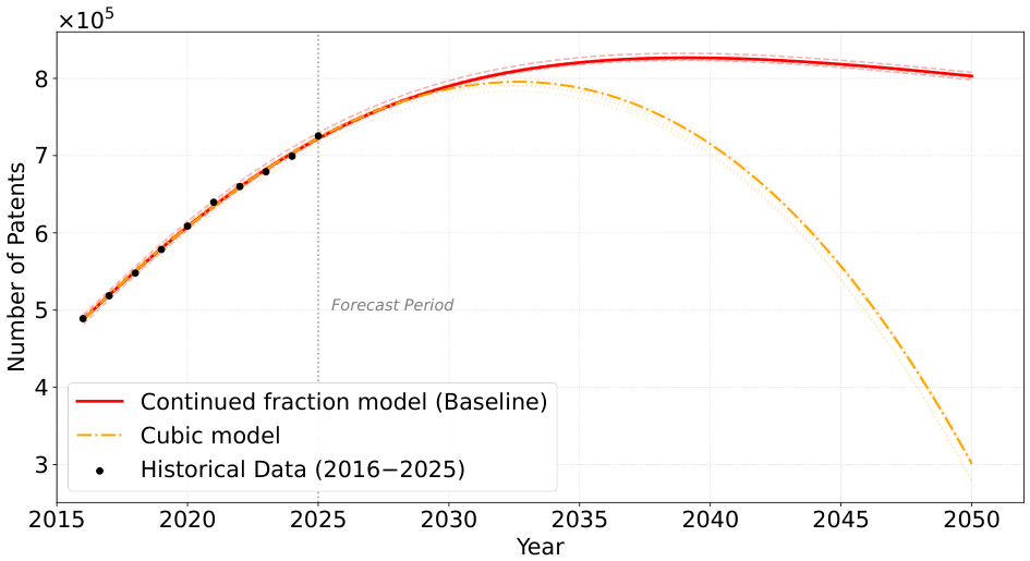
To evaluate the reliability and stability of the constructed models, a coefficient perturbation experiment was conducted. The essence of the experiment consists of randomly perturbing all coefficients of both the cubic model and the continued fraction model within . For each of the five independent perturbation scenarios, we analyzed the quality of approximation on the historical interval (the statistic) and the stability of the forecasted trends over the medium-term (up to 2035) and long-term (up to 2050) intervals. The results of this experiment are presented in Table 4 and Figure 9.
Table 4.
Results of the model parameter perturbation experiment and their impact on the metric and forecasting.
Figure 9.
Stability analysis to coefficient perturbations .
An analysis of the obtained data indicates significant differences in the behavior of the models under perturbation. The cubic model demonstrates noticeable sensitivity to its coefficients; in the worst-case scenario (Test 4), the coefficient of determination drops to . In contrast, the continued fraction model maintains high data-fitting quality, keeping above , which confirms its lower sensitivity to perturbations. Under the influence of random coefficient perturbations, the forecasted trends of the cubic model exhibit marked fluctuations, forming a range from 774,276 to 792,501 patents (an oscillation amplitude exceeding 18,000 units). Conversely, under perturbations, the continued fraction model provides a more reliable forecast (817,817–826,909), minimizing strategic planning risks in the medium term (up to 2035). When performing long-term forecasting for 2050, perturbations of the cubic model parameters push the forecast down even further into an unrealistic range of 278,571–305,210 patents. On the other hand, the continued fraction model successfully reproduces the market saturation effect (plateau effect), providing a stable forecast for 2050 within the range of 798,292–807,836 patents.
Thus, the experimental results illustrate the perturbation stability property of the continued fraction model, making it a reliable tool for long-term forecasting.
Calculations were performed using Maple software 2022.2 for Windows.
5. Conclusions
This paper investigates the stability of modified Stieltjes continued fractions against coefficient perturbations, a study directly driven by the rigorous demands of modern applied modeling. As functional continued fractions increasingly displace traditional polynomials in high-stakes fields like economic regression forecasting, establishing mathematical guarantees of their structural stability has become critical. By shifting the analytical focus from abstract convergence to explicit numerical stability, this study bridges a vital gap between theoretical continued fraction analysis and stable algorithmic implementation.
The cornerstone of our approach is the development of recursive error formulas (Lemmas 1 and 2), which explicitly map how localized coefficient perturbations propagate into the relative error of the nth approximant. These formulas allowed us to establish clear, geometrically defined zones of computation in the complex plane:
- The half-plane : proved to be a set of uniform stability under the condition .
- The angular set : established as a subset of that guarantees uniform stability under a weaker geometric constraint () when .
- The exterior disk : extended uniform stability directly onto the imaginary axis and its immediate neighborhoods, provided that the distance from the origin satisfies .
Crucially, our pointwise analysis successfully expands the verified domain of computational safety, culminating in the proof that modified S-fractions maintain absolute stability across the entire real axis excluding the origin () for any bounded coefficients. For practical software engineering and applied data science, these results provide a concrete blueprint for error management. The explicit a priori error bounds derived for each stability set eliminate algorithmic guesswork. They definitively indicate where standard double-precision arithmetic (IEEE 754) is entirely sufficient to maintain structural integrity and precisely isolate the volatile zones near the origin where extended precision arithmetic is mandatory.
While this study establishes an authoritative baseline for positive real coefficients, modern empirical data often introduce broader algebraic complexities. Consequently, generalizing this recursive error framework to complex coefficients and directly mapping these stability boundaries onto the explicit expansions of active economic forecasting functions represent the priority directions for our further research.
Author Contributions
Conceptualization, R.D.; investigation, V.H.; software, V.H.; writing—original draft, V.H.; writing—review and editing, R.D.; project administration, R.D. All authors have read and agreed to the published version of the manuscript.
Funding
This research was supported by the National Research Foundation of Ukraine, 2023.03/0198 “Analysis of the spectra of countably generated algebras of symmetric polynomials and possible applications in quantum mechanics and computer science”.
Institutional Review Board Statement
Not applicable.
Informed Consent Statement
Not applicable.
Data Availability Statement
No datasets were generated or analyzed during the current study.
Conflicts of Interest
The authors declare no conflicts of interest.
References
- Andrews, L.C. Special Functions of Mathematics for Engineers; Oxford Academic: Oxford, UK, 2023. [Google Scholar]
- Cuyt, A.; Petersen, V.B.; Verdonk, B.; Waadeland, H.; Jones, W.B. Handbook of Continued Fractions for Special Functions; Springer: Dordrecht, The Netherlands, 2008. [Google Scholar]
- Dmytryshyn, M.; Goran, T.; Rusyn, R. Videoconferencing Platforms in Ukrainian Education: Facts and Prospects. In Proceedings of the 2025 15th International Conference on Advanced Computer Information Technologies (ACIT), Sibenik, Croatia, 17–19 September 2025; IEEE: New York, NY, USA, 2025; pp. 1055–1058. [Google Scholar]
- Pinti, A.; Tulai, O.; Chaikovskyi, Y.; Stetsko, M.; Dmytryshyn, M.; Alekseyenko, L. International Communication and Innovation in Investment in Flagship, Mortgage and Social Projects to Guarantee Security and Minimize Risks of Public Finances. In Integrating Big Data and IoT for Enhanced Decision-Making Systems in Business. Studies in Big Data; Hamdan, R.K., Ed.; Springer: Cham, Switzerland, 2026; Volume 177, pp. 409–420. [Google Scholar]
- Stieltjes, T.J. Recherches sur les fractions continues. Ann. Fac. Sci. Toulouse Math. 1894, 8, J1–J122. [Google Scholar] [CrossRef] [Scilit]
- Valent, G.; Van Assche, W. The impact of Stieltjes’ work on continued fractions and orthogonal polynomials: Additional material. J. Comput. Appl. Math. 1995, 65, 419–447. [Google Scholar] [CrossRef] [Scilit]
- Shohat, J.; Tamarkin, J.D. The Problem of Moments; American Mathematical Society: New York, NY, USA, 1943. [Google Scholar]
- Bordes, G.; Roehner, B. Application of Stieltjes theory for S-fractions to birth and death processes. Adv. Appl. Prob. 1983, 15, 507–530. [Google Scholar] [CrossRef] [Scilit]
- Davies, A.R.; Alzahrani, F. On Stieltjes continued fractions and their role in determining viscoelastic spectra. In Advances in Mechanics of Time-Dependent Materials; Altenbach, H., Kaplunov, J., Lu, H., Nakada, M., Eds.; Springer: Cham, Switzerland, 2023; pp. 17–38. [Google Scholar]
- Deb, B.; Sokal, A.D. Continued fractions for cycle-alternating permutations. Ramanujan J. 2024, 65, 1013–1060. [Google Scholar] [CrossRef] [Scilit]
- Jones, W.B.; Thron, W.J. Continued Fractions: Analytic Theory and Applications; Addison-Wesley Pub. Co.: Reading, MA, USA, 1980. [Google Scholar]
- Dmytryshyn, R.I. Some Classes of Functional Branched Continued Fractions with Independent Variables and Multiple Power Series. Doctoral Thesis, Institute of Mathematics of the National Academy of Sciences of Ukraine, Kyiv, Ukraine, 2019. [Google Scholar]
- Gragg, W.B.; Warner, D.D. Two constructive results in continued fractions. SIAM J. Numer. Anal. 1983, 20, 1187–1197. [Google Scholar] [CrossRef] [Scilit]
- Henrici, P.; Pfluger, P. Truncation error estimates for Stieltjes fractions. Numer. Math. 1966, 9, 120–138. [Google Scholar] [CrossRef] [Scilit]
- Thron, W.J. A priori truncation error estimates for Stieltjes fractions. In E.B. Christoffel; Butzer, P.L., Feher, F., Eds.; Birkhäuser: Basel, Switzerland, 1981. [Google Scholar]
- Gautschi, W. Computational aspects of three-term recurrence relations. SIAM Rev. 1967, 9, 24–82. [Google Scholar] [CrossRef] [Scilit]
- Blanch, G. Numerical evaluation of continued fractions. SIAM Rev. 1964, 6, 383–421. [Google Scholar] [CrossRef] [Scilit] [PubMed]
- Jones, W.B.; Thron, W.J. Numerical stability in evaluating continued fractions. Math. Comp. 1974, 28, 795–810. [Google Scholar] [CrossRef] [Scilit]
- Hladun, V.; Kravtsiv, V.; Dmytryshyn, M.; Rusyn, R. On numerical stability of continued fractions. Mat. Stud. 2024, 62, 168–183. [Google Scholar] [CrossRef] [Scilit]
- Dmytryshyn, M.V.; Cesarano, C.; Kondur, O.; Lutsiv, I.-A. On the numerical stability of the branched continued fraction expansion of the ratio H4(a, d + 1; c, d; z)/H4(a, d + 2; c, d + 1; z). Mat. Stud. 2025, 64, 133–143. [Google Scholar] [CrossRef] [Scilit]
- Hladun, V.R.; Dmytryshyn, M.V.; Kravtsiv, V.V.; Rusyn, R.S. Numerical stability of the branched continued fraction expansions of the ratios of Horn’s confluent hypergeometric functions H6. Math. Model. Comput. 2024, 11, 1152–1166. [Google Scholar] [CrossRef] [Scilit]
- Dmytryshyn, R.; Goran, V. Numerical stability of branched continued fraction expansions of Lauricella-Saran’s hypergeometric function FK ratios. Demonstr. Math. 2026, 59, 20250224. [Google Scholar] [CrossRef] [Scilit]
- Dmytryshyn, M.; Hladun, V. On the sets of stability to perturbations of some continued fraction with applications. Symmetry 2025, 17, 1442. [Google Scholar] [CrossRef] [Scilit]
- Hladun, V.; Dmytryshyn, M. Stability to perturbations of continued fraction approximants and applications. Res. Math. 2025, 33, 23–42. [Google Scholar] [CrossRef] [Scilit] [PubMed]
- Hladun, V.; Dmytryshyn, M. On the stability to perturbations of Stieltjes continued fractions with complex elements. Carpathian Math. Publ. 2025, 17, 565–578. [Google Scholar] [CrossRef] [Scilit]
- Berndt, B.C.; Rankin, R.A. Ramanujan: Letters and Commentary; American Mathematical Society: Providence, RI, USA, 1995. [Google Scholar]
- Interactive Regional Maps, Statistics, Reports. Available online: https://nipo.gov.ua/en/statistics-reports/ (accessed on 6 October 2026).

Disclaimer/Publisher’s Note: The statements, opinions and data contained in all publications are solely those of the individual author(s) and contributor(s) and not of MDPI and/or the editor(s). MDPI and/or the editor(s) disclaim responsibility for any injury to people or property resulting from any ideas, methods, instructions or products referred to in the content. |
© 2026 by the authors. Licensee MDPI, Basel, Switzerland. This article is an open access article distributed under the terms and conditions of the Creative Commons Attribution (CC BY) license.