Numerical Assessment of the Thermal and Ventilation Performance of an Earth–Air Heat Exchanger Coupled with a Solar Chimney for Passive Conditioning of Dwellings in a Warm–Humid Climate

Abstract

Passive cooling strategies are essential to curbing the growing air-conditioning demand of dwellings in warm–humid regions. This work presents a Computational Fluid Dynamics (CFD) study, carried out with the open-source code OpenFOAM, of a passive system that couples an earth–air heat exchanger (EAHE) with a solar chimney (SC) serving a room-representative cavity, i.e., the coupled EAHE–SC device is analyzed together with the room it conditions. The methodology was built progressively: (i) a transient conduction sub-model (laplacianFoam) characterized the thermal inertia of the soil around the buried duct; (ii) a parametric study of eight coupling geometries identified the best relative position of the EAHE and the SC; (iii) three configurations—the complete system, the EAHE + cavity system, and the bare cavity—were solved under identical numerical conditions with the buoyancy-driven solvers of OpenFOAM and the k–$\epsilon$ turbulence model with the Boussinesq approximation; and (iv) the complete system was evaluated for a representative hot and a representative cold design day through a section-based post-processing of the ventilation and thermal-energy indicators. Over the four-day period simulated, the soil behaved as a stable thermal reservoir with no depletion. At the design condition, the complete system reached a mean cavity temperature of 33.2 °C, 8.32 air changes per hour (ACH) and 67.0 W of thermal power removed from the cavity, against 34.4 °C, 2.01 ACH and 4.56 W for the bare cavity; coupling the chimney raised ventilation by 94.8% and 313.9% relative to the EAHE-only and bare-cavity cases, respectively. The design-day comparison showed a marked climate-dependent response: on the hot day the EAHE dominated (air cooled by 5.75 °C, 2.51 ACH), whereas on the cold day the exchanger remained nearly neutral ($+0.19$ °C) and ventilation dropped to 0.69 ACH, lowering the cavity temperature to 24.1 °C. The results indicate a complementary, mutually reinforcing behavior—the coupled system removes more heat and renews more air than either device does on its own—for the design conditions analyzed.

1. Introduction

The building sector represents more than 40% of the total energy consumption of the world and roughly 24% of global CO₂ emissions, with heating, ventilation, and air-conditioning being responsible for a large share of that demand [1,2]. In hot regions characterized by high temperatures and relative humidity, the electricity required to cool dwellings rises sharply, with adverse economic and environmental consequences and often without guaranteeing adequate indoor air renewal. In this context, passive conditioning strategies—which rely on natural mechanisms of conduction, convection, and radiation and use air, ground or water as heat sinks—offer a low-cost, low-emission alternative to improve thermal comfort and ventilation in buildings [3,4,5,6].

Among these strategies, the EAHE takes advantage of the thermal storage capacity of the ground to pre-condition the ventilation air, taking advantage of the fact that below approximately 2–2.5 m the soil temperature remains almost constant throughout the day and delays the outdoor signal by several months [7,8,9]. Experimental and numerical studies have repeatedly confirmed the cooling potential of EAHE systems. In a warm–humid climate, Díaz-Hernández et al. [10] measured a cooling potential of up to 5.5 °C, while Molina-Rodea et al. [11] reported air-temperature reductions of 5.1–9.4 °C for a “U”-type EAHE. Vertical configurations installed at 2.5 m have achieved an average pre-cooling of 5.42 °C [12], and recent optimization and energy-saving studies have addressed optimal conduit length, the onset of thermal saturation of the surrounding soil, and performance across different climates [13,14,15,16,17]. The performance of these systems is strongly influenced by the thermophysical properties of the soil, particularly its thermal conductivity and moisture content [18,19].

However, a single passive device rarely provides sufficient air renewal. The SC has therefore emerged as a natural complement: by heating an exposed surface, it lowers the air density inside the channel and generates a buoyancy force that drives natural ventilation. Villar-Ramos et al. [20] analyzed the parametric behavior of a single-channel solar chimney, and Jiménez-Xamán [21] showed that a solar chimney can increase the ventilation capacity of a room by up to 40%, increasing the mass flow rate by nearly 45% while complying with the ASHRAE 62.1 standard. The coupling of both devices (EAHE–SC) has attracted increasing attention because it combines air cooling with buoyancy-driven extraction. Maerefat and Haghighi [22] and Haghighi and Maerefat [23] proposed design guidelines for the integrated system and identified optimum input/output sizes that maximize the number of air changes per hour (ACH). Experimental and numerical investigations of coupled solar-chimney/earth–air heat-exchanger (SCEAHE) systems have consistently reported significant improvements in both cooling and ventilation [24,25,26,27,28,29,30]. In particular, Long et al. [26] reported the diurnal and annual performance of a coupled SC–EAHE system, and Bai et al. [24] experimentally characterized its summer and winter operation. More recent contributions have extended the analysis to different climatic contexts and system layouts [31,32,33,34,35,36], confirming the strong dependence of performance on local climate and design parameters. Most of these analyses have been performed using commercial CFD software, such as ANSYS Fluent, or with lumped analytical models. The use of the open-source platform OpenFOAM offers notable advantages: free access, full transparency, and control of the source code, and the possibility of deep customization of the numerical models, supported by an active user community [37,38,39]. Recent CFD-based thermofluid studies have also demonstrated that combining numerical optimization, mesh verification, and three-dimensional simulations provides a reliable framework to evaluate and improve passive thermal systems [40].

Despite this progress, few studies have resolved the combined thermal and fluid-dynamic behavior of an EAHE coupled to a solar chimney within a single, fully open-source, and reproducible CFD framework, and fewer have separated and quantified the contribution of each passive device to the same room under identical numerical conditions. The workflow is a controlled decomposition of the coupled performance into the individual contributions of the EAHE–SC–cavity problem; (ii) a controlled decomposition of the coupled performance into the individual contributions of the EAHE and the SC, obtained under identical numerical conditions, which isolates and quantifies the coupling (synergy) effect on ventilation and heat removal; and (iii) a quantitative comparison of the same physical system for a hot and a cold design day, which characterizes how the ventilation and thermal-energy indicators respond. The emphasis is therefore on the quantitative knowledge added regarding the coupling and its climate dependence, rather than on the use of a particular software.

The present work addresses this gap. The main aim is to numerically assess, using CFD in OpenFOAM, the thermal and ventilation performance of an EAHE coupled with a solar chimney connected to a room-representative cavity, and to quantify both the synergy between the two passive strategies and their performance under contrasting design-day conditions. The evaluation of three configurations was conducted in four stages: (i) a transient analysis of the thermal inertia of the soil around the buried duct; (ii) a parametric optimization of the coupling geometry; (iii) a comparative evaluation of three configurations: the complete system, the EAHE + cavity system and the bare cavity, solved under identical numerical conditions; and (iv) a design-day evaluation of the complete system for a representative hot and cold day, focused on ventilation.

2. Materials and Methods

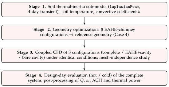
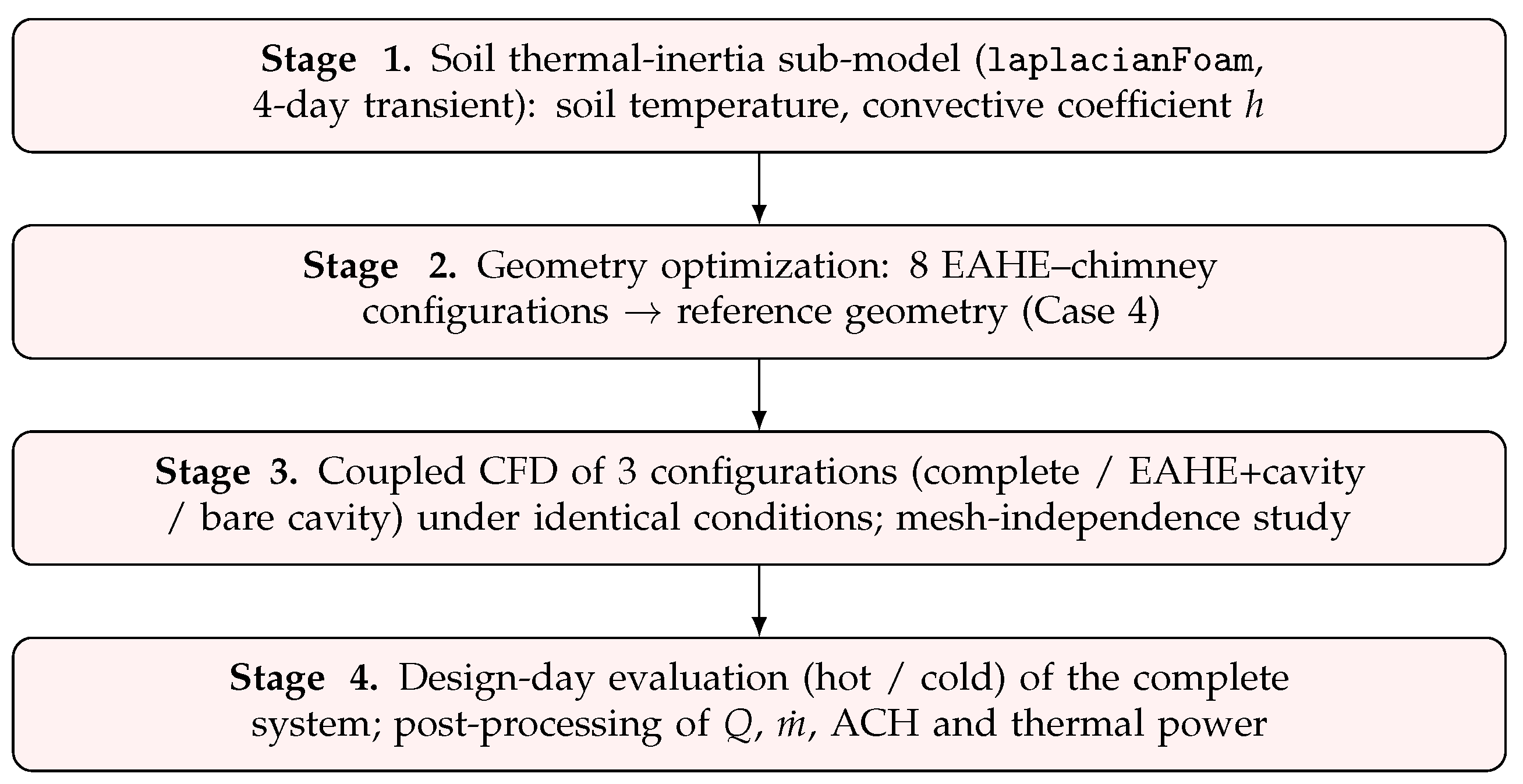
This section describes the methodology used to evaluate the thermal performance of the coupled physical model (EAHE + single-channel solar chimney + cavity). It first introduces the governing equations used to model heat transfer and fluid flow, followed by the optimization procedure applied to define the coupling geometry. Subsequently, the computational domain, the mesh generation strategy, its independence study, and the boundary conditions are described, followed by model validation. The performance indicators used to assess the system are then presented. Finally, a design-day evaluation was conducted considering representative hot and cold conditions to analyze the system performance in different climatic scenarios. A four-stage methodology flow chart is shown in Figure 1, and the complete software environment is summarized in Section 2.6 for reproducibility.

2.1. Physical Model and Case Definition

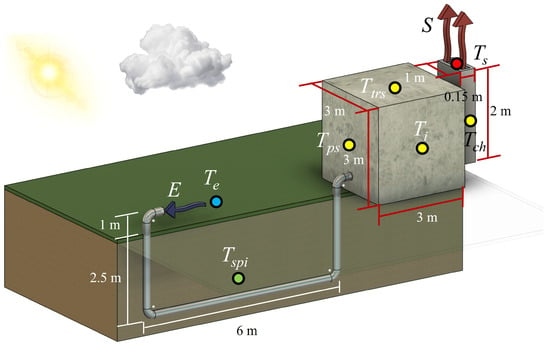
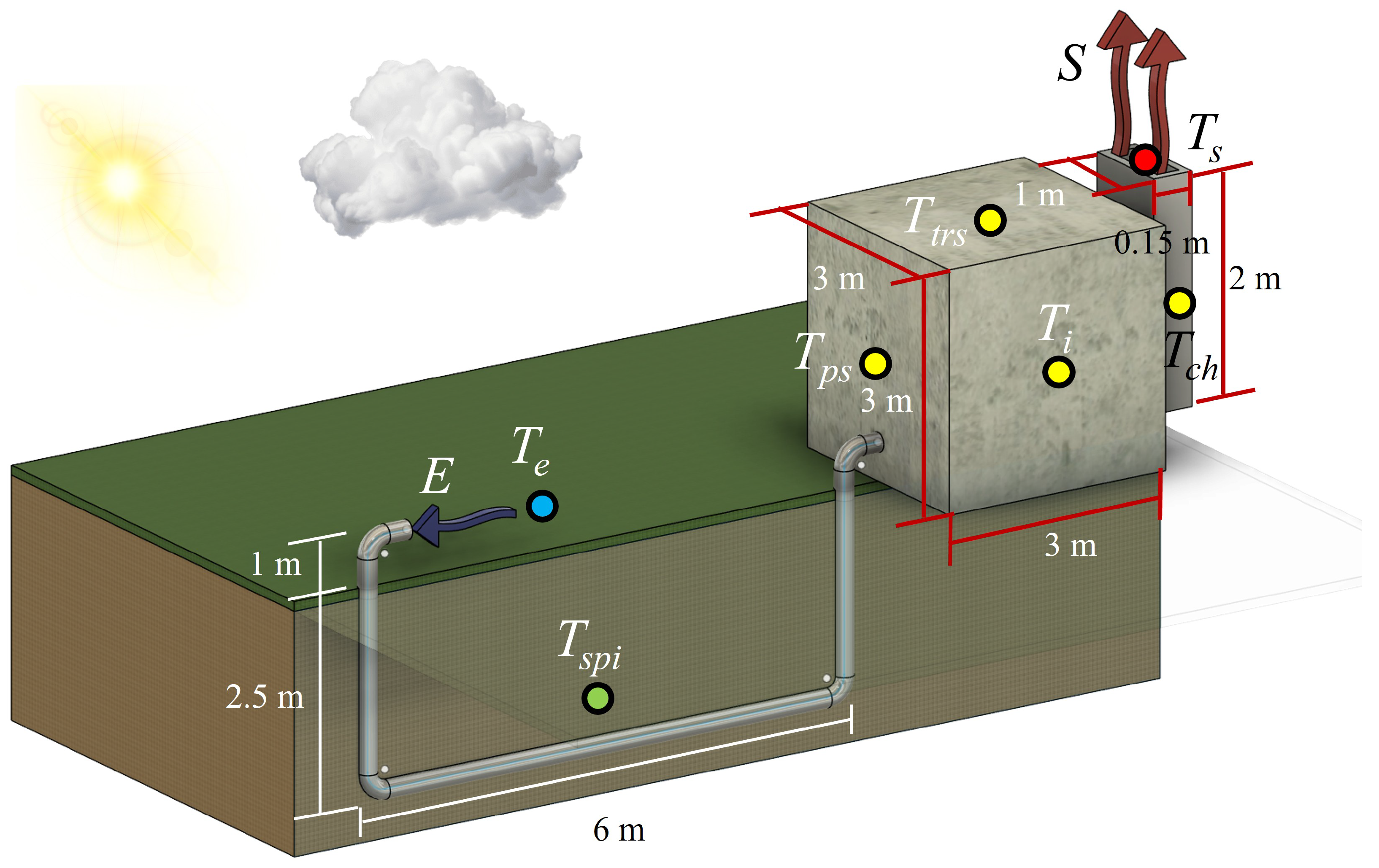
The physical model is based on the full-scale experimental EAHE reported by Díaz-Hernández et al. [10] for warm–humid conditions. The exchanger consists of a 4-inch (0.1016 m) diameter conduit, 6 m long, buried 2.5 m below the surface (Figure 2); this depth was selected because daily fluctuations in soil-temperature become negligible below 2 m [8,10]. The duct feeds a cubic cavity of $3\times 3\times 3$ m (27 m³) that represents the interior of the home, dimensioned according to the recommendations for indoor-air-quality and ventilation and consistent with previous studies of the coupled-system. This $3\times 3\times 3$ m cavity was adopted because it is the reference room size used in comparable coupled EAHE–solar-chimney studies [23,24,26,27], which facilitates comparison with the literature. Because ACH and mean temperature are intensive quantities, conclusions on relative performance can be transferred to larger rooms provided the input/outlet areas are scaled proportionally to the volume of the room; the absolute ventilation of a larger room would require correspondingly larger openings, as discussed in Section 4. The cavity is connected to a single-channel solar chimney with a base $1\mathrm{m}\times 0.15\mathrm{m}$ and a height of 2 m, following the recommendations of Villar-Ramos et al. [20]. The corresponding physical outlet cross-section of the chimney channel is therefore $1\mathrm{m}\times 0.15\mathrm{m}=0.15$ m².

Three configurations were solved and compared: (i) the complete system, formed by the EAHE, the cavity, and the solar chimney; (ii) the EAHE + the cavity system, without the solar chimney; and (iii) the bare cavity, used as the reference case. All three cases share the same geometry, mesh strategy, air and soil thermophysical properties, boundary conditions, turbulence model, and solver settings; the only difference is the inclusion or removal of a component so that the differences in the results are attributable solely to the effect of each passive device. In addition, the complete system was evaluated in two contrasting climatic scenarios—a hot and a cold design day—as described in Section 2.8.

2.2. Governing Equations

The airflow is modeled as a steady, incompressible, turbulent flow with buoyancy effects treated through the Boussinesq approximation, in which the density varies linearly with temperature,

$$\rho ={\rho }_0\left[1-\beta \left(T-T_0\right)\right],$$

(1)

where ${\rho }_0$ is the reference density, $\beta$ the thermal-expansion coefficient, $T_0$ the reference temperature, and T the local temperature. These assumptions are consistent with previous numerical investigations of natural convection in enclosed domains, where the Boussinesq approximation has been used successfully to couple the temperature and velocity fields while maintaining computational efficiency [41]. The Reynolds-averaged Navier–Stokes (RANS) equations of mass, momentum, and energy conservation govern the mean flow. For a steady, incompressible, turbulent flow, the conservation of mass, momentum, and energy is expressed, respectively, as

$${\displaystyle \frac{\partial u_i}{\partial x_i}}=0,$$

(2)

$${\displaystyle \frac{\partial \left(u_i{u}_j\right)}{\partial x_j}}=-{\displaystyle \frac{1}{{\rho }_0}}{\displaystyle \frac{\partial p}{\partial x_i}}+{\displaystyle \frac{\partial }{\partial x_j}}\left[(\nu +{\nu }_t)\left({\displaystyle \frac{\partial u_i}{\partial x_j}}+{\displaystyle \frac{\partial u_j}{\partial x_i}}\right)\right]+g_i\beta (T-T_0),$$

(3)

$${\displaystyle \frac{\partial \left(u_{j}T\right)}{\partial x_j}}={\displaystyle \frac{\partial }{\partial x_j}}\left[(\alpha +{\alpha }_t){\displaystyle \frac{\partial T}{\partial x_j}}\right],$$

(4)

where $u_i$ are the mean velocity components, p the pressure, $g_i$ the gravitational acceleration, $\nu$ and ${\nu }_t$ the molecular and turbulent (eddy) kinematic viscosities, and $\alpha$ and ${\alpha }_t$ the molecular and turbulent thermal diffusivities; the last term of Equation (3) is the buoyancy force introduced through the Boussinesq approximation, Equation (1). The RANS approach offers an adequate compromise between computational cost and accuracy compared to direct numerical simulation (DNS) or Large-Eddy Simulation (LES), which require prohibitively fine meshes [42,43,44].

Turbulence closure is provided by the standard k–$\epsilon$ model, widely validated for fully developed internal flows and natural-ventilation applications due to its numerical robustness and low computational cost [45]. The model solves two transport equations, one for the turbulent kinetic energy k and one for its dissipation rate $\epsilon$:

$${\displaystyle \frac{\partial \left(\rho u_{i}k\right)}{\partial x_i}}={\displaystyle \frac{\partial }{\partial x_j}}\left[\left(\mu +{\displaystyle \frac{{\mu }_t}{{\sigma }_k}}\right){\displaystyle \frac{\partial k}{\partial x_j}}\right]+G_k+G_b-\rho \epsilon ,$$

(5)

$${\displaystyle \frac{\partial \left(\rho u_i\epsilon \right)}{\partial x_i}}={\displaystyle \frac{\partial }{\partial x_j}}\left[\left(\mu +{\displaystyle \frac{{\mu }_t}{{\sigma }_{\epsilon }}}\right){\displaystyle \frac{\partial \epsilon }{\partial x_j}}\right]+C_{1\epsilon }{\displaystyle \frac{\epsilon }{k}}\left(G_k+C_{3\epsilon }{G}_b\right)-C_{2\epsilon }\rho {\displaystyle \frac{{\epsilon }^2}{k}},$$

(6)

where ${\mu }_t$ is the turbulent viscosity, ${\sigma }_k$ and ${\sigma }_{\epsilon }$ are the turbulent Prandtl numbers for k and $\epsilon$, and $G_k$ and $G_b$ are the production of turbulent kinetic energy due to mean velocity gradients and buoyancy, respectively. The wall regions were treated with standard wall functions consistent with the high-Reynolds-number formulation of the k–$\epsilon$ model (nutkWallFunction for turbulent viscosity, and kqRWallFunction and epsilonWallFunction for k and $\epsilon$). Based on the EAHE operating conditions (mean duct velocity of 0.9218 m s⁻¹, $D_h=0.1016$ m and $\nu =1.60\times {10}^{-5}$ m² s⁻¹), the Reynolds number is $Re\approx 5.85\times {10}^3$, i.e., a low-turbulent, fully developed regime for which the standard k–$\epsilon$ model with wall functions has been extensively applied to EAHE and solar-chimney flows [29,45].

2.3. Thermal Inertia of the Soil

As a preliminary stage, the transient thermal behavior of the soil surrounding the buried duct was analyzed with the OpenFOAM solver laplacianFoam, which solves the transient heat-conduction Equation (Laplace-type) for a scalar temperature field,

$${\displaystyle \frac{\partial T}{\partial t}}=\alpha {\nabla }^{2}T+S,$$

(7)

where $\alpha$ is the thermal diffusivity and S an optional heat source/sink. The thermal diffusivity of the soil was taken from the literature [18], and the domain was initialized at a uniform temperature of 27.7 °C, corresponding to the average soil temperature at 2.5 m reported for the reference site [10]. It is important to note that, unlike temperate climates where the soil temperature at 2.5 m is typically 10–15 °C, the study site is located in Tabasco, Mexico, a warm–humid tropical climate with a high mean annual air temperature and a shallow water table. The undisturbed soil temperature at 2.5 m at this site was measured experimentally over one year by Díaz-Hernández et al. [10] and remains close to 27–28 °C; the value adopted here is therefore taken directly from that site-specific experimental campaign and not from generic temperate-climate correlations. Consequently, the EAHE does not exploit a large soil-to-air temperature difference but rather the thermal stability of the ground: it damps the diurnal and seasonal swings of the outdoor air (which can exceed 40 °C on hot days) toward the stable ∼28 °C of the deep soil, which is the mechanism responsible for the cooling reported below. Transient boundary conditions were imposed by means of polynomials fitted to experimental temperature data,

$$T\left(t\right)={\displaystyle \sum _{i=0}^5}{a}_i{t}^i+bsin\left({\displaystyle \frac{2\pi t}{\mathrm{86,400}}}\right)+c,$$

(8)

in which the polynomial term captures the general trend of the soil temperature and the sinusoidal term reproduces the 24 h diurnal cycle (period 86,400 s). Dirichlet conditions were applied at the upper and lower soil surfaces, a third-kind (convective) condition at the duct walls, adiabatic conditions at the lateral boundaries, and symmetry conditions at the domain ends. Polynomial coefficients are listed in

Table 1. Coefficients of the boundary-condition polynomials, Equation (8).

Coef.	1st Kind (Top)	1st Kind (Bottom)	3rd Kind (Duct Walls)
$a_0$	28.331773	27.670981	28.236825
$a_1$	$-1.778535\times {10}^{-5}$	$3.142183\times {10}^{-8}$	$-4.461869\times {10}^{-6}$
$a_2$	$1.169548\times {10}^{-10}$	$-4.919981\times {10}^{-13}$	$7.774422\times {10}^{-11}$
$a_3$	$-2.636024\times {10}^{-16}$	$2.310189\times {10}^{-18}$	$-2.149831\times {10}^{-16}$
$a_4$	$2.314148\times {10}^{-22}$	$-3.663839\times {10}^{-24}$	$2.043781\times {10}^{-22}$
$a_5$	$-6.898478\times {10}^{-29}$	$1.619846\times {10}^{-30}$	$-6.339628\times {10}^{-29}$
b	1.51	0.025	3.12
c	1	1	0.87

. The coefficients are reported with the number of significant figures of the original polynomial fit; the physical temperatures derived from them are quoted to one–two decimals consistent with the resolution of the experimental data [10].

The convective heat-transfer coefficient at the duct wall was obtained from the dimensionless Prandtl, Reynolds, and Nusselt numbers,

$$Pr={\displaystyle \frac{\nu }{\alpha }}={\displaystyle \frac{\mu c_p}{k}},Re={\displaystyle \frac{v{D}_h}{\nu }},Nu=0.023R{e}^{0.8}P{r}^n,h={\displaystyle \frac{Nuk}{D_h}},$$

(9)

where the Nusselt number was estimated from the Dittus–Boelter correlation for turbulent tube flow [46,47,48]. Because the air is being cooled by the surrounding ground, the exponent $n=0.3$ was adopted, as prescribed by the Dittus–Boelter correlation for a fluid that is cooled. With $Re\approx 5.85\times {10}^3$ (>4000, turbulent) and $Pr\approx 0.71$, the air properties at the mean temperature of 28.24 °C (

Table 2. Thermophysical properties of air at the mean temperature of 28.24 °C.

Property	Value
Density, $\rho$ (kg m−3)	1.1568
Specific heat, $c_p$ (J kg−1K−1)	1007.056
Dynamic viscosity, $\mu$ (N s m−2)	$1.8526\times {10}^{-5}$
Thermal conductivity, k (W m−1K−1)	0.026403
Thermal diffusivity, $\alpha$ (m2 s−1)	$2.2665\times {10}^{-5}$
Kinematic viscosity, $\nu$ (m2 s−1)	$1.6015\times {10}^{-5}$

) and a hydraulic diameter $D_h=0.1016$ m yield a convective coefficient $h=5.73$ W m⁻²°C⁻¹. The simulation was run for a period of four days, and the soil domain was discretized with an unstructured 3D mesh (0.02–0.15 m element size; 26,201 nodes, 129,753 tetrahedra) refined around the duct curvature [49].

2.4. Optimization of the Coupling Geometry

Before coupled CFD simulations, eight geometrical configurations were evaluated to determine the best relative position of the EAHE inlet and the solar-chimney outlet with respect to the cavity by varying the connection distances B (EAHE) and A (chimney). The objective criterion was to minimize the mean air temperature in the cavity (both in the entire cavity and in a representative Section 2 m above the floor), which is the main passive-cooling target. The geometry and thermal results of all eight configurations are summarized in

Table 3. Geometric parameters and thermal results of the eight coupling configurations evaluated (B: EAHE connection distance; A: chimney connection height). The objective criterion is the mean cavity temperature; Case 4 (in bold) was selected.

Case	B (m)	A (m)	${\mathit{T}}_{\mathbf{avg}}$ Cavity (°C)	${\mathit{T}}_{\mathbf{avg}}$ at 2 m (°C)	Exec. Time (h)
1	1.00	1.0	33.6	33.3	17.13
2	1.50	1.0	33.7	33.6	30.51
3	2.00	1.0	33.7	33.9	48.94
4	0.25	2.0	33.2	32.7	29.43
5	0.50	2.0	33.4	33.0	51.57
6	1.00	2.0	33.4	33.0	69.01
7	1.50	2.0	33.6	33.5	26.53
8	2.00	2.0	33.6	33.8	35.59

. The mean cavity temperatures ranged from 33.2 °C to 33.7 °C, and between 32.7 °C and 33.9 °C in a Section 2 m above the floor. Configuration 4—the EAHE inlet located 0.25 m from the cavity base and the chimney outlet at a 2 m height—produced the lowest average temperatures and the most efficient EAHE–chimney interaction and therefore was adopted as the best-performing configuration among the eight tested cases and used as a reference geometry for all subsequent simulations.

2.5. Computational Domain, Mesh and Boundary Conditions

To reduce computational cost without affecting the physical representativeness of the model, the domain was simplified by cutting the symmetry, reducing the depth of the cavity and chimney to a thickness of 0.20 m while preserving the trajectory, length, and diameter of the EAHE. A symmetry condition was imposed on the front plane and an empty condition on the back plane so that the governing equations were solved only in the plane of interest, yielding a quasi-two-dimensional representation of the flow at a considerably lower cost.

The relationship between the computational and the physical domains is summarized below. The physical cavity is $3\times 3\times 3$ m ($V_{\mathrm{phys}}=27$ m³) with a chimney outlet of $0.15\mathrm{m}\times 1\mathrm{m}=0.15$ m²; the reduced computational slice keeps the same height and length but a depth of $d=0.20$ m, giving a computational cavity volume $V_{2\mathrm{D}}=3\times 3\times 0.20=1.8$ m³ and a computational outlet area $A_{2\mathrm{D}}=0.15\times 0.20=0.03$ m². Because ACH is the ratio of the volumetric flow from the outlet to the enclosed volume, and both the outlet area and the volume scale linearly with the eliminated depth d,

$$\mathrm{ACH}={\displaystyle \frac{\overline{v}{A}_{\mathrm{out}}3600}{V_{\mathrm{cav}}}}={\displaystyle \frac{\overline{v}\left(0.15d\right)3600}{9d}}={\displaystyle \frac{\overline{v}\left(0.15\right)3600}{9}},$$

(10)

the depth d cancels out. Consequently, the ACH computed on the quasi-2D slice is identical to that of the full 27 m³ room, and the mean temperatures (intensive quantities) are likewise preserved. The ACH values reported for the three configurations (Section 3) were obtained with $A_{2\mathrm{D}}=0.03$ m² and $V_{2\mathrm{D}}=1.8$ m³ and therefore correspond to the physical room. Only the EAHE duct, which retains its true circular cross-section, transports the physically dimensional duct flow rate reported in Section 3.5. It should nevertheless be acknowledged that the quasi-two-dimensional simplification neglects three-dimensional flow and temperature effects (such as lateral recirculation and corner effects) present in the actual room; the reported values should therefore be interpreted as representative of the mid-plane behavior, and a fully three-dimensional simulation is recommended as future work.

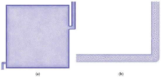
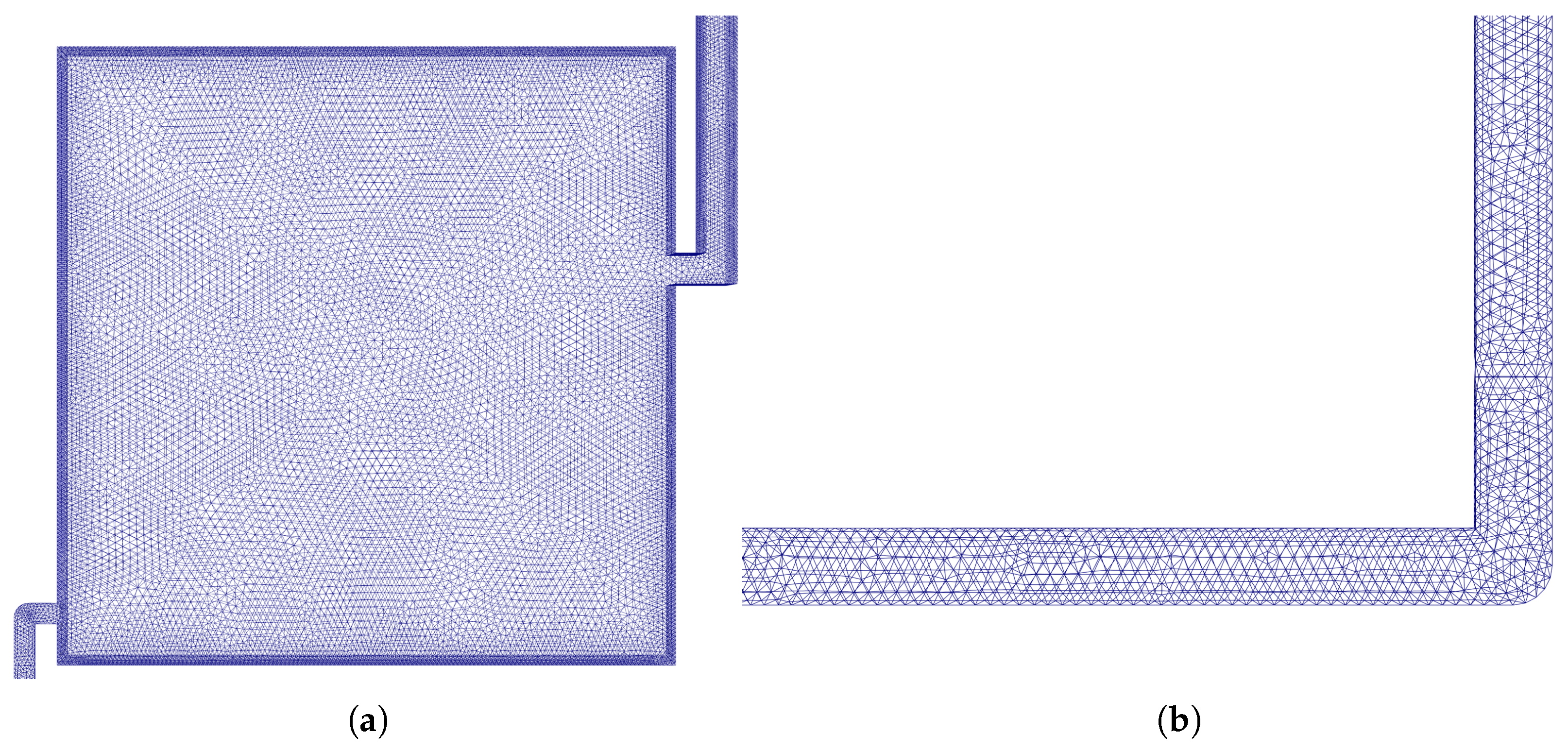
The coupled domain was meshed in Salome using the unstructured NetGen algorithm with tetrahedral elements. A base size between 0.006 m (minimum) and 0.04 m (maximum) was used, with local refinement down to 0.003 m near the EAHE walls and elbows, 0.005 m inside the solar chimney and 0.01 m in the connecting cavity, to resolve steep thermal gradients and buoyancy-driven ascending flow (Figure 3).

A mesh-independence study was carried out for the coupled domain using three refinement levels (coarse, medium, and fine). For each mesh, the pseudo-transient evolution of the mean air temperature in a representative cavity region (1 m above the floor) was monitored until it reached an asymptotic value.

Table 4. Mesh-independence study for the coupled domain (mean air temperature monitored 1 m above the cavity floor).

Mesh	Cells	Comp. Time (h)	Mean Cavity T (1 m) (°C)
Coarse	85,875	1.14	32.02
Medium (selected)	133,933	6.76	32.84
Fine	398,396	18.83	32.26

reports the cell count, the computational time, and the resulting temperature. The solution converges asymptotically with refinement, and the medium mesh (133,933 cells) was selected as the definitive configuration because it captures buoyancy-driven convection and vertical thermal gradients at a substantially lower cost than the fine mesh. This medium mesh was used for all coupled simulations reported below. Although the independence metric tabulated here is the mean cavity temperature, the flow-related outputs were also monitored during the study: the maximum velocity and the outlet volumetric flow reached practically constant values upon refinement (consistent with the convergence of the residuals), indicating that the ventilation-related quantities (outlet flow and ACH) are likewise insensitive to further refinement. A dedicated per-mesh tabulation of the outlet flow and ACH was not carried out, which is acknowledged as a limitation.

The EAHE duct was segmented to assign first-kind (fixed-temperature) boundary conditions from experimental data, complemented by temperatures prescribed at the cavity roof and walls and at the solar-chimney glass and interior surfaces. The wall temperatures for the hottest and coldest design days were estimated with a previously validated global energy-balance tool [50]. Two flow-driving conditions were used according to the objective of each stage. For the comparison of three-configurations under the design condition (Section 3), a fixed EAHE inlet velocity of 0.9218 m s⁻¹ was prescribed, following the experimental reference of forced-convection of Díaz-Hernández et al. [10]; this provides a controlled, identical supply condition for the three cases so that the differences are attributable only to the presence/absence of each component. For the design-day evaluation of the complete system (Section 2.8), no inlet velocity was imposed: the flow was left to develop solely from buoyancy (natural convection), using pressureInletOutletVelocity at the openings so that the coupling between the EAHE and the solar chimney emerges from the density field rather than from a prescribed velocity. The main boundary temperatures for the hot design condition are summarized in

Table 5. Main temperature boundary conditions prescribed in the coupled model (hot design condition).

Element	Type	Value
EAHE inlet	fixedValue	34.76 °C
Chimney outlet	zeroGradient	–
EAHE Section 1	fixedValue	32.15 °C
EAHE Section 2	fixedValue	27.80 °C
EAHE Section 3	fixedValue	28.00 °C
EAHE Section 4	fixedValue	28.10 °C
EAHE Section 5	fixedValue	27.70 °C
Cavity roof	fixedValue	35.40 °C
Cavity north wall	fixedValue	33.50 °C
Cavity south wall	fixedValue	33.30 °C
Solar chimney (glass)	fixedValue	49.00 °C
Solar chimney (interior)	fixedValue	68.50 °C
Front plane (whole model)	symmetry	–
Cavity/chimney back plane	empty	–

.

2.6. Solver Configuration and Reproducibility

The coupled simulations were performed with the OpenFOAM solver buoyantSimpleFoam  for the forced-convection design condition and buoyantBoussinesqSimpleFoam for the natural-convection design-day cases, designed for steady, turbulent flow with heat transfer and buoyancy effects through the Boussinesq approximation. The controlDict file specified a steady run between 0 and 200 s, with an initial time step of 0.005 s, automatic adjustment to keep a maximum Courant number of 0.2 (maximum step 0.008 s) and residual monitoring enabled. In fvSchemes, a steadyState time scheme was used, with Gauss linear gradients, bounded Gauss upwind divergence terms, and Gauss linear orthogonal Laplacians. In fvSolution, the modified pressure $p_{rgh}$ was solved with the PCG solver (DIC preconditioner, absolute tolerance $1\times {10}^{-8}$), while velocity, turbulence quantities and energy used PBiCGStab with a DILU preconditioner; pressure–velocity coupling was handled with the SIMPLE algorithm, with relaxation factors of 0.7 (pressure), 0.2 (velocity) and 0.1 (energy). The thermophysical model was heRhoThermo with a pureMixture and the Boussinesq approximation ($M=28.9$, ${\rho }_0=1$ kg m⁻³, $T_0=300$ K, $\beta =3\times {10}^{-3}$K⁻¹, $c_v=712$ J kg⁻¹K⁻¹, $\mu =1\times {10}^{-5}$ Pa s, $Pr=0.7$), and turbulence was modeled with the RAS k–$\epsilon$ model. Convergence was verified by monitoring the residuals of velocity, pressure, and temperature and the global mass balance; the momentum, energy and turbulence residuals dropped below ${10}^{-6}$ and the pressure residual below ${10}^{-5}$, and the maximum velocity and outlet volumetric flow reached constant values.

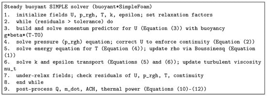
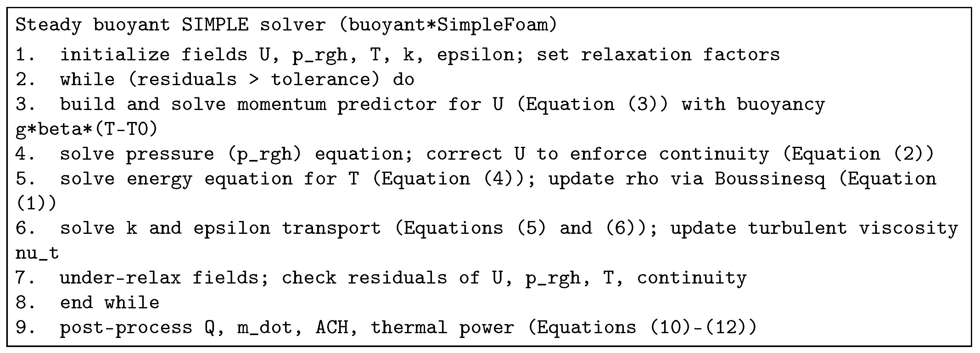
For reproducibility, the complete software environment was: OpenFOAM (The OpenFOAM Foundation) v12 [37] for the CFD solution, Salome (NetGen algorithm) for mesh generation, ParaView 5.8.0 for field post-processing, and Python 3 (NumPy, pandas, Matplotlib and openpyxl) for the section-based reduction of the design-day indicators. The steady buoyant SIMPLE procedure used in this study is summarized in Figure 4.

2.7. Performance Indicators

The results were post-processed with ParaView 5.8.0. A cross-section normal to the flow was extracted with the Slice filter; its area was obtained with Integrate Variables, and the mean temperature and velocity with Descriptive Statistics. The volumetric flow rate was computed from the continuity equation for incompressible flow and the air mass flow rate from

$$Q=A\overline{v},\dot{m}=\rho Q.$$

(11)

Consistent with the Boussinesq formulation of the coupled model, the density used in Equation (11) is the Boussinesq density evaluated at the local mean temperature, $\rho ={\rho }_0[1-\beta (T-T_0)]$ with ${\rho }_0=1$ kg m⁻³, $T_0=300$ K and $\beta =3\times {10}^{-3}$K⁻¹; at the EAHE outlet temperature this gives $\rho \approx 0.99$ kg m⁻³. This is the density that reconciles the mass and volumetric flow rates reported in Section 3.5 (e.g., $23.71$ m³ h⁻¹$=6.59\times {10}^{-3}$ m³ s⁻¹, and $\dot{m}=0.99\times 6.59\times {10}^{-3}=6.52\times {10}^{-3}$ kg s⁻¹). The value $\rho =1.1568$ kg m⁻³ listed in Table 2 corresponds to the reference properties used only for the convective-coefficient (h) calculation of the soil sub-model and is not used in the coupled mass balance. The ventilation capacity was quantified through the number of air changes per hour,

$$\mathrm{ACH}={\displaystyle \frac{Q_{\mathrm{out}}\times 3600}{V_{\mathrm{cav}}}},$$

(12)

where $V_{\mathrm{cav}}$ is the volume of the cavity and $Q_{\mathrm{out}}$ is the volumetric flow of the outlet. The thermal power removed by the EAHE and by the cavity was evaluated from the steady-flow energy balance,

$$\dot{Q}=\dot{m}{c}_p\Delta T,$$

(13)

where $\Delta T$ is the temperature difference between the inlet and outlet of the corresponding control volume. It should be emphasized that ${\dot{Q}}_{\mathrm{EAHE}}$ (evaluated with $\Delta T_{\mathrm{EAHE}}<0$ on a hot day) represents sensible heat extracted from the supply air by the ground, whereas ${\dot{Q}}_{\mathrm{SC}}$ represents sensible heat gained by the air inside the solar chimney from solar radiation. These two quantities act on different air streams and have opposite thermodynamic meaning; therefore, they are reported separately and are not added into a single “cooling power” delivered to the building. The chimney heat gain is the driver of the buoyancy flow, not a cooling contribution. Finally, to compare the relative magnitude of the ground-cooling effect and the chimney driving gradient in the design-day analysis, a dimensionless relative thermal-contribution ratio was defined as

$$R_{\Delta T}={\displaystyle \frac{|\Delta T_{\mathrm{EAHE}}|}{|\Delta T_{\mathrm{SC}}|}}\times 100\%.$$

(14)

This ratio is not a heat-exchanger effectiveness in the classical ($\epsilon$–NTU) sense; it is simply an indicator of which mechanism dominates the thermal response for a given design day.

2.8. Design-Day Evaluation: Hot and Cold Conditions

To assess the behavior of the entire system under contrasting climatic demands, two additional steady-state simulations were carried out under the boundary conditions corresponding to a representative hot and a representative cold day of a typical year, obtained with the validated global energy-balance tool [50]. These are two representative steady design-day conditions and do not constitute a transient annual simulation. For each scenario, the three-dimensional velocity components ($U_x$, $U_y$, $U_z$) and the temperature were extracted on representative cross-sections of the solar chimney, the cavity and the six EAHE segments, and reduced with a dedicated Python routine. The section velocity magnitude was computed as

$$\overline{v}=\sqrt{{\overline{U_x}}^2+{\overline{U_y}}^2+{\overline{U_z}}^2},$$

(15)

and the indicators of Section 2.7 were evaluated with the outlet velocity taken in the upper chimney section, an outlet area $A_{\mathrm{out}}=0.15$ m² (the physical chimney outlet, $0.15\mathrm{m}\times 1\mathrm{m}$), a cavity volume $V_{\mathrm{cav}}=27$ m³ and constant air properties $\rho =1.225$ kg m⁻³ and $c_p=1005$ J kg⁻¹K⁻¹, with a reference ambient temperature of 20 °C. In an earlier version, this area had been set to an assumed value of $0.30$ m²; it has now been corrected to the physical outlet area of $0.15$ m². Accordingly, we recalculated all affected quantities, including the volumetric and mass flow rates, ACH, renewal time, and thermal powers. The updated values are presented in the corresponding table in Section 3.5. The temperatures and temperature differences are unaffected, and the hot-versus-cold comparison, which depends on the ratio between the two scenarios, is likewise unchanged. This design-day analysis quantifies how the ventilation and the thermal-energy exchange of the same physical system respond to opposite climatic demands. Because this evaluation and the comparison of three-configurations use different post-processing conventions, their absolute ventilation magnitudes are not directly interchangeable; therefore, the two studies are interpreted independently and a unified single-convention post-processing is identified as future work (Section 4).

2.9. Model Verification and Consistency Check

The EAHE sub-model (the earth–air heat exchanger without the solar chimney) was verified against the full-scale experimental data of Díaz-Hernández et al. [10], obtained at the same warm–humid site (Tabasco, Mexico) over one year of monitoring, which is the reference used to define the physical model. The experimental campaign reported an air-temperature reduction of EAHE (cooling potential) of up to 5.5 °C under summer conditions. The present CFD model reproduces this behavior: the computed air-temperature reduction across the EAHE is 5.75 °C for the hot design day and 4.75–6.81 °C for the design-condition cases, i.e., the same order and trend as the experiment, with a difference of about 4.5% for the hot design day (5.75 vs. 5.5 °C), as summarized in

Table 6. Verification of the EAHE sub-model against the experimental cooling potential reported for the same site by Díaz-Hernández et al. [10].

Quantity	Experimental [10]	Present CFD (EAHE)	Difference
EAHE air-temperature reduction (hot/summer)	up to 5.5 °C	5.75 °C (hot design day)	≈4.5%
EAHE air-temperature reduction (design cases)	2.8–5.5 °C [10]	4.75–6.81 °C	same order/trend

. This comparison should be regarded as a consistency check against the reported experimental cooling potential rather than a matched, one-to-one validation case because the experimental and numerical boundary conditions are not identical; it therefore supports the consistency of the EAHE sub-model with the experimental data but does not constitute a full validation of the coupled system. A complete point-by-point validation of the fully coupled EAHE–cavity–solar-chimney model against dedicated experimental measurements is in progress and is identified as future work.

3. Results

This section presents the numerical results of the proposed passive conditioning system. The analysis begins with the evaluation of the thermal inertia of the surrounding soil, followed by a comparison of the thermal and ventilation performance of the three simulated configurations. Finally, the design-day behavior of the complete system is examined under representative hot and cold conditions.

3.1. Analysis of Soil Thermal Inertia

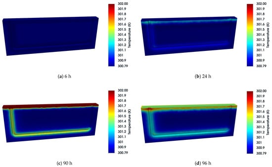
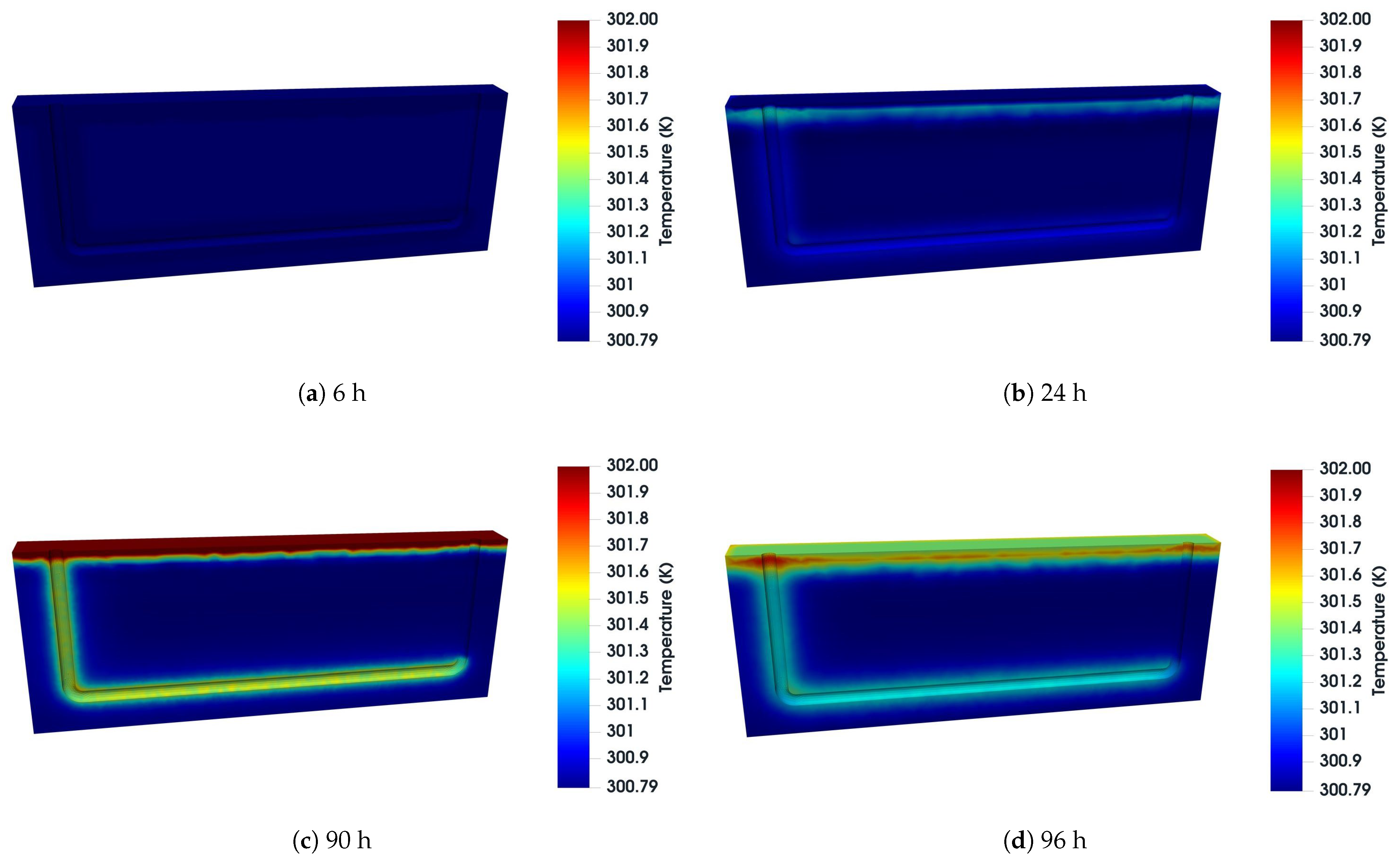
The four-day transient simulation of the soil block (Figure 5) revealed a marked contrast between the surface and the deep soil. The temperature of the soil-surface showed the largest fluctuations, driven by the diurnal cycle, with peaks of up to 28.9 °C at 42 h and 90 h. The air temperature inside the pipe gradually increased, reaching a maximum of 28.32 °C at 90 h, while the temperature of the soil immediately around the pipe remained almost constant (27.65–27.70 °C) throughout the simulation. The small surface-to-depth temperature difference (≈1–2 K in Figure 5) is a direct consequence of the warm–humid tropical setting: in this climate the whole soil column is warm, and the diurnal wave is strongly damped below 2 m, in contrast with temperate climates where a larger surface-to-depth gradient is expected. The reported temperatures (Figure 5) are in kelvin and are consistent with the site-specific experimental data [10]. This behavior demonstrates that the soil at 2.5 m acts as a thermal regulator, damping the extreme surface fluctuations. Within the simulated four-day period, no significant depletion of soil was observed as a heat sink or source; this conclusion is restricted to the simulated period and is consistent with reports that thermal saturation of the surrounding soil may appear only after several days of continuous operation [13], while longer-term soil stability (seasonal/annual) has been reported elsewhere [8].

3.2. Complete System (EAHE + Cavity + Solar Chimney)

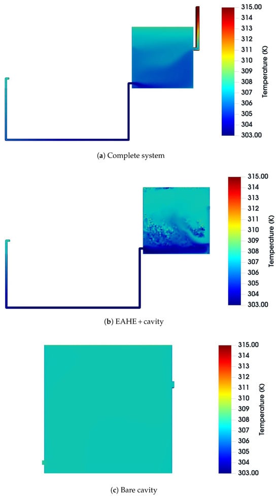
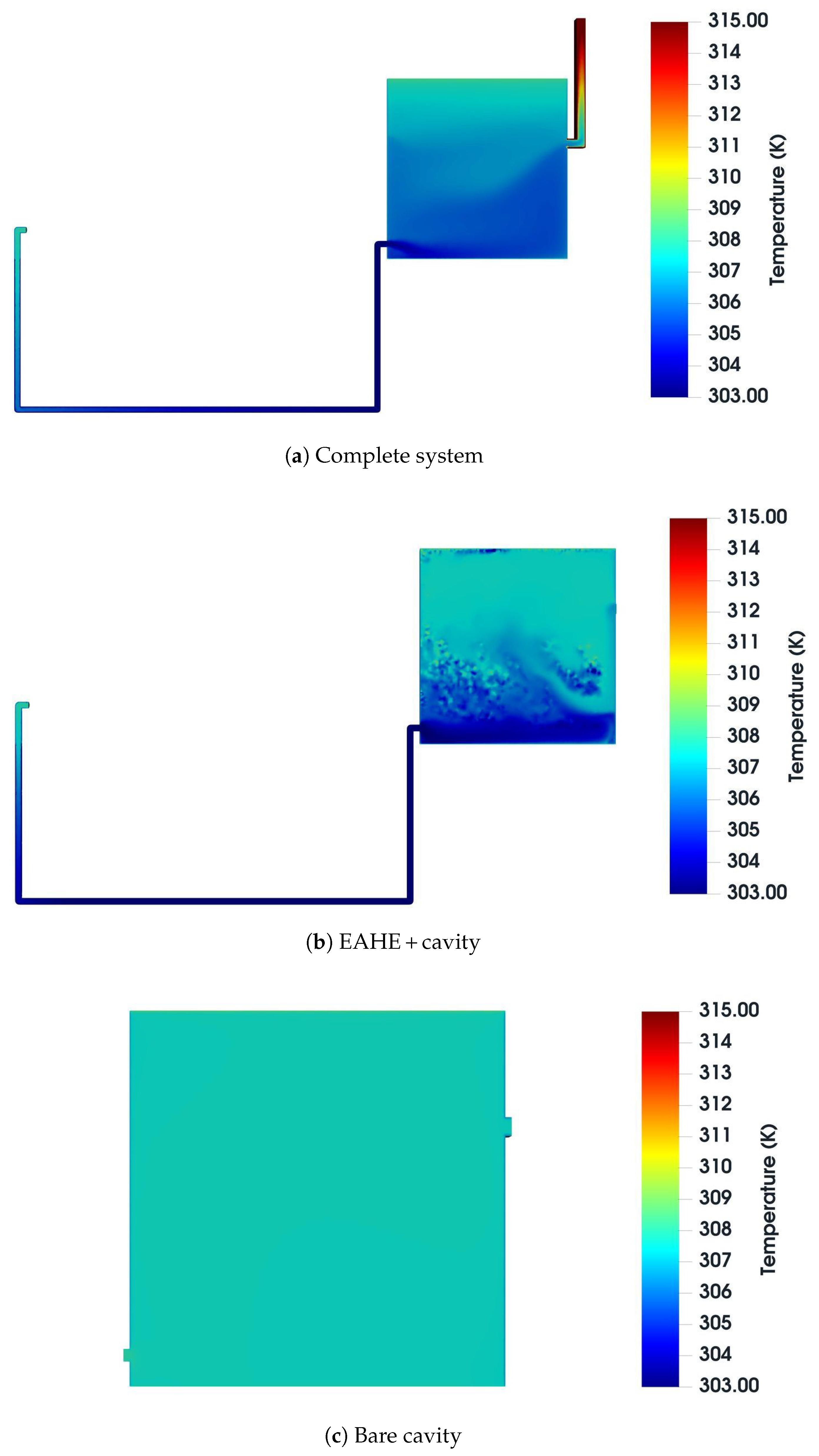
Figure 6a shows the temperature field of the complete system. Air enters the exchanger at about 303 K (the ground boundary temperature) and remains almost uniform along the buried duct. On entering the cavity, the cool jet spreads over the lower region and mixes with the interior air, producing an ascending thermal gradient from roughly 305 K near the floor to approximately 308 K in the upper region, i.e., a natural thermal stratification. The solar chimney reaches the highest temperatures of the system (approximately 315 K) as a consequence of the heating of its exposed surfaces, which reduces the air density and enhances the buoyancy that drives the flow.

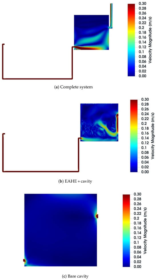
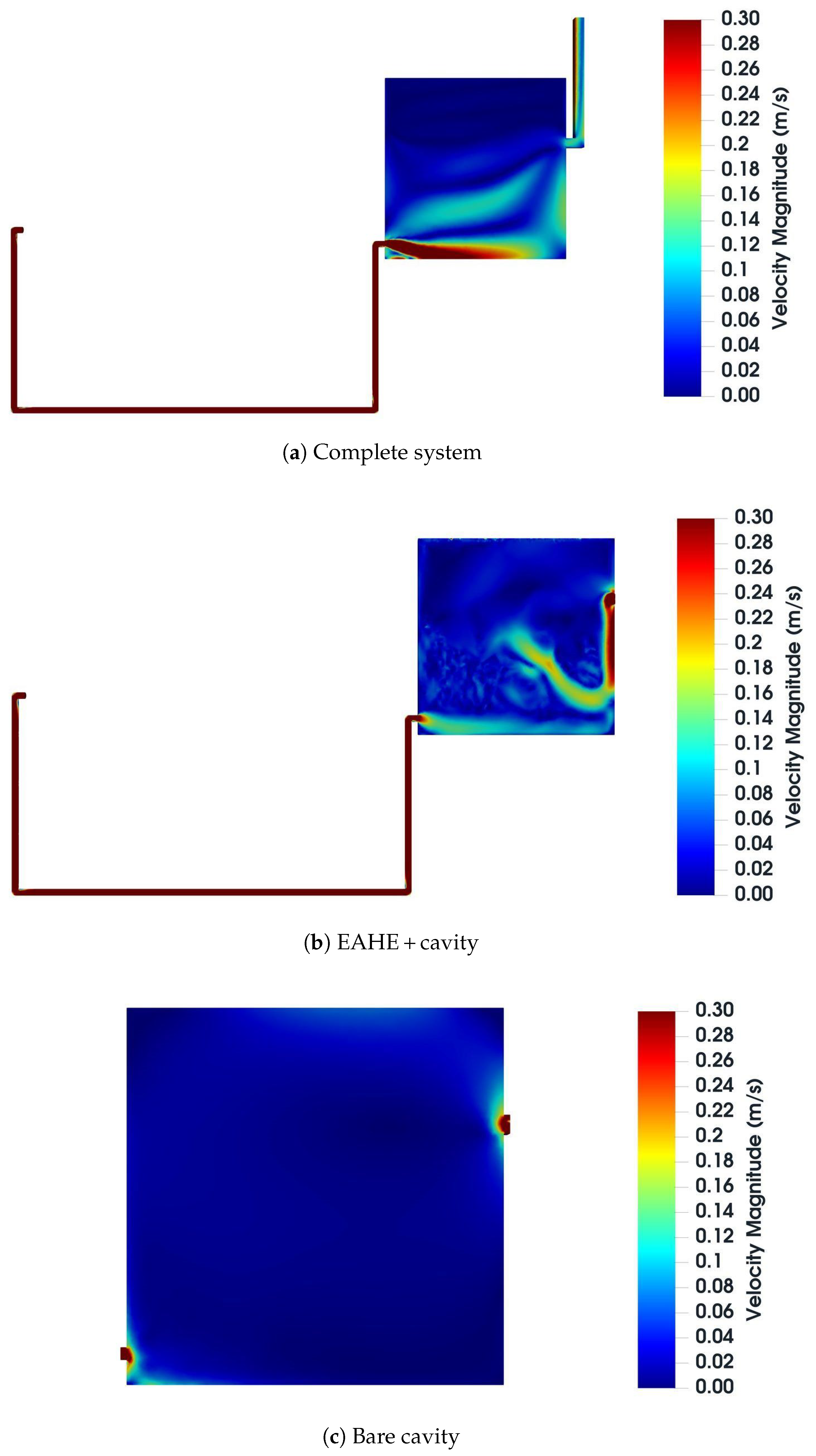
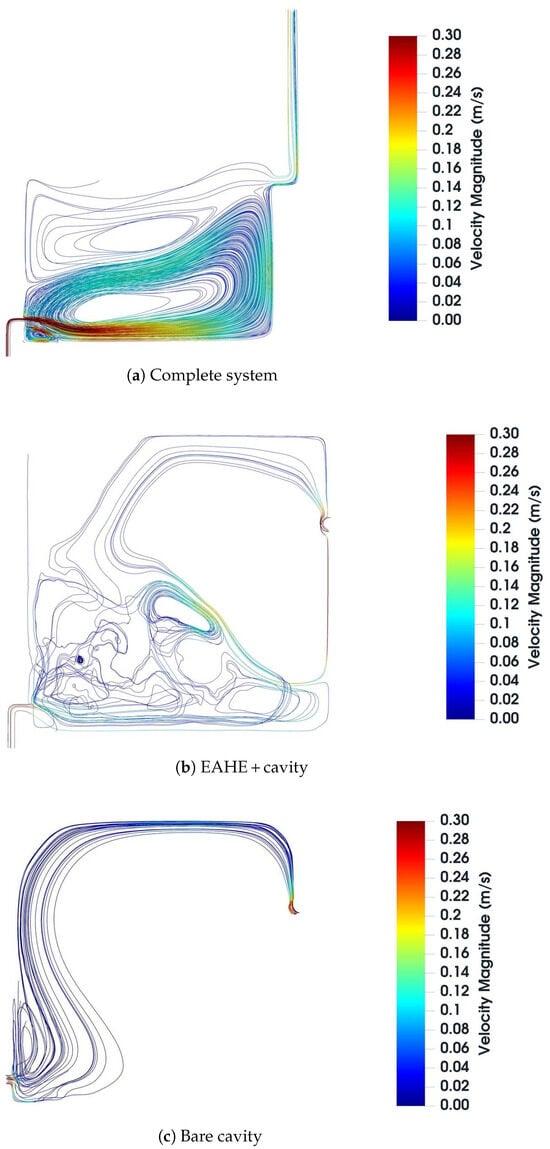
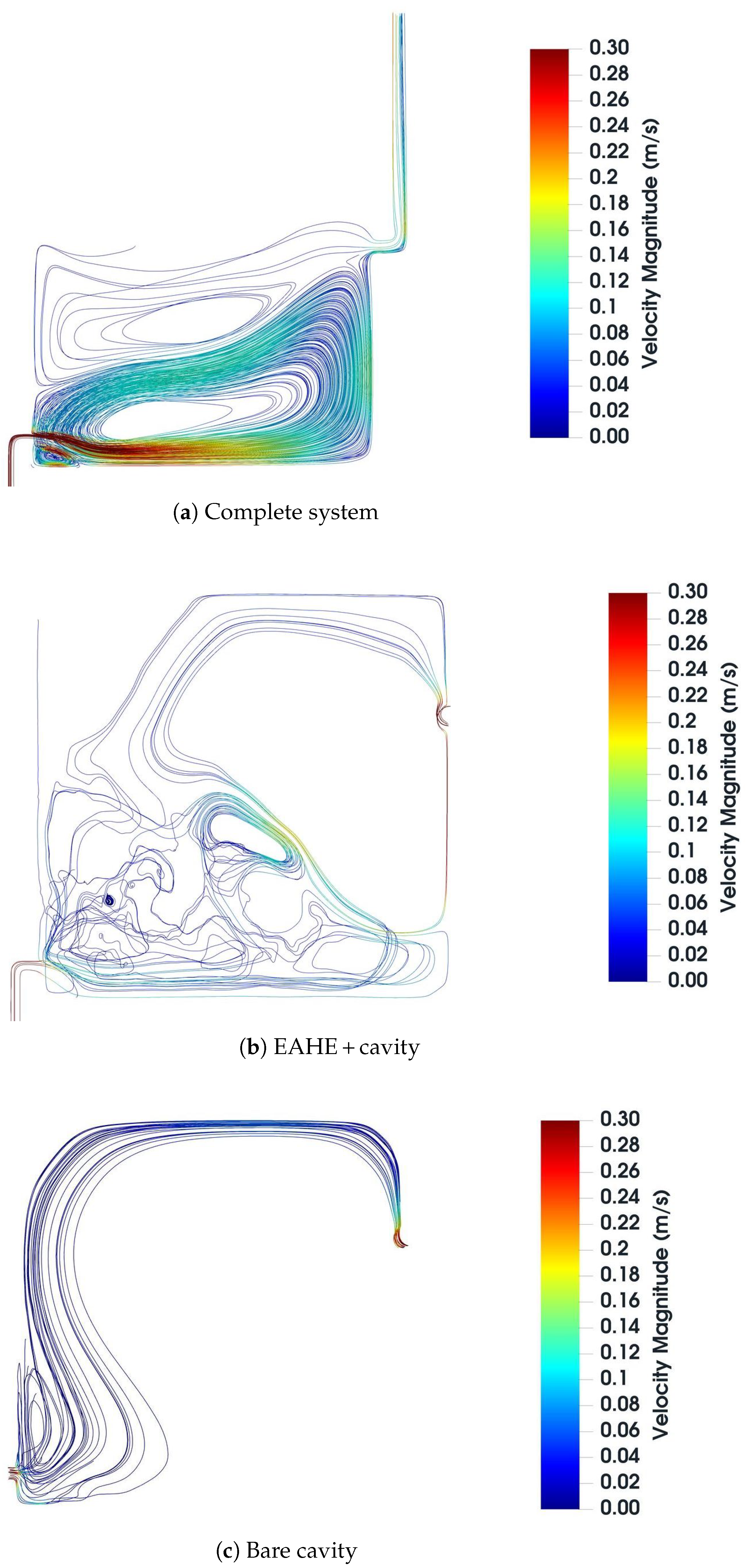
The velocity field (Figure 7a) shows the highest velocities inside the EAHE duct (≈0.30 m s⁻¹) due to its small hydraulic diameter. On entering the cavity the cross-section expands and the velocity drops below 0.10 m s⁻¹, favoring mixing; the cool jet travels along the lower part of the cavity and then rises as it is drawn towards the chimney inlet, where it accelerates again. The streamlines (Figure 8a) confirm the establishment of a continuous circulation loop driven by the density difference between the cold air supply and the heated air in the chimney.

Quantitatively, the EAHE delivered a mean air temperature at the outlet of 30.01 °C, a mean velocity of 0.829 m s⁻¹, a duct volumetric flow rate of 23.71 m³ h⁻¹ and a mass flow rate of 0.00652 kg s⁻¹. This flow rate is the area-averaged value evaluated at the EAHE outlet cross-section (mean velocity 0.829 m s⁻¹ over the post-processing section area of 0.00794698 m²); it is therefore lower than the nominal estimate of ≈26.9 m³ h⁻¹ obtained from the imposed inlet velocity of 0.9218 m s⁻¹ over the full duct area. The difference arises from the local velocity profile and the area-averaging over the section, not from any density effect. The temperature drop across the exchanger was 4.75 °C, corresponding to a sensible cooling power of the supply air of 31.2 W. The mean cavity temperature was 33.20 °C, the outlet velocity was 0.1387 m s⁻¹ and the ventilation rate reached 8.32 ACH, with a thermal power removed from the cavity of 67.04 W.

3.3. EAHE + Cavity System (Without Solar Chimney)

Removing the solar chimney isolates the effect of EAHE. The temperature field (Figure 6b) shows the cool air entering at about 303 K and gradually warming to 307–308 K; without the chimney, the circulation is weaker, and the hot air accumulates in the upper part of the cavity. The velocity field (Figure 7b) confirms the loss of intensity, with recirculation zones and velocities below 0.10 m s⁻¹ in most of the cavity. In this configuration the EAHE reduced the inlet air temperature by 6.81 °C (mean outlet temperature 27.95 °C), with a volumetric flow rate of 10.96 m³ h⁻¹, a removed thermal power of 20.84 W, a mean cavity temperature of 33.45 °C, a ventilation rate of 4.27 ACH and a cavity thermal power of 17.42 W.

3.4. Bare Cavity (Reference Case)

In the bare cavity (Figure 6c and Figure 7c) the temperature field is practically uniform at about 308 K, and the velocity is negligible (<$0.02$ m s⁻¹) over most of the volume. The mean cavity temperature was 34.42 °C, the ventilation rate only 2.01 ACH and the removed thermal power 4.56 W. This case represents the behavior of a house without passive strategies and constitutes a reference to quantify the benefit of the EAHE and the solar chimney.

3.5. Comparative Evaluation of the Three Configurations

Table 7. Comparison of the main performance indicators of the three analyzed configurations (design condition).

Metric	Unit	Complete	EAHE + Cavity	Bare Cavity
EAHE mass flow rate, $\dot{m}$	kg s−1	0.00652	0.00303	0.00319
EAHE duct volumetric flow rate, Q	m3 h−1	23.71	10.96	11.60
Outlet flow rate for ACH, $Q_{\mathrm{out}}$	m3 h−1	14.98	7.69	3.63
Air changes per hour, ACH	h−1	8.32	4.27	2.01
Mean outlet velocity, $\overline{v}$	m s−1	0.1387	0.0712	0.0336
Mean cavity temperature	°C	33.20	33.45	34.42
$\Delta T$ inlet–outlet (EAHE)	°C	4.75	6.81	–
Supply-air cooling power (EAHE)	W	31.2	20.84	–
Thermal power removed (cavity)	W	67.04	17.42	4.56

The outlet flow rate for ACH is $Q_{\mathrm{out}}=\overline{v}{A}_{2\mathrm{D}}$ with $A_{2\mathrm{D}}=0.03$ m², and $\mathrm{ACH}=Q_{\mathrm{out}}3600/V_{2\mathrm{D}}$ with $V_{2\mathrm{D}}=1.8$ m³; as shown in Equation (10), these ACH values also apply to the full 27 m³ room. Synergy indicators: coupling the chimney raises ACH by 94.8% (complete vs. EAHE + cavity) and by 313.9% (complete vs. bare cavity); the isolated EAHE raises ACH by 112.4% (EAHE + cavity vs. bare cavity). The EAHE duct volumetric flow rate corresponds to the area-averaged value at the outlet cross-section, which differs from the nominal inlet-based estimate as explained in Section 3.

summarizes the main performance indicators of the three configurations and the percentage indicators that quantify the contribution of each device. The complete system clearly outperforms the other two: it reaches the lowest mean cavity temperature (33.20 °C), the highest ventilation rate (8.32 ACH) and the highest removed thermal power (67.04 W). The achieved ventilation is also compared with the recommended residential ranges below.

Regarding ventilation adequacy, the ACH achieved by the complete system (8.32 h⁻¹) is well above the minimum outdoor-air ventilation rates typically recommended for residential spaces (of the order of 0.35 h⁻¹ for whole-dwelling ventilation), whereas the bare cavity (2.01 h⁻¹) and the EAHE + cavity case (4.27 h⁻¹) also exceed that threshold but with a much lower renewal capacity. A formal ASHRAE 62.1/62.2 compliance statement is deliberately avoided here because it requires the specific occupancy, floor area and zone-air-distribution data of the target dwelling, which are outside the scope of this numerical study; therefore, ACH values are reported as design indicators rather than as certified compliance.

3.6. Design-Day Performance: Hot and Cold Conditions

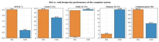
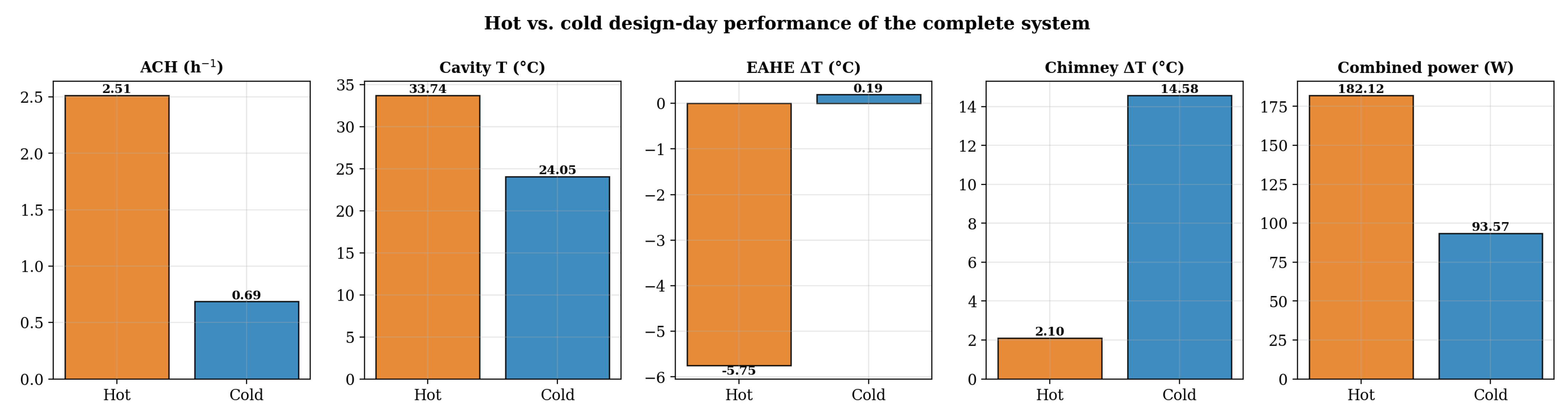
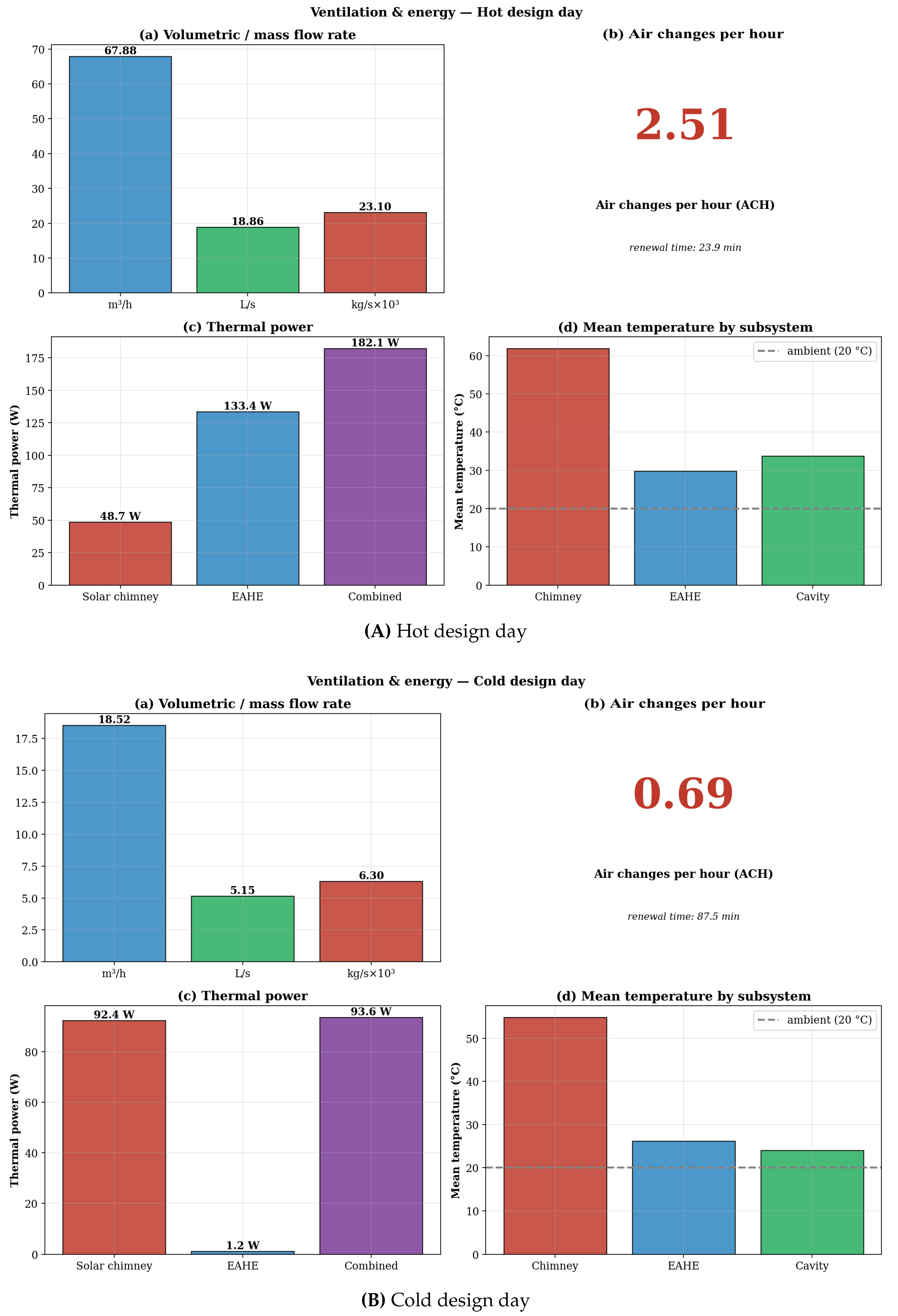
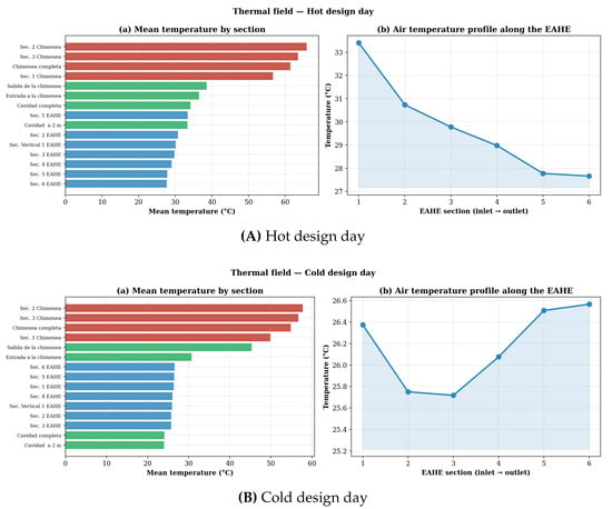
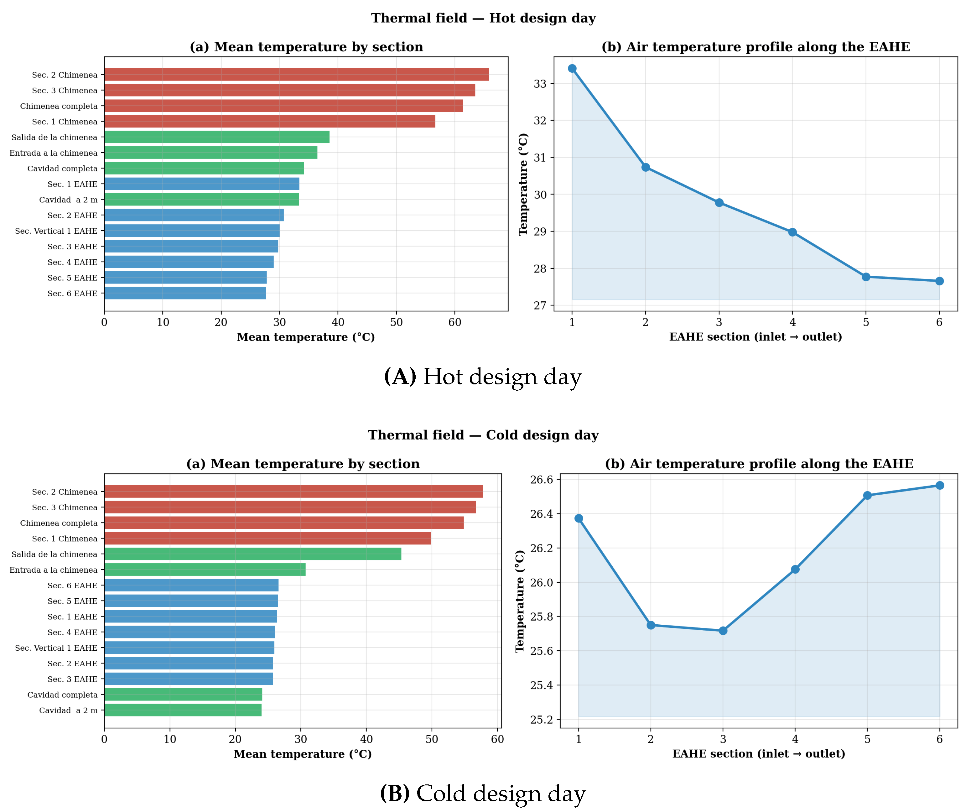
The complete system was finally evaluated for a hot and a cold representative design day. Figure 9 compares the two scenarios, and Figure 10 and Figure 11 present the detailed ventilation, energy and thermal-profile results obtained with the Python post-processing routine. The consolidated indicators are reported in

Table 8. Ventilation and thermal-energy indicators of the complete system for the hot and cold design days ($V_{\mathrm{cav}}=27$ m³, $A_{\mathrm{out}}=0.15$ m² (physical chimney outlet, $0.15\mathrm{m}\times 1\mathrm{m}$), $\rho =1.225$ kg m⁻³, $c_p=1005$ J kg⁻¹K⁻¹).

Indicator	Unit	Hot Day	Cold Day
Outlet velocity magnitude, $\overline{v}$	m s−1	0.126	0.034
Volumetric flow rate, Q	m3 h−1	67.88	18.52
Volumetric flow rate, Q	L s−1	18.86	5.15
Mass flow rate, $\dot{m}$	kg s−1	0.0231	0.0063
Air changes per hour, ACH	h−1	2.51	0.69
Renewal time	min	23.9	87.5
Solar-chimney inlet temperature	°C	36.45	30.74
Solar-chimney outlet temperature	°C	38.54	45.32
Solar-chimney $\Delta T_{\mathrm{SC}}$	°C	2.10	14.58
EAHE inlet temperature	°C	33.41	26.37
EAHE outlet temperature	°C	27.66	26.57
EAHE $\Delta T_{\mathrm{EAHE}}$	°C	$-5.75$	$+0.19$
Mean cavity temperature	°C	33.74	24.05
Solar-chimney heat gain	W	48.70	92.36
EAHE cooling power	W	133.42	1.21
Relative thermal-contribution ratio, $R_{\Delta T}$	%	273.9	1.3

.

On the hot design day, the system operates in a strong cooling regime. The EAHE cooled the air by 5.75 °C (from 33.41 °C to 27.66 °C), the solar chimney developed a driving gradient of 2.10 °C, and the buoyancy produced a volumetric flow rate of 67.88 m³ h⁻¹ (18.86 L s⁻¹), equivalent to 2.51 ACH and a renewal time of 23.9 min. The EAHE extracted 133.42 W of sensible heat from the supply air, while the chimney air gained 48.70 W from solar radiation (a driver of the flow, not a cooling contribution); the relative thermal-contribution ratio was $R_{\Delta T}=273.9\%$, confirming that the ground exchanger is the dominant thermal mechanism in hot conditions while the chimney sustains the flow. The mean cavity temperature settled at 33.74 °C (Figure 10a). On the cold design day the behavior changes qualitatively: the EAHE became almost thermally neutral, with a negligible variation of $+0.19$ °C (from 26.37 °C to 26.57 °C) because the ground and the incoming air are close to thermal equilibrium; therefore, the exchanger tempers the air without overcooling it. The solar chimney, whose glazed surface is still heated by solar radiation while the incoming air is cold, developed a much higher driving gradient of 14.58 °C, but the resulting flow was lower, 18.52 m³ h⁻¹ (5.15 L s⁻¹), equivalent to 0.69 ACH and a renewal time of 87.5 min. The mean cavity temperature settled at 24.05 °C. The reduction in ventilation rate in winter is advantageous as it limits the loss of indoor heat while still guaranteeing air renewal.

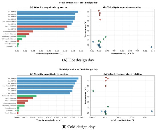
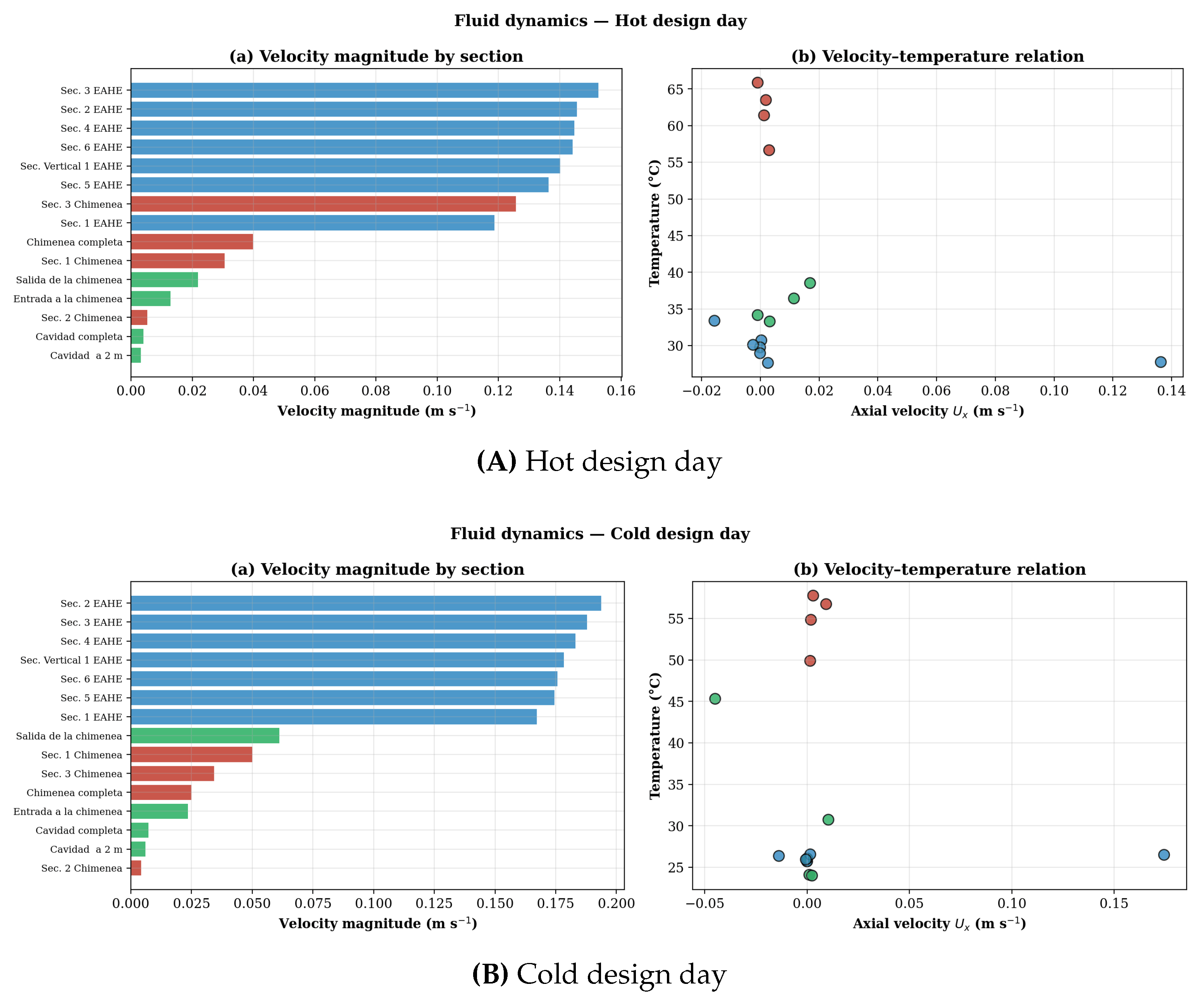
Figure 12 completes the picture with the velocity magnitude of every analyzed section and its relationship to local temperature, showing that the highest velocities concentrate in the EAHE outlet and the chimney throat in both scenarios but with a substantially larger magnitude on the hot day.

4. Discussion

The comparison of the three configurations makes it possible to separate the individual contributions of the EAHE and the solar chimney and quantify their combined effect. From a thermal point of view, the bare cavity showed the least favorable behavior: an almost uniform field at 34.42 °C and only 4.56 W of removed power. Adding EAHE reduced the mean cavity temperature to 33.45 °C and reduced the supply-air temperature by 6.81 °C, in line with the cooling potentials reported experimentally for warm–humid climates [10,11]; however, without a device to extract hot air, ventilation remained limited to 4.27 ACH. The best performance corresponded to the complete system, in which the air cooled by the EAHE is driven into the cavity, while the solar chimney generates a buoyancy force that sustains a continuous circulation. As a result, the ventilation rate reached 8.32 ACH and the removed power increased to 67.04 W.

In this work, the term “synergy” is used in a qualitative, complementary sense to describe the mutually reinforcing action of the two devices; because a solar-chimney-only configuration (without the EAHE) was not simulated, we do not claim a formally quantified synergy against an independent solar-chimney baseline. Taking the bare cavity as the baseline (2.01 ACH), the EAHE alone raises ventilation to 4.27 ACH (an increment of $+2.26$ ACH), and adding the solar chimney raises it to 8.32 ACH (a further $+4.05$ ACH). The coupled increment is therefore larger than what the EAHE contributes in isolation because the ground-cooled air increases the density contrast that drives the chimney; this mutual reinforcement—the ground-cooled air increasing the density contrast that drives the chimney—is what is here referred to as their complementary (synergistic) action. A dedicated solar-chimney-only case would be required to quantify the synergy against an independent chimney baseline. This behavior is consistent with previous CFD investigations of coupled EAHE–solar chimney systems, which reported that ground cooling improves buoyancy-driven ventilation through the complementary action of sensible heat exchange and natural convection [51].

The design-day evaluation adds a second dimension: the coupled system responds differently to contrasting climatic demands. On the hot day of design, EAHE dominates the thermal response and provides a strong 5.75 °C of air cooling, while the solar chimney maintains a ventilation of 2.51 ACH; the system behaves as an effective passive cooler. On the cold design day, the roles reverse: the EAHE becomes nearly neutral (+0.19 °C), avoiding the overcooling that would be undesirable in winter, while the naturally reduced buoyancy reduces the ventilation to 0.69 ACH, which limits the loss of indoor heat while still renewing the air. It must be stressed that this climate dependence is a passive consequence of the boundary conditions of each design day and not an active control action: no control strategy was modeled, and the term “self-adjusting” used in the previous version was removed accordingly. Similarly, the improved thermal performance reported here should be distinguished from actual thermal comfort: a mean cavity temperature of 33.2–33.7 °C on the day of the hot design represents a clear improvement over the bare cavity, but is still above the comfort range for occupied rooms; the 24.1 °C obtained on the cold day is within a comfortable range, but comfort also depends on humidity and air speed, which were not evaluated here.

To bring the hot-day cavity temperature closer to the comfort range, several measures can be derived from the present results and the literature: increasing the EAHE length or using multiple parallel ducts to raise the supply-air cooling; increasing the burial depth or the number of passes to enlarge the ground contact area; enlarging the chimney absorber area or height to increase the ACH; and combining the system with complementary passive strategies (night ventilation, shading, radiant/evaporative cooling and envelope insulation). For rooms larger than the 27 m³ cavity studied here, the relative (intensive) conclusions remain valid, but the inlet/outlet areas and the EAHE flow capacity must be scaled proportionally to the volume of the room to preserve the reported ACH.

It should be noted that the three-configuration comparison and the design-day evaluation adopt different post-processing conventions (the former uses the outlet-patch mean velocity with the Boussinesq density on the quasi-2D slice, the latter the chimney-section velocity magnitude with a fixed 27 m³ volume and constant air properties). Consequently, their absolute ventilation magnitudes are not directly interchangeable; each set of indicators is internally consistent and is interpreted within its own analysis, and unifying both under a single post-processing convention is identified as future work. The main simplifications—the steady-state assumption, the Boussinesq approximation, the quasi-two-dimensional symmetry reduction, and the prescribed wall temperatures for the design days—were adopted to keep the parametric and design day studies tractable; they represent conservative, maximum-demand scenarios. Future work should address a transient annual simulation (required before any year-round claim can be made), a fully coupled experimental validation, the reporting of $y^{+}$ and a unified post-processing convention, and the economic assessment of the system, whose viability is known to depend on regional climate and electricity tariffs [36,52].

5. Conclusions

A CFD study of an earth–air heat exchanger coupled with a solar chimney was carried out in OpenFOAM to assess the thermal and ventilation performance of a passive conditioning system for dwellings in warm–humid climates, including an evaluation for a representative hot and a representative cold design day. The main conclusions are as follows.

• Within the simulated four-day period, the soil surrounding the EAHE at a depth of 2.5 m acted as a stable thermal reservoir: the temperature of the soil adjacent to the conduit remained within a narrow range of 27.65 to 27.70 °C despite fluctuations in surface temperature. This conclusion is restricted to the simulated period; longer simulations would be required to establish seasonal or annual stability.
• Of the three configurations analyzed under identical numerical conditions, the complete system demonstrated the best overall performance, achieving an average cavity temperature of 33.20 °C, a ventilation rate of 8.32 ACH, and a cavity thermal-power extraction of 67.04 W; by comparison, the EAHE-plus-cavity configuration recorded 33.45 °C, 4.27 ACH, and 17.42 W, while the cavity alone showed 34.42 °C, 2.01 ACH, and 4.56 W. Incorporating the solar chimney increased ventilation by 94.8% relative to the EAHE-plus-cavity configuration and by 313.9% relative to the cavity alone. The ACH achieved exceeds typical residential ventilation recommendations, although a formal ASHRAE compliance assessment would require occupancy and floor-area data.
• The results indicate a complementary, mutually reinforcing interaction between the EAHE and the solar chimney: the ground-cooled air increases the density contrast that drives the chimney, so their combined operation improves air renewal and heat extraction beyond the isolated contribution of each device.
• The design-day evaluation revealed a climate-dependent response. On the hot design day, the EAHE achieved a 5.75 °C reduction in air temperature and the system maintained 2.51 ACH; on the cold design day, the EAHE became virtually thermally neutral ($+0.19$ °C), the ventilation decreased to 0.69 ACH and the cavity temperature was 24.05 $°$ C. This behavior is a passive consequence of the boundary conditions of each design day; no active control was modeled.

The coupled operation of the EAHE and the solar chimney generates a complementary, mutually reinforcing behavior that neither device achieves on its own, and its thermal and ventilation response differs markedly between the hot and cold design days analyzed. These findings provide quantitative, design-oriented criteria (burial depth, component layout, ventilation and the expected contribution of each device) for combined passive systems in warm–humid dwellings, and the open-source methodology offers a reproducible framework that can be adapted to other geometries, soils, and climates. A transient annual analysis and a fully coupled experimental validation are required to extend these design-day results to genuine year-round performance and thermal-comfort claims.

References

- International Energy Agency. Global Status Report for Buildings and Construction 2019; International Energy Agency: Paris, France, 2019. [Google Scholar]
- Pérez-Lombard, L.; Ortiz, J.; Pout, C. A review on buildings energy consumption information. Energy Build. 2008, 40, 394–398. [Google Scholar] [CrossRef] [Scilit]
- Song, Y.-l.; Darani, K.S.; Khdair, A.I.; Abu-Rumman, G.; Kalbasi, R. A review on conventional passive cooling methods applicable to arid and warm climates considering economic cost and efficiency analysis in resource-based cities. Energy Rep. 2021, 7, 2784–2820. [Google Scholar] [CrossRef] [Scilit]
- Maytorena, V.M.; Hinojosa, J.F.; Moreno, S.; Buentello-Montoya, D.A. Thermal performance analysis of a passive hybrid earth-to-air heat exchanger for cooling rooms at Mexican desert climate. Case Stud. Therm. Eng. 2023, 41, 102590. [Google Scholar] [CrossRef] [Scilit]
- Mihalakakou, G.; Souliotis, M.; Papadaki, M.; Halkos, G.; Paravantis, J.; Makridis, S.; Papaefthimiou, S. Applications of earth-to-air heat exchangers: A holistic review. Renew. Sustain. Energy Rev. 2022, 155, 111921. [Google Scholar] [CrossRef] [Scilit]
- Naja, A.; Rijal, H.B.; Zaki, S.A. A Review of Thermal Comfort in Residential Buildings: Comfort Threads and Energy Saving Potential. Energies 2022, 15, 9012. [Google Scholar] [CrossRef] [Scilit]
- Zeitoun, W.; Lin, J.; Siroux, M. A Review – Earth-air Heat Exchanger: Applications, Advances and Challenges. IOP Conf. Ser. Earth Environ. Sci. 2022, 1050, 012005. [Google Scholar] [CrossRef] [Scilit]
- Schmid, A.L.; Stanescu, G.; Errera, M.R.; Alves, A.B.M.; Da Rosa, A.R. Sizing principles and practice of an earth-air heat exchanger (EAHE) for thermal conditioning of buildings. Energy Build. 2026, 353, 116848. [Google Scholar] [CrossRef] [Scilit]
- Bughio, M.; Bahale, S.; Mahar, W.A.; Schuetze, T. Parametric Performance Analysis of the Cooling Potential of Earth-to-Air Heat Exchangers in Hot and Humid Climates. Energies 2022, 15, 7054. [Google Scholar] [CrossRef] [Scilit]
- Díaz-Hernández, H.P.; Macias-Melo, E.V.; Aguilar-Castro, K.M.; Hernández-Pérez, I.; Xamán, J.; Serrano-Arellano, J.; López-Manrique, L.M. Experimental study of an earth to air heat exchanger (EAHE) for warm humid climatic conditions. Geothermics 2020, 84, 101741. [Google Scholar] [CrossRef] [Scilit]
- Molina-Rodea, R.; Wong-Loya, J.A.; Pocasangre-Chávez, H.; Reyna-Guillén, J. Experimental evaluation of a “U” type earth-to-air heat exchanger planned for narrow installation space in warm climatic conditions. Energy Built Environ. 2024, 5, 772–786. [Google Scholar] [CrossRef] [Scilit]
- Huang, K.; Sun, Q.; Feng, G.; Zhang, L.; Li, A.; Wei, J.; Zhang, X.; Meng, X. Experimental and numerical research on the thermal performance of a vertical earth-to-air heat exchanger system. Geothermics 2025, 125, 103182. [Google Scholar] [CrossRef] [Scilit]
- Alikhani, A.; Maerefat, M.; Mohammad, S.; Sobhani, J. Analytical investigation on the optimal tube length of Earth-to-Air Heat Exchanger (EAHE). Geothermics 2025, 127, 103250. [Google Scholar] [CrossRef] [Scilit]
- Soares, T.A.; Langner, M.; Sacht, H.; Figueiredo, A.; Vicente, R. Multi-objective optimisation of an earth-to-air heat exchanger for thermal regulation in Southern Brazilian bioclimatic zones. Energy Build. 2025, 347, 116243. [Google Scholar] [CrossRef] [Scilit]
- Ali, M.H.; Alshibil, A.M.A.; Almadhhachi, M.; Machi, M.H.; Víg, P.; Farkas, I.; Kurjak, Z. Comparative modeling and performance analysis of earth-air heat exchangers in hot-arid and cold-continental climates: A case study of Baghdad and Gothenburg. Energy Convers. Manag. X 2025, 27, 101205. [Google Scholar] [CrossRef] [Scilit]
- Li, J.; Jimenez-Bescos, C.; Calautit, J.K.; Yao, J. Evaluating the energy-saving potential of earth-air heat exchanger (EAHX) for Passivhaus standard buildings in different climates in China. Energy Build. 2023, 288, 113005. [Google Scholar] [CrossRef] [Scilit]
- Torres-Ruiz, F.; Hernández-Pérez, I. Parametric study of earth-to-air heat exchanger in a hot-humid climate. J. Exp. Environ. Sci. 2023, 7, 93–110. [Google Scholar]
- Xu, Y.; Zeng, Z.; Sun, D.; Lv, H. Comparative study on thermal properties of undisturbed and compacted lateritic soils subjected to drying and wetting. Eng. Geol. 2020, 277, 105800. [Google Scholar] [CrossRef] [Scilit]
- Muñoz-Criollo, J.J.; Cleall, P.J.; Rees, S.W. Modelling thermal fluxes at the soil surface. Environ. Geotech. 2019, 6, 393–405. [Google Scholar] [CrossRef] [Scilit]
- Villar-Ramos, M.M.; Macias-Melo, E.V.; Aguilar-Castro, K.M.; Hernández-Pérez, I.; Arce, J.; Serrano-Arellano, J.; Díaz-Hernández, H.P.; López-Manrique, L.M. Parametric analysis of the thermal behavior of a single-channel solar chimney. Sol. Energy 2020, 209, 602–617. [Google Scholar] [CrossRef] [Scilit]
- Jiménez-Xamán, C.M. Estudio Térmico de una Habitación Acoplada con una Chimenea Solar. Ph.D. Thesis, Centro Nacional de Investigación y Desarrollo Tecnológico, Cuernavaca, Mexico, 2019. [Google Scholar]
- Maerefat, M.; Haghighi, A. Passive cooling of buildings by using integrated earth to air heat exchanger and solar chimney. Renew. Energy 2010, 35, 2316–2324. [Google Scholar] [CrossRef] [Scilit]
- Haghighi, A.P.; Maerefat, M. Design guideline for application of earth-to-air heat exchanger coupled with solar chimney as a natural heating system. Int. J. Low.-Carbon Technol. 2014, 10, 294–304. [Google Scholar] [CrossRef] [Scilit]
- Bai, Y.; Long, T.; Li, W.; Li, Y.; Liu, S.; Wang, Z.; Lu, J.; Huang, S. Experimental investigation of natural ventilation characteristics of a solar chimney coupled with earth-air heat exchanger (SCEAHE) system in summer and winter. Renew. Energy 2022, 193, 1001–1018. [Google Scholar] [CrossRef] [Scilit]
- Li, Y.; Long, T.; Bai, X.; Wang, L.; Li, W.; Liu, S.; Lu, J.; Huang, S. An experimental investigation on the passive ventilation and cooling performance of an integrated solar chimney and earth–air heat exchanger. Renew. Energy 2021, 175, 486–500. [Google Scholar] [CrossRef] [Scilit]
- Long, T.; Zhao, N.; Li, W.; Wei, S.; Li, Y.; Lu, J.; Qiao, Z. Numerical simulation of diurnal and annual performance of coupled solar chimney with earth-to-air heat exchanger system. Appl. Therm. Eng. 2022, 214, 118851. [Google Scholar] [CrossRef] [Scilit]
- Nguyen, V.; Nguyen, Y.; Huynh, T. Natural Ventilation and Cooling of a House with a Solar Chimney Coupled with an Earth-To-Air Heat Exchanger. In Modern Mechanics and Applications; Springer: Singapore, 2022; pp. 158–168. [Google Scholar]
- Yu, Y.; Li, H.; Niu, F.; Yu, D. Investigation of a coupled geothermal cooling system with earth tube and solar chimney. Appl. Energy 2014, 114, 209–217. [Google Scholar] [CrossRef] [Scilit]
- Serageldin, A.; Abdeen, A.; Ahmed, M.; Radwan, A.; Shmroukh, A.; Ookawara, S. Solar chimney combined with earth to-air heat exchanger for passive cooling of residential buildings in hot areas. Sol. Energy 2020, 206, 145–162. [Google Scholar] [CrossRef] [Scilit]
- Sakhri, N.; Menni, Y.; Chamkha, A.; Lorenzini, G.; Ameur, H.; Kaid, N.; Bensafi, M. Experimental study of an earth-to-air heat exchanger coupled to the solar chimney for heating and cooling applications in arid regions. J. Therm. Anal. Calorim. 2021, 145, 3349–3358. [Google Scholar] [CrossRef] [Scilit]
- Zhang, P.; Cao, D.; Hao, Z. Research on the spatial distribution of the coupled solar chimney with earth-to-air heat exchanger system performance. Therm. Sci. Eng. Prog. 2025, 60, 103368. [Google Scholar] [CrossRef] [Scilit]
- Torabipour, S.; Taheri, A.; Delfani, S.; Fayaz, R. The cooling effect of a solar chimney in combination with an earth-to-air heat exchanger in a hot and semi-desert climate. J. Therm. Anal. Calorim. 2025, 150, 14. [Google Scholar] [CrossRef] [Scilit]
- Khare, G.K.; Nikam, S.K. Assessment of the solar-coupled Earth Air Heat Exchanger (EAHE) system for sustainable residential cooling. J. Neonatal Surg. 2025, 14, 989–996. [Google Scholar]
- Pikra, G.; Darmanto, P.S.; Astina, I.M. A review of solar chimney-earth air heat exchanger (SCEAHE) system integration for thermal comfort building. J. Build. Eng. 2024, 98, 111484. [Google Scholar] [CrossRef] [Scilit]
- Mandal, D.K.; Bose, S.; Biswas, N.; Manna, N.K.; Santra, S.; Cuce, E.; Alshahrani, S. Hybrid solar chimneys: Enhancing thermal comfort and alleviating indoor air pollutants—A comprehensive review. Sol. Energy 2025, 293, 113442. [Google Scholar] [CrossRef] [Scilit]
- Koshlak, H. A Review of Earth-Air Heat Exchangers: From Fundamental Principles to Hybrid Systems with Renewable Energy Integration. Energies 2025, 18, 1017. [Google Scholar] [CrossRef] [Scilit]
- Greenshields, C.; Weller, H. OpenFOAM v12 User Guide; The OpenFOAM Foundation: London, UK, 2024; Available online: https://www.openfoam.org (accessed on 1 July 2026).
- Mateus, R.; Pereira, J.M.C.; Pinto, A. Natural ventilation of large air masses: Experimental and numerical techniques review. Energy Build. 2023, 291, 113120. [Google Scholar] [CrossRef] [Scilit]
- Sakhri, N.; Menni, Y.; Chamkha, A.J.; Lorenzini, G.; Kaid, N.; Ameur, H.; Bensafi, M. Study of heat and mass transfer through an earth to air heat exchanger equipped with fan in south west of Algeria. Int. J. Heat Technol. 2019, 37, 689–695. [Google Scholar] [CrossRef] [Scilit]
- Nel, T.O.; Pretorius, J.P.; Rousseau, P.G. Thermofluid Design and Performance Evaluation of a Natural Draft Air-Cooled Condenser Towards Annual Performance Modeling of Concentrated Solar Power Plants. Math. Comput. Appl. 2026, 31, 131. [Google Scholar] [CrossRef] [Scilit]
- Hossain, M.S.; Fayz-Al-Asad, M.; Mallik, M.S.I.; Yavuz, M.; Alim, M.A.; Khairul Basher, K.M. Numerical Study of the Effect of a Heated Cylinder on Natural Convection in a Square Cavity in the Presence of a Magnetic Field. Math. Comput. Appl. 2022, 27, 58. [Google Scholar] [CrossRef] [Scilit]
- Yao, J.; Rezaeiravesh, S.; Schlatter, P.; Hussain, F. Direct numerical simulations of turbulent pipe flow up to Reτ≈5200. J. Fluid Mech. 2023, 956, A18. [Google Scholar] [CrossRef] [Scilit]
- Balabanov, R.; Usov, L.; Troshin, A.; Vlasenko, V.; Sabelnikov, V. A Differential Subgrid Stress Model and Its Assessment in Large Eddy Simulations of Non-Premixed Turbulent Combustion. Appl. Sci. 2022, 12, 8491. [Google Scholar] [CrossRef] [Scilit]
- Joo, D.-S. A global similarity correction for the RANS modeling of natural convection in unstably stratified flows. arXiv 2025, arXiv:2501.12973. [Google Scholar]
- Hafez, K.; Elsamni, O.; Zakaria, K. Numerical investigation of the fully developed turbulent flow over a moving wavy wall using k–ε turbulence model. Alex. Eng. J. 2011, 50, 145–162. [Google Scholar] [CrossRef] [Scilit]
- Bragg, A.D.; de Bruyn Kops, S.M. Understanding the effect of Prandtl number on momentum and scalar mixing rates in neutral and stably stratified flows using gradient field dynamics. J. Fluid Mech. 2024, 992, A5. [Google Scholar] [CrossRef] [Scilit]
- Hemanth, V.; Kushal, K.S.; Varun, S.S. Aerodynamic Study on Low Reynolds Number Aerofoil. ACS J. Sci. Eng. 2024, 4, 39–57. [Google Scholar] [CrossRef] [Scilit]
- Cheng, J.; Xu, H.; Tang, Z.; Zhou, P. Study on single-phase and two-phase flow and heat transfer characteristics of HFE-7100 in manifold microchannel heat sink with corrugated bottom. Therm. Sci. 2024, 28, 1819–1836. [Google Scholar] [CrossRef] [Scilit]
- Saroja, G.; Rianto, S.; Abdurrouf; Sakti, S.P.; Nurhuda, M. Stretched Meshing in a 2D Computational Domain with Elbow Edges for CFD Applications. J. Adv. Res. Fluid Mech. Therm. Sci. 2024, 116, 41–50. [Google Scholar] [CrossRef] [Scilit]
- Torres-Aguilar, C.; Moreno-Bernal, P.; Nesmachnow, S.; Rossit, D. A parallel multi-threading global energy balance for a room thermal analysis in an unsteady state. In High Performance Computing. CARLA 2024; Communications in Computer and Information Science; Springer: Cham, Switzerland, 2025; Volume 2270. [Google Scholar]
- Zamora, B.; Gutiérrez-Romero, J.E. Numerical Analysis of the Impact of Incoming Cold Airstream on a Room Shaped to Passive Solar Chimney Coupled with Earth-Air Heat Exchanger. Processes 2026, 14, 796. [Google Scholar] [CrossRef] [Scilit]
- Patin, M.; Rousse, D.R. Optimizing economic performances of foundation earth-to-air heat exchangers for low-technology residential air-conditioning. Energy Build. 2025, 328, 115250. [Google Scholar] [CrossRef] [Scilit]
Disclaimer/Publisher’s Note: The statements, opinions and data contained in all publications are solely those of the individual author(s) and contributor(s) and not of MDPI and/or the editor(s). MDPI and/or the editor(s) disclaim responsibility for any injury to people or property resulting from any ideas, methods, instructions or products referred to in the content. |
© 2026 by the authors. Licensee MDPI, Basel, Switzerland. This article is an open access article distributed under the terms and conditions of the Creative Commons Attribution (CC BY) license.