Accurate Treatment of Solution and Flux Discontinuities in 2D Time-Dependent Interface Problems via Meshless Method

Abstract

Interface problems frequently arise in applications including heat conduction with composite materials, fluid flow in porous media, and diffusion–reaction processes across heterogeneous domains. This paper presents a numerical method that combines radial basis functions with a finite difference method to solve two-dimensional linear and nonlinear parabolic-type interface problems. In the proposed approach, spatial derivatives are approximated using multi-quadric radial basis functions, while the time derivative is discretized via a finite difference method. The method is applied to both linear and nonlinear problems. Gaussian elimination is used to solve the resulting algebraic equation in linear cases, while a quasi-Newton linearization technique is used to handle the nonlinear terms in nonlinear cases. Several numerical experiments are performed to assess the performance of the proposed method. The results are compared with the Haar wavelet collocation method, demonstrating the improved accuracy, computational efficiency, and straightforward implementation of the method.

1. Introduction

Many physical phenomena take place within domains divided into multiple regions, each possessing distinct physical or mathematical properties. Interfaces appear in situations like fluid or composite material flows. Classical examples include heat transfer through layered rods or wave propagation in non-uniform media, which reflect parabolic and hyperbolic partial differential equation (PDE) behaviors, respectively. In one-dimensional domains, an interface is the common border between two intervals, and in higher-dimensional domains, it is the common border between two regions. Accurate modeling of such interfaces is essential in various applications such as crystal formation, wave transmission, cardiac blood flow, material design, fluid transport, fracture dynamics, and biological systems [1,2].

Parabolic PDEs describe time-dependent phenomena and are commonly used in modeling processes like heat conduction, diffusion of particles, underwater acoustics, and financial instrument pricing [3]. A classical example is the diffusion equation, which can be adapted to capture phenomena involving momentum, mass and energy transfer. Over the past two decades, significant research has focused on developing efficient numerical techniques to approximate the solutions of such equations. These methods are typically translated into computer algorithms and implemented via software to produce numerical results. Among the most established approaches are the finite volume method, finite element method, finite difference method (FDM) and Fourier spectral techniques.

Several researchers have focused on the numerical solution of parabolic PDEs due to their practical significance. Haider et al. applied meshless and multi collocation methods to numerically solve parabolic interface problems (PIPs) [4]. A spatially second-order alternating directional implicit technique for solving three-dimensional PIPs was proposed by Z. Wei et al. in [5]. Using a linearized backward Euler method, Shi and Wang used the Galerkin finite element approach to solve nonlinear parabolic equations [6]. Using the finite element tearing and interconnecting-based domain decomposition method, Benes and Kruis suggested and studied an algorithm with multiple time steps for nonlinear parabolic problems [7]. Some of the recent work on interface problems can be found in [8,9,10,11,12,13,14,15,16,17,18].

Among advanced numerical techniques, meshless methods stand out for their capability to handle irregular domains and scattered data cases where traditional mesh-based methods struggle. These methods are particularly well-suited for problems with intricate geometries or interfaces characterized by discontinuities in the solution or its gradient. Despite their potential, research into robust and accurate meshless techniques for general interface problems remains relatively limited.

Meshless techniques are gaining momentum due to their flexibility, ease of extension to complex geometries, and independence from structured meshes. Unlike conventional methods that rely on predefined grids or elements for spatial discretization, meshless approaches generate systems of algebraic equations over the domain using scattered or uniformly distributed nodes. This makes them advantageous in situations where mesh generation is difficult or computationally expensive.

Several meshless methods have been proposed for solving PDEs. Notable among them are the meshless local Petrov–Galerkin method [19,20], the method of fundamental solutions [21,22,23,24], the singular boundary method [25,26], and the boundary knot method [27,28]. A particularly promising category within meshless approaches is radial basis function (RBF)-based collocation techniques [29,30,31,32,33]. For example, Shin et al. applied a meshless collocation approach to one-dimensional elliptic interface equations [34], while Jamil et al. extended this to two-dimensional $\left(2D\right)$ steady-state problems involving heterogeneous conduction and bioheat transfer [35]. Other studies have applied RBFs to solve linearized Poisson–Boltzmann, Poisson, and bioheat equations under interface constraints [30]. Moreover, Martin et al. explored RBF methods for solving the $2D$ elastic wave equation [36], and later applied an RBF-generated finite difference scheme to analyze heat equilibrium problems with smoothly varying interfaces [37]. Recent studies have used meshfree RBFs and Residual Power Series methods to solve fractional-order mathematical models [38,39,40].

In this study, we introduce a new hybrid technique that combines RBF with FDM to numerically solve $2D$ linear and nonlinear parabolic problems using single interfaces. The equations are defined below:

$$w_{\mathtt{t}}=\nabla ·(\beta \nabla w)+\varphi ,\mathtt{t}\ge {\mathtt{t}}_0,(\zeta ,\eta )\in \Omega ,$$

(1)

and the nonlinear problem will be of the form:

$$w_{\mathtt{t}}=\nabla ·(\beta \nabla w)+N\left(w\right)+\varphi ,\mathtt{t}\ge {\mathtt{t}}_0,(\zeta ,\eta )\in \Omega ,$$

(2)

such that ${\Omega }_1=[-1,\alpha ]\times [-1,1]$ and ${\Omega }_2=[\alpha ,1]\times [-1,1]$ are the subdomains of $\Omega =[-1,1]\times [-1,1]$. $w=w(\zeta ,\mathtt{t})$ is the unknown function, while $\varphi =\varphi (\zeta ,t)$ is the source function and the coefficient $\beta =\beta \left(\zeta \right)$, where $\zeta =(\zeta ,\eta )\in \Omega \subset R^2$, and $\nabla =({\displaystyle \frac{\partial }{{\partial }_{\zeta }}},{\displaystyle \frac{\partial }{{\partial }_{\eta }}})$. The function mentioned is

$$\left(k(\zeta ,\eta ,\mathtt{t}),w(\zeta ,\eta ,\mathtt{t}),f(\zeta ,\eta ,\mathtt{t})\right)=\left\{\begin{array}{cc}\left(k_1(\zeta ,\eta ,\mathtt{t}),w_1(\zeta ,\eta ,\mathtt{t}),f_1(\zeta ,\eta ,\mathtt{t})\right),\hfill & \mathrm{for}(\zeta ,\eta )\in {\Omega }_1,\hfill \\ \left(k_2(\zeta ,\eta ,\mathtt{t}),w_2(\zeta ,\eta ,\mathtt{t}),f_2(\zeta ,\eta ,\mathtt{t})\right),\hfill & \mathrm{for}(\zeta ,\eta )\in {\Omega }_2.\hfill \end{array}\right.$$

The initial condition is: $w(\zeta ,\eta ,0)=w_0(\zeta ,\eta )$.

The Dirichlet boundary conditions (BCs) are given by

$$\begin{array}{cccccc}\hfill w(-1,\eta ,\mathtt{t})& ={\delta }_1(-1,\eta ,\mathtt{t}),\hfill & \hfill w(1,\eta ,\mathtt{t})& ={\delta }_2(1,\eta ,\mathtt{t}),\hfill & \hfill & -1\le \eta \le 1,\hfill \\ \hfill w(\zeta ,-1,\mathtt{t})& ={\delta }_1(\zeta ,-1,\mathtt{t}),\hfill & \hfill w(\zeta ,1,\mathtt{t})& ={\delta }_2(\zeta ,1,\mathtt{t}),\hfill & \hfill & -1\le \zeta \le 0,\hfill \\ \hfill w(\zeta ,-1,\mathtt{t})& ={\delta }_2(\zeta ,-1,\mathtt{t}),\hfill & \hfill w(\zeta ,1,\mathtt{t})& ={\delta }_2(\zeta ,1,\mathtt{t}),\hfill & \hfill & 0\le \zeta \le 1.\hfill \end{array}$$

whereas, at the interface point $\zeta =\alpha$, the following interface conditions will be considered:

$$w_2(\alpha ,\eta ,\mathtt{t})-w_1(\alpha ,\eta ,\mathtt{t})={\mu }_1,$$

(3)

$$k_2(\alpha ,\eta ,\mathtt{t})w_{2\zeta }(\alpha ,\eta ,\mathtt{t})-k_1(\alpha ,\eta ,\mathtt{t})w_{1\zeta }(\alpha ,\eta ,\mathtt{t})={\mu }_2.$$

(4)

The functions $f_1(\zeta ,\eta ,\mathtt{t}),f_2(\zeta ,\eta ,\mathtt{t}),{\kappa }_1(\zeta ,\eta ,\mathtt{t})>0,{\kappa }_2(\zeta ,\eta ,\mathtt{t})>0$ are smooth functions defined in corresponding subregions of $\Omega$.

The Main Purpose of This Study

In this study, the main objective is to create a reliable and accurate numerical method for solving $2D$ parabolic PDEs using both variable and constant coefficients. The proposed approach combines the meshless collocation method (MCM) with the FDM, utilizing the strengths of each technique. In this hybrid formulation, temporal derivatives are discretized using FDM, while spatial derivatives are handled through MCM, which leverages RBFs for high accuracy and flexibility in complex geometries. To address nonlinearities in the governing equations, the nonlinear terms are linearized using the quasi-Newton linearization technique (QNLT). This method offers a significant computational advantage over the traditional Newton method by eliminating the need for repeated computation of the Jacobian matrix at each iteration. Additionally, QNLT effectively captures the dynamic behavior of nonlinear wave structures, including solitons, making it a suitable choice for nonlinear diffusion-type problems. The numerical results demonstrate that the proposed method is stable and efficient.

The structure of the paper is as follows: RBFs and their characteristics are given in Section 2. The combination of the MCM-FDM formulation and the construction of the numerical method is covered in detail in Section 3. In Section 4, a couple of numerical experiments are provided that confirm the precision and effectiveness of the methodology. Finally, Section 5 offers concluding remarks and highlights key findings of the study.

2. Radial Basis Functions

If there is a function of one variable, then a function $\psi :{\mathbb{R}}^d\to \mathbb{R}$ is called radial: $[0,\infty )\to \mathbb{R}$ so that $\psi \left(\zeta \right)=\varphi \left(\zeta \right)$; in this case, $d\in \mathbb{N}$, and the Euclidean norm $\parallel ·\parallel$ is utilized. The value of $\psi \left(r\right)$, a univariate continuous real valued RBF, is determined by the distance measured from the origin or any fixed center point [41]. In this work, we focus on multi-quadric (MQ) RBF as the foundation for developing meshless numerical solutions for interface problems. The MQ RBF is one of the earliest and most extensively studied forms, originally introduced by Hardy for scattered data interpolation [42].The MQ function is defined as

$$\psi \left(r\right)=\sqrt{r^2+c^2}.$$

(5)

where $r=\parallel \zeta -{\zeta }_i\parallel$ is the Euclidean distance between a point $\zeta$ and a center ${\zeta }_i$, and $c>0$ is a shape parameter that influences the flatness or peakedness of the basis function. The MCM, when combined with RBFs like MQ, has been successfully applied to a wide range of ordinary and PDEs. However, like all numerical techniques, it has limitations. Although MCM yields accurate results with a moderate number of collocation points, its performance may degrade as the number of points increases. It is worth noting that the conditioning difficulties often reported for MQ-RBF interpolation matrices are primarily associated with finite-precision arithmetic rather than an inherent limitation of the MQ-RBF method itself. Similar behavior is observed for classical Hilbert and Vandermonde matrices, which may appear numerically singular in standard double-precision computations but can still provide highly accurate solutions when higher-precision arithmetic is employed. Therefore, the reported ill-conditioning should be interpreted as a numerical implementation issue rather than a deficiency of the underlying approximation scheme. Furthermore, in this study, a constant MQ shape parameter was used throughout the computational domain. Its value was selected empirically through numerical experimentation to achieve a satisfactory balance between accuracy and stability. Although variable shape parameter strategies have been shown to improve the accuracy and conditioning in some applications, the investigation of optimal shape parameter selection is beyond the scope of the present work and remains an interesting direction for future research. These observations provide practical guidance for selecting the shape parameter c, and detailed discussions on its effects are available in the literature [43,44]. It is well known that MQ-RBF approximations may exhibit ill-conditioning as the number of nodes increases or when unsuitable shape parameter values are employed. In the present study, this issue was controlled through careful selection of the shape parameter and node distribution. Furthermore, condition number analysis confirms that the resulting system matrices remain reasonably well-conditioned for the considered discretizations, leading to stable and accurate numerical solutions.

3. Construction of the Numerical Method

In the present study, the collocation nodes are distributed uniformly over the computational domain $\Omega =[-1,1]\times [-1,1]$. The domain is divided into two subdomains ${\Omega }_1$ and ${\Omega }_2$ separated by the interface $\zeta =\alpha$. In each subdomain, a structured grid of nodes is generated such that ${\zeta }_i=-1+i\Delta \zeta$ and ${\eta }_j=-1+j\Delta \eta$, where $\Delta \zeta$ and $\Delta \eta$ denote the uniform spatial step sizes in the $\zeta$ and $\eta$ directions, respectively. The collocation points include interior nodes, boundary nodes, and interface nodes. Special care is taken to place nodes exactly on the interface $\zeta =\alpha$ to accurately enforce the interface conditions. The total number of nodes is denoted by N, and the nodes are distributed evenly in both subdomains to maintain numerical stability and accuracy.

In order to calculate the unknown function $w(\zeta ,\eta ,\mathtt{t})$, we employ the MQ RBFs. To handle the time-dependent component, the temporal derivative is discretized using the first-order forward difference scheme as follows:

$$w_{\mathtt{t}}={\displaystyle \frac{w(\zeta ,\eta ,\mathtt{t})-w(\zeta ,\eta ,{\mathtt{t}}_0)}{\Delta \mathtt{t}}}$$

(6)

where $\mathtt{t}={\mathtt{t}}_0+\Delta \mathtt{t}$, and the time-step size is $\Delta \mathtt{t}$. The initial time is denoted by ${\mathtt{t}}_0$, while t is the final time-step. In the spatial domain, the solution in each subdomain is approximated using MQ RBFs. For the subdomain ${\Omega }_1$, the function $w_1(\zeta ,\eta )$ is represented as

$$w_1(\zeta ,\eta )={\displaystyle \sum _{i=1}^{M_1+1}}{\lambda }_i\left(\mathtt{t}\right)\varphi \left({∥(\zeta ,\eta )-({\zeta }_i,{\eta }_i)∥}_2\right),(\zeta ,\eta )\in {\Omega }_1,$$

(7)

and similarly, the function $w_2(\zeta ,\eta )$ over ${\Omega }_2$ is expressed as

$$w_2(\zeta ,\eta )={\displaystyle \sum _{i=M_1+1}^N}{\gamma }_i\left(\mathtt{t}\right)\varphi \left({∥(\zeta ,\eta )-({\zeta }_i,{\eta }_i)∥}_2\right),(\zeta ,\eta )\in {\Omega }_2,$$

(8)

where

$$\varphi \left({∥(\zeta ,\eta )-({\zeta }_i,{\eta }_i)∥}_2\right)=\sqrt{1+{\left(ϵ{∥(\zeta ,\eta )-({\zeta }_i,{\eta }_i)∥}_2\right)}^2}.$$

At $\zeta =-1,1$, the boundary approximation using Equations (7) and (8) become

$${\displaystyle \sum _{i=1}^{M_1+1}}{\lambda }_i\left(\mathtt{t}\right)\varphi \left({∥(-1,\eta )-({\zeta }_i,{\eta }_i)∥}_2\right)={\delta }_1\left(\mathtt{t}\right),$$

(9)

$${\displaystyle \sum _{i=M_1+1}^N}{\gamma }_i\left(\mathtt{t}\right)\varphi \left({∥(1,\eta )-({\zeta }_i,{\eta }_i)∥}_2\right)={\delta }_2\left(\mathtt{t}\right),$$

(10)

where ${\delta }_1\left(\mathtt{t}\right)=w(-1,\eta ,\mathtt{t})$, and ${\delta }_2\left(\mathtt{t}\right)=w(1,\eta ,\mathtt{t})$.

At the interface $\zeta =\alpha$, the continuity of the function and its flux lead to

$${\displaystyle \sum _{i=M_1+1}^N}{\gamma }_i\left(\mathtt{t}\right)\varphi \left(\parallel (\alpha ,\eta )-({\zeta }_i,{\eta }_i){\parallel }_2\right)-{\displaystyle \sum _{i=1}^{M_1+1}}{\lambda }_i\left(\mathtt{t}\right)\varphi \left(\parallel (\alpha ,\eta )-({\zeta }_i,{\eta }_i){\parallel }_2\right)={\mu }_1({\eta }_k,\mathtt{t}),$$

(11)

$$k_2{\displaystyle \sum _{i=M_1+1}^N}{\gamma }_i\left(\mathtt{t}\right)\varphi \left(\parallel (\alpha ,\eta )-({\zeta }_i,{\eta }_i){\parallel }_2\right)-k_1{\displaystyle \sum _{i=1}^{M_1+1}}{\lambda }_i\left(\mathtt{t}\right)\varphi \left(\parallel (\alpha ,\eta )-({\zeta }_i,{\eta }_i){\parallel }_2\right)={\mu }_2({\eta }_k,\mathtt{t}).$$

(12)

The time derivative is approximated using the forward FDM. Thus, Equation (1) become

$$w(\zeta ,\eta ,\mathtt{t})-\Delta \mathtt{t}{\left(k(\zeta ,\eta )w_{\zeta }(\zeta ,\eta ,\mathtt{t})\right)}_{\zeta }-\Delta \mathtt{t}{\left(k(\zeta ,\eta )w_{\eta }(\zeta ,\eta ,\mathtt{t})\right)}_{\eta }=w(\zeta ,\eta ,{\mathtt{t}}_0)+\Delta \mathtt{t}f(\zeta ,\eta ,\mathtt{t}).$$

(13)

The linear and nonlinear cases of the preceding systems will be addressed separately.

3.1. Linear Case

In the linear scenario, substituting the MQ RBF expansions and their derivatives into the above Equation (13) results in the following system of algebraic equations for the subdomains ${\Omega }_1$ and ${\Omega }_2$.

$$\begin{array}{cc}\hfill & {\displaystyle \sum _{i=1}^{M_1+1}}{\lambda }_i\left(\mathtt{t}\right)\varphi \left(\parallel (\zeta ,\eta )-({\zeta }_i,{\eta }_i){\parallel }_2\right)-\Delta \mathtt{t}{k}_1(\zeta ,\eta ){\displaystyle \sum _{i=1}^{M_1+1}}{\lambda }_i\left(\mathtt{t}\right){\varphi }_{\zeta \zeta }\left(\parallel (\zeta ,\eta )-({\zeta }_i,{\eta }_i){\parallel }_2\right)\hfill \\ \hfill & -\Delta \mathtt{t}{k}_{1\zeta }(\zeta ,\eta ){\displaystyle \sum _{i=1}^{M_1+1}}{\lambda }_i\left(\mathtt{t}\right){\varphi }_{\zeta }\left(\parallel (\zeta ,\eta )-({\zeta }_i,{\eta }_i){\parallel }_2\right)-\Delta \mathtt{t}{k}_1(\zeta ,\eta ){\displaystyle \sum _{i=1}^{M_1+1}}{\lambda }_i\left(\mathtt{t}\right){\varphi }_{\eta \eta }\left(\parallel (\zeta ,\eta )-({\zeta }_i,{\eta }_i){\parallel }_2\right)\hfill \\ \hfill & -\Delta \mathtt{t}{k}_{1\eta }(\zeta ,\eta ){\displaystyle \sum _{i=1}^{M_1+1}}{\lambda }_i\left(\mathtt{t}\right){\varphi }_{\eta }\left(\parallel (\zeta ,\eta )-({\zeta }_i,{\eta }_i){\parallel }_2\right)=w(\zeta ,\eta ,{\mathtt{t}}_0)+\Delta \mathtt{t}{f}_1(\zeta ,\eta ,\mathtt{t}),(\zeta ,\eta )\in {\Omega }_1,\hfill \end{array}$$

(14)

$$\begin{array}{cc}\hfill & {\displaystyle \sum _{i=M_1+1}^N}{\gamma }_i\left(\mathtt{t}\right)\varphi \left(\parallel (\zeta ,\eta )-({\zeta }_i,{\eta }_i){\parallel }_2\right)-\Delta \mathtt{t}{k}_2(\zeta ,\eta ){\displaystyle \sum _{i=M_1+1}^N}{\gamma }_i\left(\mathtt{t}\right){\varphi }_{\zeta \zeta }\left(\parallel (\zeta ,\eta )-({\zeta }_i,{\eta }_i){\parallel }_2\right)\hfill \\ \hfill & -\Delta \mathtt{t}{k}_{2\zeta }(\zeta ,\eta ){\displaystyle \sum _{i=M_1+1}^N}{\gamma }_i\left(\mathtt{t}\right){\varphi }_{\zeta }\left(\parallel (\zeta ,\eta )-({\zeta }_i,{\eta }_i){\parallel }_2\right)-\Delta \mathtt{t}{k}_2(\zeta ,\eta ){\displaystyle \sum _{i=M_1+1}^N}{\gamma }_i\left(\mathtt{t}\right){\varphi }_{\eta \eta }\left(\parallel (\zeta ,\eta )-({\zeta }_i,{\eta }_i){\parallel }_2\right)\hfill \\ \hfill & -\Delta \mathtt{t}{k}_{2\eta }(\zeta ,\eta ){\displaystyle \sum _{i=M_1+1}^N}{\gamma }_i\left(\mathtt{t}\right){\varphi }_{\eta }\left(\parallel (\zeta ,\eta )-({\zeta }_i,{\eta }_i){\parallel }_2\right)=w(\zeta ,\eta ,{\mathtt{t}}_0)+\Delta \mathtt{t}{f}_2(\zeta ,\eta ,\mathtt{t}),(\zeta ,\eta )\in {\Omega }_2.\hfill \end{array}$$

(15)

Discretization produces the following equation system.

$$\begin{array}{cc}\hfill & {\displaystyle \sum _{i=1}^{M_1+1}}{\lambda }_i\left(\mathtt{t}\right)\varphi \left(\parallel ({\zeta }_j,{\eta }_j)-({\zeta }_i,{\eta }_i){\parallel }_2\right)-\Delta \mathtt{t}{k}_1({\zeta }_j,{\eta }_j){\displaystyle \sum _{i=1}^{M_1+1}}{\lambda }_i\left(\mathtt{t}\right){\varphi }_{\zeta \zeta }\left(\parallel ({\zeta }_j,{\eta }_j)-({\zeta }_i,{\eta }_i){\parallel }_2\right)\hfill \\ \hfill & -\Delta \mathtt{t}{k}_{1\zeta }({\zeta }_j,{\eta }_j){\displaystyle \sum _{i=1}^{M_1+1}}{\lambda }_i\left(\mathtt{t}\right){\varphi }_{\zeta }\left(\parallel ({\zeta }_j,{\eta }_j)-({\zeta }_i,{\eta }_i){\parallel }_2\right)-\Delta \mathtt{t}{k}_1({\zeta }_j,{\eta }_j){\displaystyle \sum _{i=1}^{M_1+1}}{\lambda }_i\left(\mathtt{t}\right){\varphi }_{\eta \eta }\left(\parallel ({\zeta }_j,{\eta }_j)-({\zeta }_i,{\eta }_i){\parallel }_2\right)\hfill \\ \hfill & -\Delta \mathtt{t}{k}_{1\eta }({\zeta }_j,{\eta }_j){\displaystyle \sum _{i=1}^{M_1+1}}{\lambda }_i\left(\mathtt{t}\right){\varphi }_{\eta }\left(\parallel ({\zeta }_j,{\eta }_j)-({\zeta }_i,{\eta }_i){\parallel }_2\right)\hfill \\ \hfill & =w({\zeta }_j,{\eta }_j,{\mathtt{t}}_0)+\Delta \mathtt{t}{f}_1({\zeta }_j,{\eta }_j,\mathtt{t}),j=2,\dots ,M_1,\hfill \end{array}$$

(16)

$$\begin{array}{cc}\hfill & {\displaystyle \sum _{i=M_1+1}^N}{\gamma }_i\left(\mathtt{t}\right)\varphi \left(\parallel ({\zeta }_j,{\eta }_j)-({\zeta }_i,{\eta }_i){\parallel }_2\right)-\Delta \mathtt{t}{k}_2({\zeta }_j,{\eta }_j){\displaystyle \sum _{i=M_1+1}^N}{\gamma }_i\left(\mathtt{t}\right){\varphi }_{\zeta \zeta }\left(\parallel ({\zeta }_j,{\eta }_j)-({\zeta }_i,{\eta }_i){\parallel }_2\right)\hfill \\ \hfill & -\Delta \mathtt{t}{k}_{2\zeta }({\zeta }_j,{\eta }_j){\displaystyle \sum _{i=M_1+1}^N}{\gamma }_i\left(\mathtt{t}\right){\varphi }_{\zeta }\left(\parallel ({\zeta }_j,{\eta }_j)-({\zeta }_i,{\eta }_i){\parallel }_2\right)-\Delta \mathtt{t}{k}_2({\zeta }_j,{\eta }_j){\displaystyle \sum _{i=M_1+1}^N}{\gamma }_i\left(\mathtt{t}\right){\varphi }_{\eta \eta }\left(\parallel ({\zeta }_j,{\eta }_j)-({\zeta }_i,{\eta }_i){\parallel }_2\right)\hfill \\ \hfill & -\Delta \mathtt{t}{k}_{2\eta }({\zeta }_j,{\eta }_j){\displaystyle \sum _{i=M_1+1}^N}{\gamma }_i\left(\mathtt{t}\right){\varphi }_{\eta }\left(\parallel ({\zeta }_j,{\eta }_j)-({\zeta }_i,{\eta }_i){\parallel }_2\right)\hfill \\ \hfill & =w({\zeta }_j,{\eta }_j,{\mathtt{t}}_0)+\Delta \mathtt{t}{f}_2({\zeta }_j,{\eta }_j,\mathtt{t}),j=M_1+2,\dots ,N-1.\hfill \end{array}$$

(17)

Equations (16) and (17) together with Equations (9)–(12) form a linear system of $N+1$ equations along with $N+1$ unknowns: ${\lambda }_i\left(t\right),i=1,2,3,\dots ,M_1+1$ and ${\gamma }_i\left(t\right),i=M_1+1,M_1+2,\dots ,N$. The discretized system can then be written in the matrix form:

$$\mathbf{SQ}=\mathbf{P},$$

(18)

The following equation is used to find the unknown expansion coefficients in $\mathbf{Q}$:

$$\mathbf{Q}={\mathbf{S}}^{-1}\mathbf{P}.$$

(19)

In the end, the approximate solution is derived by inserting the obtained expansion coefficients into Equations (7) and (8).

3.2. Nonlinear Case

Consider the nonlinear problem

$$w_{\mathtt{t}}=\nabla ·(\beta \nabla w)+N\left(w\right)+\varphi ,\mathtt{t}\ge {\mathtt{t}}_0,(\zeta ,\eta )\in \Omega ,$$

(20)

where $N\left(w\right)$ denotes the nonlinear operator. In the present work, the nonlinear term is taken as

$$N\left(w\right)=w{w}_{\zeta }.$$

(21)

To avoid solving the nonlinear system directly, the quasi-Newton linearization technique is employed. Let $w^n$ be the known solution at the current iteration and $w^{n+1}$ be the unknown solution at the next iteration. Using the quasi-Newton approximation, the nonlinear term is linearized as

$${\left(w{w}_{\zeta }\right)}^{n+1}=w^n{\left(w_{\zeta }\right)}^{n+1}+w^{n+1}{\left(w_{\zeta }\right)}^n-w^n{\left(w_{\zeta }\right)}^n.$$

(22)

Substituting Equation (22) into Equation (20) gives

$$w_{\mathtt{t}}^{n+1}=\nabla ·\left(\beta \nabla w^{n+1}\right)+w^n{\left(w_{\zeta }\right)}^{n+1}+w^{n+1}{\left(w_{\zeta }\right)}^n-w^n{\left(w_{\zeta }\right)}^n+\varphi .$$

(23)

Equation (23) is linear with respect to the unknown solution $w^{n+1}$, while all nonlinear coefficients are evaluated using the previously computed solution $w^n$. Consequently, only a linear system is solved at each quasi-Newton iteration.

The iterative procedure is continued until the relative difference between two successive approximations satisfies a prescribed convergence tolerance. The stopping criterion is defined as

$${\displaystyle \frac{{∥w^{n+1}-w^n∥}_{\infty }}{{∥w^{n+1}∥}_{\infty }}}<\epsilon ,$$

(24)

where ${\parallel ·\parallel }_{\infty }$ denotes the maximum norm, and $\epsilon$ is the prescribed convergence tolerance. Throughout this work, the tolerance is taken as

$$\epsilon ={10}^{-6}.$$

(25)

If the convergence criterion in Equation (24) is satisfied, the iterative process is terminated. Otherwise, the computed solution $w^{n+1}$ is taken as the updated approximation, and the quasi-Newton linearization is repeated until the prescribed tolerance is achieved.

4. Stability Analysis

To evaluate the stability of MCM, it is necessary to examine the condition number of the resulting algebraic system, as a well-conditioned system is a key indicator of numerical stability [45]. In the proposed method, the discretization process leads to a system of linear equations of the form

$$SQ=P,$$

where S denotes the coefficient matrix constructed from RBF approximations at the collocation nodes, Q is the vector of unknown coefficients, and P represents the load vector determined by the governing equation and the boundary/interface conditions.

Definition 1

(See [46]). A numerical method that produces a sequence of algebraic systems of the form $SQ=P$ is considered stable if the inverse of the coefficient matrix $S^{-1}$ exists for all sufficiently large numbers of collocation nodes ($N>N_0$), and if there exists a constant C, independent of N, such that

$$\parallel S^{-1}\parallel \le C\forall N>N_0.$$

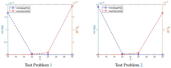
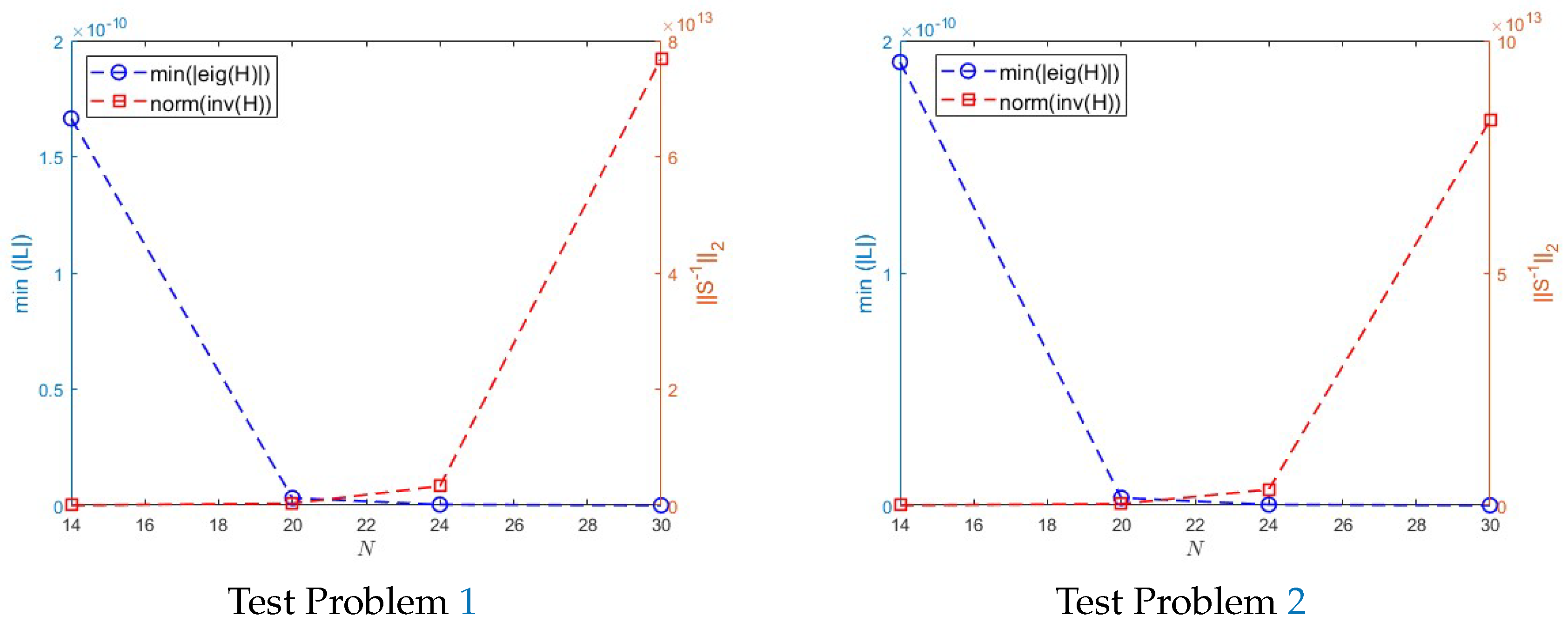
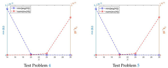
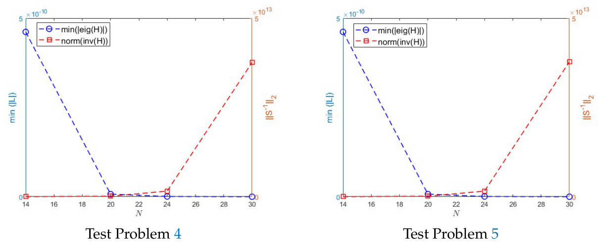
Since the eigenvalues of $S^{-1}$ are the reciprocals of those of S (denoted by $\lambda$), stability can be assessed by examining the eigenvalues of S. For a numerically stable method, these eigenvalues must remain bounded away from zero as $N\to \infty$. Accordingly, we compute the minimum eigenvalue magnitude, $min\left|\lambda \right|$, for both the linear and nonlinear benchmark problems. The results in Figure 1 and Figure 2 demonstrate that increasing the number of collocation nodes N does not lead to a significant growth in $\parallel S^{-1}{\parallel }_2$. These findings confirm that the proposed MCM framework is numerically stable.

Figure 1. The stability analysis of the proposed method for linear test problems at $N=30$, $\Delta t=0.05$, $t=1$, $a=-1$ and $b=1$.

Figure 2. A stability analysis of the proposed method for nonlinear test problems is conducted at $N=30$, $\Delta t=0.05$, and $t=1$, within the computational domain $[a,b]=[-1,1]$.

Temporal Discretization and Fully Discrete Stability

For time integration, the Forward Euler method is employed due to its simplicity and computational efficiency. The fully discrete scheme can be written as

$$w^{n+1}=w^n+\Delta t(S{w}^n+F^n).$$

It is well known that the Forward Euler method is conditionally stable. Therefore, the stability of the fully discrete scheme requires the time step $\Delta t$ to satisfy a suitable restriction of the form

$$\Delta t\rho \left(S\right)\le \gamma ,$$

where $\rho \left(S\right)$ denotes the spectral radius of the spatial operator, and $\gamma$ is a constant depending on the problem structure.

In all numerical experiments reported in this work, the time step $\Delta t$ is carefully selected to satisfy this stability condition. Numerical tests confirm that a further reduction in $\Delta t$ does not significantly alter the computed solutions, indicating that the simulations are performed within the stable regime of the scheme.

5. Numerical Experiments

This section demonstrates the effectiveness of the proposed method by applying it to a series of test problems. The accuracy and computational efficiency of the method are assessed by a comparative study with the HWCM. To evaluate the numerical performance, we compute the maximum absolute error (MAE) and the root mean square error (RMSE) between the computed and exact solutions. These metrics are widely used to quantify the accuracy of numerical schemes. Moreover, the computations in this study are performed using standard double-precision arithmetic. It is noted that higher or arbitrary-precision arithmetic, available in modern computational software, may further improve the numerical accuracy in cases involving severe ill-conditioning or very small shape parameters. All computations were performed using MATLAB double-precision arithmetic (https://www.mathworks.com/products/matlab.html, accessed on 26 July 2026). For problems requiring higher numerical resolution, arbitrary-precision arithmetic tools may be employed to further mitigate round-off errors and precision limitations. Additionally, the computational stability and rates of convergence of the proposed method are also discussed. For calculating the experimental convergence rates, we have used the following formula:

$${\mathcal{R}}_c\left(N\right)={\displaystyle \frac{log[E_c(N/2)/E_c\left(N\right)]}{log2}},$$

(26)

where $E_c\left(N\right)$ denotes the MAE at N collocation points. By comparing the MAE and RMSE with the results of HWCM, we verify the accuracy, stability, and robustness of the proposed method for handling $2D$ parabolic interface problems, which is defined as

$$MAE={∥w^{\mathrm{exact}}-w^{\mathrm{approx}}∥}_{\infty }\approx max\left(\left|w_j^{\mathrm{exact}}-w_j^{\mathrm{approx}}\right|\right),$$

(27)

$$RMSE\approx \sqrt{\left({\displaystyle \frac{1}{M}}\sum _{j=1}^M{\left(w_j^{\mathrm{exact}}-w_j^{\mathrm{approx}}\right)}^2\right)}.$$

(28)

Test Problem 1.

The given initial-boundary value linear parabolic problem having interface conditions is considered here:

$$w_{\mathtt{t}}-{\left(k(\zeta ,\eta ,\mathtt{t})w_{\zeta }\right)}_{\zeta }-{\left(k(\zeta ,\eta ,\mathtt{t})w_{\eta }\right)}_{\eta }=f(\zeta ,\eta ,\mathtt{t}),$$

where

$$k(\zeta ,\eta ,\mathtt{t})=\left\{\begin{array}{cc}{k}_1(\zeta ,\eta ,\mathtt{t}),\hfill & -1\le \zeta \le 0,-1\le \eta \le 1,\hfill \\ k_2(\zeta ,\eta ,\mathtt{t}),\hfill & 0\le \zeta \le 1,-1\le \eta \le 1.\hfill \end{array}\right.$$

The Dirichlet BCs are given by

$$\begin{array}{cccccc}\hfill w_1(-1,\eta ,\mathtt{t})& =e^{-\mathtt{t}}{e}^{\eta }sin(-1),\hfill & \hfill w_2(1,\eta ,\mathtt{t})& =-e^{-\mathtt{t}}{e}^{\eta },\hfill & \hfill & -1\le \eta \le 1,\hfill \\ \hfill w_1(\zeta ,-1,\mathtt{t})& =e^{-\mathtt{t}}{e}^{-1}sin\left(\zeta \right),\hfill & \hfill w_1(\zeta ,1,\mathtt{t})& =e^{-\mathtt{t}}esin\left(\zeta \right),\hfill & \hfill & -1\le \zeta \le 0,\hfill \\ \hfill w_2(\zeta ,-1,\mathtt{t})& =-e^{-\mathtt{t}}{e}^{-1}{\zeta }^2,\hfill & \hfill w_2(\zeta ,1,\mathtt{t})& =-e^{-\mathtt{t}}e{\zeta }^2,\hfill & \hfill & 0\le \zeta \le 1,\hfill \end{array}$$

and the interface conditions are

$$\begin{array}{ccc}\hfill & w_2(0,\eta ,\mathtt{t})-w_1(0,\eta ,\mathtt{t})=0,\hfill & \hfill -1\le \eta \le 1,\\ \hfill & k_2(0,\eta ,\mathtt{t}){\displaystyle \frac{\partial w_2}{\partial \zeta }}(0,\eta ,\mathtt{t})-k_1(0,\eta ,\mathtt{t}){\displaystyle \frac{\partial w_1}{\partial \zeta }}(0,\eta ,\mathtt{t})=-e^{-\mathtt{t}}{e}^{\eta },\hfill & \hfill -1\le \eta \le 1.\end{array}$$

In each subdomain, the function $f(\zeta ,\eta ,\mathtt{t})$ is calculated by utilizing the exact solution given below:

$$w(\zeta ,\eta ,\mathtt{t})=\left\{\begin{array}{cc}{w}_1(\zeta ,\eta ,\mathtt{t})=e^{-\mathtt{t}}{e}^{\eta }sin\left(\zeta \right),\hfill & -1\le \zeta \le 0,-1\le \eta \le 1,\hfill \\ w_2(\zeta ,\eta ,\mathtt{t})=-e^{-\mathtt{t}}{e}^{\eta }{\zeta }^2,\hfill & 0\le \zeta \le 1,-1\le \eta \le 1.\hfill \end{array}\right.$$

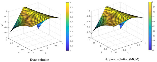
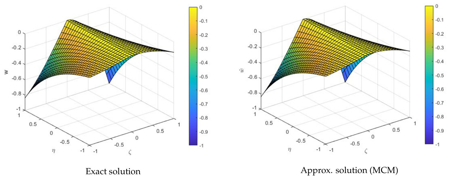
The above mentioned problem is a linear $2D$ parabolic problem with an interface. The MCM is used to solve the above mentioned problem numerically with constant coefficients $k_1(\zeta ,\eta ,\mathtt{t})=1$ and $k_2(\zeta ,\eta ,\mathtt{t})=1000$. A detailed comparison of MCM and HWCM is given in Table 1, which also highlights the errors of each model in terms of the MAE and RMSE. The MAE obtained through MCM for different numbers of grid points (GPs) demonstrates that the reliability of the proposed method increases as the number of GPs increases; this is a key advantage of MCM. For example, with $N=30$ GPs, an accuracy on the order of ${10}^{-5}$ is achieved. Furthermore, Figure 3 uses $3D$ plots for time step $\Delta t=0.05$ with $N=30$ to compare the numerical and exact solutions. These graphs further validate the reliability and accuracy of the suggested approach by demonstrating how closely the approximate and exact solutions match.

Table 1. Comparison of MCM and HWCM numerical results for Test Problem 1.

Proposed MCM						HWCM
$\mathit{N}$	$\mathit{dt}$	MAEs	RMSEs	${\mathcal{R}}_{\mathit{c}}\left(\mathit{N}\right)$	CPU Time (s)	$\mathit{N}$	$\mathit{dt}$	MAEs	CPU Time (s)
14	$0.05/14$	$5.1347\times {10}^{-4}$	$1.8764\times {10}^{-4}$	–	0.122037	$4\times 4$	$0.01/4$	$3.9250\times {10}^{-4}$	0.065036
20	$0.05/20$	$1.1237\times {10}^{-4}$	$3.5770\times {10}^{-5}$	2.192	0.434800	$8\times 8$	$0.01/8$	$1.3308\times {10}^{-4}$	1.139301
24	$0.05/24$	$4.5929\times {10}^{-5}$	$1.4329\times {10}^{-5}$	1.2908	0.495572	$16\times 16$	$0.01/16$	$3.1392\times {10}^{-5}$	31.430197
30	$0.05/30$	$2.9703\times {10}^{-5}$	$8.1590\times {10}^{-6}$	0.6288	1.368901	$32\times 32$	$0.01/32$	$5.7513\times {10}^{-6}$	1012.783061

Figure 3. Comparison between the exact and approximate solutions, $N=30$, $\Delta t=0.05$ and $c=7$ for Test Problem 1.

Test Problem 2.

The given initial-boundary value linear parabolic problem having single interface conditions is considered here:

$$w_{\mathtt{t}}-{\left(k(\zeta ,\eta ,\mathtt{t})w_{\zeta }\right)}_{\zeta }-{\left(k(\zeta ,\eta ,\mathtt{t})w_{\eta }\right)}_{\eta }=f(\zeta ,\eta ,\mathtt{t}),$$

where

$$k(\zeta ,\eta ,\mathtt{t})=\left\{\begin{array}{cc}{k}_1(\zeta ,\eta ,\mathtt{t}),\hfill & -1\le \zeta \le 0,-1\le \eta \le 1,\hfill \\ k_2(\zeta ,\eta ,\mathtt{t}),\hfill & 0\le \zeta \le 1,-1\le \eta \le 1.\hfill \end{array}\right.$$

The Dirichlet BCs are given by

$$\begin{array}{cccccc}\hfill w_1(-1,\eta ,\mathtt{t})& =e^{-\mathtt{t}}{e}^{-1}(sin\left(\eta \right)+{\eta }^2),\hfill & \hfill w_2(1,\eta ,\mathtt{t})& =e^{-\mathtt{t}}(-1-{\eta }^2),\hfill & \hfill & -1\le \eta \le 1,\hfill \\ \hfill w_1(\zeta ,-1,\mathtt{t})& =e^{-\mathtt{t}}{e}^{\zeta }({\zeta }^{2}sin(-1)+1),\hfill & \hfill w_1(\zeta ,1,\mathtt{t})& =e^{-\mathtt{t}}{e}^{\zeta }({\zeta }^{2}sin\left(1\right)+1),\hfill & \hfill & -1\le \zeta \le 0,\hfill \\ \hfill w_2(\zeta ,-1,\mathtt{t})& =e^{-\mathtt{t}}(-{\zeta }^2-1),\hfill & \hfill w_2(\zeta ,1,\mathtt{t})& =e^{-\mathtt{t}}({\zeta }^2-1),\hfill & \hfill & 0\le \zeta \le 1,\hfill \end{array}$$

and the interface conditions are

$$\begin{array}{ccc}\hfill & w_2(0,\eta ,\mathtt{t})-w_1(0,\eta ,\mathtt{t})=-2e^{-\mathtt{t}}{\eta }^2,\hfill & \hfill -1\le \eta \le 1,\\ \hfill & (\eta +1){\displaystyle \frac{\partial w_2}{\partial \zeta }}(0,\eta ,\mathtt{t})-({\eta }^2+1){\displaystyle \frac{\partial w_1}{\partial \zeta }}(0,\eta ,\mathtt{t})=e^{-\mathtt{t}}(-{\eta }^4-{\eta }^2),\hfill & \hfill -1\le \eta \le 1.\end{array}$$

In each subdomain, the function $f(\zeta ,\eta ,\mathtt{t})$ is calculated by utilizing the exact solution given below:

$$w(\zeta ,\eta ,\mathtt{t})=\left\{\begin{array}{cc}{w}_1(\zeta ,\eta ,\mathtt{t})=e^{-\mathtt{t}}{e}^{\zeta }({\zeta }^{2}sin\left(\eta \right)+{\eta }^2),\hfill & -1\le \zeta \le 0,-1\le \eta \le 1,\hfill \\ w_2(\zeta ,\eta ,\mathtt{t})=e^{-\mathtt{t}}(-{\zeta }^2-{\eta }^2),\hfill & 0\le \zeta \le 1,-1\le \eta \le 1.\hfill \end{array}\right.$$

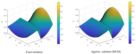
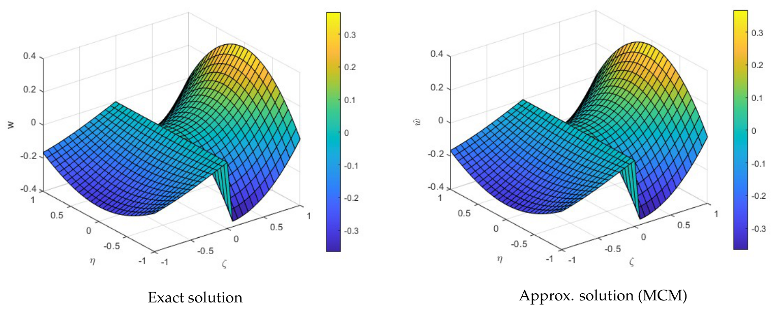
Another linear $2D$ PIP is considered, featuring variable coefficients $k_1(\zeta ,\eta ,\mathtt{t})=({\zeta }^2+{\eta }^2+1)$ and $k_2(\zeta ,\eta ,\mathtt{t})=(\zeta +\eta +1)$. The problem is numerically solved using the MCM. A comparative analysis with HWCM is presented in Table 2, reporting the MAE and RMSE for both methods. The results show that the accuracy of MCM improves with an increasing number of GPs, achieving an MAE of the order ${10}^{-5}$ for $N=30$. Additionally, Figure 4 provides $3D$ plots of the numerical and exact solutions at $\Delta t=0.05$ with $N=30$, clearly illustrating the reliability and high accuracy of the proposed method. Moreover, in the table, the computational rate of convergence $R_c\left(N\right)$ measures the reduction in error with increasing discretization level N. Positive values of $R_c\left(N\right)$ indicate convergence, while occasional negative values occur when the error at a finer resolution is slightly larger than that at the previous level. Such fluctuations are typically caused by round-off errors and numerical approximations when the errors become very small. Since the overall MAE and RMSE decrease as N increases, these isolated negative values do not affect the overall convergence of the proposed method.

Table 2. Comparison of MCM and HWCM numerical results for Test Problem 2.

Proposed MCM						HWCM
$\mathit{N}$	$\mathit{dt}$	MAEs	RMSEs	${\mathcal{R}}_{\mathit{c}}\left(\mathit{N}\right)$	CPU Time (s)	$\mathit{N}$	$\mathit{dt}$	MAEs	CPU Time (s)
14	$0.05/14$	$6.3237\times {10}^{-4}$	$1.8777\times {10}^{-4}$	–	0.357118	$4\times 4$	$0.01/4$	$1.5305\times {10}^{-3}$	0.084306
20	$0.05/20$	$1.6098\times {10}^{-4}$	$4.3853\times {10}^{-5}$	1.9739	0.308629	$8\times 8$	$0.01/8$	$6.8868\times {10}^{-4}$	1.403612
24	$0.05/24$	$2.2812\times {10}^{-4}$	$5.4122\times {10}^{-5}$	−0.50291	0.565159	$16\times 16$	$0.01/16$	$2.2270\times {10}^{-4}$	37.880220
30	$0.05/30$	$3.0187\times {10}^{-5}$	$7.8875\times {10}^{-5}$	2.9178	1.455750	$32\times 32$	$0.01/32$	$6.3413\times {10}^{-5}$	1205.107272

Figure 4. Comparison between the exact and approximate solutions, $N=30$, $\Delta t=0.05$ and $c=7$ for Test Problem 2.

Test Problem 3.

The given initial-boundary value linear parabolic problem having single interface conditions is considered here:

$$w_{\mathtt{t}}-{\left(k(\zeta ,\eta ,\mathtt{t})w_{\zeta }\right)}_{\zeta }-{\left(k(\zeta ,\eta ,\mathtt{t})w_{\eta }\right)}_{\eta }=f(\zeta ,\eta ,\mathtt{t}),$$

where

$$k(\zeta ,\eta ,\mathtt{t})=\left\{\begin{array}{cc}{k}_1(\zeta ,\eta ,\mathtt{t}),\hfill & -1\le \zeta \le 0,-1\le \eta \le 1,\hfill \\ k_2(\zeta ,\eta ,\mathtt{t}),\hfill & 0\le \zeta \le 1,-1\le \eta \le 1.\hfill \end{array}\right.$$

The Dirichlet BCs are given by

$$\begin{array}{cccccc}\hfill w_1(-1,\eta ,\mathtt{t})& =e^{-\mathtt{t}}sin(-1)cos\left(\eta \right),\hfill & \hfill w_2(1,\eta ,\mathtt{t})& =e^{-\mathtt{t}}(1-{\eta }^2),\hfill & \hfill & -1\le \eta \le 1,\hfill \\ \hfill w_1(\zeta ,-1,\mathtt{t})& =e^{-\mathtt{t}}sin\left(\zeta \right)cos(-1),\hfill & \hfill w_1(\zeta ,1,\mathtt{t})& =e^{-\mathtt{t}}sin\left(\zeta \right)cos\left(1\right),\hfill & \hfill & -1\le \zeta \le 0,\hfill \\ \hfill w_2(\zeta ,-1,\mathtt{t})& =e^{-\mathtt{t}}({\zeta }^2-1),\hfill & \hfill w_2(\zeta ,1,\mathtt{t})& =e^{-\mathtt{t}}({\zeta }^2-1),\hfill & \hfill & 0\le \zeta \le 1,\hfill \end{array}$$

and the interface conditions are

$$\begin{array}{ccc}\hfill & w_2(0,\eta ,\mathtt{t})-w_1(0,\eta ,\mathtt{t})=-e^{-\mathtt{t}}{\eta }^2,\hfill & \hfill -1\le \eta \le 1,\\ \hfill & k_2(0,\eta ,\mathtt{t}){\displaystyle \frac{\partial w_2}{\partial \zeta }}(0,\eta ,\mathtt{t})-k_1(0,\eta ,\mathtt{t}){\displaystyle \frac{\partial w_1}{\partial \zeta }}(0,\eta ,\mathtt{t})=-e^{-\mathtt{t}}cos\left(\eta \right),\hfill & \hfill -1\le \eta \le 1.\end{array}$$

In each subdomain, the function $f(\zeta ,\eta ,\mathtt{t})$ is calculated by utilizing the exact solution given below:

$$w(\zeta ,\eta ,\mathtt{t})=\left\{\begin{array}{cc}{w}_1(\zeta ,\eta ,\mathtt{t})=e^{-\mathtt{t}}sin\left(\zeta \right)cos\left(\eta \right),\hfill & -1\le \zeta \le 0,-1\le \eta \le 1,\hfill \\ w_2(\zeta ,\eta ,\mathtt{t})=e^{-\mathtt{t}}({\zeta }^2-{\eta }^2),\hfill & 0\le \zeta \le 1,-1\le \eta \le 1.\hfill \end{array}\right.$$

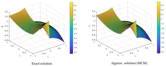
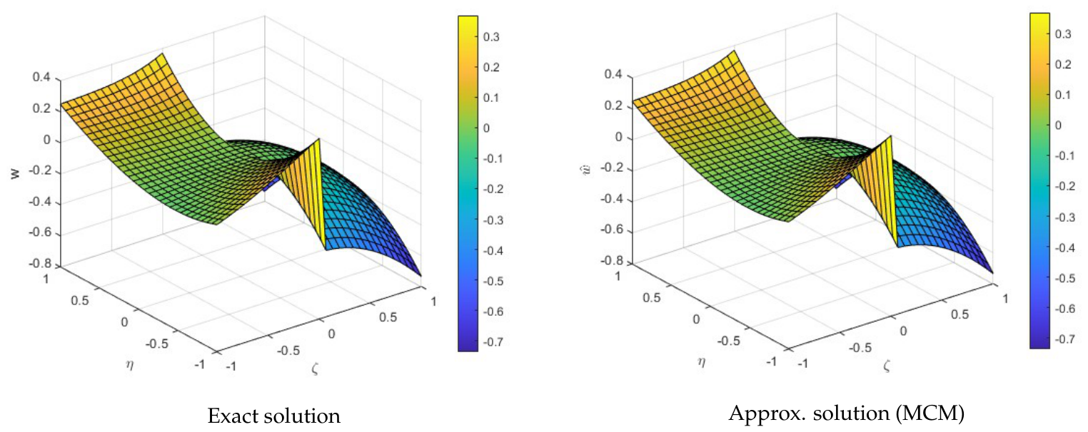
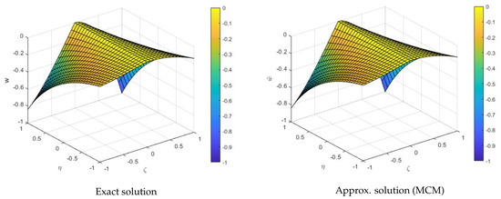
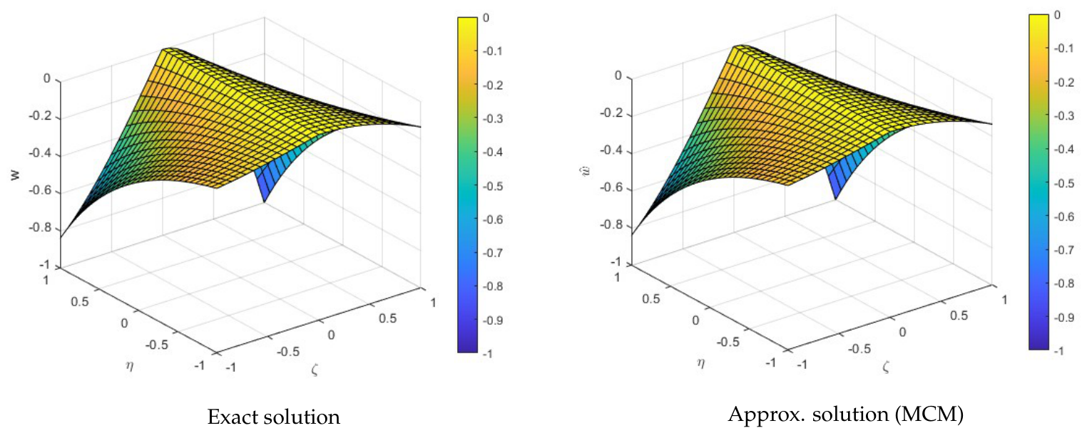
This linear $2D$ parabolic interface problem with constant coefficients $k_1(\zeta ,\eta ,\mathtt{t})=1$ and $k_2(\zeta ,\eta ,\mathtt{t})=10$ is numerically solved using the MCM. Table 3 presents a detailed comparison with HWCM, highlighting the MAE and RMSE values. The results show that the accuracy of MCM improves with more GPs, achieving errors as low as ${10}^{-5}$ for $N=28$. Figure 5 further supports this through $3D$ graphs comparing the numerical and exact solutions at $\Delta t=0.05$, demonstrating the reliability and precision of the method.

Table 3. Comparison of MCM and HWCM numerical results for Test Problem 3.

Proposed MCM					HWCM
$\mathit{N}$	$\mathit{dt}$	MAEs	RMSEs	${\mathcal{R}}_{\mathit{c}}\left(\mathit{N}\right)$	$\mathit{N}$	$\mathit{dt}$	MAEs
10	0.05/10	$2.7183\times {10}^{-4}$	$1.1854\times {10}^{-4}$	-	$4\times 4$	0.01/4	$2.5751\times {10}^{-4}$
14	0.05/14	$4.9584\times {10}^{-5}$	$1.9729\times {10}^{-5}$	2.4548	$8\times 8$	0.01/8	$8.1714\times {10}^{-4}$
20	0.05/20	$1.8878\times {10}^{-5}$	$6.4914\times {10}^{-6}$	1.3932	$16\times 16$	0.01/16	$2.3105\times {10}^{-5}$
28	0.05/28	$2.1361\times {10}^{-5}$	$7.2674\times {10}^{-6}$	−0.17827	$32\times 32$	0.01/32	$6.3008\times {10}^{-6}$

Figure 5. Comparison between the exact and approximate solutions, $N=28$, $\Delta t=0.05$ and $c=7$ for Test Problem 3.

Test Problem 4.

The given initial-boundary value nonlinear parabolic problem having interface conditions is considered here:

$$w_{\mathtt{t}}-{\left(k(\zeta ,\eta ,\mathtt{t})w_{\zeta }\right)}_{\zeta }-{\left(k(\zeta ,\eta ,\mathtt{t})w_{\eta }\right)}_{\eta }-2w^2(\zeta ,\eta ,\mathtt{t})=f(\zeta ,\eta ,\mathtt{t})$$

where

$$k(\zeta ,\eta ,\mathtt{t})=\left\{\begin{array}{cc}{k}_1(\zeta ,\eta ,\mathtt{t}),\hfill & -1\le \zeta \le 0,-1\le \eta \le 1,\hfill \\ k_2(\zeta ,\eta ,\mathtt{t}),\hfill & 0\le \zeta \le 1,-1\le \eta \le 1.\hfill \end{array}\right.$$

The Dirichlet BCs are given by

$$\begin{array}{cccccc}\hfill w_1(-1,\eta ,\mathtt{t})& =e^{-\mathtt{t}}{e}^{\eta }sin(-1),\hfill & \hfill w_2(1,\eta ,\mathtt{t})& =-e^{-\mathtt{t}}{e}^{\eta },\hfill & \hfill & -1\le \eta \le 1,\hfill \\ \hfill w_1(\zeta ,-1,\mathtt{t})& =e^{-\mathtt{t}}{e}^{-1}sin\left(\zeta \right),\hfill & \hfill w_1(\zeta ,1,\mathtt{t})& =e^{-\mathtt{t}}esin\left(\zeta \right),\hfill & \hfill & -1\le \zeta \le 0,\hfill \\ \hfill w_2(\zeta ,-1,\mathtt{t})& =-e^{-\mathtt{t}}{e}^{-1}{\zeta }^2,\hfill & \hfill w_2(\zeta ,1,\mathtt{t})& =-e^{-\mathtt{t}}e{\zeta }^2,\hfill & \hfill & 0\le \zeta \le 1,\hfill \end{array}$$

and the interface conditions are

$$\begin{array}{ccc}\hfill & w_2(0,\eta ,\mathtt{t})-w_1(0,\eta ,\mathtt{t})=0,\hfill & \hfill -1\le \eta \le 1,\\ \hfill & k_2(0,\eta ,\mathtt{t}){\displaystyle \frac{\partial w_2}{\partial \zeta }}(0,\eta ,\mathtt{t})-k_1(0,\eta ,\mathtt{t}){\displaystyle \frac{\partial w_1}{\partial \zeta }}(0,\eta ,\mathtt{t})=-e^{-\mathtt{t}}{e}^{\eta },\hfill & \hfill -1\le \eta \le 1.\end{array}$$

In each subdomain, the function $f(\zeta ,\eta ,\mathtt{t})$ is calculated by utilizing the exact solution given below:

$$w(\zeta ,\eta ,\mathtt{t})=\left\{\begin{array}{cc}{w}_1(\zeta ,\eta ,\mathtt{t})=e^{-\mathtt{t}}{e}^{\eta }sin\left(\zeta \right),\hfill & -1\le \zeta \le 0,-1\le \eta \le 1,\hfill \\ w_2(\zeta ,\eta ,\mathtt{t})=-e^{-\mathtt{t}}{e}^{\eta }{\zeta }^2,\hfill & 0\le \zeta \le 1,-1\le \eta \le 1.\hfill \end{array}\right.$$

The test problem mentioned above is a nonlinear $2D$ parabolic problem with an interface. The MCM is used to solve the above mentioned example numerically with constant coefficient $k_1(\zeta ,\eta ,\mathtt{t})=1$ and $k_2(\zeta ,\eta ,\mathtt{t})=1000$. A detailed comparison of MCM and HWCM is given in Table 4, which also highlights the errors of each model in terms of the MAE and RMSE. In Test Problem 4, QNLT is used to solve the nonlinear system. The MAE obtained through MCM for different numbers of GPs demonstrates that the reliability of the proposed method increases as the number of GPs increases; this is a key advantage of MCM. For example, with $N=30$ GPs, an accuracy on the order of ${10}^{-5}$ is achieved. Furthermore, Figure 6 uses $3D$ plots for the time step, $\Delta t=0.05$ with $N=30$ to compare the exact and numerical solutions. These graphs further validate the reliability and accuracy of the suggested approach by demonstrating how closely the approximate and exact solutions match.

Table 4. Comparison of MCM and HWCM numerical results for Test Problem 4.

Proposed MCM					HWCM
$\mathit{N}$	$\mathit{dt}$	MAEs	RMSEs	${\mathcal{R}}_{\mathit{c}}\left(\mathit{N}\right)$	$\mathit{N}$	$\mathit{dt}$	MAEs
14	0.05/14	$8.6242\times {10}^{-4}$	$3.3187\times {10}^{-4}$	-	$4\times 4$	0.01/4	$3.7213\times {10}^{-4}$
20	0.05/20	$1.7803\times {10}^{-4}$	$5.8785\times {10}^{-5}$	2.2763	$8\times 8$	0.01/8	$1.2188\times {10}^{-4}$
24	0.05/24	$6.9605\times {10}^{-5}$	$2.0926\times {10}^{-5}$	1.3549	$16\times 16$	0.01/16	$2.8662\times {10}^{-5}$
30	0.05/30	$2.7350\times {10}^{-5}$	$8.3249\times {10}^{-6}$	1.3477	$32\times 32$	0.01/32	$5.2505\times {10}^{-6}$

Figure 6. Comparison between the exact and approximate solutions, $N=30$, $\Delta t=0.05$ and $c=7$ for Test Problem 4.

Test Problem 5.

The given initial-boundary value nonlinear parabolic problem having interface conditions is considered here:

$$w_{\mathtt{t}}-{\left(k(\zeta ,\eta ,\mathtt{t})w_{\zeta }\right)}_{\zeta }-{\left(k(\zeta ,\eta ,\mathtt{t})w_{\eta }\right)}_{\eta }-w{w}_{\zeta }(\zeta ,\eta ,\mathtt{t})=f(\zeta ,\eta ,\mathtt{t}),$$

where

$$k(\zeta ,\eta ,\mathtt{t})=\left\{\begin{array}{cc}{k}_1(\zeta ,\eta ,\mathtt{t}),\hfill & -1\le \zeta \le 0,-1\le \eta \le 1,\hfill \\ k_2(\zeta ,\eta ,\mathtt{t}),\hfill & 0\le \zeta \le 1,-1\le \eta \le 1.\hfill \end{array}\right.$$

The Dirichlet BCs are given by

$$\begin{array}{cccccc}\hfill w_1(-1,\eta ,\mathtt{t})& =e^{-\mathtt{t}}{e}^{\eta }sin(-1),\hfill & \hfill w_2(1,\eta ,\mathtt{t})& =-e^{-\mathtt{t}}{e}^{\eta },\hfill & \hfill & -1\le \eta \le 1,\hfill \\ \hfill w_1(\zeta ,-1,\mathtt{t})& =e^{-\mathtt{t}}{e}^{-1}sin\left(\zeta \right),\hfill & \hfill w_1(\zeta ,1,\mathtt{t})& =e^{-\mathtt{t}}esin\left(\zeta \right),\hfill & \hfill & -1\le \zeta \le 0,\hfill \\ \hfill w_2(\zeta ,-1,\mathtt{t})& =-e^{-\mathtt{t}}{e}^{-1}{\zeta }^2,\hfill & \hfill w_2(\zeta ,1,\mathtt{t})& =-e^{-\mathtt{t}}e{\zeta }^2,\hfill & \hfill & 0\le \zeta \le 1,\hfill \end{array}$$

and the interface conditions are

$$\begin{array}{ccc}\hfill & w_2(0,\eta ,\mathtt{t})-w_1(0,\eta ,\mathtt{t})=0,\hfill & \hfill -1\le \eta \le 1,\\ \hfill & k_2(0,\eta ,\mathtt{t}){\displaystyle \frac{\partial w_2}{\partial \zeta }}(0,\eta ,\mathtt{t})-k_1(0,\eta ,\mathtt{t}){\displaystyle \frac{\partial w_1}{\partial \zeta }}(0,\eta ,\mathtt{t})=-e^{-\mathtt{t}}{e}^{\eta },\hfill & \hfill -1\le \eta \le 1.\end{array}$$

In each subdomain, the function $f(\zeta ,\eta ,\mathtt{t})$ is calculated by utilizing the exact solution given below:

$$w(\zeta ,\eta ,\mathtt{t})=\left\{\begin{array}{cc}{w}_1(\zeta ,\eta ,\mathtt{t})=e^{-\mathtt{t}}{e}^{\eta }sin\left(\zeta \right),\hfill & -1\le \zeta \le 0,-1\le \eta \le 1,\hfill \\ w_2(\zeta ,\eta ,\mathtt{t})=-e^{-\mathtt{t}}{e}^{\eta }{\zeta }^2,\hfill & 0\le \zeta \le 1,-1\le \eta \le 1.\hfill \end{array}\right.$$

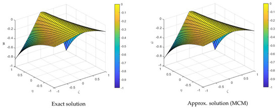
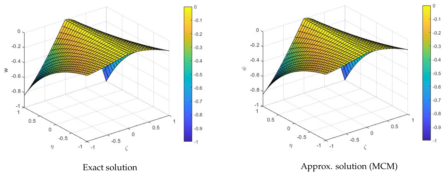
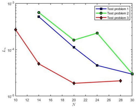
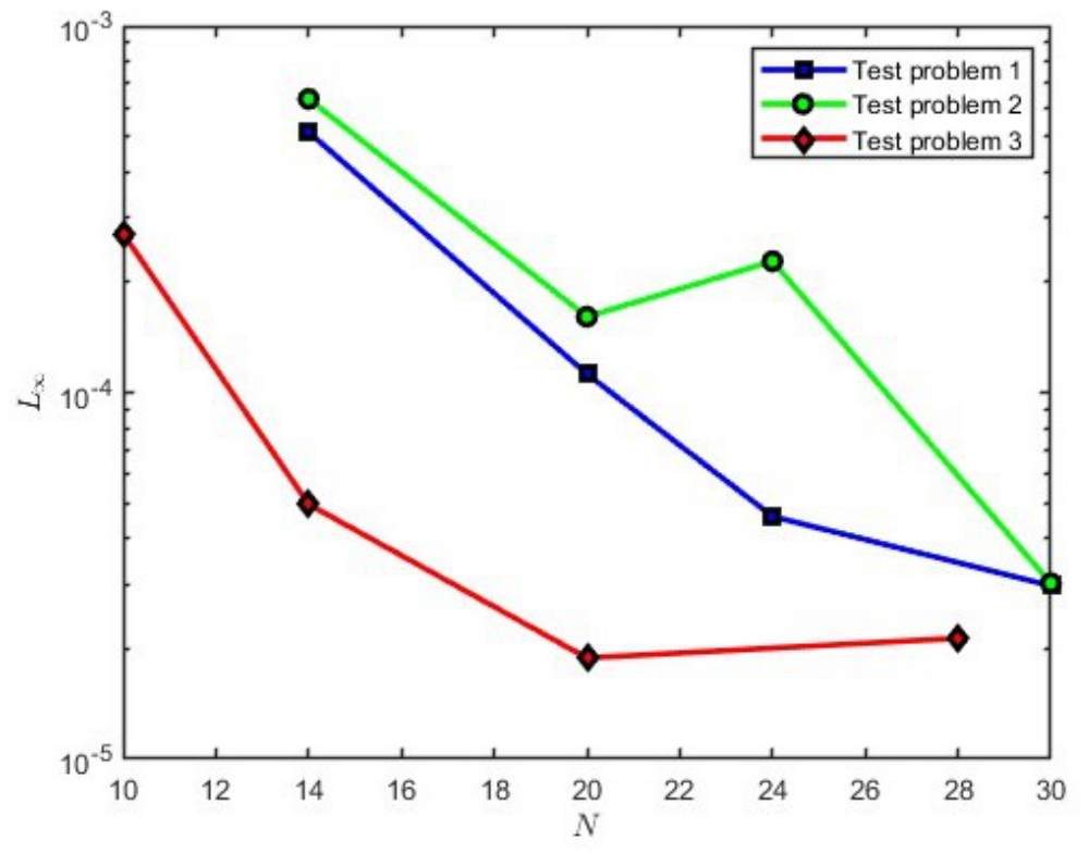
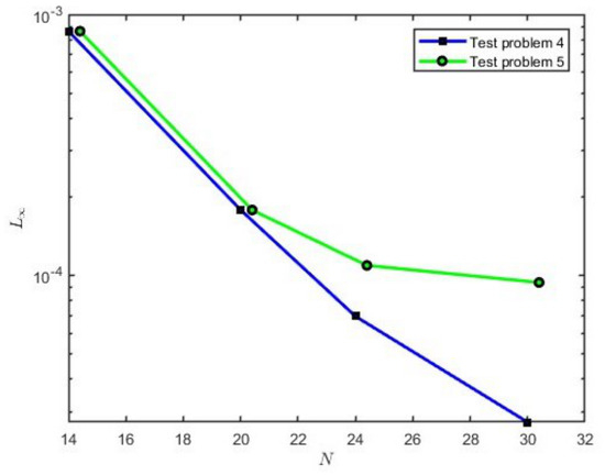
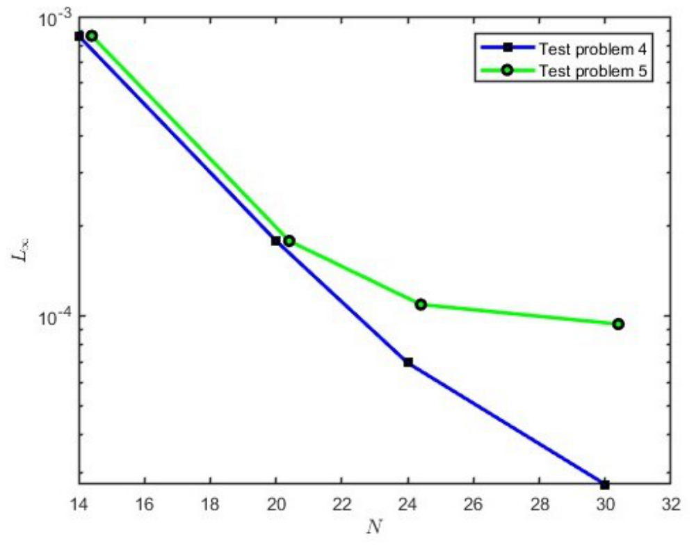
The above test problem is also a nonlinear $2D$ PIP with constant coefficients $k_1(\zeta ,\eta ,\mathtt{t})=1$ and $k_2(\zeta ,\eta ,\mathtt{t})=1000$. The MCM is employed to numerically solve this example, using the QNLT for handling nonlinearity. A comparative evaluation of MCM and HWCM is provided in Table 5, presenting the MAE and RMSE for both methods. The results confirm that the accuracy of MCM improves with an increasing number of GPs, reaching an MAE of the order of ${10}^{-5}$ for $N=30$. Additionally, Figure 7 presents $3D$ plots of the numerical and exact solutions at a time step $\Delta t=0.05$ with $N=30$, further assessing the precision and robustness of the proposed method through close agreement between the two solutions. Moreover, the graphical representations of the MAE for the different problems are presented in Figure 8 and Figure 9.

Table 5. Comparison of MCM numerical results for Test Problem 5.

Proposed MCM
$\mathit{N}$	$\mathit{dt}$	MAEs	RMSEs	CPU Time (s)	${\mathcal{R}}_{\mathit{c}}\left(\mathit{N}\right)$
14	0.05/14	$8.6232\times {10}^{-4}$	$3.2373\times {10}^{-4}$	3.609025	-
20	0.05/20	$1.7794\times {10}^{-4}$	$6.1119\times {10}^{-5}$	23.687894	2.2768
24	0.05/24	$1.0907\times {10}^{-4}$	$3.4896\times {10}^{-5}$	71.180985	0.70614
30	0.05/30	$9.3821\times {10}^{-5}$	$2.7945\times {10}^{-5}$	298.796883	0.21727

Figure 7. Comparison between the exact and approximate solutions, $N=30$, $\Delta t=0.05$ and $c=7$ for Test Problem 5.

Figure 8. Maximum absolute errors of the proposed method for linear test problems at $N=30$, $\Delta t=0.05$ and $c=7$.

Figure 9. Maximum absolute errors of the proposed method for nonlinear test problems at $N=30$, $\Delta t=0.05$ and $c=7$.

6. Conclusions

In this paper, a new method for solving PIPs is introduced. The proposed method integrates the FDM with the MCM using MQ RBFs. To assess its performance, several linear and nonlinear examples are examined, both with constant and variable coefficients. The findings demonstrate that the proposed method delivers high accuracy and computational efficiency in both types of models. Furthermore, the results show that increasing the number of GPs consistently improves the accuracy, indicating the flexibility and adaptability of the method. However, its computational cost may increase significantly as the number of nodes grows. In addition, accurately enforcing interface conditions for problems with highly complex geometries or strong discontinuities may require special treatments, which can affect the efficiency and implementation simplicity. The MQ-RBF shape parameter significantly influences both the accuracy and conditioning of the resulting algebraic system. In this work, the shape parameter was selected empirically through a trial-and-error procedure. Several values were examined, and the reported value was found to provide the best overall performance in terms of accuracy and stability for the test problems considered. Compared to HWCM, the proposed method yields improved results, especially in terms of the MAE and RMSE, while requiring fewer nodes. This highlights the method’s capacity to achieve high precision with a lower computational cost. Furthermore, the stability analysis of the proposed method focuses on the spatial discretization, while the temporal discretization is treated explicitly. The use of Forward Euler does not compromise the validity of the results, provided that the time step restriction is respected. More robust implicit schemes, such as Backward Euler, are unconditionally stable and may be employed as a straightforward extension of the present framework for stiff or large-scale problems. Future work will focus on extending this approach to $2D$ and three-dimensional PIPs involving multiple interfaces. Moreover, exploring its application to fractional interface problems and irregular interface geometries remains an open and promising area for further research.

References

- Liu, W.K.; Liu, Y.; Farrell, D.; Zhang, L.; Wang, S.; Fukui, Y.; Patankar, N.; Zhang, Y.; Bajaj, C.; Hong, J.L. Immersed finite element method and its applications to biological systems. Comput. Methods Appl. Mech. Eng. 2006, 195, 1722–1749. [Google Scholar] [CrossRef] [Scilit] [PubMed]
- Adel, M.; Khader, M.M.; Babatin, M.M.; Youssef, M.Z. Numerical investigation for the fractional model of pollution for a system of lakes using the SCM based on the Appell type Changhee polynomials. AIMS Math. 2023, 8, 31104–31117. [Google Scholar] [CrossRef] [Scilit]
- Tadmor, E. A review of numerical methods for non-linear partial differential equations. Bull. Am. Math. Soc. 2012, 49, 507–554. [Google Scholar] [CrossRef] [Scilit]
- Aziz, I.; Islam, S.; Haider, N. Meshless and multi-resolution collocation techniques for parabolic interface models. J. Comput. Appl. Math. 2018, 335, 313–332. [Google Scholar] [CrossRef] [Scilit]
- Wei, Z.; Li, C.; Zhao, S. A spatially second order alternating direction implicit (ADI) method for three dimensional parabolic interface problems. Comput. Math. Appl. 2018, 75, 2173–2192. [Google Scholar] [CrossRef] [Scilit]
- Shi, D.; Wang, J. Unconditional super convergence analysis of conforming finite element for nonlinear parabolic equations. Appl. Math. Comput. 2017, 294, 216–226. [Google Scholar] [CrossRef] [Scilit]
- Benes, M.; Kruis, J. Multi-time-step domain decomposition and coupling methods for nonlinear parabolic problems. Appl. Math. Comput. 2018, 319, 444–460. [Google Scholar] [CrossRef] [Scilit]
- Mohanty, R.K.; Setia, N. A new high accuracy two-level implicit off-step discretization for the system of three space dimensional quasi-linear parabolic partial differential equations. Comput. Math. Appl. 2015, 69, 1096–1113. [Google Scholar] [CrossRef] [Scilit]
- Tan, W.C.; Hoang, V.H. High dimensional finite element method for multiscale nonlinear monotone parabolic equations. J. Comput. Appl. Math. 2019, 345, 471–500. [Google Scholar] [CrossRef] [Scilit]
- Abdulla, U.G.; Du, J.; Prinkey, A.; Ondracek, C.; Parimoo, S. Evolution of interfaces for the nonlinear double degenerate parabolic equation of turbulent filtration with absorption. Math. Comput. Simul. 2018, 153, 59–82. [Google Scholar] [CrossRef] [Scilit]
- Faheem, M.; Asif, M.; Haider, N.; Amin, R.; Al-Mdallal, Q.M. Hybrid Haar wavelet and meshfree methods for hyperbolic double interface problems: Numerical implementations and comparative performance analysis. Partial. Differ. Equ. Appl. Math. 2024, 11, 1–15. [Google Scholar] [CrossRef] [Scilit]
- Asif, M.; Farooq, U.; Riaz, M.B.; Bilal, F.; Haider, N. Numerical assessment of hyperbolic type double interface problems via Haar wavelets. Partial. Differ. Equ. Appl. Math. 2024, 10, 1–10. [Google Scholar] [CrossRef] [Scilit]
- Asif, M.; Bilal, F.; Shakeel, M.; Bilal, R.; Haider, N.; Abdelmohsenc, S.A.; Eldind, S.M. An efficient algorithm for the numerical solution of telegraph interface model with discontinuous coefficients via Haar wavelets. Alex. Eng. J. 2023, 72, 275–285. [Google Scholar] [CrossRef] [Scilit]
- Rana, G.; Asif, M.; Haider, N.; Bilal, R.; Ahsan, M.; Al-Mdallal, Q.; Jarad, F. A modified algorithm based on Haar wavelets for the numerical simulation of interface models. J. Funct. Spaces 2022, 2022, 1541486. [Google Scholar] [CrossRef] [Scilit]
- Asif, M.; Bilal, F.; Haider, N.; Jarad, F. Robust numerical techniques for modeling telegraph equations in multi-scale and heterogeneous environments. J. Appl. Math. Comput. 2025, 71, 6585–6620. [Google Scholar] [CrossRef] [Scilit]
- Asif, M.; Gul, T.; Riaz, M.B.; Bilal, F. Solution of nonlinear telegraph equation with discontinuities along the transmission line using meshless collocation method. Partial. Differ. Equ. Appl. Math. 2025, 2025, 101219. [Google Scholar] [CrossRef] [Scilit]
- Asif, M.; Akhtar, N.; Khan, F.; Bilal, F.; Popa, I.L. Numerical Treatment of Hyperbolic-Type Problems with Single and Double Interfaces via Meshless Method. Axioms 2025, 14, 621. [Google Scholar] [CrossRef] [Scilit]
- Shams Ul Haq, K.; Asif, M.; Faheem, M.; Popa, I.L. Capturing Discontinuities with Precision: A Numerical Exploration of 3D Telegraph Interface Models via Multi-Resolution Technique. Mathematics 2025, 13, 2391. [Google Scholar] [CrossRef] [Scilit]
- Nicomedes, W.L.; Mesquita, R.C.; Moreira, F.J.S. A meshless local Petrov–Galerkin method for three-dimensional scalar problems. IEEE Trans. Magn. 2011, 47, 1214–1217. [Google Scholar] [CrossRef] [Scilit]
- Nicomedes, W.L.; Mesquita, R.C.; Moreira, F.J.S. The meshless local Petrov–Galerkin method in two-dimensional electromagnetic wave analysis. IEEE Trans. Antennas Propag. 2012, 60, 1957–1968. [Google Scholar] [CrossRef] [Scilit]
- Lin, J.; Chen, C.; Wang, F.; Dangal, T. Method of particular solutions using polynomial basis functions for the simulation of plate bending vibration problems. Appl. Math. Model. 2017, 49, 452–469. [Google Scholar] [CrossRef] [Scilit]
- Lin, J.; Chen, W.; Wang, F. A new investigation into regularization techniques for the method of fundamental solutions. Math. Comput. Simul. 2011, 81, 1144–1152. [Google Scholar] [CrossRef] [Scilit]
- Karageorgis, A.; Fairweather, G. The method of fundamental solutions for axisymmetric potential problems. Int. J. Numer. Methods Eng. 1999, 44, 1653–1669. [Google Scholar] [CrossRef]
- Alves, C.J.; Antunes, P.R. The method of fundamental solutions applied to the calculation of eigensolutions for 2D plates. Int. J. Numer. Methods Eng. 2009, 77, 177–194. [Google Scholar] [CrossRef] [Scilit]
- Lin, J.; Chen, W.; Chen, C. Numerical treatment of acoustic problems with boundary singularities by the singular boundary method. J. Sound Vib. 2014, 333, 3177–3188. [Google Scholar] [CrossRef] [Scilit]
- Lin, J.; Zhang, C.; Sun, L.; Lu, J. Simulation of seismic wave scattering by embedded cavities in an elastic half-plane using the novel singular boundary method. Adv. Appl. Math. Mech. 2018, 10, 322–342. [Google Scholar] [CrossRef] [Scilit]
- Chen, W. Symmetric boundary knot method. Eng. Anal. Bound. Elem. 2002, 26, 489–494. [Google Scholar] [CrossRef] [Scilit]
- Jin, B.; Zheng, Y. Boundary knot method for some inverse problems associated with the Helmholtz equation. Int. J. Numer. Methods Eng. 2005, 62, 1636–1652. [Google Scholar] [CrossRef] [Scilit]
- Lin, J.; Chen, W.; Sze, K. A new radial basis function for Helmholtz problems. Eng. Anal. Bound. Elem. 2012, 36, 1923–1930. [Google Scholar] [CrossRef] [Scilit]
- ul Islam, S.; Ahmad, M. Meshless analysis of elliptic interface boundary value problems. Eng. Anal. Bound. Elem. 2018, 92, 38–49. [Google Scholar] [CrossRef] [Scilit]
- Zerroukat, M.; Power, H.; Chen, C.S. A numerical method for heat transfer problems using collocation and radial basis functions. Int. J. Numer. Methods Eng. 1998, 42, 1263–1278. [Google Scholar] [CrossRef] [Scilit]
- Ahmad, I.; ul Islam, S.; Khaliq, A.Q.M. Local RBF method for multi-dimensional partial differential equations. Comput. Math. Appl. 2017, 74, 292–324. [Google Scholar] [CrossRef] [Scilit]
- ul Islam, S.; Ahmad, I. Local meshless method for PDEs arising from models of wound healing. Appl. Math. Model. 2017, 48, 688–710. [Google Scholar] [CrossRef] [Scilit]
- Shin, B.C.; Jung, J.H. Spectral collocation and radial basis function methods for one-dimensional interface problems. Appl. Numer. Math. 2011, 61, 911–928. [Google Scholar] [CrossRef] [Scilit]
- Jamil, M.; Ng, E. Evaluation of meshless radial basis collocation method (RBCM) for heterogeneous conduction and simulation of temperature inside the biological tissues. Int. J. Therm. Sci. 2013, 68, 42–52. [Google Scholar] [CrossRef] [Scilit]
- Martin, B.; Fornberg, B. Seismic modeling with radial basis function–generated finite differences (RBF–FD)—A simplified treatment of interfaces. J. Comput. Phys. 2017, 35, 828–845. [Google Scholar] [CrossRef] [Scilit]
- Martin, B.; Fornberg, B. Using radial basis function–generated finite differences (RBF–FD) to solve heat transfer equilibrium problems in domains with interfaces. Eng. Anal. Bound. Elem. 2017, 79, 38–48. [Google Scholar] [CrossRef] [Scilit]
- Verma, R.; Kalita, J.C. Numerical Simulation of Phase Change Dual-Phase-Lag Bioheat Model with Nanocryosurgery Using Radial Basis Function Meshfree Approach. ASME J. Heat Mass Transf. 2025, 147, 061201. [Google Scholar] [CrossRef] [Scilit]
- Sakariya, H.; Verma, R.; Kumar, S. Numerical Simulation of the Time-Fractional DPL Bioheat Model with Phase Change Using Meshfree RBFs Approach. Comput. Math. Appl. 2026, 211, 76–93. [Google Scholar] [CrossRef] [Scilit]
- Kumar Meena, R.; Kumar, S. Semi-Analytical Solutions of the Multi-Dimensional Time-Fractional Solitary Water Wave Equations Using RPS Method. Math. Methods Appl. Sci. 2025, 48, 6208–6221. [Google Scholar] [CrossRef] [Scilit]
- Buhmann, M.D. Radial basis functions. Acta Numer. 2000, 9, 1–38. [Google Scholar] [CrossRef] [Scilit]
- Hardy, R.L. Multiquadric equations of topography and other irregular surfaces. J. Geophys. Res. 1971, 76, 1905–1915. [Google Scholar] [CrossRef] [Scilit]
- Rippa, S. An algorithm for selecting a good value for the parameter c in radial basis function interpolation. Adv. Comput. Math. 1999, 11, 193–210. [Google Scholar] [CrossRef] [Scilit]
- Huang, C.; Lee, C.; Cheng, A. Error estimate, optimal shape factor, and high precision computation of multiquadric collocation method. Eng. Anal. Bound. Elem. 2007, 31, 614–623. [Google Scholar] [CrossRef] [Scilit]
- Sun, H.; Mei, L.; Lin, Y. A new algorithm based on improved Legendre orthonormal basis for solving second-order BVPs. Appl. Math. Lett. 2021, 112, 106732. [Google Scholar] [CrossRef] [Scilit]
- LeVeque, R.J. Finite Difference Methods for Ordinary and Partial Differential Equations; Society for Industrial and Applied Mathematics (SIAM): Philadelphia, PA, USA, 2007; pp. xvi+341. [Google Scholar]
Disclaimer/Publisher’s Note: The statements, opinions and data contained in all publications are solely those of the individual author(s) and contributor(s) and not of MDPI and/or the editor(s). MDPI and/or the editor(s) disclaim responsibility for any injury to people or property resulting from any ideas, methods, instructions or products referred to in the content. |
© 2026 by the authors. Licensee MDPI, Basel, Switzerland. This article is an open access article distributed under the terms and conditions of the Creative Commons Attribution (CC BY) license.