Parameter Estimation for Modeling and Simulation of Multimodal Membrane Chromatography

Abstract

Protein chromatography, the process of separating desired proteins from other elements in a chemical solution, is used widely in the manufacturing of biotherapeutics. Many parameters involved in this process must be tested extensively during process development, which results in higher costs of the biotherapeutics. Modeling and simulation of the chromatography process could reduce the amount of time and resources spent on running live experiments, potentially lowering therapeutic costs. In this work, we consider the transport equation coupled with adsorption isotherm equations to model the process using a porous membrane as the medium for protein adsorption. For the adsorption isotherm models, we consider both an explicit function and an implicitly defined relationship. We use a semi-implicit, finite element solution implemented in FEniCS to solve the modeling equations and simulate the adsorption phase of membrane chromatography. We conduct an initial parameter space investigation to establish acceptable ranges on each parameter and then apply numerical optimization methods to determine optimal parameter values for the modeling equations. We solve the single-parameter optimization problem by applying a line search algorithm and a multi-parameter optimization problem using built-in functionality in FEniCS which applies the adjoint method. The single-parameter optimization algorithm is applied with an explicit adsorption model while the multi-parameter optimization algorithm is applied to both the explicitly and implicitly defined adsorption models. Both algorithms yield optimal parameter values that provide much more accurate simulation results. Last, we conduct a sensitivity analysis to establish which parameters most affect the model solution in an effort to reduce computational effort in the multi-parameter optimization problem. Results indicate that two parameters most affect the optimization results and suggest that the multi-objective optimization could be modified to adjust certain parameter values at different simulation times to reduce the computation time.

1. Introduction

The chromatography process separates a desired element, for example a particular protein, from a solution [1,2]. There are three main steps in the chromatography process. Initially, in the adsorption step, a fluid containing a high concentration of the desired protein passes through the chromatography column allowing the protein to adsorb to the materials in the column. When a significant amount of protein appears in the effluent, the fluid exiting the column, no more concentration is fed into the column, which ends the adsorption phase of the chromatography process. Next, a wash buffer is pushed through the column to remove any weakly adsorbed proteins and unwanted substances that may have bonded with the membrane. Last in the elution stage, a solution is pushed through the column to remove the desired protein from the column [3].

Historically, resin-bead chromatography has been used to separate the target protein. While resin-bead chromatography is reliable, this strategy is diffusion-based, and relies on the protein adhering to the surface of a resin bead and subsequently diffusing into the bead core. This process is time-consuming, delaying the production of these therapies and hence limiting their availability to the population.

This process is widely used in drug manufacturing within the pharmaceutical industry [1,4]. The chromatographic process yields precise separation of high quality materials, but the lengthy process and economic weight often lead to using alternate methods which are less accurate but more convenient [1]. To obtain better protein separation in less time, running several live experiments to obtain the correct experimental setup can be very costly, while using an accurate model to simulate the best possible outcome is significantly more economic [2]. Consequently, optimization of the chromatography process through the use of mathematical modeling could lead to more efficient and higher quality drug manufacturing.

Both statistical models and mechanistic models can be applied to model the chromatography process. Bernau et al. discussed the benefits and limitations of modeling this process using data-driven, mechanistic, and hybrid models [2]. Obtaining the correct parameter values for a model is imperative to ensure accurate results when optimizing the chromatography model [2,5]. Although initial approximations for some parameter values can be obtained through several live experiments as outlined in the studies of Tarafder et al. and Bernau et al. [1,2], there is still some variability in these parameter values, and other model parameters, such as dispersion coefficients, must simply be estimated based on ranges available in the literature.

While mechanistic models are very beneficial for use with optimization, they can be especially sensitive to excessive noise in data [2]. Lalli et al. obtained accurate results between models of the chromatography process and experimentally obtained data. They discuss the importance of the use of dispersion coefficients in obtaining accurate results as opposed to only considering membrane pore size distribution. From pulse testing data, they discuss the use of moment analysis on the effluent peaks to determine both the void fraction and the axial dispersion coefficient; they calculate and test multiple dispersion coefficients in their model determining that the dispersion coefficient is an important parameter for membrane chromatography modeling [6]. Hence, having accurate parameter values, particularly dispersion coefficient values, is essential to accurately modeling and optimizing the chromatography process.

Tarafder et al. used initial parameter values along with a Non-dominated Sorting Genetic Algorithm (NSGA) to optimize productivity, solvent consumption, and yield with a constraint on the level of purity [1]. They modeled resin-bead chromatography, a reliable diffusion-based form of chromatography, and their model incorporated non-instantaneous adsorption in which a lumped kinetic equilibrium equation was coupled with the other modeling equations [1]. They concluded that a yield of 90% can be obtained for their model without sacrificing productivity, and reducing the purity constraint resulted in improved productivity for all yield percentages [1]. Heinonen sought to optimize similar objectives in a multi-column chromatographic process using a general differential evolution algorithm (GDE) to adjust flow rates and step duration [7]. The optimization performed by Heinonen et al. was used to compare four-column Multi-Column Recycling (MCR) chromatography and four-column Japan Organo (JO) chromatography. They concluded that the MCR method was more efficient when considering their objectives [7]. Hahn et al. discussed the use of the adjoint method in determining the discretized gradient of a column liquid chromatography model to identify parameter values [5]. They used experimentally collected data in their optimization along with a least squares objective function [5]. They noted the efficiency of using an adjoint method as opposed to a finite difference method because it does not require a gradient evaluation for each parameter, and through comparison they showed it is computationally faster than finite difference methods [5].

In this paper, we consider membrane chromatography as an alternative to resin-bead chromatography. Recent work by the Husson group at Clemson University [8,9,10,11,12] has demonstrated the effectiveness of using functionalized membranes for protein separation. Membrane chromatography, as opposed to resin-bead chromatography, is advection-dominated, which can improve the downstream productivity, and the functionalized membranes under consideration in this paper use multiple modes of interactions to increase adsorption of proteins to the membranes. The Husson group [11,12] found that multimodal chromatography is a viable solution to shorten the purification time and increase the protein yield, thereby enabling higher productivity due to the dynamic binding capacities of the multimodal membrane (MMM) adsorbers. We partner with the Husson group to develop computational frameworks [13,14,15,16] for use in simulation-based optimization, which is increasingly being used to enhance performance aspects of industrial adsorption mechanisms [17,18,19].

Herein, we discuss numerical optimization methods for parameter estimation during the adsorption phase in a multimodal membrane chromatography model. As in prior work [4,13,14,15,16], we utilize the transport equation along with appropriate adsorption isotherms to model the protein transport and adsorption in a multimodal porous membrane treated as described in [11,12]. For the adsorption isotherm models, we consider both an explicit function and an implicitly defined relationship.

We use a semi-implicit, finite element solution implemented in FEniCS to solve the modeling equations and simulate the adsorption phase of membrane chromatography. We conduct an initial parameter space investigation to establish acceptable ranges on each parameter and optimize the parameter values by minimizing the difference between the numerical solution of the model in comparison with experimentally collected data. We solve a single-parameter optimization problem by applying a line search algorithm and a multi-parameter optimization problem using a built-in functionality in FEniCS which applies the adjoint method. The single-parameter optimization algorithm is applied with an explicit adsorption model while the multi-parameter optimization algorithm is applied to both the explicitly and implicitly defined adsorption models. We also perform a sensitivity analysis on the parameters to investigate which ones have a higher potential for impacting the optimization results in an effort to reduce computational effort in the multi-parameter optimization problem.

2. Modeling Equations

To model the adsorption phase of the protein chromatography process using a porous membrane, we consider the transport equation for porous media, which takes into account advection, adsorption, and diffusion to model fluid flow in porous media:

$$\omega {\displaystyle \frac{\partial C}{\partial t}}+(1-\omega ){\rho }_s{\displaystyle \frac{\partial q}{\partial t}}+\nabla ·\left(\mathbf{u}C\right)-\nabla ·(\mathbf{D}\nabla C)=f.$$

(1)

We let C denote the concentration of protein in the liquid phase and q denote the protein concentration in the solid phase, that is, adsorbed to the membrane. The porosity constant, $\omega$, can be calculated by dividing the void space of the membrane by the total volume, and ${\rho }_s$ is the density of the solid membranes.

The advection term, $\nabla ·\left(\mathbf{u}C\right)$, is used to model how the dissolved substances are moved by the the velocity of the fluid. The velocity is denoted by $\mathbf{u}$ and could be considered as a varying quantity modeled by Darcy’s Law. However, for the purposes of this paper, we assume constant velocity to reduce the computation time of the optimization. The constant pressure differential and highly controlled flow rate in the experimental setup make constant velocity a defensible approximation. However, prior work by Wilson [13] suggests varying velocity profiles affects the outflow concentration results. Hence, we will consider variable velocity in a future work.

Diffusion at the molecular level is the movement caused by molecular agitation. The combined effect of diffusion and dispersion is addressed in the model with $\nabla ·(\mathbf{D}\nabla C)$, where the tensor $\mathbf{D}$ contains both diffusion and dispersion components. The tensor, $\mathbf{D}$, can be defined as a diagonal tensor with ${\mathbf{D}}_L=\omega d+{\alpha }_L\left|\mathbf{u}\right|$ the longitudinal dispersion coefficient in the top left corner and ${\mathbf{D}}_T=\omega d+{\alpha }_T\left|\mathbf{u}\right|$ the transverse dispersion coefficient in the other positions of the diagonal where d is the molecular diffusion. If the effects of dispersion outweigh those of diffusivity, ${\mathbf{D}}_L$ and ${\mathbf{D}}_T$ can be defined simply as ${\alpha }_L\left|\mathbf{u}\right|$ and ${\alpha }_T\left|\mathbf{u}\right|$. For our implementation, we will define the dispersion tensor as

$$\mathbf{D}=\left[\begin{array}{cc}{\alpha }_L\left|\mathbf{u}\right|& 0\\ 0& {\alpha }_T\left|\mathbf{u}\right|\end{array}\right].$$

In our case, the flow is purely vertical so that the longitudinal direction is vertical and the transverse direction is horizontal.

The adsorption term, $(1-\omega ){\rho }_s{\displaystyle \frac{\partial q}{\partial t}}$, models how the concentration binds to the membrane. We note that for this research we have assumed instantaneous adsorption. Instantaneous adsorption is standard for advection-dominated membrane systems at the flow rates considered here, where the adsorption timescale is much shorter than the residence time [20]. We will consider models for non-instantaneous adsorption in future work.

This term contains q, which denotes the mass of adsorbed substance per unit mass of solid. In this research we will investigate two adsorption isotherms to model q: the commonly used Langmuir isotherm and a multimodal isotherm we will refer to as Nfor’s isotherm due to the work done in [21] to determine initial parameter values. Using Langmuir’s isotherm, q is defined by

$$q={\displaystyle \frac{q_{max}{k}_{eq}C}{1+k_{eq}C}}\mathrm{where}{q}_{max},k_{eq}>0.$$

(2)

This isotherm is easily implemented in the transport equation because it is an explicit isotherm. Using the chain rule,

$${\displaystyle \frac{\partial q}{\partial t}}={\displaystyle \frac{\partial q}{\partial C}}{\displaystyle \frac{\partial C}{\partial t}},\mathrm{where}{\displaystyle \frac{\partial q}{\partial C}}={\displaystyle \frac{k_1}{{(1+k_{2}C)}^2}}.$$

(3)

The second isotherm we investigate defines the relationship between C and q implicitly:

$$\begin{array}{c}\hfill q=k_{eq}{\mathrm{\Lambda }}^{v+r}{\left({\displaystyle \frac{1}{z{c}_s}}\right)}^v{\left({\displaystyle \frac{1}{c_m}}\right)}^r{\left(1-{\displaystyle \frac{q}{q_{max}}}\right)}^{v+r}C{e}^{k_s{c}_s+k_{p}C}.\end{array}$$

(4)

The implicit definition of this isotherm makes it more difficult to handle numerically. The details of how we will address this difficulty are included in Section 3.1.

The full model definition with boundary conditions is described in the following set of equations:

$$\begin{array}{cccc}\hfill \omega {\displaystyle \frac{\partial C}{\partial t}}+(1-\omega ){\rho }_s{\displaystyle \frac{\partial q}{\partial t}}+\nabla ·\left(\mathbf{u}C\right)-\nabla ·(\mathbf{D}\nabla C)& =f\hfill & \hfill & \mathbf{x}\in \mathrm{\Omega },t>0,\hfill \\ \hfill q& =h(q,C)\hfill & \hfill & \mathbf{x}\in \mathrm{\Omega },t>0,\hfill \\ \hfill C(\mathbf{x},t)& =C_{in}\hfill & \hfill & \mathbf{x}\in {\mathrm{\Gamma }}_{+},t>0,\hfill \\ \hfill \nabla C·\mathbf{n}(\mathbf{x},t)& =0\hfill & \hfill & \mathbf{x}\in {\mathrm{\Gamma }}_{-},t>0,\hfill \\ \hfill (\mathbf{u}-\mathbf{D}\nabla C)·\mathbf{n}(\mathbf{x},t)& =0\hfill & \hfill & \mathbf{x}\in {\mathrm{\Gamma }}_n,t>0,\hfill \\ \hfill C(\mathbf{x},0)& =C_0\hfill & \hfill & \mathbf{x}\in \mathrm{\Omega },\hfill \\ \hfill q(\mathbf{x},0)& =q_0\hfill & \hfill & \mathbf{x}\in \mathrm{\Omega },\hfill \end{array}$$

(5)

where $\mathrm{\Omega }$ is the column domain. ${\mathrm{\Gamma }}_{+}$ is the inflow boundary, for which we have imposed a Dirichlet boundary condition. ${\mathrm{\Gamma }}_n$ is the boundary along the sides; since the chromatography column is solid along the sides, we have implemented a no-flux boundary condition. ${\mathrm{\Gamma }}_{-}$ is the outflow boundary along which a continuity of concentration boundary condition is applied. Additionally, $C_{in}$ is the concentration at the inflow, and $C_0$ and $q_0$ are initial concentration values. We will assume that $f=0$ and $C_0=0$ in our numerical simulations as this matches the experimental data.

Experimental Data

The experimental data was obtained by Juan Wang at the Department of Chemical and Biomolecular Engineering at Clemson University as part of Scott Husson’s Bioseparations and Advanced Separation Materials research group. The MMM was prepared by modification of a commercial regenerated cellulose membrane from Whatman, Inc. (Marlborough, MA, USA), which has an average effective pore size of 1 μm and a thickness of 0.7 mm. Details of membrane synthesis were described previously [11]. A stack of 10 MMMs was placed in a Mustang Coin^® module (Pall Corporation, Port Washington, NY, USA) with one piece of 25 μm nominal pore diameter filter paper (Whatman 5) placed on each side of the stack. The resulting bed height of the module is approximately 0.7 cm. The effective membrane diameter within the module is 1.6 cm. The module was installed in an AKTA purifier. The membrane bed porosity was experimentally measured to be 0.84. An immunoglobulin G (IgG) protein feed solution with concentration $C_{in}=3$ mg/ML was pumped vertically through the membrane module using a constant pressure differential providing a constant flow rate of 0.1 mL/min.

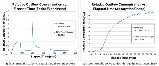
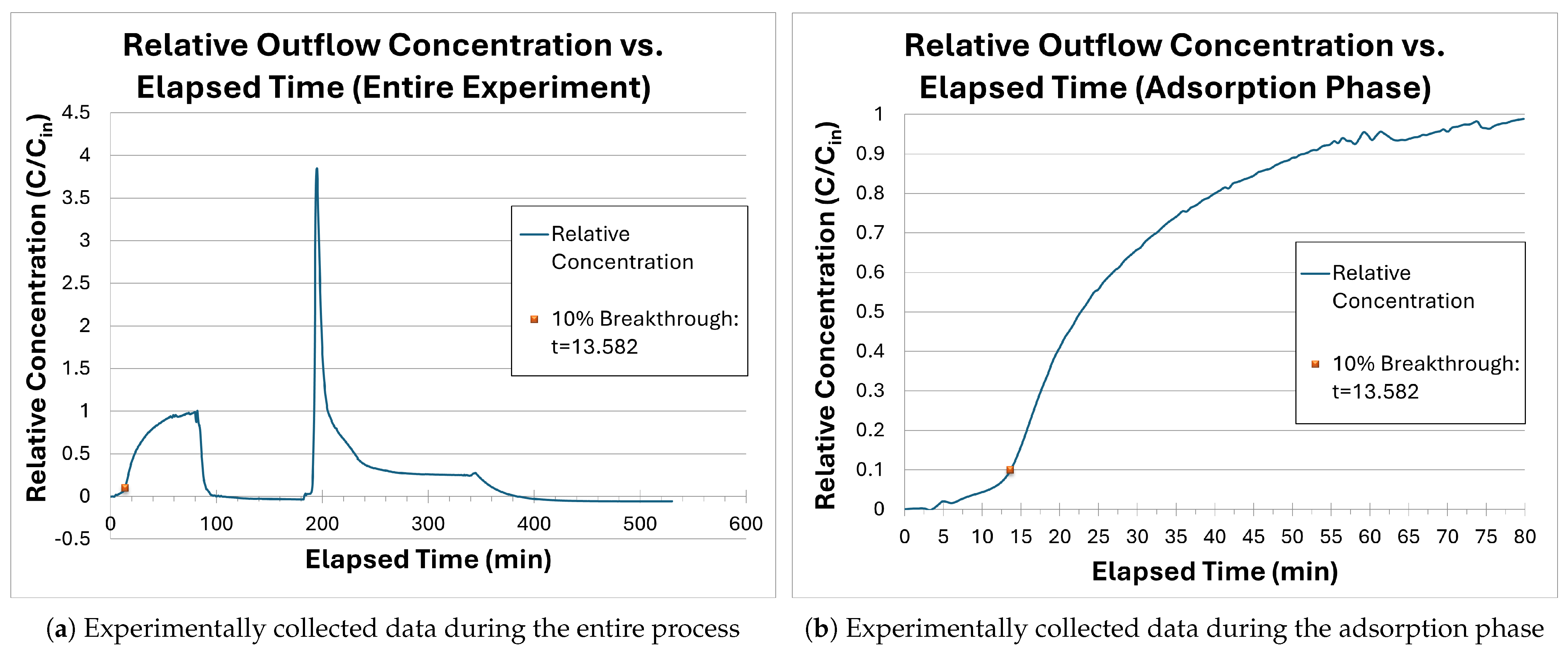
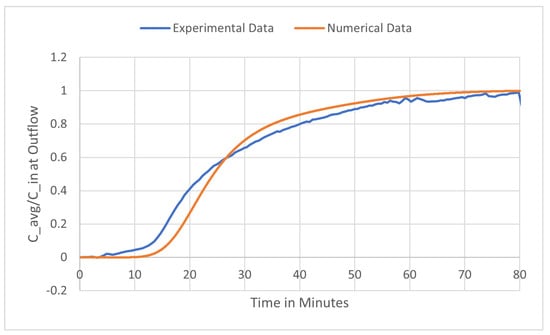
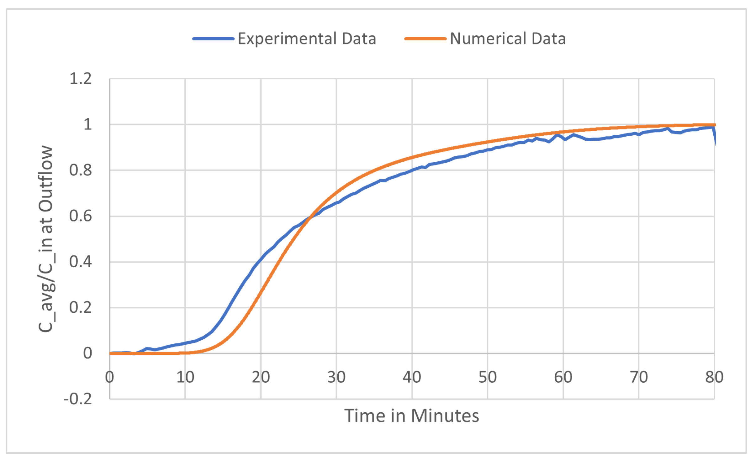
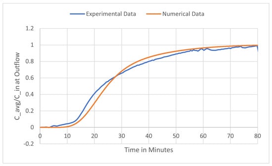
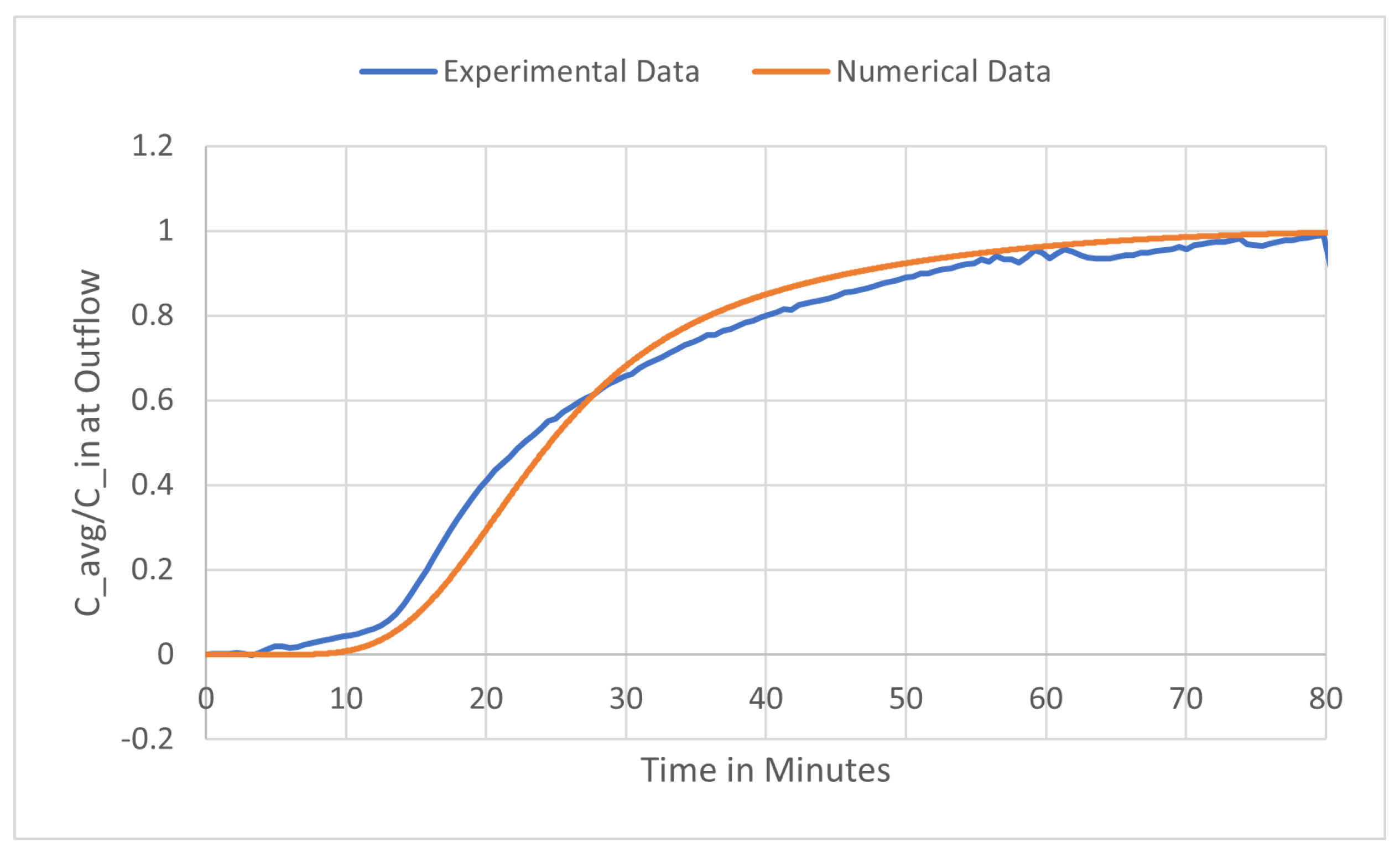
Figure 1a shows the average relative concentration at the outflow through the entire experiment, including all three phases: adsorption, wash, and elution. The average relative concentration is computed by $C/C_{in}$ and gives the dimensionless relative concentration at the outflow. We note that the first peak in the curve is the adsorption front while the second peak corresponds to the elution of the adsorbed protein. This is entirely expected behavior for a preparative membrane chromatography experiment. The adsorption phase (Figure 1b), which is the sole focus of this paper, is the initial sigmoid-shaped curve.

Figure 1. Experimental breakthrough curve data.

An objective of this research is to minimize the difference between data obtained from numerical solution methods and data gathered from experimentation. Because running live experiments can be costly and time-consuming, an accurate simulation will save both time and resources when considering how the experiment will behave under different circumstances. We will refer to the data collected during the live experiment as experimental data and the data obtained from the numerical solution methods as numerical data. For this paper, we will only consider the period of the experiment where the proteins are being adsorbed, the loading or adsorption stage, which is illustrated in Figure 1b.

3. Materials and Methods

This section describes the computational methods and software tools used to obtain numerical solutions to the transport equation modeling of the adsorption phase of the membrane chromatography process. This work focuses exclusively on the adsorption (loading) phase; the wash and elution stages are outside the scope of the present study. We employed FEniCS (FEniCS v2019.1.0, https://fenicsproject.org/) [22], an open-source software package that utilizes finite element methods to solve partial differential equations (PDEs). Finite element methods (FEMs) approximate solutions using piecewise polynomial functions defined on a mesh of the computational domain [23]. These methods offer several advantages: they systematically handle general domains and boundary conditions while maintaining numerical stability [23], and they have been extensively applied in engineering disciplines, including structural analysis in civil engineering and circuit network modeling in electrical engineering [24]. In this section, we describe our implementation of FEniCS to solve the transport Equation (1).

3.1. Weak Formulations

To derive the weak formulation, we multiply both sides of (1) by a test function $v\in V$ and integrate over the domain to obtain

$${\int }_{\mathrm{\Omega }}\left(\omega {\displaystyle \frac{\partial C}{\partial t}}+(1-\omega ){\rho }_s{\displaystyle \frac{\partial q}{\partial t}}+\nabla ·\left(\mathbf{u}C\right)-\nabla ·(\mathbf{D}\nabla C)\right)vd\mathbf{x}={\int }_{\mathrm{\Omega }}fvd\mathbf{x}\forall v\in V,$$

(6)

where $V=\{v\in H^1\left(\mathrm{\Omega }\right):v=0\mathrm{on}{\mathrm{\Gamma }}_D\}$ is the function space for the liquid-phase concentration C, and $W=\{q\in L^2\left(\mathrm{\Omega }\right)\}$ is the function space for the solid-phase concentration q [4,14,15].

Recall that $L^2\left(\mathrm{\Omega }\right)$ is the Lebesgue space of square-integrable functions with associated norm ${\parallel ·\parallel }_2={\left({\int }_{\mathrm{\Omega }}{|·|}^{2}d\mathbf{x}\right)}^{1/2}$ [25]. The Sobolev space $W^{m,p}\left(\mathrm{\Omega }\right)$ consists of functions in $L^p\left(\mathrm{\Omega }\right)$ with weak derivatives up to order m. In particular, when $p=2$ and $m=1$, we obtain the Hilbert space $H^1\left(\mathrm{\Omega }\right)$ with associated norm ${\parallel ·\parallel }_{H^1\left(\mathrm{\Omega }\right)}={\left({\parallel ·\parallel }_2^2+{\parallel \nabla ·\parallel }_2^2\right)}^{1/2}$ [13,26].

We approximate each time derivative using the backward Euler method. The isotherm q requires additional treatment due to its dependence on C in the explicit case and on both C and q in the implicit case. For Langmuir’s isotherm (2), we apply the chain rule to evaluate ${\displaystyle \frac{\partial q}{\partial t}}$ as follows:

$${\displaystyle \frac{\partial q}{\partial t}}={\displaystyle \frac{\partial q}{\partial C}}{\displaystyle \frac{\partial C}{\partial t}}={\displaystyle \frac{(1+k_{2}C)k_1-k_1{k}_{2}C}{{(1+k_{2}C)}^2}}{\displaystyle \frac{\partial C}{\partial t}}={\displaystyle \frac{k_1}{{(1+k_{2}C)}^2}}{\displaystyle \frac{\partial C}{\partial t}}.$$

Applying a lagged backward Euler approximation to ${\displaystyle \frac{\partial C}{\partial t}}$ yields

$${\displaystyle \frac{\partial q}{\partial t}}\approx {\displaystyle \frac{k_1}{{(1+k_2{C}^{n-1})}^2}}{\displaystyle \frac{C^n-C^{n-1}}{\Delta t}}.$$

Combining this approximation with integration by parts, the weak formulation with Langmuir’s isotherm reduces to a problem with one unknown: find $C\in V$ such that

$$\begin{array}{cc}\hfill & {\int }_{\mathrm{\Omega }}\left(\omega +(1-\omega ){\rho }_s{\displaystyle \frac{k_1}{{(1+k_2{C}^{n-1})}^2}}\right){\displaystyle \frac{C^n}{\Delta t}}vd\mathbf{x}-{\int }_{\mathrm{\Omega }}\mathbf{u}{C}^n·\nabla vd\mathbf{x}\hfill \\ \hfill & +{\int }_{\partial \mathrm{\Omega }}\mathbf{u}{C}^n·\mathbf{n}vds+{\int }_{\mathrm{\Omega }}\mathbf{D}\nabla C^n·\nabla vd\mathbf{x}-{\int }_{\partial \mathrm{\Omega }}\mathbf{D}\nabla C^n·\mathbf{n}vds\hfill \\ \hfill & ={\int }_{\mathrm{\Omega }}fvd\mathbf{x}+{\int }_{\mathrm{\Omega }}\left(\omega +(1-\omega ){\rho }_s{\displaystyle \frac{k_1}{{(1+k_2{C}^{n-1})}^2}}\right){\displaystyle \frac{C^{n-1}}{\Delta t}}vd\mathbf{x}\hfill \end{array}$$

(7)

for all $v\in V$.

For the implicitly defined isotherm, we lag q in time by evaluating $q^n=h(C^{n-1},q^{n-1})$ and then approximate ${\displaystyle \frac{\partial q}{\partial t}}$ using a lagged backward Euler difference:

$${\displaystyle \frac{\partial q}{\partial t}}={\displaystyle \frac{q^n-q^{n-1}}{\Delta t}}={\displaystyle \frac{h(q^{n-1},C^{n-1})-h(q^{n-2},C^{n-2})}{\Delta t}}.$$

The weak formulation for Nfor’s isotherm is then as follows: find $(C,q)\in V\times W$ such that

$$\begin{array}{cc}\hfill & {\int }_{\mathrm{\Omega }}\omega {\displaystyle \frac{C^n}{\Delta t}}vd\mathbf{x}-{\int }_{\mathrm{\Omega }}\mathbf{u}{C}^n·\nabla vd\mathbf{x}+{\int }_{\partial \mathrm{\Omega }}\mathbf{u}{C}^n·\mathbf{n}vds\hfill \\ \hfill & +{\int }_{\mathrm{\Omega }}\mathbf{D}\nabla C^n·\nabla vd\mathbf{x}-{\int }_{\partial \mathrm{\Omega }}\mathbf{D}\nabla C^n·\mathbf{n}vds\hfill \\ \hfill & ={\int }_{\mathrm{\Omega }}fvd\mathbf{x}+{\int }_{\mathrm{\Omega }}\left(\omega {\displaystyle \frac{C^{n-1}}{\Delta t}}-(1-\omega ){\rho }_s{\displaystyle \frac{q^n-q^{n-1}}{\Delta t}}\right)vd\mathbf{x}\hfill \end{array}$$

(8)

for all $v\in V$.

3.2. FEniCS Implementation

To implement a finite element method, we first discretize the spatial domain to obtain the mesh on which our equation will be solved. In this work, we employ a two-dimensional rectangular mesh to represent the porous medium in the chromatography column. Using FEniCS’s built-in functions, we define the mesh with the desired discretization via the command:

• mesh=RectangleMesh("lower left point","upper right point",nx,ny)

where nx and ny denote the number of mesh points along the x- and y-axes, respectively.

The function space V is then defined on the mesh using built-in functions, along with the trial function $C^n$ and test function v. We define a piecewise quadratic Lagrange element space:

• V = FunctionSpace(mesh,’P’,2)
• C_n = TrialFunction(V)
• v = TestFunction(V)

For the initial condition $C(\mathbf{x},0)=C_0=0$, we interpolate the zero function over the entire mesh and compute $q(\mathbf{x},0)=q_0$ using $C_0$. Each of the four boundaries is identified and labeled with boundary markers using different classes. For example,

• class bound_inflow(SubDomain):
•   def inside(self,x,on_boundary):
•      return on_boundary and near(x[1], height)
• b_top=bound_inflow()
• b_top.mark(boundary_markers,0)

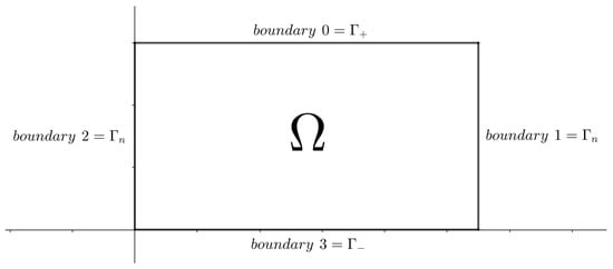
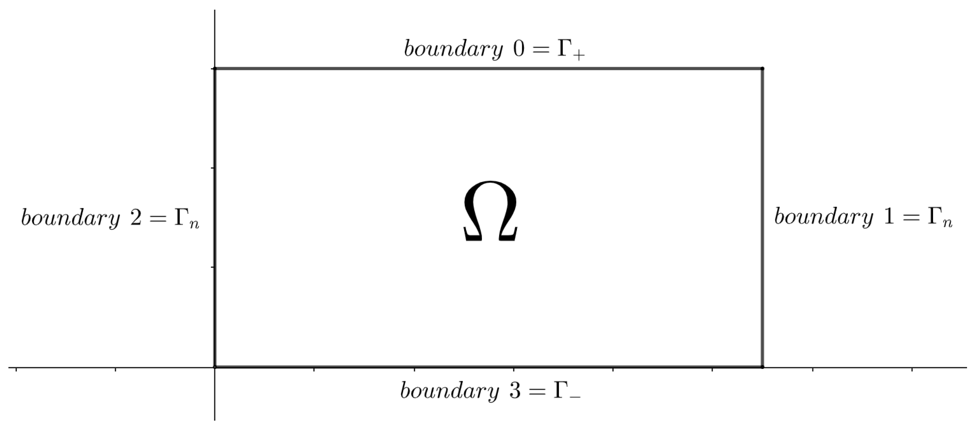
The four boundaries are labeled 0 through 3, as shown in Figure 2.

Figure 2. Boundary labeling of the defined mesh.

On the boundary ${\mathrm{\Gamma }}_{+}$, we prescribe a parabolic concentration profile with zero concentration at the lateral boundaries and average value equal to the experimental concentration $C_{exp}$:

$$C_{in}=C_{exp}{\displaystyle \frac{6x(x-\mathrm{width})}{{\mathrm{width}}^2}}.$$

The parabolic concentration profile is chosen to be consistent with the distribution of concentration in unobstructed flow through a pipe. This Dirichlet condition is defined using FEniCS’s built-in function with the previously defined boundary marker:

• bc=DirichletBC(V,C_in,b_top)

Since $(\mathbf{u}-\mathbf{D}\nabla C)·\mathbf{n}(\mathbf{x},t)=0$ on ${\mathrm{\Gamma }}_n$, we do not evaluate the boundary integrals when $\mathbf{x}\in {\mathrm{\Gamma }}_n$. Along ${\mathrm{\Gamma }}_{-}$, we weakly impose the boundary condition $\nabla C·\mathbf{n}=0$ and evaluate the corresponding boundary integral along the outflow boundary. For simplicity and computational efficiency, we set $\Delta t=h=0.05$ for all implementations. We note that smaller values may reduce numerical error; however, our choice significantly reduces computational time, particularly for iterative optimization methods, and ensures consistent comparisons across simulations.

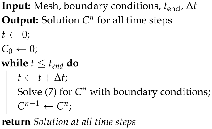
We note that additional steps are required to discretize the equation in time [27]. While FEniCS does not provide built-in time discretization, the implementation is straightforward. We enclose the code for solving the equation within a loop that solves for one time step, stores the solution, advances time, and repeats until the desired final time is reached. The algorithm for solving the time-discretized weak formulations with Langmuir’s isotherm given by (7) is shown in Algorithm 1.

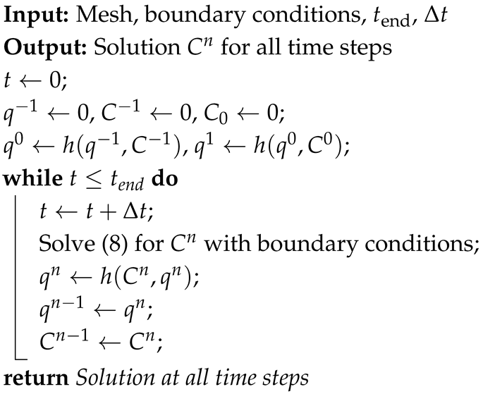
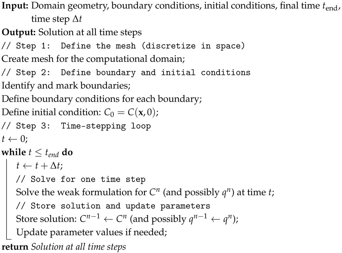
In the weak formulation with Nfor’s isotherm, we initialize $q^{-1}=0$, $C_0=0$, and $C^{-1}=0$ for the first time step, which yields $q^0=h(q^{-1},C^{-1})$ and $q^1=h(q^0,C^0)$. After solving for the first time step, we update $q^2=h(q^1,C^1)$, and this pattern continues for all subsequent time steps. The algorithm for solving time-discretized weak formulations with Nfor’s isotherm given by (8) is shown in Algorithm 2. Algorithm 3 presents a general algorithm for solving a time-dependent PDE in FEniCS.   

Algorithm 1: Transport equation with Langmuir’s isotherm

Algorithm 2: Transport equation with Nfor’s isotherm

Algorithm 3: General FEniCS implementation for time-dependent PDEs

3.3. Initial Numerical Results

For comparison with experimental data, we initially chose parameter values to replicate the associated laboratory conditions described in Section 2. The isotherm parameter values were obtained through data fitting methods described in [11]. As described in Section 3.2, we use initial conditions of $C_0$ and $q_0$ and set both to 0; this models no protein concentration in the column initially.

As described in Section 2, we assumed a time-independent velocity profile since the flow rate in the chromatography column was constant. The vertical velocity was chosen to have a parabolic profile with zero velocity at the lateral boundaries and maximum velocity chosen to ensure the correct flow rate; the parabolic velocity profile was chosen to coincide with unobstructed flow through a pipe. The horizontal velocity was assumed to be zero.

Diffusion coefficients of protein molecules in porous membranes range from $6\times {10}^{-4}$ cm²/min for small proteins such as glycine to $2.28\times {10}^{-5}$ cm²/min for large proteins such as immunoglobulin G (IgG) [28]. We chose a diffusion coefficient of $D=2.28\times {10}^{-5}$ cm²/min, corresponding to IgG used in the experiment. The mean microscopic velocity $\left|\mathbf{u}\right|$ was approximated from the constant flow rate of 0.1 mL/min:

$$\left|\mathbf{u}\right|\approx {\displaystyle \frac{\mathrm{flow}\mathrm{rate}}{\pi r^2}}=0.0497\mathrm{cm}/\min .$$

The longitudinal and transverse dispersivities, ${\alpha }_L$ and ${\alpha }_T$, are known to vary widely depending on the physical properties of the membrane. Experimental values for ${\alpha }_L$ at small scales range from a few millimeters to nearly one hundred centimeters, depending on porosity [20,29], with ${\alpha }_L$ decreasing as porosity increases [30]. Since our porosity is close to unity, ${\alpha }_L$ should be on the lower end of this range, on the order of a few millimeters. Additionally, ${\alpha }_T$ is generally found to be between ${\displaystyle \frac{1}{5}}$ and ${\displaystyle \frac{1}{100}}$ of ${\alpha }_L$ [20]. Initial visual comparison of experimental and numerical breakthrough curves indicated that ${\alpha }_T={\displaystyle \frac{1}{10}}{\alpha }_L$ produced curves with similar shapes. The initial value of ${\alpha }_L=1.37$ was chosen to match the experimental and numerical points of 10% breakthrough. Throughout the remainder of this paper, we use the variable μ to denote the coefficient in the relation ${\alpha }_T=\mu {\alpha }_L$ for simplicity.

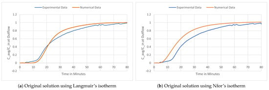
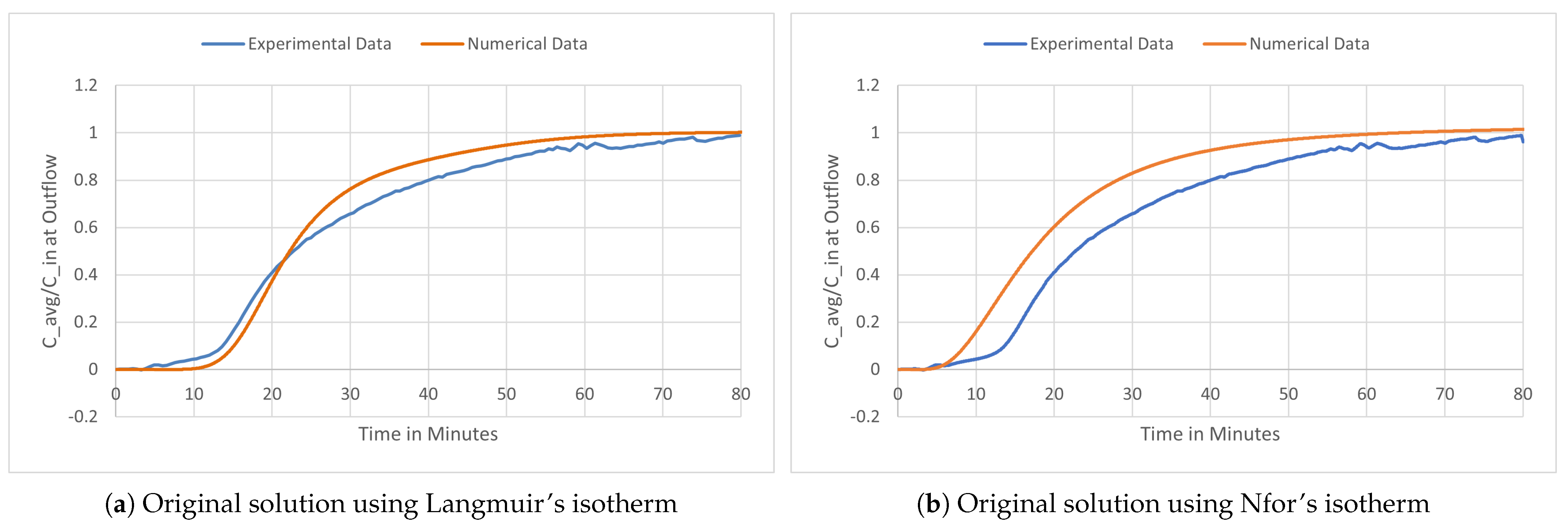
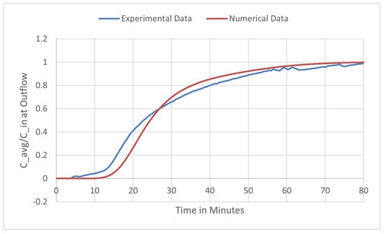
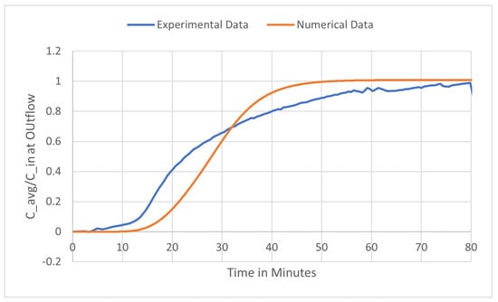
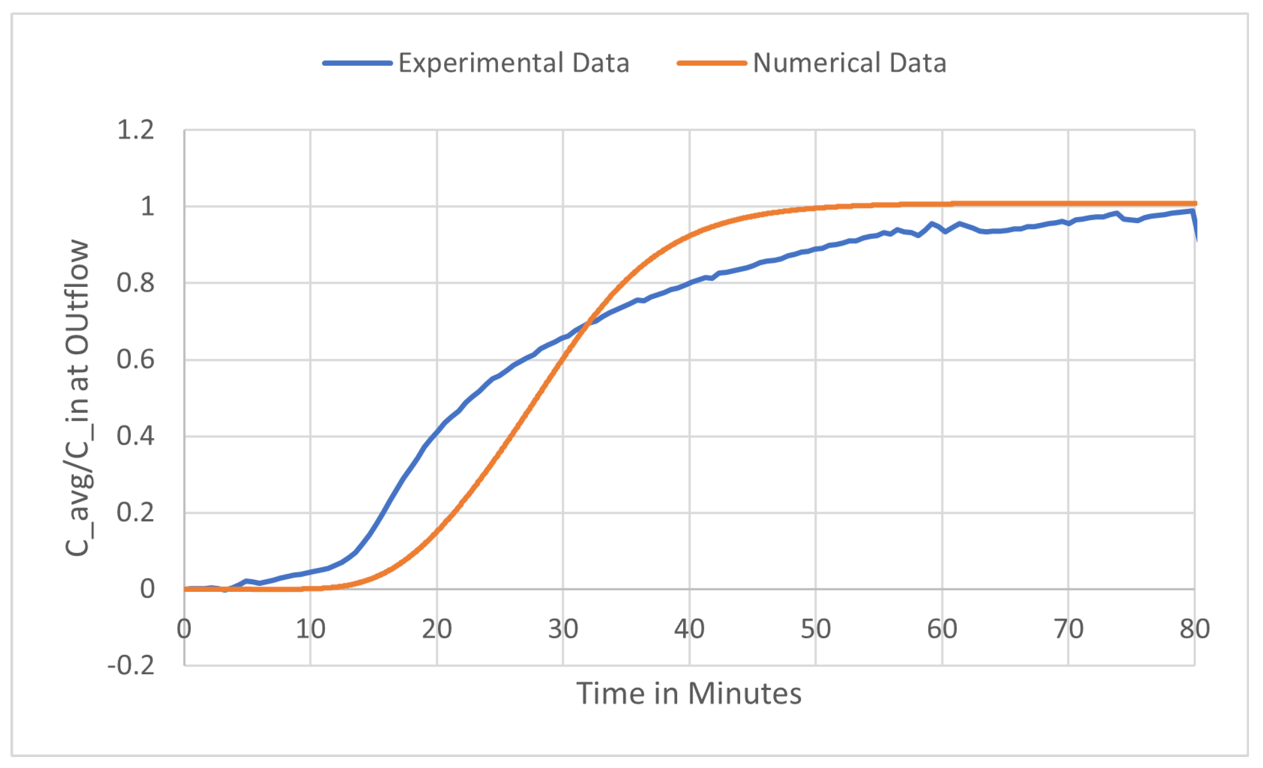
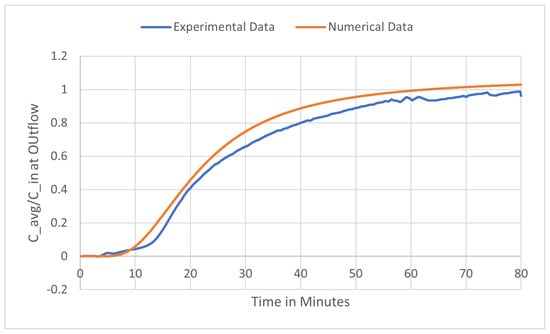
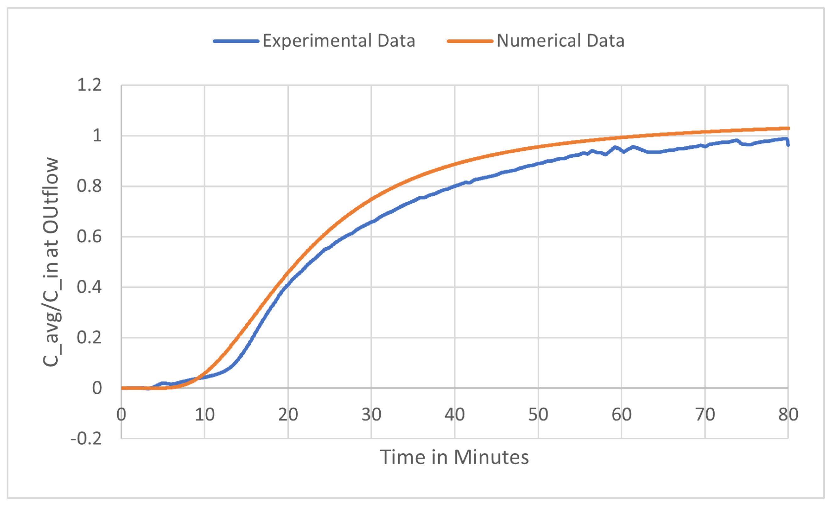
All parameters have inherent uncertainty, and we investigate the effects of this uncertainty on the model solution in subsequent sections. Figure 3a shows the initial results using Langmuir’s isotherm with parameter values given in Table 1. The numerical results using Nfor’s isotherm with its original parameter values, given in Table 2, are shown in Figure 3b.

Figure 3. Initial numerical results with original parameter values.

Table 1. Original parameter values for Langmuir’s isotherm. Units are given beside each parameter; (-) indicates the parameter is unitless.

$\mathit{\omega }$ (-)	${\mathit{\alpha }}_{\mathit{L}}$ (cm)	$\mathit{\mu }$ (-)	${\mathit{\rho }}_{\mathit{s}}$ (mg/mL)	${\mathit{k}}_{\mathit{eq}}$ (mL/mg)	${\mathit{q}}_{\mathit{max}}$ (mg/mL)
0.84	1.37	0.1	1	2.06	150

Table 2. Original parameter values for Nfor’s isotherm. Units are given beside each parameter; (-) indicates the parameter is unitless. Note that M denotes Molarity, which is the unit of moles per liter.

$\mathit{\omega }$ (-)	${\mathit{\alpha }}_{\mathit{L}}$ (cm)	$\mathit{\mu }$ (-)	${\mathit{\rho }}_{\mathit{s}}$ (mg/mL)	${\mathit{k}}_{\mathit{eq}}$ (mL/mg)	${\mathit{q}}_{\mathit{max}}$ (mg/mL)	$\mathbf{\Lambda }$ (M)
0.84	1.37	0.1	1	502	216	0.34009
$\mathit{v}$ (-)	$\mathit{r}$ (-)	$\mathit{z}$ (-)	${\mathit{c}}_{\mathit{s}}$ (M)	${\mathit{c}}_{\mathit{m}}$ (M)	${\mathit{k}}_{\mathit{s}}$ (M−1)	${\mathit{k}}_{\mathit{p}}$ (mL/mg)
0.1	1	1	0.37	55.5	$-0.1$	$-0.1$

4. Parameter Investigation

In this section, we investigate each parameter in the transport equation with Langmuir’s isotherm to assess the range over which reasonable agreement with experimental data is maintained. We measure goodness of fit by the area between the experimental and numerical breakthrough curves. Using the parameter values in Table 1 as our baseline, we determine how far each parameter can vary while still producing acceptable results.

4.1. Porosity of the Membrane, $\omega$

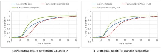
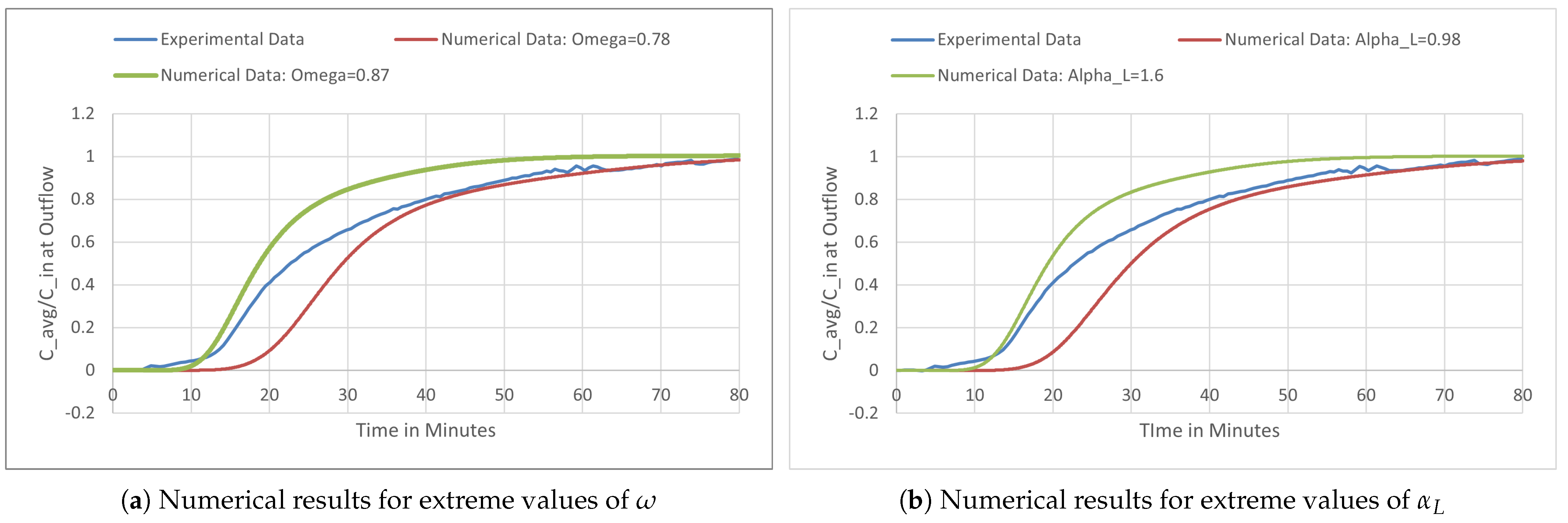
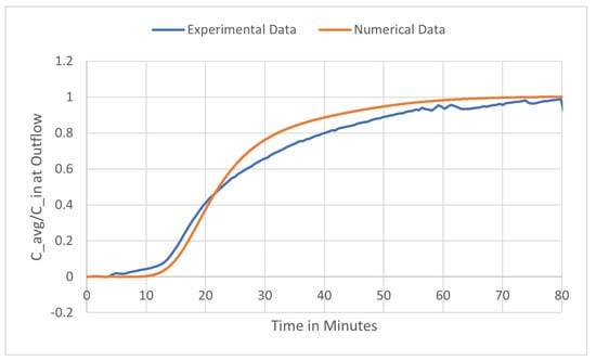
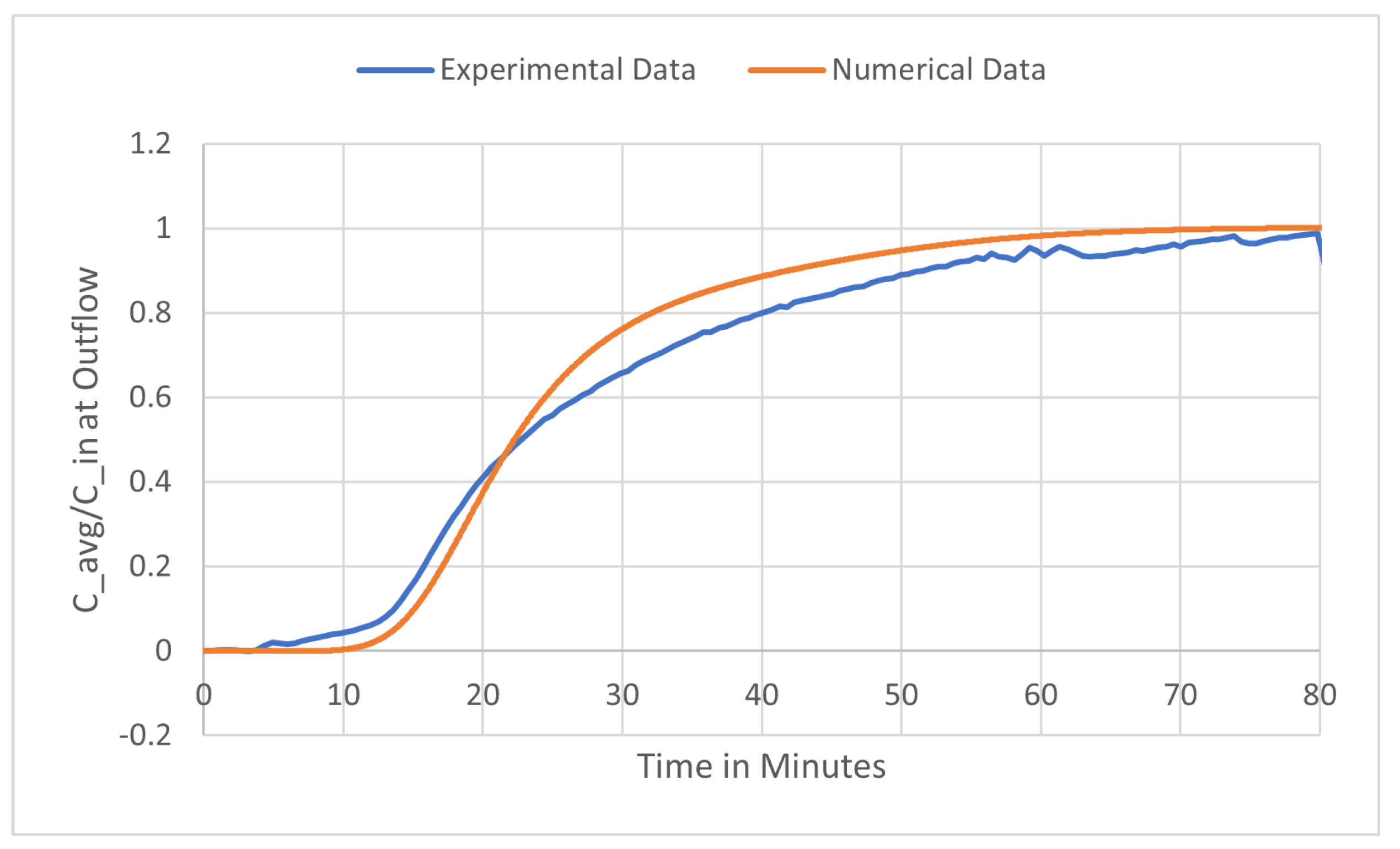
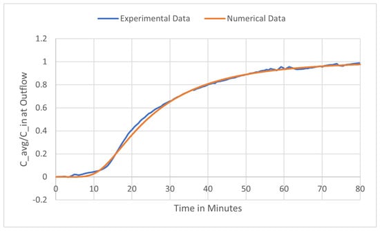
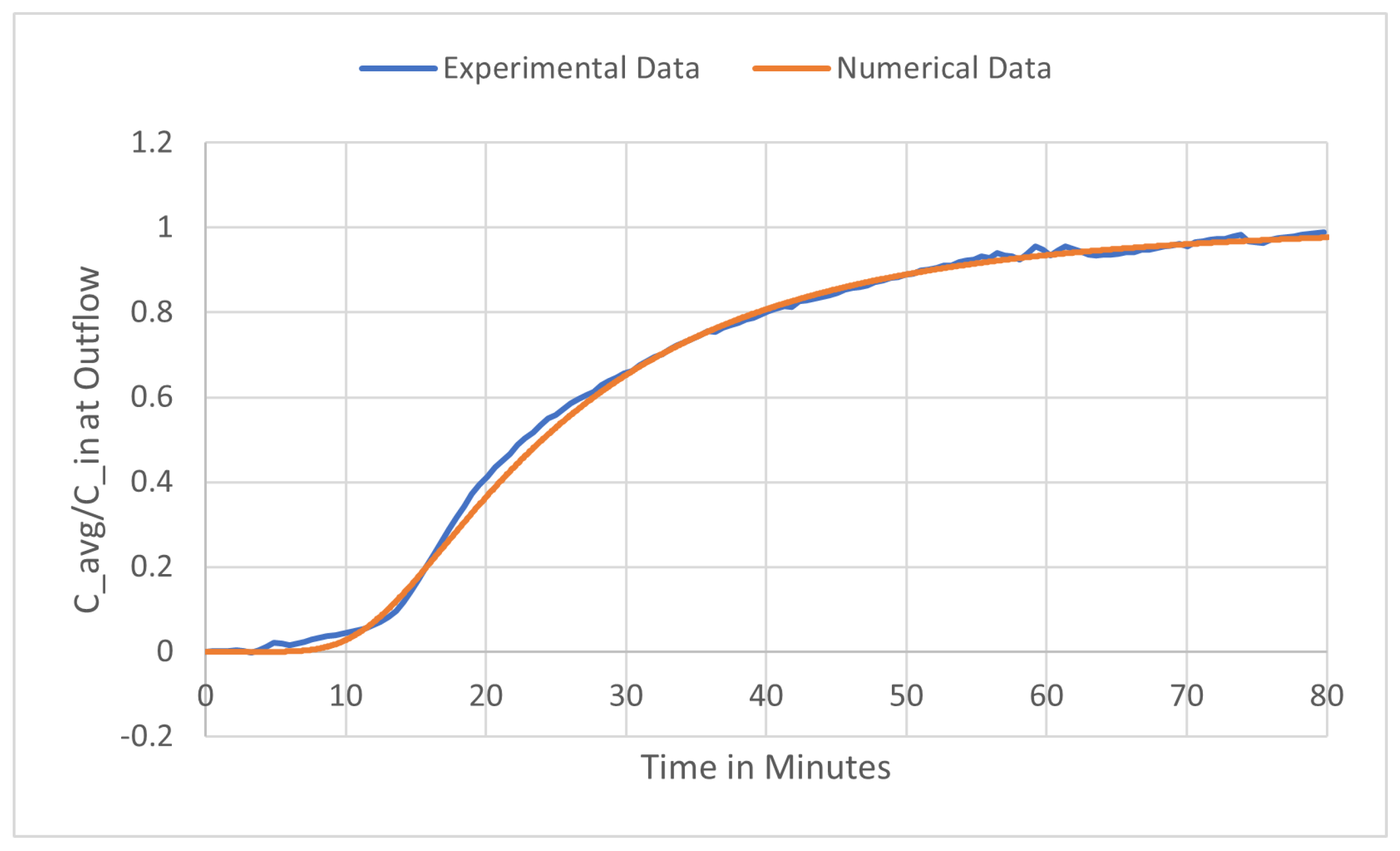
The porosity $\omega$ is defined as the ratio of void volume to total volume. Since $\omega =1$ would imply no solid phase available for protein adsorption, and $\omega =0$ would represent a completely solid medium preventing flow, we have $\omega \in (0,1)$. By varying $\omega$ while holding other parameters fixed at their original values, we find that reasonable agreement with experimental data is obtained for $\omega \in (0.78,0.87)$. Figure 4a shows the numerical results at the bounds of this range compared with experimental data.

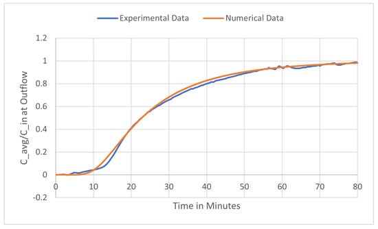
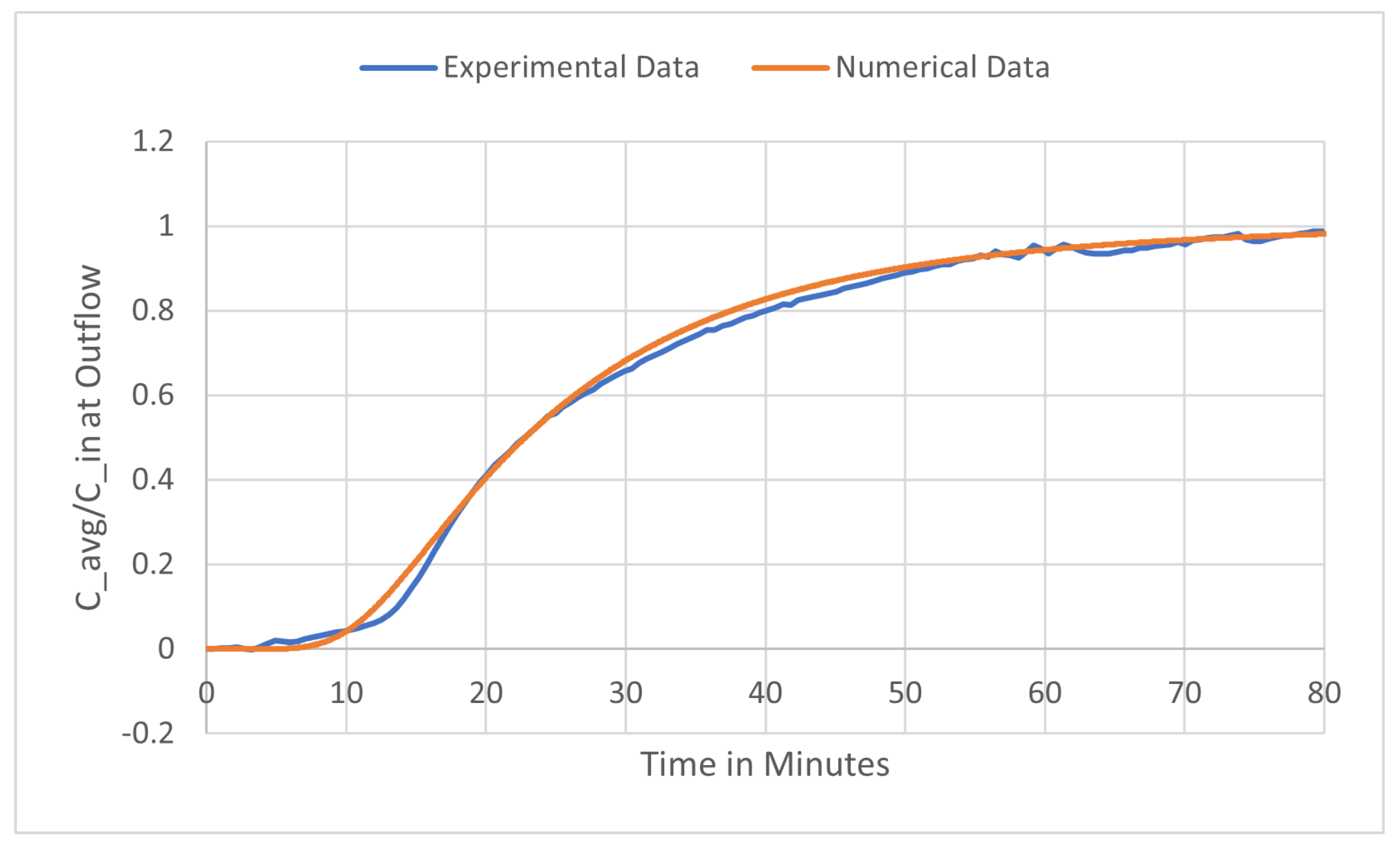
Figure 4. Parameter range investigation for Langmuir’s isotherm, compared with experimental data.

4.2. Longitudinal Dispersivity, ${\alpha }_L$

The longitudinal dispersivity ${\alpha }_L$ is known to vary significantly across different physical systems, ranging from a few centimeters to hundreds of centimeters [20]. Testing multiple values in the neighborhood of ${\alpha }_L=1.37$, we find that ${\alpha }_L\in (0.98,1.6)$ produces reasonable agreement with experimental data. Figure 4b compares the numerical results at these bounds with experimental data.

4.3. Transverse Dispersivity, ${\alpha }_T$

The transverse dispersivity is defined as ${\alpha }_T=\mu {\alpha }_L$, where the coefficient μ typically ranges from ${\displaystyle \frac{1}{100}}$ to ${\displaystyle \frac{1}{5}}$ [4,20]. Through numerical simulations, we observe that variations in μ within this range produce minimal changes in the breakthrough curves. Our investigation indicates that the entire range $\mu \in (0.01,0.2)$ yields acceptable results.

4.4. Summary of Results

Table 3 summarizes the investigated parameter ranges. We emphasize that these ranges represent initial sensitivity analyses in which each parameter is varied individually while others remain fixed. When parameters are varied simultaneously, acceptable results may be obtained for values outside these intervals due to compensating effects among parameters.

Table 3. Initial parameter value ranges for Langmuir’s isotherm. Units are given beside each parameter; (-) indicates the parameter is unitless.

Parameter	Range
$\omega$ (-)	$(0.78,0.87)$
${\alpha }_L$ (cm)	$(0.98,1.6)$
$\mu$ (-)	$(0.01,0.2)$
${\rho }_s$ (mg/mL)	$(0.8,1.35)$
$k_{eq}$ (mL/mg)	$(1,4.757)$
$q_{max}$ (mg/mL)	$(130,205)$

5. Single Parameter Optimization

The goal of the optimization described in this section is to determine parameter values that produce the best agreement with experimental data. To achieve this, we first change only one parameter at a time, and we minimize the difference between the numerical average concentration at the outflow, $c_{(N,avg)}$, and the experimental average concentration at the outflow, $c_{(E,avg)}$.

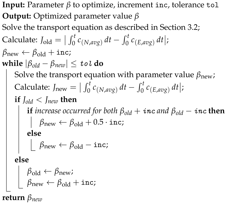
The most widely used objective function for parameter identification is the least squares approach [5,31]. However, since our numerical simulations produce more data points than are available from experiments, we employ an alternative method for the single parameter optimization problem. We approximate the area under both the numerical and experimental breakthrough curves using the trapezoidal rule for numerical integration and minimize the absolute difference via a line search algorithm, optimizing one parameter at a time. The objective function to be minimized is given by

$$J=|{\int }_0^t{c}_{(N,avg)}dt-{\int }_0^t{c}_{(E,avg)}dt|.$$

(9)

Algorithm 4 shows the line search algorithm. We set a tolerance of 0.0001 to provide accuracy to four decimal places for each parameter investigated.

Algorithm 4: Line search for parameter optimization

5.1. Optimizing the Porosity, $\omega$

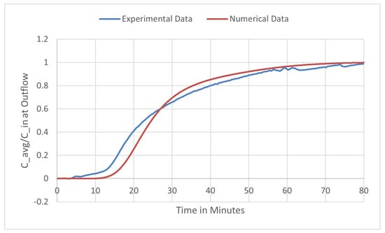
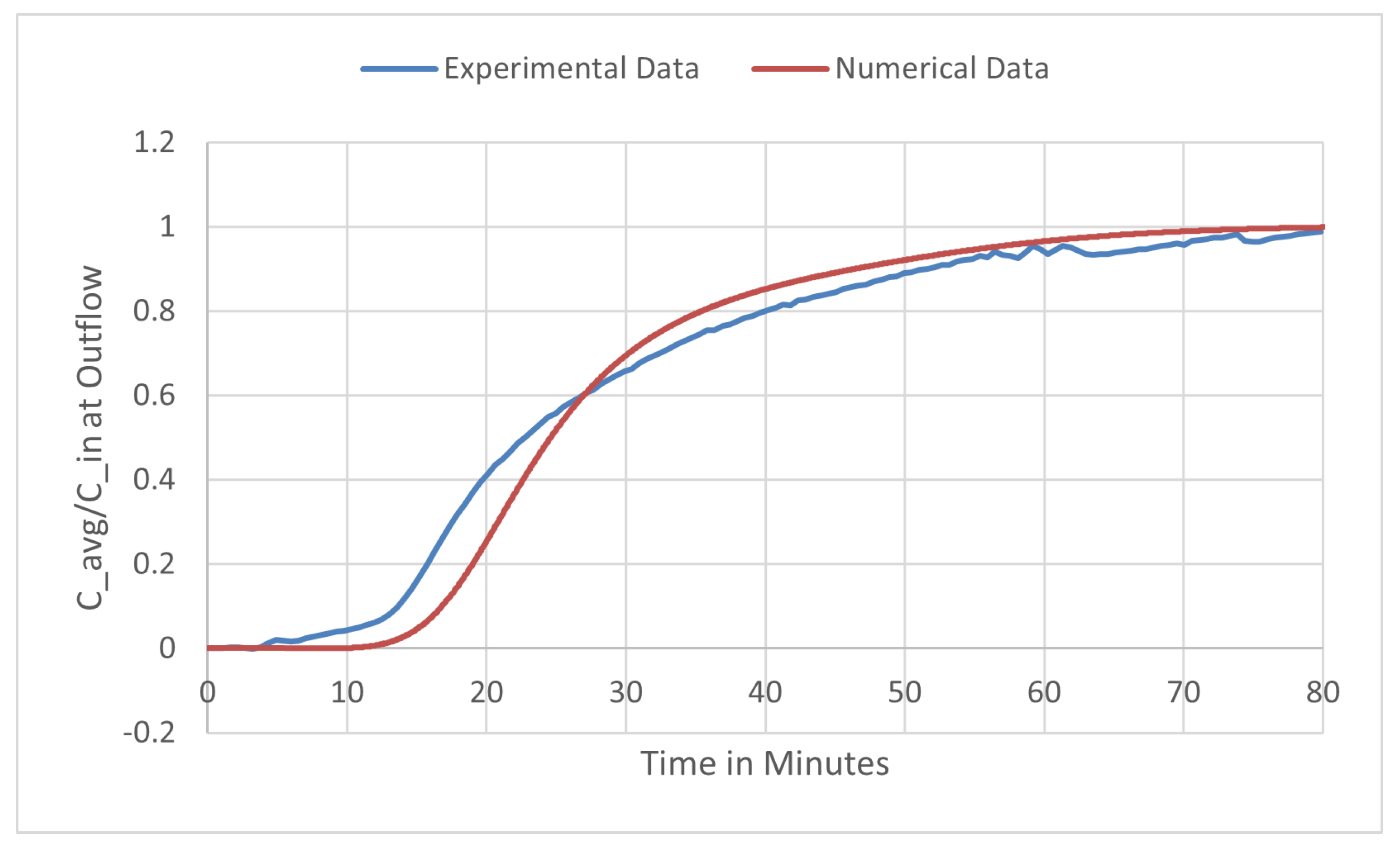
Adjusting $\omega$ corresponds to changing the membrane porosity, thereby altering the available void space for flow. Starting from an initial value of $\omega =0.5$, the line search algorithm converges to a final value of $\omega \approx 0.8203$. Table 4 presents the final iterations of the optimization process, and Figure 5 compares the resulting numerical solution with experimental data.

Table 4. Final iterations of the line search algorithm for $\omega$ with initial value $\omega =0.5$, showing the objective function values for Langmuir’s isotherm. Units are given beside each parameter; (-) indicates the parameter is unitless.

$\mathit{\omega }$ (-)	J (Difference)
0.8125	1.333835
0.75	9.56408
0.875	7.306422
0.84375	2.966926
0.78125	5.534577
0.796875	3.451087
0.828125	0.808823
0.84375	2.966844
0.8125	1.332871
0.820313	0.264482

Figure 5. Comparison of experimental data and numerical results with optimized porosity $\omega =0.8203$.

5.2. Optimizing Longitudinal Dispersivity, ${\alpha }_L$

Optimizing ${\alpha }_L$ adjusts the dispersion tensor, which governs fluid flow through the porous medium, thereby producing solutions that align more closely with experimental data. Since ${\alpha }_T$ is defined as ${\alpha }_T=\mu {\alpha }_L$ with $\mu =0.1$, variations in ${\alpha }_L$ automatically adjust ${\alpha }_T$ proportionally. Table 5 presents the final iterations of the line search algorithm starting from an initial value of ${\alpha }_L=10$.

Table 5. Final iterations of the line search algorithm for ${\alpha }_L$ with initial value ${\alpha }_L=10$, showing objective function values. Units are given beside each parameter.

${\mathit{\alpha }}_{\mathbf{L}}$ (cm)	${\mathit{\alpha }}_{\mathbf{T}}$ (cm)	J (Difference)
1	0.1	5.82730
1.5	0.15	4.49670
1.375	0.1375	2.53326
1.125	0.1125	2.53283
1.1875	0.11875	1.09604
1.3125	0.13125	1.42496
1.28125	0.128125	0.83503
1.21875	0.121875	0.42392
1.234375	0.1234375	0.09890

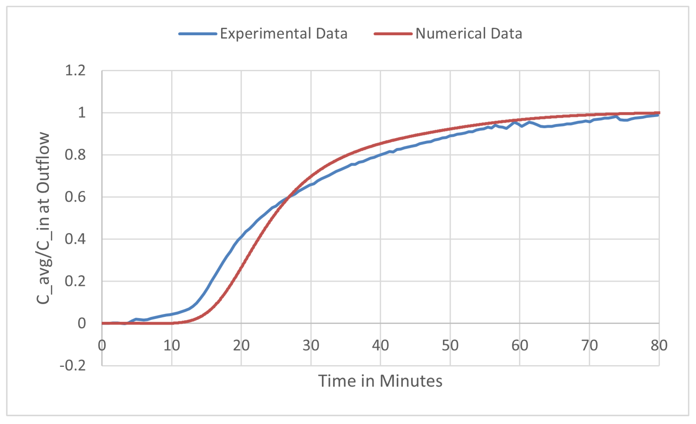
The small final objective function value suggests good agreement. However, visual inspection of Figure 6 reveals a discrepancy: the experimental data exhibits a slower initial rise in outlet concentration compared to the numerical results. This highlights a fundamental limitation of the area-based objective function (9).

Figure 6. Comparison of numerical results with optimized ${\alpha }_L=1.2344$ and experimental data for Langmuir’s isotherm.

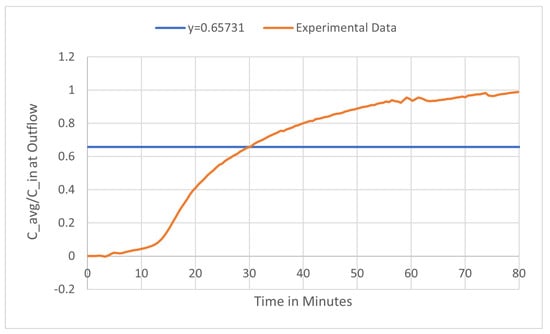
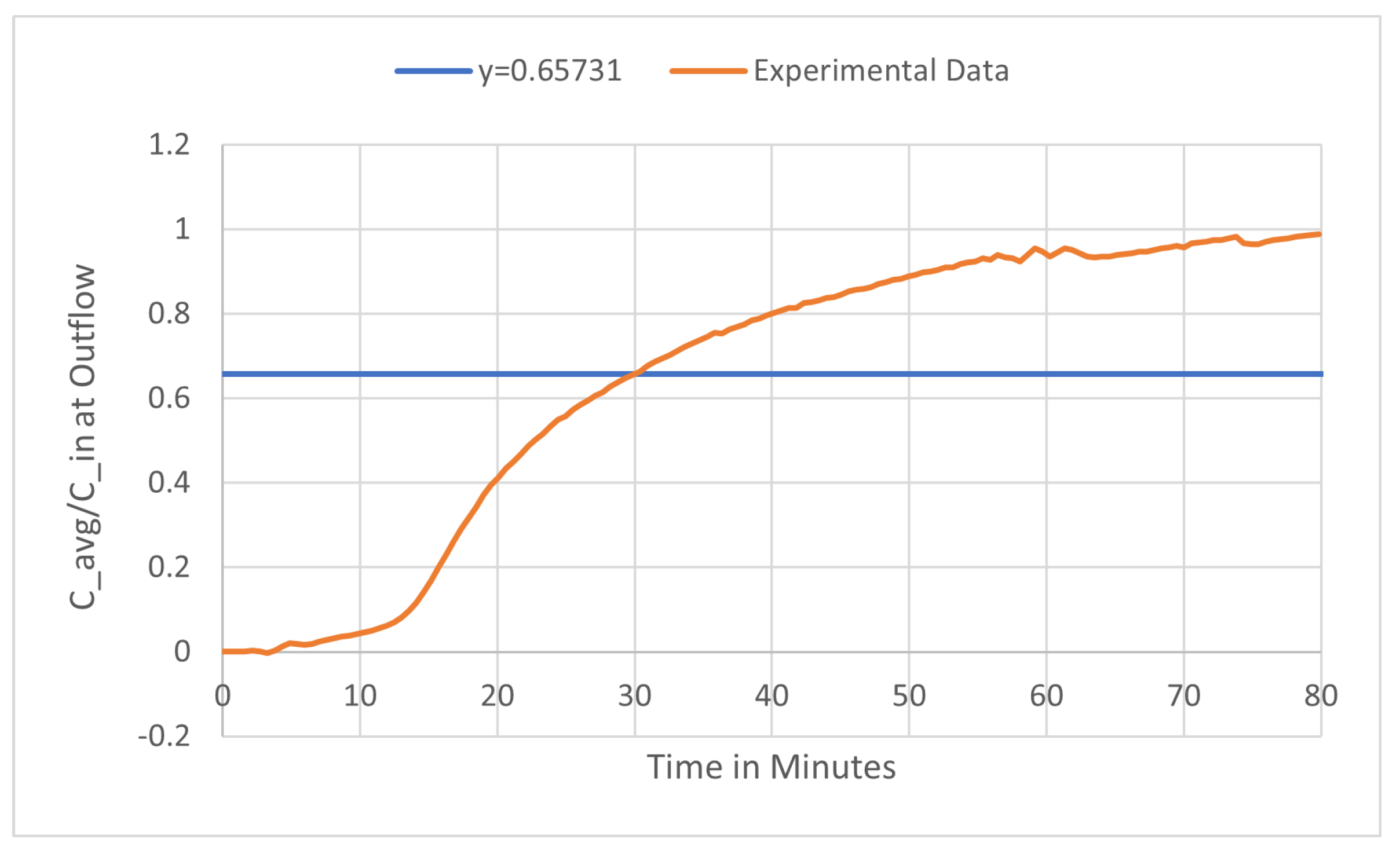
To illustrate this issue, consider a geometric analogy: a triangle with base 2 and height 4 has the same area (4 square units) as a rectangle with base 2 and height 2, yet the shapes are visually distinct. Similarly, different breakthrough curve shapes can yield identical areas. Figure 7 demonstrates an extreme case where setting $C_{(avg,n)}/C_{in}=0.65731$ for all times t produces the same area as the experimental data despite clearly being an inaccurate solution.

Figure 7. Example demonstrating the limitation of area-based optimization: constant value $C_{(avg,n)}/C_{in}=0.65731$ yields identical area but poor fit to experimental data.

We investigated several larger initial values for ${\alpha }_L$, which also produced small area differences but exhibited poor visual agreement with experimental breakthrough curves. This analysis demonstrates that while the area-based objective function provides a useful optimization metric, it must be supplemented with visual inspection to ensure physically meaningful solutions.

5.3. Sequential Single-Parameter Optimization

We applied the optimization technique described in Section 5 sequentially to each parameter. The first optimization sequence investigated was $\omega$, ${\alpha }_L$, ${\rho }_s$, $k_{eq}$, $q_{max}$, with ${\alpha }_T$ maintained at one-tenth of ${\alpha }_L$ (i.e., $\mu =0.1$). We chose to optimize $\omega$ first because experimental measurements indicated that manufacturer-reported membrane porosity values can be inaccurate by as much as 20% relative difference. Figure 8 compares the experimental and numerical results, with optimized parameter values listed in Table 6. The optimized value for $\omega$ differs from the original by only 0.0178, while ${\alpha }_L$ differs by 0.0003. Both the parameter changes and the objective function value remain relatively small.

Figure 8. Sequential line search results for Langmuir’s isotherm with optimization order $\omega$, ${\alpha }_L$, ${\rho }_s$, $k_{eq}$, $q_{max}$.

Table 6. Optimized parameter values for Langmuir’s isotherm with sequential optimization order $\omega$, ${\alpha }_L$, ${\rho }_s$, $k_{eq}$, $q_{max}$. Units are given beside each parameter; (-) indicates the parameter is unitless.

Parameter	Value
$\omega$ (-)	0.8222
${\alpha }_L$ (cm)	1.3703
$\mu$ (-)	0.1
${\rho }_s$ (mg/mL)	0.9999
$k_{eq}$ (mL/mg)	2.0600
$q_{max}$ (mg/mL)	150.0154

We also investigated alternative optimization sequences: ${\alpha }_L$, $\omega$, ${\rho }_s$, $k_{eq}$, $q_{max}$ (Table 7 and Figure 9) and ${\rho }_s$, ${\alpha }_L$, $\omega$, $k_{eq}$, $q_{max}$ (Table 8 and Figure 10). Table 9 compares the final objective function values for each optimization sequence. The largest difference, approximately 0.5965 units squared, occurs for the third sequence, demonstrating that optimization order significantly affects the results.

Table 7. Optimized parameter values for Langmuir’s isotherm with sequential optimization order ${\alpha }_L$, $\omega$, ${\rho }_s$, $k_{eq}$, $q_{max}$. Units are given beside each parameter; (-) indicates the parameter is unitless.

Parameter	Value
$\omega$ (-)	0.8400
${\alpha }_L$ (cm)	1.2391
$\mu$ (-)	0.1
${\rho }_s$ (mg/mL)	1.1085
$k_{eq}$ (mL/mg)	1.2256
$q_{max}$ (mg/mL)	150.0029

Figure 9. Sequential line search results for Langmuir’s isotherm with optimization order ${\alpha }_L$, $\omega$, ${\rho }_s$, $k_{eq}$, $q_{max}$.

Table 8. Optimized parameter values for Langmuir’s isotherm with sequential optimization order ${\rho }_s$, ${\alpha }_L$, $\omega$, $k_{eq}$, $q_{max}$. Units are given beside each parameter; (-) indicates the parameter is unitless.

Parameter	Value
$\omega$ (-)	0.8222
${\alpha }_L$ (cm)	1.3699
$\mu$ (-)	0.1
${\rho }_s$ (mg/mL)	0.9999
$k_{eq}$ (mL/mg)	2.0599
$q_{max}$ (mg/mL)	149.9707

Figure 10. Sequential line search results for Langmuir’s isotherm with optimization order ${\rho }_s$, ${\alpha }_L$, $\omega$, $k_{eq}$, $q_{max}$.

Table 9. Objective function values for different parameter optimization sequences using Langmuir’s isotherm.

Parameter Optimization Order	J (Difference)
$\omega$, ${\alpha }_L$, ${\rho }_s$, $k_{eq}$, $q_{max}$	0.0250
${\alpha }_L$, $\omega$, ${\rho }_s$, $k_{eq}$, $q_{max}$	0.0247
${\rho }_s$, ${\alpha }_L$, $\omega$, $k_{eq}$, $q_{max}$	0.5965

The order dependence observed here reflects a deeper issue of parameter coupling and practical identifiability. Several parameters in the transport equation have compensating effects on the breakthrough curve shape. When parameters are estimated sequentially, the value found for an early parameter absorbs some of the effect that a later parameter would otherwise correct, leaving the later optimization with a reduced range of improvement. This is a known limitation of sequential single-parameter approaches in inverse problems, and it motivates the simultaneous multi-parameter optimization developed in Section 6, where the gradient-based adjoint method accounts for the coupled dependence of the objective function on all parameters at once.

Note that the final objective function values are generally similar across different optimization sequences. However, as discussed in Section 5.2, many different curves can yield identical areas while having vastly different shapes. This necessitates visual inspection of the breakthrough curves in addition to numerical assessment of the objective function.

In the previous examples, we fixed ${\alpha }_T=0.1{\alpha }_L$. To verify whether this represents the optimal relationship, we extended the optimization sequences to include μ as a variable parameter in ${\alpha }_T=\mu {\alpha }_L$. We found that obtaining reasonable solutions requires initializing μ close to its original value, suggesting that μ may be a highly sensitive parameter. Table 10 and Figure 11 present the results for the optimization sequence ${\alpha }_L$, $\mu$, $\omega$, ${\rho }_s$, $q_{max}$, $k_{eq}$.

Table 10. Optimized parameter values for Langmuir’s isotherm with sequential optimization order ${\alpha }_L$, $\mu$, $\omega$, ${\rho }_s$, $q_{max}$, $k_{eq}$. Units are given beside each parameter; (-) indicates the parameter is unitless.

Parameter	Value
$\omega$ (-)	0.856
${\alpha }_L$ (cm)	1.3699
$\mu$ (-)	0.099
${\rho }_s$ (mg/mL)	1.1085
$k_{eq}$ (mL/mg)	2.0599
$q_{max}$ (mg/mL)	150.0054

Figure 11. Sequential line search results for Langmuir’s isotherm with optimization order ${\alpha }_L$, $\mu$, $\omega$, ${\rho }_s$, $q_{max}$, $k_{eq}$.

While Figure 11 shows the closest agreement with experimental data during the first 20 time steps, significant discrepancies emerge in the middle portion of the simulation before converging again near the end. This optimization sequence yields an objective function value of 1.9381, which is substantially larger than the values in Table 9.

These results demonstrate that different parameter optimization sequences can yield substantially different outcomes. We conclude that sequential single-parameter optimization introduces order-dependent sensitivity among parameters. This motivates the need for a simultaneous multi-parameter optimization method to ensure globally optimal results.

6. Multi-Parameter Optimization

The FEniCS program utilizes the dolfin package for numerical computations. Through an additional package, dolfin-adjoint, we can employ built-in optimization methods to optimize multiple parameters simultaneously. This section discusses the implementation and compares several built-in optimization methods.

Optimization methods typically use gradient calculations to determine either a tangent line at a particular point or a direction of steepest ascent or descent. The adjoint method, implemented in the dolfin-adjoint package, is one such approach for computing gradients. This method requires only a single PDE solve to calculate the gradient, thereby saving both time and memory [5,27]. Funke and Farrell note that it is a key component in simplifying complex optimization problems [27].

6.1. Implementation

The numerical simulation produces significantly more data points than the experiment, making direct comparison between the two datasets difficult. While the area-based method used in Section 4 and Section 5 was easier to implement, it sometimes yielded optimal results that remained visually inaccurate when compared to experimental breakthrough curves. Therefore, we adopt a least squares approach for multi-parameter optimization. As preparation, we use linear interpolation to generate additional experimental data points corresponding to each time step in the numerical simulation. Implementing the built-in minimization methods requires two code blocks: one for calculating the objective function and one for the minimization itself.

We employ a sum-of-squares method to define the objective function J for multi-parameter optimization. Since the transport equation is discretized in both space and time, the objective function must be evaluated over the entire time interval. This yields the following objective functional:

$$J={\int }_0^T{\left(C_{(N,avg)}\left(t\right)-C_{(E,avg)}\left(t\right)\right)}^{2}dt,$$

(10)

where $C_{(N,avg)}\left(t\right)$ denotes the average concentration at the outflow for the numerical solution at time t, and $C_{(E,avg)}\left(t\right)$ denotes the experimental average concentration at the outflow at time t. The objective functional is computed using the trapezoidal rule by accumulating contributions at each time step during the solution of the transport equation.

The dolfin package maintains a computational record, referred to as a tape, that stores information necessary for adjoint calculations and optimization [32]. Certain function calls automatically record information to the tape, while others require explicit specification. For this reason, we always pass the appropriate argument to save information when necessary. For example, when defining the objective function, we use the following code:

• ### inside the solve loop ###
• value = assemble((1/(3*width))*c*ds(3,subdomain_data=boundary_markers),
•           annotate=True)
• jlist.append(value)
• ...
• ### after completely solving ###
• J = 0
• for i in range(len(cnavg)):
•    J = J + (jlist[i] - C_E_avg[i])**2

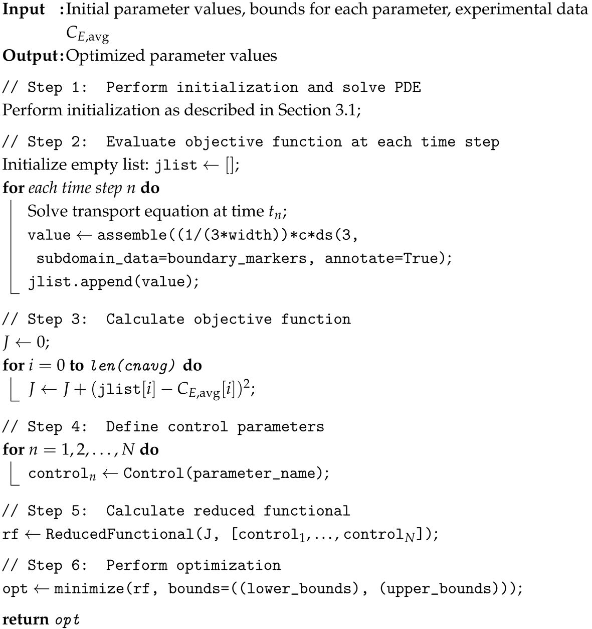
The argument annotate=True signals dolfin to store this information on the tape for later use. The tape recognizes that the objective function is discretized in time and that optimization should be performed over the entire time interval rather than only the final time step.

In addition to the objective function, we use the command Control(variable_name) to identify control variables. Both the objective function and an array of control variables are then passed to the following function:

• rf = ReducedFunctional(J, [control1, ..., controlk])

This function uses dolfin-adjoint’s tape to solve both the PDE and the adjoint equation at each time step required by the minimization method [33].

The second code addition to the implementation described in Section 3.2 is the minimization function call. The minimization function supports multiple optimization methods through its arguments. The standard method used in this research is L-BFGS-B, a limited-memory Broyden–Fletcher–Goldfarb–Shanno (BFGS) implementation with bound constraints on control variables [34]. A brief explanation of this method can be found in [35]. The following command is used to minimize the difference between numerical and experimental data:

• opt = minimize(rf, bounds=((list of lower bounds), (list of upper bounds)))

Methods such as the nonlinear Conjugate Gradient (CG) algorithm, BFGS, and Newton-CG, among others, can be implemented by setting the method parameter in the minimization function call. The choice to use the L-BFGS-B method over others was due to its memory efficiency by approximating the inverse Hessian instead of requiring the computation of the full Hessian like the standard Newton’s method [36]. Additionally, using this bounded method allows us to further constrain our results by providing the option to set reasonable lower and upper bounds on the optimized parameter values. Algorithm 5 presents the details of the minimization implementation.

Algorithm 5: Multi-parameter optimization using dolfin-adjoint

6.2. Optimization Results for Langmuir’s Isotherm

We first investigate the multi-parameter optimization results using Langmuir’s isotherm. Table 11 presents the final optimized parameter values obtained using the method described in Section 6.1, and Figure 12 compares the resulting numerical solution with experimental data.

Table 11. Optimized parameter values for Langmuir’s isotherm when all parameters are allowed to vary. Units are given beside each parameter; (-) indicates the parameter is unitless.

Parameter	Value
$\omega$ (-)	0.9995
${\alpha }_L$ (cm)	0.1261
$\mu$ (-)	0.0284
${\rho }_s$ (mg/mL)	29.86
$k_{eq}$ (mL/mg)	0.7312
$q_{max}$ (mg/mL)	150.1054

Figure 12. Multi-parameteroptimization results for Langmuir’s isotherm using the L-BFGS-B method, a limited-memory Broyden–Fletcher–Goldfarb–Shanno (BFGS) implementation with bound constraints on control variables.

As shown in Figure 12, the numerical results exhibit excellent visual agreement with experimental data. However, the optimal value ${\rho }_s=29.86$ is physically unrealistic for the density of a porous membrane. Additionally, the literature on protein chromatography does not always include ${\rho }_s$ as a parameter (see, for example, [1,6,37]). Once the membrane is submerged in liquid within the chromatography column, its effective density becomes essentially equal to that of the surrounding liquid. Consequently, we fixed ${\rho }_s=1$ and re-optimized the remaining parameters, allowing these parameters to compensate for the constraint.

Table 12 presents the optimal parameter values with ${\rho }_s=1$ fixed, and Figure 13 compares the corresponding numerical solution with experimental data.

Table 12. Optimized parameter values for Langmuir’s isotherm with ${\rho }_s=1$ fixed. Units are given beside each parameter; (-) indicates the parameter is unitless.

Parameter	Value
$\omega$ (-)	0.9869
${\alpha }_L$ (cm)	0.1255
$\mu$ (-)	0.0286
${\rho }_s$ (mg/mL)	1
$k_{eq}$ (mL/mg)	0.6954
$q_{max}$ (mg/mL)	149.9476

Figure 13. Multi-parameter optimization results for Langmuir’s isotherm with ${\rho }_s=1$ fixed, using the L-BFGS-B method.

The unconstrained optimization (Table 11) yields an objective function value of $J=0.7726$, while the constrained optimization with ${\rho }_s=1$ (Table 12) yields $J=0.6041$. Thus, the constrained optimization produces moderately more accurate results while maintaining physical realism.

6.3. Optimization Results for Nfor’s Isotherm

To implement optimization for Nfor’s isotherm, we must define the isotherm such that the minimization package recognizes that $q^n$ and $q^{n-1}$ are updated at each time step. As before, we use the argument annotate=True to signal that this value changes when defining the isotherm expression:

• q_n = Expression(*Nfor’s isotherm definition*, *parameter definitions*,
•           annotate=True)

With this modification, we optimized the parameters $\omega$, ${\alpha }_L$, $\mu$, $k_{eq}$, and $q_{max}$ while fixing ${\rho }_s=1$ and setting all other parameters to their original values from Table 2. The results are presented in Table 13 and Figure 14. Comparison with Figure 3b (original parameter values) demonstrates a substantially improved fit to experimental data.

Table 13. Optimized parameter values for Nfor’s isotherm. Units are given beside each parameter; (-) indicates the parameter is unitless.

Parameter	Value	Parameter	Value
${\omega }^{†}$ (-)	0.9414	v (-)	0.1
${\alpha }_L^{†}$ (cm)	0.0464	r (-)	1
${\mu }^{†}$ (-)	0.3014	z (-)	1
${\rho }_s$ (mg/mL)	1	$c_s$ (M)	0.37
$k_{eq}^{†}$ (mL/mg)	502.4774	$c_m$ (M)	55.5
$q_{max}^{†}$ (mg/mL)	216.0372	$k_s$ (M−1)	$-0.1$
$\mathrm{\Lambda }$ (M)	0.3400	$k_p$ (mL/mg)	$-0.1$

^† Parameter was optimized; all others were fixed at original values from Table 2.

Figure 14. Multi-parameter optimization results for Nfor’s isotherm over parameters $\omega$, ${\alpha }_L$, $\mu$, $k_{eq}$, and $q_{max}$.

We also attempted to optimize all remaining parameters in Nfor’s isotherm while maintaining ${\rho }_s=1$. However, this optimization produced negligible changes from the original parameter values. Subsequently, we fixed $\omega$, ${\alpha }_L$, $\mu$, ${\rho }_s$, $k_{eq}$, and $q_{max}$ to the values in Table 13 and optimized over the remaining parameters (v, r, z, $c_s$, $c_m$, $k_s$, $k_p$, $\mathrm{\Lambda }$). Again, these parameters exhibited insignificant changes. Therefore, our optimal parameter values for Nfor’s isotherm are those presented in Table 13.

7. Sensitivity Analysis

Sensitivity analysis quantifies how perturbations in parameters affect the solution at a particular time. In this section, we derive the sensitivity equations with respect to model parameters and discuss the results for Langmuir’s isotherm. Since we have defined two isotherms, we treat them generally in the sensitivity equations as $q=h(q,C)$. To simplify the partial derivative of h with respect to any parameter $\beta$, we perform the following derivation:

$$\begin{array}{cc}\hfill {\displaystyle \frac{\partial q}{\partial \beta }}& ={\displaystyle \frac{\partial h(q,C)}{\partial \beta }}={\displaystyle \frac{\partial h}{\partial C}}{\displaystyle \frac{\partial C}{\partial \beta }}+{\displaystyle \frac{\partial h}{\partial q}}{\displaystyle \frac{\partial q}{\partial C}}{\displaystyle \frac{\partial C}{\partial \beta }}\hfill \\ \hfill {\displaystyle \frac{\partial q}{\partial \beta }}-{\displaystyle \frac{\partial h(q,C)}{\partial \beta }}& =0\hfill \\ \hfill {\displaystyle \frac{\partial q}{\partial \beta }}-\left({\displaystyle \frac{\partial h}{\partial C}}{\displaystyle \frac{\partial C}{\partial \beta }}+{\displaystyle \frac{\partial h}{\partial q}}{\displaystyle \frac{\partial q}{\partial \beta }}\right)& =0.\hfill \end{array}$$

This simplification yields the recurring coefficient

$${\displaystyle \frac{\partial q}{\partial \beta }}={\displaystyle \frac{\frac{\partial h}{\partial C}}{1-\frac{\partial h}{\partial q}}}{\displaystyle \frac{\partial C}{\partial \beta }},$$

(11)

where $\beta$ represents the parameter under investigation. Table 14 contains the sensitivity equations for each parameter in (1) using Langmuir’s isotherm. For Langmuir’s isotherm, ${\displaystyle \frac{\partial h}{\partial q}}=0$. As in the implementation for Nfor’s isotherm, lagging h in time provides a method to evaluate $q^n=h(q^{n-1},C^{n-1})$.

Table 14. Sensitivity equations for each parameter using Langmuir’s isotherm.

Parameter	Sensitivity Equation
$\omega$	${\displaystyle \frac{\partial C}{\partial t}+\omega \frac{\partial }{\partial t}\frac{\partial C}{\partial \omega }-{\rho }_s\frac{\partial q}{\partial t}+(1-\omega ){\rho }_s\frac{\partial }{\partial t}\frac{\partial q}{\partial \omega }+\nabla ·\left(\mathbf{u}\frac{\partial C}{\partial \omega }\right)-\nabla ·\left(\mathbf{D}\nabla \frac{\partial C}{\partial \omega }\right)=0}$
${\alpha }_L$	${\displaystyle \omega \frac{\partial }{\partial t}\frac{\partial C}{\partial {\alpha }_L}+(1-\omega ){\rho }_s\frac{\partial }{\partial t}\frac{\partial q}{\partial {\alpha }_L}+\nabla ·\left(\mathbf{u}\frac{\partial C}{\partial {\alpha }_L}\right)-\nabla ·\left(\frac{\partial \mathbf{D}}{\partial {\alpha }_L}\nabla C\right)-\nabla ·\left(\mathbf{D}\nabla \frac{\partial C}{\partial {\alpha }_L}\right)=0}$
$\mu$	${\displaystyle \omega \frac{\partial }{\partial t}\frac{\partial C}{\partial \mu }+(1-\omega ){\rho }_s\frac{\partial }{\partial t}\frac{\partial q}{\partial \mu }+\nabla ·\left(\mathbf{u}\frac{\partial C}{\partial \mu }\right)-\nabla ·\left(\frac{\partial \mathbf{D}}{\partial \mu }\nabla C\right)-\nabla ·\left(\mathbf{D}\nabla \frac{\partial C}{\partial \mu }\right)=0}$
$q_{max}$	${\displaystyle \omega \frac{\partial }{\partial t}\frac{\partial C}{\partial q_{max}}+(1-\omega ){\rho }_s\frac{\partial }{\partial t}\frac{\partial q}{\partial q_{max}}+\nabla ·\left(\mathbf{u}\frac{\partial C}{\partial q_{max}}\right)-\nabla ·\left(\mathbf{D}\nabla \frac{\partial C}{\partial q_{max}}\right)=0}$
${\rho }_s$	${\displaystyle \omega \frac{\partial }{\partial t}\frac{\partial C}{\partial {\rho }_s}+(1-\omega )\frac{\partial q}{\partial t}+(1-\omega ){\rho }_s\frac{\partial }{\partial t}\frac{\partial q}{\partial {\rho }_s}+\nabla ·\left(\mathbf{u}\frac{\partial C}{\partial {\rho }_s}\right)-\nabla ·\left(\mathbf{D}\nabla \frac{\partial C}{\partial {\rho }_s}\right)=0}$
$k_{eq}$	${\displaystyle \omega \frac{\partial }{\partial t}\frac{\partial C}{\partial k_{eq}}+(1-\omega ){\rho }_s\frac{\partial }{\partial t}\frac{\partial q}{\partial k_{eq}}+\nabla ·\left(\mathbf{u}\frac{\partial C}{\partial k_{eq}}\right)-\nabla ·\left(\mathbf{D}\nabla \frac{\partial C}{\partial k_{eq}}\right)=0}$

Once the sensitivity equations are obtained, we derive their weak formulations to enable FEniCS to solve them at each time step. Time derivatives in the weak formulation are handled as described in Section 3.2. As an example, the weak form of the sensitivity equation for $q_{max}$ is given by

$$\begin{array}{cc}\hfill & {\int }_{\mathrm{\Omega }}\left(\omega {\displaystyle \frac{\frac{\partial C^n}{\partial q_{max}}+(1-\omega ){\rho }_s\frac{\frac{\partial h}{\partial C^{n-1}}}{1-\frac{\partial h}{\partial q^{n-1}}}\frac{\partial C^n}{\partial q_{max}}}{\Delta t}}\right)vd\mathbf{x}-{\int }_{\mathrm{\Omega }}\mathbf{u}{\displaystyle \frac{\partial C^n}{\partial q_{max}}}·\nabla vd\mathbf{x}\hfill \\ \hfill & +{\int }_{\mathrm{\Omega }}\mathbf{D}\nabla {\displaystyle \frac{\partial C^n}{\partial q_{max}}}·\nabla vd\mathbf{x}+{\int }_{\partial \mathrm{\Omega }}\mathbf{u}{\displaystyle \frac{\partial C^n}{\partial q_{max}}}·\mathbf{n}vds-{\int }_{\partial \mathrm{\Omega }}\mathbf{D}\nabla {\displaystyle \frac{\partial C^n}{\partial q_{max}}}·\mathbf{n}vds\hfill \\ \hfill & ={\int }_{\mathrm{\Omega }}\left(\omega +(1-\omega ){\rho }_s{\displaystyle \frac{\frac{\partial h}{\partial C^{n-1}}}{1-\frac{\partial h}{\partial q^{n-1}}}}\right){\displaystyle \frac{\frac{\partial C^{n-1}}{\partial q_{max}}}{\Delta t}}vd\mathbf{x}\hfill \\ \hfill & +{\int }_{\mathrm{\Omega }}\left((1-\omega ){\rho }_s{\displaystyle \frac{k_{eq}{C}^{n-1}}{1+k_{eq}{C}^{n-1}}}-(1-\omega ){\rho }_s{\displaystyle \frac{k_{eq}{C}^n}{1+k_{eq}{C}^n}}\right){\displaystyle \frac{v}{\Delta t}}d\mathbf{x}.\hfill \end{array}$$

(12)

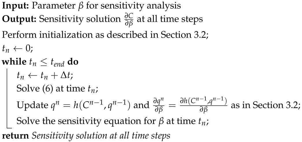
Algorithm 6 shows the implementation steps for solving the sensitivity equations.

Algorithm 6: Solving sensitivity equations for parameter $\beta$

7.1. Sensitivity Analysis with Langmuir’s Isotherm

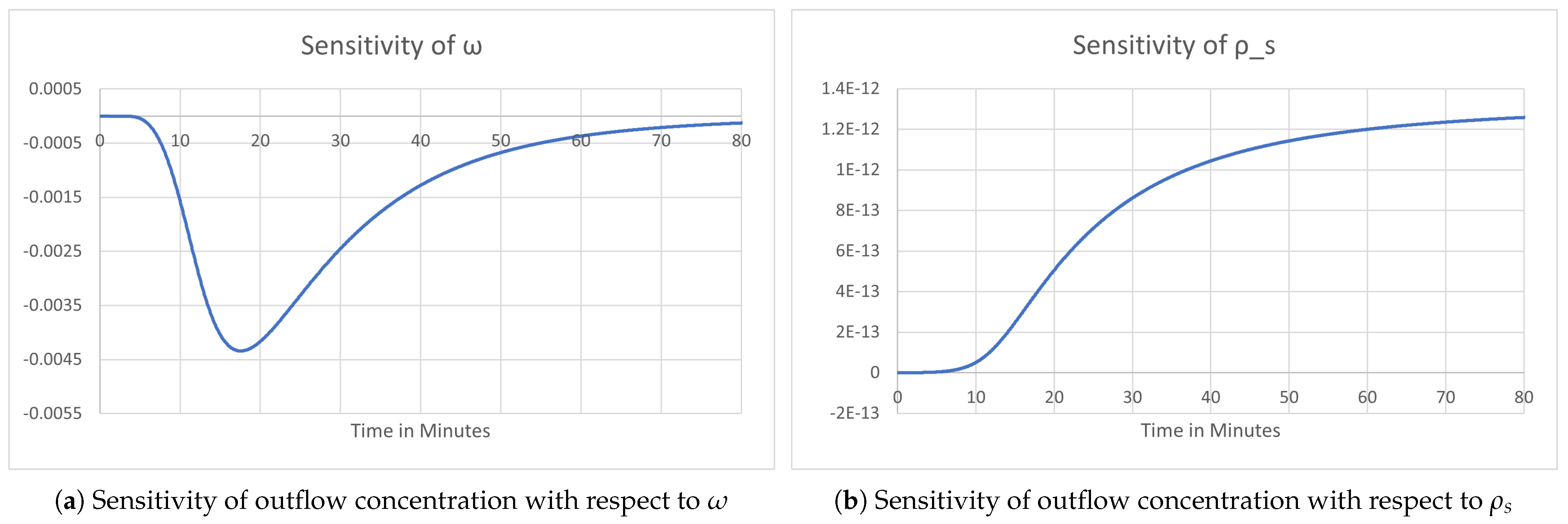
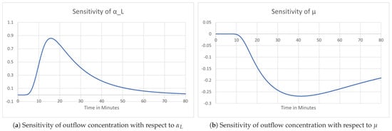
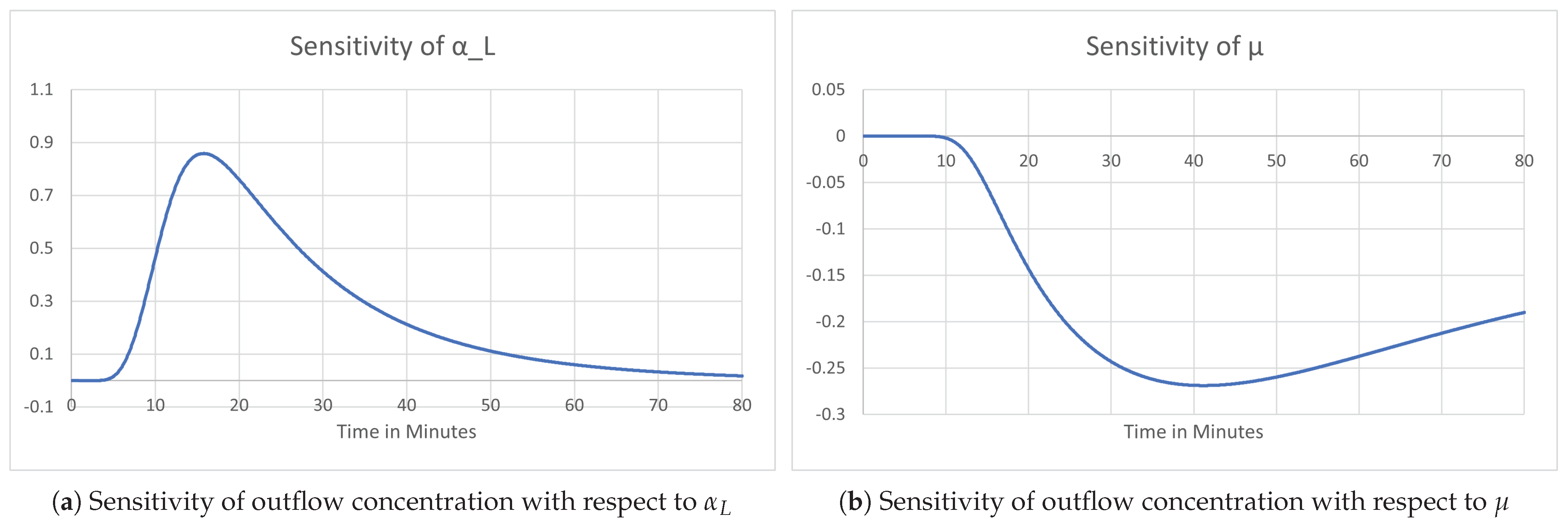
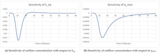
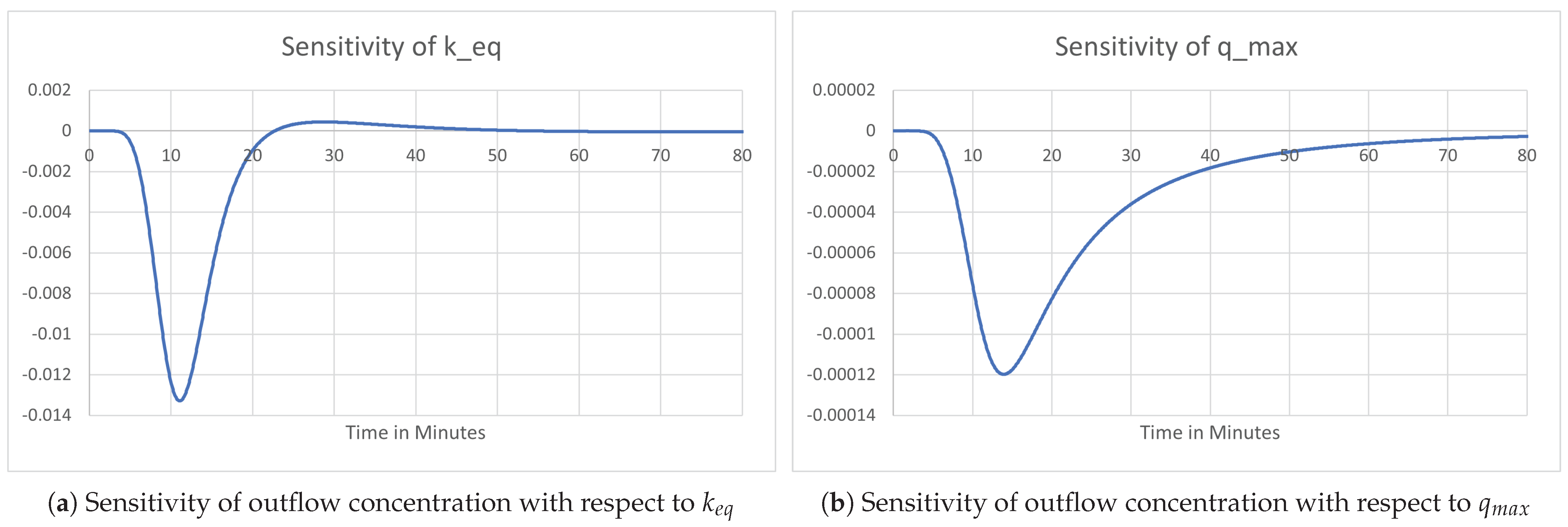
Figure 15, Figure 16 and Figure 17 present the sensitivity analysis results for Langmuir’s isotherm. Using the optimal solution from our multi-parameter optimization, we find that $\omega$, ${\rho }_s$, $k_{eq}$, and $q_{max}$ produce relatively small changes in the outflow concentration, with the largest having magnitude $O\left({10}^{-2}\right)$. In contrast, ${\alpha }_L$ and μ produce larger magnitude changes, indicating that perturbations in the dispersion tensor parameters have a greater effect on outflow concentration than other parameters, which is consistent with [6]. This can be explained by looking at the effects of the parameters on the modeling equations. The dispersion tensor $\mathbf{D}$ appears in the highest-order spatial derivative in the transport equation, so perturbations in ${\alpha }_L$ and μ affect the shape of the entire concentration profile spatially. In contrast, the isotherm parameters ($k_{eq}$, $q_{max}$) appear only in the adsorption term, which shifts the curve temporally but does not reshape the diffusive spread. Comparing the sensitivity solutions in Figure 15, Figure 16 and Figure 17 with the numerical solution in Figure 13, we observe that increases in parameter sensitivity coincide with the rise in outflow concentration in the numerical solutions, generally occurring between $t=10$ and $t=30$ min.

Figure 15. Sensitivity analysis for Langmuir’s isotherm: porosity and density parameters.

Figure 16. Sensitivity analysis for Langmuir’s isotherm: dispersivity parameters.

Figure 17. Sensitivity analysis for Langmuir’s isotherm: adsorption isotherm parameters.

7.2. Sensitivity of the Objective Function

In addition to the sensitivity of the model solution, we can examine the sensitivity of the objective function with respect to each parameter. The sensitivity of the objective function (10) with respect to a general parameter $\beta$ is

$${\displaystyle \frac{\partial J}{\partial \beta }}=2{\int }_0^T\left(C_{(N,avg)}\left(t\right)-C_{(E,avg)}\left(t\right)\right){\displaystyle \frac{\partial C_{(N,avg)}\left(t\right)}{\partial \beta }}dt.$$

(13)

From Figure 15, Figure 16 and Figure 17, we again conclude that ${\alpha }_L$ and μ have the greatest effect on the objective function. Notably, in all optimization results presented previously, ${\alpha }_L$ and μ exhibited the largest changes from their initial values to achieve improved fits. This consistency between the model sensitivity analysis and the objective function sensitivity analysis validates our optimization results.

Additionally, when considering the objective function sensitivity alongside the original numerical results for Langmuir’s isotherm (Figure 3a), we observe that adjusting certain parameters at specific times may be beneficial. Since minimization seeks a direction of decrease (negative gradient), adjusting ${\alpha }_L$ during the early simulation would more effectively reduce the objective function because $C_{(N,avg)}-C_{(E,avg)}<0$, providing a negative sign in the sensitivity. Since ${\displaystyle \frac{\partial C}{\partial {\alpha }_L}}>0$ from the sensitivity analysis, increasing ${\alpha }_L$ yields a negative value for (13), indicating a direction of decrease. Later in the simulation, when the numerical data exceeds the experimental data ($C_{(N,avg)}-C_{(E,avg)}>0$), further increases in ${\alpha }_L$ would be counterproductive. However, adjusting μ becomes more beneficial during this phase, as its sensitivity analysis shows it helps decrease the numerical outflow concentration. This observation suggests potential future work investigating time-dependent dispersivity parameters.

We note that the sensitivity and optimization results alone cannot distinguish definitively between true physical dominance of the dispersion parameters and the absorption of model-form error into these parameters. The latter is a known phenomenon in parameter estimation for transport models: because the dispersion tensor governs the highest-order spatial derivative, it has the greatest mathematical flexibility to compensate for structural modeling assumptions, such as constant velocity, instantaneous adsorption, and simplified geometry. Resolving this ambiguity would require either multiple experimental datasets under varying flow conditions to assess the physical consistency of the optimal dispersivity values, or a formal identifiability analysis; both represent valuable directions for future work.

8. Conclusions

Through an initial parameter value investigation and the implementation of a line search algorithm, we identified optimal parameter values individually for Langmuir’s isotherm. We found that the order of sequential optimization significantly affected the accuracy of the fit to experimental data, motivating the need for simultaneous multi-parameter optimization. Using the FEniCS software with the dolfin-adjoint package, we optimized all model parameters simultaneously to obtain numerical results with substantially improved agreement with experimental data.

For the transport equation modeling fluid flow through porous media, we determined the optimal parameter values shown in Table 15. Through sensitivity analysis, we determined that each parameter produces the most significant changes in the outflow solution during the period of rapid concentration increase. Notably, the dispersivity parameters ${\alpha }_L$ and μ induce the largest sensitivity in the solution, consistent with the substantial changes in these parameters observed during optimization.

Table 15. Optimal parameter values from multi-parameter optimization. Units are given beside each parameter; (-) indicates the parameter is unitless.

Parameter	Langmuir	Nfor	Parameter	Langmuir	Nfor
$\omega$ (-)	0.9869	0.9414	$\mathrm{\Lambda }$ (M)	—	0.34
${\alpha }_L$ (cm)	0.1255	0.0464	v (-)	—	0.1
$\mu$ (-)	0.0286	0.3014	r (-)	—	1
${\rho }_s$ (mg/mL)	1	1	z (-)	—	1
$k_{eq}$ (mL/mg)	0.6954	502.4774	$c_s$ (M)	—	0.37
$q_{max}$ (mg/mL)	149.9476	216.0372	$c_m$ (M)	—	55.5
			$k_s$ (M−1)	—	$-0.1$
			$k_p$ (mL/mg)	—	$-0.1$

Several directions for future work remain. First, the dolfin-adjoint package provides numerous optimization methods beyond L-BFGS-B that were not investigated in this research. Future work could compare these methods to determine whether alternative algorithms yield improved results. Additionally, regularization strategies such as Tikhonov or total varation could be explored to prevent overfitting, and uncertainty quantification could be conducted to determine how inaccuracies in the fitted parameter values could affect the predictions of the model.

Second, alternative objective functions could be explored; for instance, Tarafder et al. [1] considered objective functions that maximize yield, purity, and productivity while minimizing material consumption. Such approaches could optimize not only data fitting but also the overall efficiency of the membrane chromatography process.

Third, we maintained consistent time step $\Delta t$ and mesh size h values throughout this research, though smaller values may improve parameter fitting accuracy. However, computational cost is a significant consideration: the line search algorithms required 30 min to a few hours per optimization (with μ optimization requiring the longest time), meaning the full sequential parameter optimization for the line search algorithm could take several hours to a little over a day to optimize all values. For the line search algorithm, adjusting the stopping criteria, step size, or starting farther or closer to a relative minimum would also have effects on the run time. The multi-parameter optimization required one to two days to successfully run, where the code using Nfor’s isotherm was the longer of the two due to the additional parameters. Decreasing $\Delta t$ and h would substantially increase these computational times; conversely, increasing them would improve run time at the cost of reducing the quality of the results. It is also worth noting that these scripts were run on a laptop that was often in use during part or all of the run times, which can have an effect on computational efficiency. Using a computer with greater processing power or having a dedicated computer to execute the code could potentially decrease the run time. Additionally, updates have been made to the Fenics software since this research was conducted which may produce more computationally efficient results. Nonetheless, investigating the trade-off between accuracy and computational cost remains valuable future work.

Fourth, certain model assumptions could be relaxed to enhance physical realism. We assumed constant parameter values, but time-dependent or concentration-dependent parameters may better capture the physical behavior. For example, porosity $\omega$ may decrease over time as more protein accumulates in the membrane, suggesting a dependence on either time or local concentration. Similarly, the dispersivity parameters could vary with flow conditions. Additionally, prior work [13] shows how varying the velocity profiles greatly affects the outflow concentration results; consequently, incorporating variable velocity could improve the accuracy of the simulation results. Finally, we assumed instantaneous adsorption, which may not accurately represent the system throughout the entire simulation. Future work could investigate non-instantaneous adsorption with a kinetic rate that depends on t, C, q, or some combination thereof.

Last, machine learning methods could be used to augment the mechanistic models employed in this paper. For example for the situation modeled in this paper, a physics-informed neural network (PINN) could be utilized by representing the modeling transport equation as a loss function while the adsorption isotherms are derived from empirical data. Such hybrid data-drive/mechanistic approaches represent an interesting future direction.

This research demonstrates that multi-parameter optimization with gradient-based methods provides an effective framework for calibrating transport models in porous media. The sensitivity analysis confirms that the optimization successfully identified the most influential parameters and adjusted them appropriately to achieve agreement with experimental data. The methods developed here are applicable to other transport phenomena in porous media and provide a foundation for further refinement of membrane chromatography models.

References

- Tarafder, A. Modeling and multi-objective optimization of a chromatographic system. In Multi-Objective Optimization in Chemical Engineering; Bonilla-Petrociolet, A., Rangaiah, G., Eds.; Wiley: Hoboken, NJ, USA, 2013; pp. 369–398. [Google Scholar]
- Bernau, C.R.; Knödler, M.; Emonts, J.; Jäpel, R.C.; Buyel, J.F. The use of predictive models to develop chromatography-based purification processes. Front. Bioeng. Biotechnol. 2022, 10, 1009102. [Google Scholar] [CrossRef] [Scilit] [PubMed]
- Bio-Rad Laboratories. Liquid Chromatography Principles; Bio-Rad Laboratories: Hercules, CA, USA, 2023. [Google Scholar]
- Wilson, A.B. Modeling, Analysis, and Simulation of Adsorption in Functionalized Membranes. Ph.D. Thesis, Clemson University, Clemson, SC, USA, 2016. [Google Scholar]
- Hahn, T.; Sommer, A.; Osberghaus, A.; Heuveline, V.; Hubbuch, J. Adjoint-based estimation and optimization for column liquid chromatography models. Comput. Chem. Eng. 2014, 64, 41–54. [Google Scholar] [CrossRef] [Scilit]
- Lalli, E.; Sarti, G.C.; Boi, C. Use of the Dispersion Coefficient as the Sole Structural Parameter to Model Membrane Chromatography. Membranes 2022, 12, 668. [Google Scholar] [CrossRef] [Scilit] [PubMed]
- Heinonen, J.; Kukkonen, S.; Sainio, T. Evolutionary multi-objective optimization based comparison of multi-column chromatographic separation processes for a ternary separation. J. Chromatogr. A 2014, 1358, 181–191. [Google Scholar] [CrossRef] [Scilit] [PubMed]
- Bhut, B.; Husson, S. Dramatic performance improvement of weak anion-exchange membranes for chromatographic bioseparations. J. Membr. Sci. 2009, 337, 215–233. [Google Scholar] [CrossRef] [Scilit]
- Bhut, B.; Wickramasinghe, S.; Husson, S. Preparation of high-capacity, weak anion-exchange membranes for protein separations using surface-initiated atom transfer radical polymerization. J. Membr. Sci. 2008, 325, 176–183. [Google Scholar] [CrossRef] [Scilit]
- Singh, N.; Wang, J.; Ulbrict, M.; Wickramasinghe, S.; Husson, S. Surface-initiated atom transfer radical polymerization: A new method for the preparation of polymeric membrane adsorbers. J. Membr. Sci. 2008, 309, 64–72. [Google Scholar] [CrossRef] [Scilit]
- Wang, J.; Sproul, R.T.; Anderson, L.S.; Husson, S.M. Development of multimodal membrane adsorbers for antibody purification using atom transfer radical polymerization. Polymer 2014, 55, 1404–1411. [Google Scholar] [CrossRef] [Scilit]
- Wang, J.; Jenkins, E.; Robinson, J.; Wilson, A.; Husson, S. A new multimodal membrane adsorber for monoclonal antibody purifications. J. Membr. Sci. 2015, 492, 137–146. [Google Scholar] [CrossRef] [Scilit]
- Wilson, A.; Wang, J.; Jenkins, E.; Husson, S. Numerical Simulation of Solid Phase Adsorption Models Using Time-Integrated, Up-winded Finite Element Strategies. IEEE Comput. Sci. Eng. 2020, 22, 64–78. [Google Scholar] [CrossRef] [Scilit]
- Wilson, A.; Jenkins, E. Analysis of a fully implicit SUPG scheme for a filtration and separation model. Comput. Appl. Math. 2020, 39, 89. [Google Scholar] [CrossRef] [Scilit]
- Wilson, A.; Jenkins, E. Numerical Simulation of Chemical Separations Using Multimodal Adsorption Isotherms. Res. App. Math. 2020, 7, 100122. [Google Scholar] [CrossRef] [Scilit]
- Wilson, A.; Jenkins, E. Second Order Methods for Nonlinear Adsorption Problems. In 2022 Spring Western Sectional Meeting; American Mathematical Society: Providence, RI, USA, 2025. [Google Scholar]
- Allgor, R.; Barton, P. Mixed-integer dynamic optimization I: Problem formulation. Comput. Chem. Engrg. 1999, 23, 567–584. [Google Scholar] [CrossRef] [Scilit]
- Barton, P.; Lee, C.; Yunt, M. Optimization of hybrid systems. Comput. Chem. Engrg. 2006, 30, 1576–1589. [Google Scholar] [CrossRef] [Scilit]
- van Beijeren, P.; Kreis, P.; Zeiner, T. Development of a generic process model for membrane adsorption. Comput. Chem. Eng. 2013, 53, 86–101. [Google Scholar] [CrossRef] [Scilit]
- de Marsily, G. Quantitative Hydrogeology: Groundwater Hydrology for Engineers; Academic Press: Cambridge, MA, USA, 1986. [Google Scholar]
- Nfor, B.K.; Noverraz, M.; Chilamkurthi, S.; Verhaert, P.D.; van der Wielen, L.A.; Ottens, M. High-throughput isotherm determination and thermodynamic modeling of protein adsorption on mixed mode adsorbents. J. Chromatogr. A 2010, 1217, 6829–6850. [Google Scholar] [CrossRef] [Scilit] [PubMed]
- Langtangen, H.P.; Logg, A. Solving PDEs in Python–The FEniCS Tutorial Volume I; Center for Biomedical Computing, Simula Research Laboratory and Department of Informatics, University of Oslo: Oslo, Norway, 2017. [Google Scholar]
- Bochev, P.; Gunzburger, M. Least-Squares Finite Element Methods; Springer: Berlin/Heidelberg, Germany, 2006; Volume 166. [Google Scholar]
- Kurowski, P.M. Finite Element Analysis for Design Engineers; SAE International: Warrendale, PA, USA, 2022. [Google Scholar]
- Royden, H.L.; Fitzpatrick, P. Real Analysis; Macmillan: New York, NY, USA, 1988; Volume 32, pp. 135–143. [Google Scholar]
- Leoni, G. A First Course in Sobolev Spaces; American Mathematical Society: Providence, RI, USA, 2017; p. 230. [Google Scholar]
- Funke, S.W.; Farrell, P.E. A framework for automated PDE-constrained optimisation. arXiv 2013, arXiv:1302.3894. [Google Scholar]
- Suen, S.Y.; Etzel, M. A Mathematical Analysis of Affinity Membrane Bioseparations. Chem. Eng. Sci. 1992, 47, 1355–1364. [Google Scholar] [CrossRef] [Scilit]
- Agarwal, N.; Semmens, M.; Novak, P.; Hozalski, R. Zone of influence of a gas permeable membrane system for delivery of gases to groundwater. Water Resour. Res. 2005, 41, W05017. [Google Scholar] [CrossRef] [Scilit]
- Xu, M.; Eckstein, Y. Statistical analysis of the relationships between dispersivity and other physical properties of porous media. Hydrogeol. J. 1997, 5, 4–20. [Google Scholar] [CrossRef] [Scilit]
- Kelley, C.T. Iterative Methods for Optimization; SIAM: Philadelphia, PA, USA, 1999. [Google Scholar]
- Dolfin-Adjoint. Documentation for Pyadjoint; Dolfin-Adjoint Development Team: Oslo, Norway, 2023. [Google Scholar]
- Funke, S.W. Optimal Control of the Poisson Equation; Dolfin-Adjoint Development Team: Oslo, Norway, 2023. [Google Scholar]
- Dolfin-Adjoint. PDE-Constrained Optimisation; Dolfin-Adjoint Development Team: Oslo, Norway, 2023. [Google Scholar]
- Lam, A. BFGS in a Nutshell: An Introduction to Quasi-Newton Methods; Towards Data Science: San Francisco, CA, USA, 2022. [Google Scholar]
- Zhang, Z.; Yuan, G.; Qin, Z.; Luo, Q. An improvement by introducing LBFGS idea into the 804 Adam optimizer for machine learning. Expert Syst. Appl. 2026, 296, 129002. [Google Scholar] [CrossRef] [Scilit]
- Dimartino, S.; Boi, C.; Sarti, G.C. A validated model for the simulation of protein purification through affinity membrane chromatography. J. Chromatogr. A 2011, 1218, 1677–1690. [Google Scholar] [CrossRef] [Scilit] [PubMed]
Disclaimer/Publisher’s Note: The statements, opinions and data contained in all publications are solely those of the individual author(s) and contributor(s) and not of MDPI and/or the editor(s). MDPI and/or the editor(s) disclaim responsibility for any injury to people or property resulting from any ideas, methods, instructions or products referred to in the content. |
© 2026 by the authors. Licensee MDPI, Basel, Switzerland. This article is an open access article distributed under the terms and conditions of the Creative Commons Attribution (CC BY) license.