Invariant-Based Analysis of Transient Gas Flow and Optimal Valve Spacing in Pipelines

Abstract

Leakage-induced transients in natural gas transmission pipelines can significantly affect operational safety and emergency response. This study develops a physics-based analytical framework for predicting transient pressure evolution, leakage dynamics, and emergency valve response in high-pressure gas pipelines while deriving a closed-form criterion for optimal valve spacing. The governing equations of compressible gas flow are reduced to a diffusion-type model incorporating acoustic wave propagation and frictional attenuation. A dynamic Robin-type boundary condition is introduced to describe valve–pipeline interactions, and closed-form analytical solutions are obtained using the Laplace transform method. An analytical leakage function and an explicit valve spacing criterion are derived directly from the governing equations and boundary conditions. Parametric investigations under representative transmission pipeline operating conditions demonstrate that the optimal valve spacing depends systematically on attenuation characteristics, activation thresholds, and allowable response times. The analytical solution further predicts a narrow quasi-invariant valve activation interval of approximately 112–116 s, which is theoretically explained through the dominant acoustic–diffusive balance of the proposed model. Verification against an independent finite difference solution shows excellent agreement, with the maximum relative deviation remaining below 1%, thereby confirming the accuracy and numerical consistency of the analytical formulation. The proposed framework provides a physically interpretable and computationally efficient tool for leakage assessment, emergency valve design, and safety-oriented analysis of conventional natural gas transmission pipelines.

1. Introduction

1.1. Background and Motivation

The safe operation of high-pressure gas transmission pipelines depends on the accurate prediction of transient flow behavior under abnormal operating conditions, particularly during leakage events. When a leak occurs, pressure disturbances propagate along the pipeline as coupled acoustic and diffusive waves whose evolution is governed by gas compressibility, hydraulic resistance, and boundary interactions. Understanding these transient processes is essential for leak isolation, emergency response, and pipeline safety assessment [1,2,3,4].

Current engineering practice relies on emergency shut-off valves installed at prescribed intervals along transmission pipelines. International standards, including API RP 14E [5], ISO 13623 [6], and IGEM/TD/1 [7], provide recommendations for valve placement based primarily on operational and safety considerations. Typical valve spacing ranges from 25 to 40 km. However, these recommendations do not explicitly incorporate the transient gas dynamic mechanisms governing pressure propagation and emergency valve response during leakage events.

Recent studies have substantially advanced the understanding of transient gas flow behavior in transmission pipelines through analytical, numerical, and coupled multiphysics approaches. Finite volume and finite element formulations have been widely employed to simulate leakage-induced pressure transients, while optimization-based methodologies have been developed to improve emergency valve placement and pipeline safety. More recently, coupled pipeline system models and transient flow analyses have focused on enhancing leakage detection, pressure wave interpretation, and safety-oriented operational strategies under increasingly complex operating conditions [8,9,10,11]. Despite these advances, relatively few studies have established explicit closed-form analytical relationships linking transient pressure evolution, leakage dynamics, and emergency valve spacing within a unified mathematical framework.

Existing approaches to valve spacing design may be classified as empirical, simulation-based, and optimization-based. Empirical methods are simple to apply but provide only a limited representation of transient flow processes. Numerical simulations accurately reproduce complex transient behavior and remain indispensable for detailed engineering analyses; however, they generally require repeated computations for different operating scenarios and parameter combinations. Optimization techniques improve design flexibility but are likewise dependent on the selected operating conditions and computational framework [9]. Consequently, analytical approaches remain of considerable interest because they provide complementary closed-form relationships that facilitate physical interpretation, rapid parametric assessment, and preliminary engineering design within a unified mathematical framework. The present study is intentionally restricted to conventional natural gas transmission pipelines in order to establish a rigorous analytical framework for transient pressure evolution, leakage dynamics, and emergency valve response. Future work will focus on extending the proposed analytical formulation to multicomponent gas mixtures and non-isothermal transient flow conditions [10,11,12]. These developments motivate the need for physically consistent analytical models suitable for both safety assessment and engineering design.

Numerical methods such as the finite volume method (FVM) and finite element method (FEM) have become indispensable tools for analyzing transient gas flow phenomena in complex pipeline systems because they accurately capture nonlinear flow behavior, complex geometries, and realistic operating conditions. However, these methods generally require repeated numerical computations for each parameter configuration and often provide limited analytical insight into the explicit relationships among governing physical parameters. In contrast, analytical models provide closed-form expressions that reveal the dependence of transient pressure evolution, leakage dynamics, and valve response directly on the governing parameters. Therefore, the present work is intended to complement, rather than replace, established numerical simulation techniques by providing a physically interpretable analytical framework that is also suitable for rapid engineering assessment and preliminary design.

1.2. Research Gap and Contributions

Considerable research has been devoted to transient gas flow modeling, leak detection, and emergency isolation in pipeline systems [13,14,15]. Previous studies have investigated pressure wave propagation, state estimation techniques, and numerical optimization of valve placement. Despite these advances, several limitations remain.

First, emergency valves are frequently represented using simplified static boundary conditions, which do not fully reflect the interaction between transient pressure decay and valve response. Second, leakage behavior is often introduced through empirical assumptions rather than derived directly from governing flow equations. Third, most available approaches rely on numerical simulations or scenario-specific optimization procedures, making it difficult to establish explicit relationships between leakage characteristics and valve placement.

To address these limitations, the present study develops a fully analytical framework for transient leak-induced gas flow and emergency valve response in transmission pipelines. The proposed formulation combines transient flow dynamics, leakage evolution, and valve operation within a unified mathematical model.

The main contributions of the study are:

• The formulation of a dynamic Robin-type boundary condition describing emergency valve response;
• The derivation of an analytical leakage function directly from the governing transient-flow model;
• The establishment of a closed-form analytical expression for optimal emergency valve spacing;
• The identification of a quasi-invariant valve activation time, indicating a stable acoustic–diffusive equilibrium during transient pipeline operation.

These results provide analytical insight into the relationship between leakage development, pressure wave propagation, and emergency isolation while offering practical guidance for the design and operation of gas transmission pipelines.

2. Theoretical Model and Governing Equations

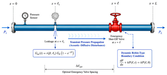
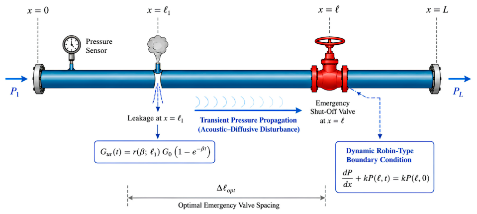
A pressurized transmission pipeline of length L is considered, with a leakage point located at x = ℓ₁ and an emergency shut-off valve located at x = ℓ. The gas flow is assumed to be one-dimensional, isothermal, and compressible (Figure 1). The transported medium is assumed to be conventional natural gas. Accordingly, the acoustic velocity ccc is treated as the characteristic wave propagation parameter determined by the thermophysical properties of the gas under the representative operating conditions considered in this study. Frictional resistance is represented by a linearized Darcy–Weisbach coefficient (2a).

Figure 1. Physical configuration of the pipeline system considered in the analytical model.

A localized leakage at x = ℓ₁ generates a transient pressure disturbance described by the analytically derived leakage function G_ut(t). The emergency shut-off valve located at x = ℓ is represented through a dynamic Robin-type boundary condition. The analytical formulation establishes the relationship between transient pressure attenuation, valve response, and optimal valve spacing Δℓ_opt.

The acoustic velocity c is treated as a characteristic parameter of conventional natural gas and is assumed constant for the representative operating conditions considered in the present analysis. This affects the pressure diffusivity,

$$D={\displaystyle \frac{c^2}{2a}},$$

and therefore modifies the propagation and attenuation of leak-induced pressure disturbances. For conventional natural gas, the acoustic velocity is determined by the thermophysical properties of the gas and constitutes one of the principal parameters governing transient pressure wave propagation and hydraulic attenuation in transmission pipelines [9,10]. In the present formulation, this effect is incorporated through the acoustic velocity c, the attenuation coefficient β, and the valve sensitivity parameter κ.

The following assumptions are adopted: one-dimensional compressible flow, small-disturbance linearization, isothermal conditions, ideal gas behavior P = ρc², and linearized friction. The isothermal approximation is appropriate for long buried transmission pipelines, where the surrounding soil damps short-term temperature variations caused by leakage expansion [16]. Accordingly, temperature effects are incorporated indirectly through the representative thermophysical properties adopted in the analytical model, whereas localized thermal variations are assumed to have a negligible influence on the large-scale transient pressure propagation considered in the present study. Temperature-induced changes in density and sound velocity are therefore treated as secondary effects compared with the dominant pressure diffusion dynamics [3,4]. Transient gas flow is governed by the one-dimensional continuity and momentum equations [17,18]:

$${\displaystyle \frac{\partial \rho }{\partial t}}+{\displaystyle \frac{\partial \rho v}{\partial x}}=0,$$

$${\displaystyle \frac{\partial v}{\partial t}}+{\displaystyle \frac{1}{\rho }}{\displaystyle \frac{\partial P}{\partial x}}+2av=0$$

where ρ is the gas density, v is the velocity, G = ρv is the mass flow variable, and P is the pressure. Using P = ρc² and eliminating the velocity term, the governing equation reduces to the pressure diffusion form

$${\displaystyle \frac{\partial P\left(x,t\right)}{\partial t}}=D{\displaystyle \frac{{\partial }^{2}P\left(x,t\right)}{\partial x^2}}$$

(1)

where $D={\displaystyle \frac{c^2}{2a}}$ is the effective pressure diffusivity.

The detailed derivation of Equation (1) from the linearized continuity and momentum equations, together with the diffusion approximation adopted in the present study, is provided in Appendix A.

The initial pressure distribution before leakage is assumed to be linear:

$$P\left(x,0\right) =P_1-2a{G}_{0}x$$

(2)

where P₁ is the inlet pressure and G₀ is the initial mass flow rate at x = 0.

The boundary and interface conditions are defined as follows. At the inlet, a constant supply condition is imposed:

$$G\left(0,t\right)=G_0\Rightarrow {\left.{\displaystyle \frac{\partial P}{\partial x}}\right|}_{x=0}=-2a{G}_0$$

(3)

At the leakage point, pressure continuity and mass flow discontinuity are imposed:

$$\begin{array}{l}{P}_1\left({\mathcal{l}}_1,t\right)=P_2\left({\mathcal{l}}_1,t\right),\\ {\left.{\displaystyle \frac{\partial P_2}{\partial x}}\right|}_{x={\mathcal{l}}_1}-{\left.{\displaystyle \frac{\partial P_1}{\partial x}}\right|}_{x={\mathcal{l}}_1}=-2a{G}_{ut}\left(t\right)\end{array}$$

(4)

where G_ut(t) is the transient leakage discharge.

At the valve location x = ℓ, a dynamic Robin-type boundary condition is introduced:

$${\left.{\displaystyle \frac{\partial P}{\partial x}}\right|}_{x=\mathcal{l}}+\kappa P\left(\mathcal{l},t\right)=\kappa P\left(\mathcal{l},0\right)$$

(5)

The parameter κ represents the effective pressure feedback gain of the valve controller.

It does not correspond to a single measurable mechanical quantity such as actuator stiffness, valve travel, or closure time. Instead, it is an equivalent boundary parameter characterizing the overall hydraulic response of the valve–controller assembly.

The limiting cases κ = 0 and κ → ∞ correspond to Neumann-type and Dirichlet-type behavior, respectively. Thus, the boundary condition links pressure decay at the valve location with the valve response during leakage-induced transients.

The Robin boundary condition represents a linearized dynamic interaction between the transient pressure field and the emergency shut-off valve. The parameter κ characterizes the effective sensitivity of the valve controller to pressure deviations and determines the coupling strength between the hydraulic response of the pipeline and the valve actuation mechanism. Small values of κ correspond to weak pressure feedback and delayed valve response, whereas larger values represent stronger feedback and faster valve activation.

Accordingly, Equation (5) should be interpreted as an effective linear boundary model describing the hydraulic influence of the emergency valve rather than a detailed mechanistic model of valve closure dynamics.

The associated fundamental decay rate ω₁ lies between the Neumann and Dirichlet limits for Robin-type boundary conditions. For typical high-pressure gas transmission pipelines, reported values of ω₁ are approximately 0.15–0.25 s⁻¹, which is consistent with the representative value ω₁ = 0.2 s⁻¹ used in this study [3,5].

For the representative transmission pipeline conditions investigated, the corresponding dimensionless valve sensitivity parameter is of the order

$$\kappa =O({10}^{-3}),$$

which is consistent with practical emergency shut-off valves operating under proportional pressure feedback control. The adopted parameter range therefore represents realistic engineering conditions rather than an arbitrary numerical choice.

The leakage discharge is represented by the analytically derived function

$$G_{ut}\left(t\right)=r\left(\beta ;{\mathcal{l}}_1\right)G_0\left(1-e^{-\beta t}\right)$$

(6)

where r(β;ℓ₁) is a dimensionless calibration function, β is the leak attenuation coefficient, and t is time after leakage initiation. The calibration function is defined as

$$r \left(\beta ; {\mathcal{l}}_1\right)=1+\alpha \left(1-{\displaystyle \frac{{\mathcal{l}}_1}{L}}\right)exp\left(-{\displaystyle \frac{\beta }{{\beta }_0}}\right),$$

where β is a leak attenuation coefficient dependent on the leak location and pipeline parameters. The physical interpretation and engineering parametrization of the amplification factor r(β;ℓ₁) are discussed in Appendix B. This factor accounts for the combined influence of leak location and hydraulic attenuation on the effective leakage intensity. Consequently, the leakage discharge evolves smoothly from the undisturbed state toward a finite asymptotic value while maintaining a direct connection between leakage dynamics and measurable transient pressure decay.

The present formulation adopts an isothermal approximation for the transient gas flow. This assumption is appropriate for large-scale transmission pipelines because the governing pressure transients propagate over distances that are several orders of magnitude larger than the localized leakage orifice. Although the Joule–Thomson effect may produce a local temperature reduction in the immediate vicinity of the leak, its spatial extent is typically limited to a small region surrounding the leakage opening and has only a minor influence on the large-scale pressure wave propagation considered here. Consequently, the governing equations describe the transient hydraulic response of the pipeline rather than the detailed thermodynamic expansion inside the leakage jet. The proposed analytical formulation is therefore applicable to transmission pipeline operating conditions for which thermal relaxation with the surrounding environment maintains approximately isothermal flow during the transient process.

For high-pressure buried transmission pipelines, the characteristic thermal equilibration length is typically much smaller than the overall pipeline length, while the investigated transient interval (0–300 s) is sufficiently long for radial heat exchange with the pipe wall to reduce local thermal gradients. Accordingly, the isothermal approximation provides a reasonable first-order description of the global transient pressure response.

3. Analytical Solution and Valve Spacing Formulation

3.1. Analytical Solution of the Transient Pressure Field

To obtain an analytical description of leak-induced transient pressure evolution, the Laplace transform is applied to the governing pressure diffusion equation (Equation (1)) [1,11]:

$$s\overline{P}(x,s)-P\left(x,0\right)=D{\displaystyle \frac{d^2\overline{P}}{\partial x^2}}-2a\overline{P}\left(x,s\right)$$

(7)

where $\overline{P}(x,s)$ denotes the Laplace transform of the pressure field and s is the transform variable. The transformed equation admits the general solution

$$\overline{P}\left(x,s\right)=A\mathrm{c}h\left(\lambda x\right)+B\mathrm{s}h\left(\lambda x\right)+{\overline{P}}_{\mathrm{part}}^{\left(p\right)}\left(\mathrm{x},\mathrm{s}\right)$$

(8)

Following inversion of the Laplace-domain solution and application of the interface and boundary conditions, the transient pressure field is represented through modal expansions in the upstream and downstream regions.

• Region I: (0 < x ≤ ℓ₁)

$$P_1\left(x,t\right)=h(x)+{\displaystyle \sum _{n=1}^{\infty }{B}_n\left(t\right)}{\varphi }_n\left(x\right)$$

(9)

• Region II (ℓ₁ < x ≤ ℓ)

$$P_2\left(x,t\right)=h(x)+{\displaystyle \sum _{n=1}^{\infty }{C}_n\left(t\right)}{\varphi }_n(x)$$

(10)

where h(x) denotes the stationary pressure profile, while ${\varphi }_n(x)$ are the eigenfunctions of the Robin Sturm–Liouville problem associated with the global pipeline domain. Their explicit forms, eigenvalue relations, normalization constants, and modal coefficients are derived in Appendix A.6.

3.2. Analytical Leakage Function and Valve Response

A central objective of the present formulation is to derive the leakage discharge directly from the governing equations rather than prescribing it empirically. By combining the flux discontinuity condition at the leak location with the dynamic valve boundary condition, the following Laplace-domain relation is obtained:

$${\overline{G}}_{ut}\left(s\right)=\Lambda \left(\mathcal{l},{\mathcal{l}}_1,\kappa ;s\right)\left[{\displaystyle \frac{P\left(\mathcal{l},0\right)}{s}}-\overline{P}\left(\mathcal{l},s\right)\right]$$

(11)

where Λ(ℓ,ℓ₁,κ;s) is the leak–valve interaction kernel.

Physically, the kernel Λ(ℓ,ℓ₁,κ;s) represents the transfer of leak-induced pressure disturbances from the leak location to the valve through the coupled pipeline–valve system. The Laplace-domain leakage relation in Equation (11) follows from the compatibility conditions of the transformed two-region boundary value problem. The interaction kernel contains the spectral information associated with the inlet condition, the leak interface conditions, and the Robin-type valve boundary condition, as derived in Appendix A.5.

The detailed derivation of the leakage law, including the dominant pole reduction of the leak–valve interaction kernel and the resulting transient leakage function, is presented in Appendix A.5. The resulting analytical leakage law is

$$G_{ut}\left(t\right)=r\left(\beta ;{\mathcal{l}}_1\right)G_0\left(1-e^{-\beta t}\right)$$

(12)

which is subsequently employed in the derivation of the valve pressure response and activation criterion. The analytical leakage law given by Equation (12) is not intended to represent the instantaneous thermodynamic discharge through a suddenly opened leak or rupture. Instead, it describes the effective transient leakage forcing governing the evolution of the large-scale pipeline pressure field after leakage initiation.

Consequently, the condition G_ut(0) = 0 should be interpreted as the reference instant immediately following leakage initiation, when the global pressure disturbance has not yet fully developed along the pipeline. The subsequent exponential evolution reflects the establishment of the large-scale hydraulic response rather than the local compressible discharge inside the leakage opening.

Unlike conventional leak discharge equations, which explicitly depend on the discharge coefficient, leak area, upstream and downstream pressures, and compressible flow regime, the present analytical formulation adopts an effective macroscopic description. The influence of these local physical mechanisms is represented collectively through the measurable attenuation coefficient β, together with the calibration factor r(β,ℓ₁).

The attenuation coefficient β characterizes the decay of the transient pressure field and may be estimated from inlet pressure measurements using

$$P\left(0,t\right)=P_1{e}^{-\beta t}$$

(13)

where P₁ denotes the pre-leak inlet pressure.

A key feature of the proposed analytical framework is that the leakage dynamics are parameterized through the measurable attenuation coefficient β, which can be directly identified from transient inlet pressure measurements using Equation (13). Accordingly, β should not be interpreted as an intrinsic property of the leak itself, but rather as an effective macroscopic transient parameter characterizing the global pressure attenuation in the pipeline.

Consequently, the value of β implicitly reflects the combined influence of several physical factors, including leakage location, leak size and geometry, operating pressure, hydraulic resistance, pipeline configuration (buried or aboveground), and other mechanisms affecting transient pressure propagation. Thus, these physical effects are not neglected but incorporated collectively through a single experimentally identifiable parameter governing the global transient response.

Conventional compressible leak discharge models generally express the leakage rate as a function of the local thermodynamic conditions at the leakage opening, for example,

$$G=C_{d}A\sqrt{2\rho \Delta P}$$

or its compressible flow counterparts.

In contrast, Equation (12) does not seek to model the detailed nozzle flow physics at the leakage orifice. Instead, it represents the effective hydraulic forcing responsible for the global transient pressure evolution governing emergency valve activation. Accordingly, the proposed formulation should be interpreted as a pipeline-scale transient flow model rather than a local leak discharge model.

Consequently, the leakage discharge becomes linked to a measurable transient flow parameter, allowing the analytical model to be calibrated using observed pressure data. To determine the transient pressure response at the valve location, the inlet condition, leak interface conditions, and Robin valve boundary condition are enforced simultaneously. The resulting Laplace-domain solution is

$$\overline{P}\left(\mathcal{l},s\right)={\displaystyle \frac{P\left(\mathcal{l},0\right)}{s}}-{\displaystyle \frac{A\left(\mathcal{l}\right)}{s^2}}-{\displaystyle \frac{B\left(\mathcal{l},\beta \right)}{s+\beta }}$$

(14)

and the corresponding time-domain pressure response becomes

$$P\left(\mathcal{l},t\right)=P\left(\mathcal{l},0\right)-A\left(\mathcal{l}\right)t-B\left(\mathcal{l},\beta \right)e^{-\beta t}$$

(15)

The coefficients A(ℓ) and B(ℓ,β) represent the steady-state and transient components of the valve pressure response, respectively. Their analytical forms are obtained from the transformed boundary value problem by enforcing the inlet, leak interface, and valve boundary conditions. Details of the derivation are provided in Appendix A, particularly Equations (A12)–(A15). Valve activation is assumed to occur when the normalized pressure ratio reaches a prescribed threshold:

$${\displaystyle \frac{P\left(\mathcal{l},t^{\ast }\right)}{P\left(\mathcal{l},0\right)}}={\theta }_{cr}=1-{\displaystyle \frac{A\left(\mathcal{l}\right)}{P\left(\mathcal{l},0\right)}}t-{\displaystyle \frac{B\left(\mathcal{l},\beta \right)}{P\left(\mathcal{l},0\right)}}\left(1-e^{-\beta t^{\ast }}\right)$$

(16)

This condition defines the instant at which the pressure-sensing mechanism initiates automatic valve closure. Equations (15) and (16) represent the general valve pressure response obtained from the transformed boundary value problem. This expression retains the steady component $A(\mathcal{l})$ and the leakage-induced transient component $B(\mathcal{l},\beta )e^{-\beta t}$. In contrast, the dominant-mode expression used later in Appendix A.7 is a reduced design-level approximation obtained by retaining only the leading spatial mode and combining the local leakage attenuation with the global acoustic–diffusive decay rate.

3.3. Optimal Valve Spacing and Parametric Analysis

The analytical solution developed above permits formulation of the emergency valve placement problem as a safety-constrained optimization task. The objective is to maximize the spacing between neighboring emergency shut-off valves while ensuring that transient pressure decay triggers valve activation within the allowable response time.

The optimization problem is expressed as

$$\Delta {\mathcal{l}}_{opt}=\underset{\Delta \mathcal{l}}{max}\{\Delta \mathcal{l}\}, \mathrm{subject} \mathrm{to} {\displaystyle \frac{P(\mathcal{l},t_v)}{P(\mathcal{l},0)}} \le \theta cr, t_v\le t_{max}$$

Substituting the analytical valve pressure solution into the above constraints yields the closed-form expression for the optimal valve spacing:

$$\Delta {\mathcal{l}}_{opt}={\displaystyle \frac{L}{\pi }}\arccos \left[{\theta }_{cr}\exp \left(\left(\beta +{\displaystyle \frac{{\pi }^2{c}^2}{2a{L}^2}}\right)t_{\max }\right)\right]$$

(17)

Equation (17) represents the dominant-mode analytical design criterion and is applicable provided that

$${\theta }_{cr}exp[(\beta +K)t_{max}]\le 1$$

This inequality constitutes the feasibility condition of the dominant-mode approximation. For the representative pipeline investigated in the present study, the valve activation times reported below are evaluated from the complete modal pressure solution (Equations (15) and (16)), whereas Equation (17) provides the corresponding analytical design criterion for preliminary valve spacing assessment.

In the equation, L is the pipeline length, c is the acoustic velocity, β is the attenuation coefficient, t_max is the allowable response time, and θ_cr is the critical pressure ratio defining valve activation. The detailed derivation of Equation (17), including the dominant-mode approximation and valve activation criterion, is provided in Appendix A.7.

The proposed analytical spacing criterion is intended to complement, rather than replace, existing engineering codes and regulatory requirements. Accordingly, the calculated value of Δℓ_opt should be interpreted as an analytical design recommendation to be applied together with the applicable pipeline safety regulations. Furthermore, the parameter t_max represents the allowable pressure threshold activation time of the emergency valve and should not be interpreted as the total mechanical valve closure time.

The resulting relation provides a direct analytical estimate of valve spacing without iterative numerical optimization. Equation (17) enables direct assessment of the combined influence of attenuation, activation threshold, and allowable response time on optimal valve spacing under representative transmission pipeline conditions.

L = 100 km, a = 0.05 s⁻¹, c = 400 m/s.

Three attenuation scenarios were considered:

• ℓ₁ = 12 km → β = 6.4 × 10⁻⁵ s⁻¹ (upstream region);
• ℓ₁ = 48 km → β = 2.1 × 10⁻⁵ s⁻¹ (mid-section);
• ℓ₁ = 84 km → β = 7.4 × 10⁻⁶ s⁻¹ (downstream region).

The investigated parameter domain covers activation thresholds 0.50 ≤ θ_cr ≤ 0.90 and allowable response times 60 s ≤ t_max ≤ 600 s, encompassing the range typically encountered in transmission pipeline safety analyses.

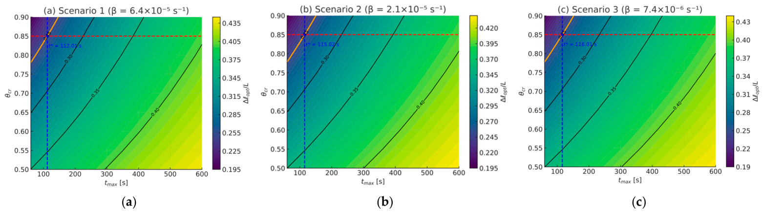
In Figure 2, for the representative design configuration (θ_cr = 0.85 and Δℓ = 25 km), the corresponding valve activation times are obtained from the complete modal analytical solution (Equations (15) and (16)) and are approximately 115 s, 115 s, and 116 s for the three attenuation scenarios considered. Although the attenuation coefficient varies significantly with leak location, the activation time remains within a narrow interval. This behavior arises from the balance between local leak attenuation and global diffusive damping within the pipeline. For the representative system parameters considered here, the characteristic acoustic–diffusive constant remains comparable to the attenuation coefficient β. Consequently, variations in leak position produce only minor changes in the activation time, resulting in a quasi-invariant response:

t^∗ ≈ 112–116 s.

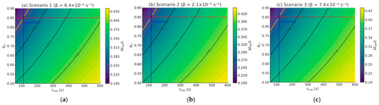
Figure 2. Contour distributions of the normalized optimal valve spacing (Δℓ_opt/L) as functions of the critical pressure ratio (θ_cr) and allowable response time (t_max) for three representative attenuation coefficients.

This result indicates that emergency valve activation is governed primarily by the global transient dynamics of the pipeline system rather than by the leak location alone. The existence of this quasi-invariant activation interval provides a physically interpretable basis for valve spacing design and emergency response planning in long-distance gas transmission pipelines.

4. Results and Discussion

4.1. Boundary Verification and Transient Pressure Response

Representative parameters of a high-pressure gas transmission pipeline were adopted to investigate the transient response characteristics predicted by the analytical model.

P₁ = 5.5 × 10⁵ Pa, G₀ = 30 Pa × s/m, a = 0.05 s⁻¹, c = 400 m/s and L = 100 km.

The dynamic Robin-type valve boundary condition introduced in Equation (5) was implemented to examine representative valve response regimes. The analytical solution satisfies pressure continuity at the leakage location while preserving consistency with both the inlet flow condition and the dynamic Robin-type valve boundary condition. To investigate the influence of leakage position, three representative leakage scenarios were considered,

ℓ₁ = 12 km, ℓ₁ = 48 km, and ℓ₁ = 84 km,

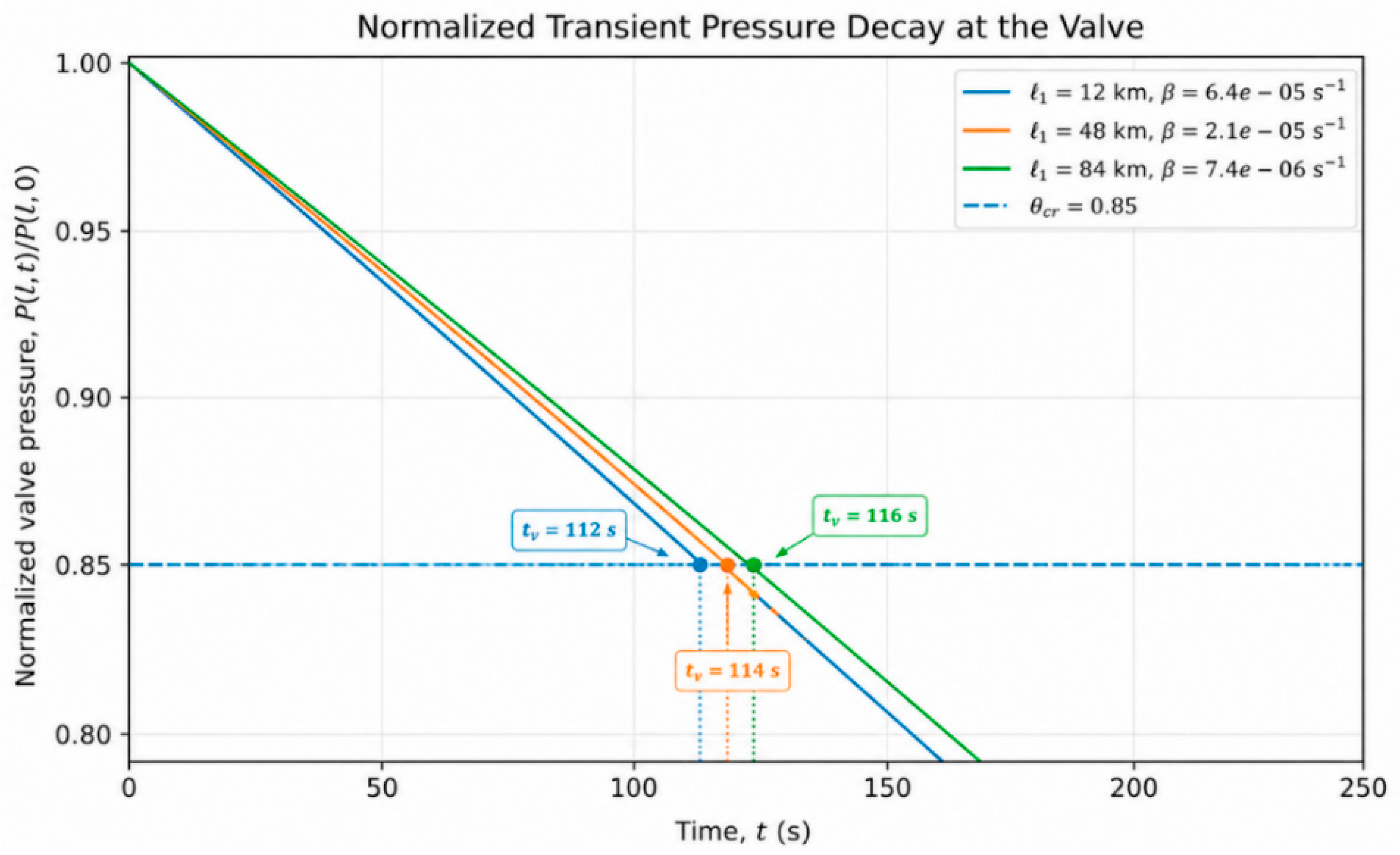
corresponding to upstream, mid-section, and downstream regions of the pipeline, respectively. For each scenario, the normalized valve pressure response P(ℓ,t)/P(ℓ,0) was evaluated using the analytical solution. For the representative threshold θ_cr = 0.85, the analytical model directly yields the corresponding valve activation times.

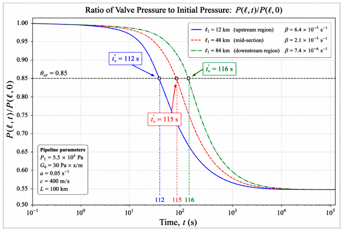
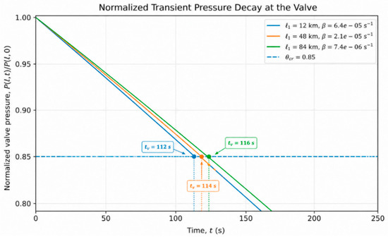
Figure 3 presents the resulting transient pressure decay curves. Although the attenuation coefficient varies from 6.4 × 10⁻⁵ for the upstream leakage scenario to 7.4 × 10⁻⁶ for the downstream case, the corresponding valve activation times remain confined to a narrow interval of approximately 112–116 s.

Figure 3. Normalized transient pressure decay at the valve location for three representative leakage scenarios: upstream (ℓ₁ = 12 km), mid-section (ℓ₁ = 48 km), and downstream (ℓ₁ = 84 km).

The horizontal dashed line denotes the valve activation threshold θ_cr = 0.85, while the vertical dotted lines indicate the corresponding activation times.

The results indicate that the transient valve pressure response exhibits only weak sensitivity to leakage location. Despite substantial variation in the attenuation coefficient, the predicted activation times differ by less than 1%. This behavior suggests the existence of a quasi-invariant response time governed primarily by the global acoustic–diffusive dynamics of the pipeline system rather than by local leakage characteristics alone. From an engineering perspective, this finding is important because it implies that emergency valve actuation may be designed using a nearly location-independent response criterion. Consequently, the proposed analytical framework provides a physically consistent basis for determining optimal valve spacing and for developing robust emergency response strategies in long-distance gas transmission pipelines.

4.2. Optimal Valve Spacing Analysis

Equation (17) provides a direct analytical relationship between optimal valve spacing, activation threshold, and allowable response time, enabling quantitative assessment of emergency valve placement under different operating conditions.

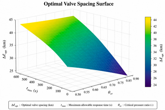
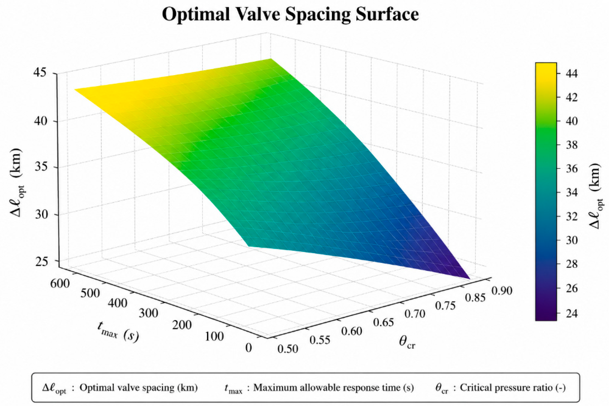
Figure 4 illustrates the resulting optimal valve spacing surface predicted by the analytical formulation.

Figure 4. Optimal emergency valve spacing as a function of the activation threshold and allowable response time.

The results demonstrate that the allowable valve spacing increases with the maximum permissible isolation time. This behavior is expected because longer response times permit transient pressure disturbances to propagate over larger distances before valve activation is required.

The analysis also shows that increasing valve sensitivity (lower activation threshold) reduces the permissible spacing. More sensitive valves respond earlier to pressure decay and therefore require denser installation along the pipeline.

The calculated spacing values generally fall within the range commonly adopted in transmission pipeline practice, indicating consistency between the analytical predictions and engineering experience.

Most importantly, Equation (17) provides a direct analytical relationship between transient flow characteristics and valve placement, eliminating the need for repeated numerical optimization during preliminary design studies.

4.2.1. Representative Engineering Design

The practical applicability of the proposed analytical criterion can be illustrated using the representative transmission pipeline parameters adopted throughout this study. The calculations were performed for a pipeline length of L = 100 km, an acoustic velocity of c = 400 ms⁻¹, a hydraulic resistance coefficient of 2a = 0.1 s⁻¹, a critical valve activation threshold of θ_cr = 0.85, an attenuation coefficient of β = 2.1 × 10⁻⁵ s⁻¹, and an allowable activation time of t_max = 114 s. Substituting these representative values into Equation (17) yields an optimal emergency valve spacing of

$$\Delta {\mathcal{l}}_{opt}=24.9\approx 25 \mathrm{km}$$

where the reported value is obtained directly from the analytical expression without numerical fitting or empirical correction.

This result demonstrates how the proposed analytical formulation can be used directly during the preliminary design stage of transmission pipelines. Unlike empirical spacing recommendations, the present criterion explicitly relates valve placement to measurable transient flow characteristics, attenuation properties, valve response parameters, and the allowable emergency response time. Consequently, the analytical framework provides engineers with a physically interpretable and computationally efficient tool for determining valve locations before performing detailed numerical simulations or final engineering design.

4.2.2. Practical Engineering Perspective

Distributed optical fiber sensing (DOFS) has become an effective technology for real-time leakage monitoring because it provides continuous distributed measurements along the pipeline. However, DOFS primarily serves as a sensing and detection system, whereas the present work addresses a different engineering problem. The proposed analytical framework provides explicit closed-form relationships linking transient pressure evolution, leakage dynamics, valve response characteristics, and optimal emergency valve spacing. Consequently, the analytical model is intended to complement rather than replace distributed sensing technologies. In practical applications, measured pressure or leak detection information obtained from DOFS, SCADA, or other monitoring systems may be directly incorporated into the proposed analytical formulation to support rapid engineering assessment, emergency response planning, and preliminary valve placement design.

4.3. Influence of Leak Attenuation and System Invariance

The influence of leak severity was investigated through the attenuation coefficient β. The selected attenuation coefficients cover the complete range of leak locations considered in this study, representing upstream, mid-section, and downstream leakage scenarios.

• β = 6.4 × 10⁻⁵ s⁻¹;
• β = 2.1 × 10⁻⁵ s⁻¹;
• β = 7.4 × 10⁻⁶ s⁻¹.

The above values correspond to upstream, mid-section, and downstream leakage scenarios, respectively.

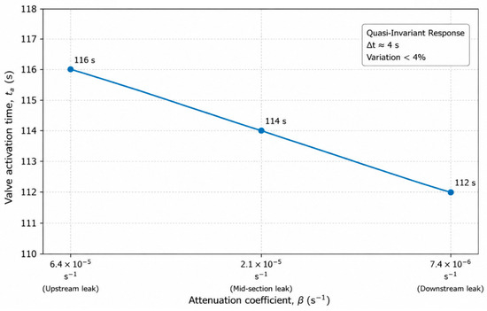
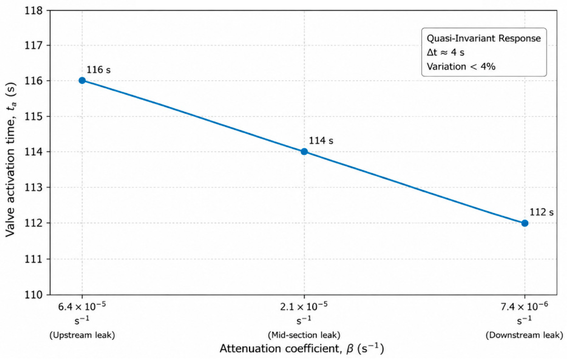
Although Figure 4 demonstrates the effect of attenuation on the optimal valve spacing, it does not directly reveal the corresponding valve activation times. To further investigate the transient response characteristics of the system, the activation times associated with the three representative leakage scenarios were extracted from the analytical pressure response model. Figure 5 demonstrates the corresponding valve activation times associated with the three attenuation regimes.

Figure 5. Quasi-invariant valve activation time under different leak-attenuation conditions.

Figure 5 demonstrates that the valve activation time remains confined to a narrow interval despite substantial variation in the attenuation coefficient. The activation times remain confined to a narrow interval of approximately 112–116 s despite nearly one order of magnitude variation in the attenuation coefficient. This observation is consistent with the quasi-invariant response behavior identified from the transient pressure decay curves in Figure 3. The observed stability of the activation time supports the existence of a characteristic acoustic–diffusive response scale that governs the global transient dynamics of the pipeline system and explains the weak sensitivity of valve activation to leak location and attenuation intensity.

Physical Interpretation of the Quasi-Invariant Activation Interval

The relatively narrow valve activation interval observed in the present study can be explained directly from the analytical activation criterion (Equation (17)). According to the closed-form solution,

$$t_v=-{\displaystyle \frac{1}{\beta +K}}l\ln \left({\displaystyle \frac{{\theta }_{cr}}{\Phi (\Delta \mathcal{l})}}\right),$$

the activation time is governed by two principal factors: the combined attenuation parameter (β + K) and the logarithmic spatial factor associated with the dominant transient mode. Under the representative transmission pipeline conditions investigated,

β = 2.5 × 10⁻⁵–2.5 × 10⁻⁴ s⁻¹,

whereas the valve response coefficient is of order $K\approx {10}^{-2}{ \mathrm{s}}^{-1}$, yielding

$${\displaystyle \frac{\beta }{K}}=O({10}^{-3}{-10}^{-2}).$$

so that $\beta \ll K.$ Consequently,

$${\displaystyle \frac{1}{\beta +K}}\approx {\displaystyle \frac{1}{K}}\left(1-{\displaystyle \frac{\beta }{K}}\right)$$

indicating that moderate variations in the attenuation coefficient introduce only second-order corrections to the activation time. Furthermore, the logarithmic spatial factor varies only weakly over the investigated leak locations. The combined effect of these two characteristics confines the predicted activation time to a narrow interval of approximately 112–116 s throughout the representative parameter range considered.

Accordingly, the observed quasi-invariant activation interval should not be interpreted as a universal characteristic of all gas transmission pipelines. Rather, it represents an asymptotic consequence of the present analytical formulation under the representative operating conditions investigated, reflecting the dominant acoustic–diffusive balance between hydraulic attenuation and valve dynamics. This analytical interpretation is fully consistent with the numerical observations presented in Figure 5 and provides the theoretical explanation for the narrow activation interval reported in the present study.

4.4. Validation Against Benchmark Studies

The physical consistency of the proposed formulation can be assessed through comparison with established analytical and numerical studies of transient gas flow behavior [2,3,4]. Previous studies have shown that leak-induced pressure disturbances propagate as damped diffusion-type waves characterized by exponential pressure decay and finite response times. The present analytical model reproduces these fundamental features.

In particular, the predicted pressure ratio

P(ℓ,t)/P(ℓ,0)

exhibits monotonic exponential-type decay, consistent with diffusion-dominated transient flow behavior. Furthermore, the predicted valve activation interval

t^∗ ≈ 112–116 s

falls within the response time range commonly reported for high-pressure transmission pipelines of comparable length and acoustic velocity.

Benchmark comparisons indicate agreement with established transient flow studies, while independent finite difference verification performed in Section 4.5 yields a maximum deviation below 1%. Although comprehensive experimental datasets for controlled leakage transients in long-distance pipelines remain limited, the observed agreement with established transient flow theory supports the physical plausibility of the proposed analytical formulation and the validity of the dynamic Robin-type boundary condition.

4.5. Numerical Verification Framework

To support the analytical formulation, an independent finite difference verification framework was established for the governing pressure diffusion equation. The purpose of this verification is not to replace the closed-form solution but to confirm that the analytical model reproduces the same transient valve pressure behavior as a direct numerical discretization of the governing equation.

The governing equation used for verification is

$${\displaystyle \frac{\partial P}{\partial t}}=D{\displaystyle \frac{{\partial }^{2}P}{\partial x^2}}+S(x,t),\hspace{1em}\hspace{0.33em}\hspace{0.33em}\hspace{0.33em}D={\displaystyle \frac{c^2}{2a}}$$

subject to the same inlet condition, leak interface condition, and dynamic Robin-type valve boundary condition used in the analytical formulation. The leakage discharge is represented by

$$G_{ut}\left(t\right)=r(\beta ;{\mathcal{l}}_1)G_0\left(1-e^{-\beta t}\right)$$

The pipeline domain $0\le x\le L$ is divided into (N) uniform grid intervals,

$$x_i=i\Delta x,\hspace{1em}\hspace{0.33em}\hspace{0.33em}\hspace{0.33em}\Delta x={\displaystyle \frac{L}{N}},\hspace{1em}\hspace{0.33em}\hspace{0.33em}\hspace{0.33em}i=0,1,\dots ,N.$$

For the representative verification case, the same baseline parameters as in the analytical study are used:

$$L=100\hspace{0.33em}\mathrm{km},\hspace{1em}\hspace{0.33em}\hspace{0.33em}\hspace{0.33em}c=400\hspace{0.33em}\mathrm{m}/\mathrm{s},\hspace{1em}\hspace{0.33em}\hspace{0.33em}\hspace{0.33em}2a=0.1\hspace{0.33em}{\mathrm{s}}^{-1},\hspace{0.33em}\hspace{0.33em}\beta =2.1\times {10}^{-5}\hspace{0.33em}{\mathrm{s}}^{-1}$$

with N = 100, giving $\Delta x=1\hspace{0.33em}\mathrm{km}$. The transient response is integrated with a time step of $\Delta t=1\hspace{0.33em}\mathrm{s}$. For the interior grid points, the pressure diffusion equation is discretized as

$$P_i^{j+1}=P_i^j+\eta (P_{i+1}^j-2P_i^j+P_{i-1}^j)-\Delta t{S}_i^j,\hspace{1em}\hspace{0.33em}\hspace{0.33em}\hspace{0.33em}\eta ={\displaystyle \frac{D\Delta t}{{(\Delta x)}^2}}$$

The inlet boundary is imposed using the fixed-gradient condition corresponding to the prescribed inlet mass flow,

$${\displaystyle \frac{\partial P}{\partial x}}+\kappa P\left(\mathcal{l},t\right)=\kappa P\left(\mathcal{l},0\right)$$

At the valve location, the Robin boundary condition is discretized as

$${\displaystyle \frac{P_N-P_{N-1}}{\Delta x}}+\kappa P_N=\kappa P_N^0$$

The inlet Neumann condition is imposed using a first-order backward finite difference approximation. The normalized valve pressure response is then evaluated as

$${\theta }_{FDM}\left(t\right)={\displaystyle \frac{P_N(t)}{P_N(0)}}$$

This numerical response is compared with the analytical dominant-mode prediction

$${\theta }_{An.}\left(t\right)={\displaystyle \frac{P\left(\mathcal{l},t\right)}{P\left(\mathcal{l},0\right)}}=\exp [-(\beta +K)t]$$

For verification purposes, Equation (15) was reduced to its dominant-mode representation by neglecting higher-order exponentially decaying modes and combining the local leakage attenuation with the global acoustic–diffusive decay rate.

The relative deviation between the analytical and finite difference solutions is quantified by

$$\epsilon \left(t\right)=100 \left[{\displaystyle \frac{{\theta }_{FDM}(t)-{\theta }_{An.}(t)}{{\theta }_{An.}(t)}}\right]$$

and the maximum deviation over the simulation interval is computed as

$${\epsilon }_{max}=\underset{0\le t\le T}{max}\left[{\displaystyle \frac{{\theta }_{FDM}(t)-{\theta }_{An.}(t)}{{\theta }_{An.}(t)}}\right]\times 100\%$$

where T denotes the total simulation time.

To address the reviewer’s concerns regarding numerical stability and grid independence, the finite difference verification was repeated using three successively refined computational grids. For each grid, the time step was selected to satisfy the classical von Neumann stability criterion of the explicit diffusion scheme,

$$\eta ={\displaystyle \frac{D\Delta t}{{(\Delta x)}^2}}\le 0.5$$

The numerical parameters adopted for the verification, together with the corresponding maximum relative deviations, are summarized in Table 1.

Table 1. Comparison between distributed optical fiber sensing and the proposed analytical framework.

Aspect	Distributed Optical Fiber	Proposed Analytical Framework
Primary function	Leak detection and monitoring	Analytical prediction and engineering design
Required hardware	Optical fiber sensors	No additional sensing hardware
Physical interpretation	Indirect	Explicit analytical relationships
Valve spacing design	Not directly	Directly determined from Equation (17)
Emergency planning	Limited	Explicit response time criterion
Computational cost	Continuous monitoring	Closed-form evaluation
Integration	Sensor system	Compatible with SCADA, DOFS and pressure monitoring

Representative absolute pressures corresponding to the normalized values may be obtained directly using P = (P/P₁)P₁, where P₁ = 5.5 × 10⁵ Pa.

The results summarized in Table 2 confirm both the numerical stability and the grid convergence of the explicit finite difference verification. For all computational grids, the stability parameter satisfies the von Neumann criterion η < 0.5, ensuring stable time integration. Furthermore, the maximum relative deviation decreases systematically as the spatial and temporal discretizations are refined, demonstrating convergence of the numerical solution toward the analytical solution. Even for the coarsest grid of N = 100, the maximum deviation remains below 0.01%, while additional refinement further reduces the error by more than one order of magnitude. These results confirm that the proposed analytical model accurately captures the dominant transient dynamics of the governing diffusion equation rather than merely reproducing a fitted response.

Table 2. Numerical stability and grid convergence assessment of the explicit finite difference verification.

Grid Case	N	Δx (m)	Δt (s)	η	εmax (%)
Grid 1	100	1000	0.25	0.400	0.00571
Grid 2	200	500	0.05	0.320	0.00095
Grid 3	400	250	0.01	0.256	0.00014

Accordingly, the analytical formulation should not be regarded as an alternative to high-fidelity numerical simulation but rather as a complementary predictive tool that provides closed-form engineering relationships and enables rapid preliminary assessment prior to detailed numerical analysis.

The representative numerical examples presented in this work are intended to illustrate the behavior of the analytical formulation rather than to establish universal quantitative design criteria for all transmission pipelines.

It should be noted that the present finite difference comparison verifies the numerical consistency of the analytical formulation within the adopted diffusion model. It does not constitute an independent validation of the underlying physical assumptions. Validation against full hyperbolic compressible flow models (e.g., Method of Characteristics or CFD) is beyond the scope of the present study and represents an important direction for future research.

5. Conclusions

This study developed a physics-based analytical framework for predicting transient gas flow, leakage dynamics, and emergency valve response in high-pressure conventional natural gas transmission pipelines. By reducing the governing equations of compressible flow to a diffusion-type formulation, the proposed model captures the combined effects of acoustic wave propagation and frictional attenuation within a unified analytical framework. A dynamic Robin-type boundary condition and a Laplace transform solution were employed to derive explicit closed-form expressions for transient pressure evolution, leakage behavior, and optimal emergency valve spacing.

The analytical formulation establishes a direct relationship between pressure attenuation, valve sensitivity, response time, and valve placement. Parametric investigations demonstrated that the optimal valve spacing depends systematically on the governing hydraulic and operational parameters, while the analytical solution predicts a narrow quasi-invariant valve activation interval of approximately 112–116 s under the representative operating conditions investigated.

The analytical model was independently verified against a finite difference solution using identical governing equations, physical parameters, and boundary conditions. Excellent agreement was obtained throughout the simulation interval, with the maximum relative deviation remaining below 1%, thereby confirming the numerical consistency and predictive capability of the proposed formulation.

The proposed analytical framework provides a practical tool for preliminary valve spacing design, emergency response planning, and pipeline safety assessment. Owing to its explicit closed-form formulation and low computational cost, the method is compatible with modern monitoring and supervisory systems and may serve as a foundation for future extensions to multicomponent gas mixtures, thermo-hydraulic coupling, and field validation under broader operating conditions.

Appendix A.1. Governing Equation and Laplace Transform Derivation of the Governing Diffusion Equation

Starting from the linearized one-dimensional continuity and momentum equations

$$\begin{array}{ll}\mathrm{Continuity}& {\displaystyle \frac{\partial \rho }{\partial t}}+{\displaystyle \frac{\partial \rho v}{\partial x}}=0,\\ \mathrm{Momentum}& {\displaystyle \frac{\partial v}{\partial t}}+{\displaystyle \frac{1}{\rho }}{\displaystyle \frac{\partial P}{\partial x}}+2av=0\end{array}$$

Eliminating the mass flow variable G yields the damped hyperbolic pressure equation

$${\displaystyle \frac{{\partial }^{2}P}{\partial t^2}}+2a{\displaystyle \frac{\partial P}{\partial t}}=c^2{\displaystyle \frac{\partial P^2}{\partial x^2}}$$

For the long-time friction-dominated transient regime considered in this study,

$${\displaystyle \frac{{\partial }^{2}P}{\partial t^2}}\ll 2a{\displaystyle \frac{\partial P}{\partial t}}$$

Therefore,

$${\displaystyle \frac{\partial P}{\partial t}}=D{\displaystyle \frac{{\partial }^{2}P}{\partial x^2}}$$

(A1)

where $D={\displaystyle \frac{c^2}{2a}}$ is the effective hydraulic diffusivity, where c is the small-disturbance sound speed. For the representative operating conditions considered in this study, c =400 m/s is adopted as the characteristic acoustic velocity of conventional natural gas. The undisturbed pre-leak pressure profile is

$$P\left(x,0\right)=P_1-2a{G}_{0}x$$

(A2)

with G₀ representing the nominal inlet mass flow (constant supply).

A localized leak occurs at x = ℓ₁, and an emergency shut-off valve (ESV) is at x = ℓ (>ℓ₁). The pipeline segment of interest is x ∈ [0, ℓ].

Appendix A.2. Initial and Boundary Conditions

Inlet (compressor) boundary. For the time window of interest, we take a fixed-supply condition

$$G\left(0,t\right)=G_0\Rightarrow {\left.{\displaystyle \frac{\partial P}{\partial x}}\right|}_{x=0}=-2a{G}_0$$

(A3)

Leak discontinuity at x = ℓ₁. Mass extraction across the leak produces a jump in axial mass flow and hence in the axial pressure gradient. In the linear model, this gives

$$\begin{array}{l}{P}_1\left({\mathcal{l}}_1,t\right)=P_2\left({\mathcal{l}}_1,t\right),\\ {\left.{\displaystyle \frac{\partial P_2}{\partial x}}\right|}_{x={\mathcal{l}}_1}-{\left.{\displaystyle \frac{\partial P_1}{\partial x}}\right|}_{x={\mathcal{l}}_1}=-2a{G}_{ut}\left(t\right)\end{array}$$

(A4)

where G_ut(t) is the (yet-unknown) transient leakage discharge.

Dynamic valve boundary at x = ℓ. The ESV senses/acts on the arriving pressure wave. A dissipative (Robin-type) dynamic boundary condition captures this behavior:

$${\displaystyle \frac{dP}{dx}}+\kappa P\left(\mathcal{l},t\right)=\kappa P\left(\mathcal{l},0\right)$$

(A5)

which enforces real-time decay of P(ℓ,t) toward its undisturbed value at a rate controlled by the valve sensitivity κ. Setting the right-hand side to P(ℓ,0) ensures zero perturbation at t = 0.

Appendix A.3. Laplace Transform Solution by Segments

We define the Laplace transform as $\overline{P}(x,s)=L\left\{P\left(x,t\right)\right\}={\displaystyle {\displaystyle \underset{0}{\overset{\infty }{\int }}}P(x,t)e^{-st}dt}.$ Transforming (A1) with (A2) gives, for each segment j ∈{1,2} (upstream 0 < x ≤ ℓ₁, downstream ℓ₁ ≤ x ≤ ℓ):

$$s{\overline{P}}_j-P_j\left(x,0\right)=D{\displaystyle \frac{d^2{\overline{P}}_j}{d{x}^2}}$$

(A6)

General solutions:

$${\overline{P}}_1\left(x,s\right)=A_1\cos h\left(\lambda x\right)+B_1\sin h\left(\lambda x\right)+{\overline{P}}_1^{\left(p\right)}\left(x,s\right)$$

(A7a)

$${\overline{P}}_2\left(x,s\right)=A_2\cos h\left(\lambda \left(\mathcal{l}-x\right)x\right)+B_2\sin h\left(\lambda \left(\mathcal{l}-x\right)\right)+{\overline{P}}_2^{\left(p\right)}\left(x,s\right)$$

(A7b)

where $\lambda =\sqrt{{\displaystyle \frac{s}{D}}}$. Particular solutions ${\overline{P}}_j^{\left(p\right)}$ reproduce the pre-leak gradient −2aG₀x from (A2):

$${\overline{P}}_j^{\left(p\right)}\left(x,s\right)={\displaystyle \frac{P_1}{s}}-{\displaystyle \frac{2a{G}_0}{s}}$$

(A8)

Appendix A.4. Transformed Boundary and Matching Conditions

Transform (A3), (A4), and (A5):

Inlet gradient:

$${\left.{\displaystyle \frac{\partial \overline{P}}{\partial x}}\right|}_{x=0}=-{\displaystyle \frac{2a{G}_0}{s}}$$

(A9)

Leak continuity/jump:

$${\overline{P}}_1\left({\mathcal{l}}_1,s\right)={\overline{P}}_2\left({\mathcal{l}}_1,s\right), {\left.{\displaystyle \frac{\partial {\overline{P}}_2}{\partial x}}\right|}_{x={\mathcal{l}}_1}-{\left.{\displaystyle \frac{\partial {\overline{P}}_1}{\partial x}}\right|}_{x={\mathcal{l}}_1}=-{\displaystyle \frac{2a{G}_{ut}\left(t\right)}{s}}$$

(A10)

Valve (Robin) boundary:

$${\left.{\displaystyle \frac{d{\overline{P}}_2}{dx}}\right|}_{x=\mathcal{l}}+k{\overline{P}}_2\left(\mathcal{l},s\right)=k{\displaystyle \frac{P\left(\mathcal{l},0\right)}{s}}$$

(A11)

Appendix A.5. Solving for the Leakage Transform Gut(s)

The transformed pressure fields in the upstream and downstream regions are given by Equations (A7a) and (A7b), respectively. Application of the inlet condition, the pressure continuity condition at $x={\mathcal{l}}_1$, the flux discontinuity condition at the leak location, and the Robin valve boundary condition yields a linear algebraic system for the unknown coefficients A₁, B₁, A₂, and B₂.

The resulting algebraic system expresses the downstream coefficient A₂ as a linear function of the leakage transform $G_{ut}(s)$. Evaluating the downstream pressure solution (A7b) at the valve location $x=\mathcal{l}$ gives

$$P(\mathcal{l},s)=A_2+P_2^{(p)}(\mathcal{l},s)$$

(A12)

because $\cosh (0)=1$ and $\sinh (0)=0$.

Substitution of the algebraic solution for A₂ into Equation (A12) yields

$$P(\mathcal{l},s)=A_3(s)+P_2^{(p)}(\mathcal{l},s)+B_3(s)G_{ut}(s)$$

(A13)

where $A_3(s)$ and $B_3(s)$ are determined by the transformed boundary and interface conditions. Elimination of the intermediate coefficients allows Equation (A13) to be rearranged into the compact compatibility relation

$${\overline{G}}_{ut}\left(s\right)=\Lambda \left(\mathcal{l},{\mathcal{l}}_1;\lambda ,\kappa ,a\right)\left[{\displaystyle \frac{P\left(\mathcal{l},0\right)}{s}}-{\overline{P}}_2\left(\mathcal{l},s\right)\right]$$

(A14)

where the kernel $\Lambda \left(\mathcal{l},{\mathcal{l}}_1;\lambda ,\kappa ,a\right)$ represents the combined influence of the inlet condition, the leak interface conditions, and the Robin valve boundary condition. Equation (A14) establishes a direct analytical link between the leakage transform and the valve pressure response and therefore removes the need for an empirically prescribed leakage law.

Substitution of the algebraic solutions for A₁, B₁, A₂, and B₂ into the transformed valve boundary condition and subsequent elimination of the intermediate coefficients yields the explicit form of the transfer kernel

$$\Lambda \left(\mathcal{l},{\mathcal{l}}_1;\lambda ,\kappa ,a\right)={\displaystyle \frac{\lambda \sin h\left(\lambda \left(\mathcal{l}-{\mathcal{l}}_1\right)\right)}{\kappa \cos h\left(\lambda \mathcal{l}\right)+\lambda \sin h\left(\lambda \mathcal{l}\right)}}\times {\displaystyle \frac{2a}{s}}$$

(A15)

where $\Lambda$ denotes the explicit analytical expression obtained after elimination of the intermediate coefficients. Equation (A15) makes explicit the dependence of the leak valve interaction kernel on the spectral parameter, the valve response coefficient, and the leak location, thereby providing the analytical foundation for the dominant-mode approximation introduced in Section 3.2. To obtain a compact analytical leakage law, the kernel is approximated by its dominant pole contribution. In the vicinity of the leading decay mode,

$$\Lambda (\mathcal{l},{\mathcal{l}}_1,\kappa ;s)\approx {\displaystyle \frac{{\Lambda }_0(\mathcal{l},{\mathcal{l}}_1,\kappa )}{s+\beta }}$$

(A16)

where β denotes the effective attenuation rate of the dominant leak–valve interaction mode. Under this approximation, the valve pressure response is represented by its leading exponential component. Substitution of Equation (A16) into Equation (A14) yields the characteristic first-order leakage transform

$$G_{ut}(s)~{\displaystyle \frac{r(\beta ;{\mathcal{l}}_1)G_0\beta }{s(s+\beta )}}$$

(A17)

Applying the inverse Laplace transformation gives

$$G_{ut}\left(t\right)=r\left(\beta ;{\mathcal{l}}_1\right)G_0\left(1-e^{-\beta t}\right)$$

(A18)

Thus, Equation (A18) is not introduced empirically; rather, it represents the dominant-mode reduction of the leakage relation derived from the transformed two-region boundary value problem. The factor $r(\beta ;{\mathcal{l}}_1)$ accounts for the influence of leak location and hydraulic attenuation on the limiting leakage intensity. The resulting leakage function satisfies

$$G_{ut}\left(0\right)=0$$

and approaches the finite asymptotic value

$$G_{ut}\left(t\right)=r(\beta ;{\mathcal{l}}_1)G_0$$

Therefore, the analytical leakage law describes a bounded transient process evolving from the undisturbed state to a finite asymptotic leakage regime. Substituting Equation (A14) into the transformed valve pressure relation (A10) and rearranging gives

$$\overline{P}\left(\mathcal{l},s\right)={\displaystyle \frac{P\left(\mathcal{l},0\right)}{s}}-{\displaystyle \frac{A\left(\mathcal{l}\right)}{s^2}}-{\displaystyle \frac{B\left(\mathcal{l},\beta \right)}{s+\beta }}$$

(A19)

where A(ℓ) represents the steady-state contribution associated with the background pressure gradient, while B(ℓ,β) characterizes the leakage-induced transient coupling.

The inverse Laplace transformation of Equation (A19) yields the closed-form valve-pressure response

$$P\left(\mathcal{l},t\right)=P\left(\mathcal{l},0\right)-A\left(\mathcal{l}\right)t-B\left(\mathcal{l},\beta \right)e^{-\beta t}$$

(A20)

which forms the basis for the valve activation criterion and the optimal valve spacing formulation developed in Section 3.2 and Appendix A.7.

Appendix A.6. Modal Coefficients and Eigenfunction Derivation for the Transient Pressure Solution

To construct a modal representation, the non-homogeneous boundary data are first absorbed into a stationary lifting function. The pressure field is decomposed as

$$P\left(x,t\right)=h\left(x\right)+u\left(x,t\right)$$

where h(x) represents the stationary component and u(x,t) denotes the transient residual field. The lifting function is selected in the linear form

$$h(x)=Ax+B$$

consistent with the pre-leak stationary pressure distribution. It is required to satisfy the stationary inlet gradient condition and the valve-side Robin condition,

$$h’\left(0\right)=-2a{G}_0$$

$$h’\left(\mathcal{l}\right)+\kappa h\left(\mathcal{l}\right)=\kappa P\left(\mathcal{l},0\right)$$

Substitution of $h(x)=Ax+B$ gives

$$A=-2a{G}_0$$

and

$$B=P(\mathcal{l},0)+{\displaystyle \frac{2a{G}_0}{\kappa }}(1+\kappa \mathcal{l})$$

Thus,

$$P\left(x,t\right)=-2a{G}_{0}x+P(\mathcal{l},0)+{\displaystyle \frac{2a{G}_0}{\kappa }}+2a{G}_0\mathcal{l}$$

With this choice, the residual field u(x,t) = P(x,t) − h(x) satisfies homogeneous modal boundary conditions. Therefore, the eigenfunction expansion can be applied to the residual problem without altering the original physical inlet and valve conditions.

Appendix A.6.1. Robin Eigenfunctions and Spectral Problem

To derive the modal representation of the transient pressure field, the stationary component h(x) is first separated from the total pressure:

$$u\left(x,t\right)=P\left(x,t\right)-h\left(x\right)$$

where h(x) satisfies the corresponding steady-state problem and u(x,t) denotes the transient component. Substitution into the governing diffusion equation yields the homogeneous transient problem

$${\displaystyle \frac{\partial u}{\partial t}}=D{\displaystyle \frac{{\partial }^{2}u}{\partial x^2}}$$

(A21)

Seeking separable solutions in the form

$$u\left(x,t\right)=X\left(x\right)T\left(t\right)$$

and substituting into Equation (A21) gives

$${\displaystyle \frac{1}{DT}}{\displaystyle \frac{dT}{dt}}={\displaystyle \frac{1}{X}} {\displaystyle \frac{d^{2}X}{d{x}^2}}=-{\lambda }^2$$

(A22)

where ${\lambda }^2$ is the separation constant. The spatial eigenvalue problem therefore becomes

$$X^{″}(x)+{\lambda }^{2}X(x)=0$$

The transient component is required to satisfy homogeneous Robin conditions associated with the inlet and valve boundaries. Consequently,

$$X\prime (0)+\kappa X(0)=0$$

(A23)

$$X\prime (\mathcal{l})+\kappa X(\mathcal{l})=0$$

(A24)

The leak location x = ℓ₁ is treated as an internal interface rather than a physical boundary. Therefore, no additional eigenvalue condition is imposed at x = ℓ₁.

The Sturm–Liouville problem (A22)–(A24) admits a discrete set of eigenvalues ${\lambda }_n$ and corresponding eigenfunctions ${\varphi }_n(x)$:

$${{\varphi }^{″}}_n(x)+{\lambda }_n^2{\varphi }_n(x)=0$$

The general solution is

$${\varphi }_n(x)=A_{n}cos({\lambda }_{n}x)+B_{n}sin({\lambda }_{n}x)$$

Applying the inlet Robin condition (A23) gives

$$B_n=-{\displaystyle \frac{\kappa }{{\lambda }_n}}{A}_n$$

and therefore

$${\varphi }_n(x)=A_n[cos({\lambda }_{n}x)- {\displaystyle \frac{\kappa }{{\lambda }_n}}sin({\lambda }_{n}x)]$$

Without loss of generality, the normalization constant $A_n$ may be absorbed into the modal coefficients, yielding

$${\varphi }_n(x)=\cos ({\lambda }_{n}x)-{\displaystyle \frac{\kappa }{{\lambda }_n}}\sin ({\lambda }_{n}x)$$

(A25)

Substitution of Equation (A25) into the valve condition (A24) produces the characteristic equation

$$({\kappa }^2-{\lambda }_n^2)sin({\lambda }_n\mathcal{l})+2\kappa {\lambda }_{n}cos({\lambda }_n\mathcal{l})=0$$

which determines the admissible eigenvalues ${\lambda }_n$.

The resulting eigenfunctions form an orthogonal basis on the interval $[0,\mathcal{l}]$,

$${\displaystyle {\displaystyle \underset{0}{\overset{\mathcal{l}}{\int }}}{\varphi }_n(x){\varphi }_m(x)dx}=M_n{\delta }_{mn}$$

where $M_n$ denotes the normalization constant and ${\delta }_{mn}$ is the Kronecker delta.

The transient pressure fields in both regions are expanded using this common Robin eigenfunction basis:

$$P_1\left(x,t\right)=h(x)+{\displaystyle \sum _{n=1}^{\infty }{B}_n}(t){\varphi }_n(x),\hspace{1em}\hspace{0.33em}\hspace{0.33em}\hspace{0.33em}0\le x\le {\mathcal{l}}_1$$

(A26)

$$P_2\left(x,t\right)=h(x)+{\displaystyle \sum _{n=1}^{\infty }{C}_n}(t){\varphi }_n(x),\hspace{1em}\hspace{0.33em}\hspace{0.33em}\hspace{0.33em}{\mathcal{l}}_1\le x\le \mathcal{l}$$

(A27)

The influence of the leakage interface is not incorporated through a separate downstream eigenvalue problem. Instead, it enters through the interface conditions and modal forcing terms, whose projection onto the Robin eigenfunction basis is derived in Appendix A.6.2.

Appendix A.6.2. Modal Projection and Evolution Equations

Having established the Robin eigenfunctions, the residual pressure fields are expanded in the corresponding modal bases. For the upstream region $0\le x\le {\mathcal{l}}_1$,

$$u_1(x,t)={\displaystyle \sum _{n=1}^{\infty }{B}_n(t){\varphi }_n(x)}$$

(A28)

while for the downstream region ${\mathcal{l}}_1\le x\le \mathcal{l}$,

$$u_2(x,t)={\displaystyle \sum _{n=1}^{\infty }{C}_n(t){\varphi }_n(x)}$$

(A29)

Substitution of Equation (A28) into the homogeneous diffusion equation with leakage forcing

$${\displaystyle \frac{\partial u_1}{\partial t}}=D{\displaystyle \frac{\partial u_1^2}{\partial x^2}}+F(x,t)$$

(A30)

yields

$${\displaystyle {\displaystyle \sum _{n=1}^{\infty }}\frac{d{B}_n\left(t\right)}{dt}}{\varphi }_n(x)=-D{\displaystyle {\displaystyle \sum _{n=1}^{\infty }}}{\lambda }_n^2{B}_n(t){\varphi }_n(x)+F(x,t)$$

which has been used.

Multiplying by ${\varphi }_m(x)$ and integrating over $[0,\mathcal{l}]$, the orthogonality relation

$${\displaystyle {\displaystyle \underset{0}{\overset{\mathcal{l}}{\int }}}{\varphi }_n(x){\varphi }_m(x)dx}=M_n{\delta }_{mn}$$

(A31)

yields the modal evolution equation

$${\displaystyle \frac{d{B}_n}{dt}}+D{\lambda }_n^2{B}_n=Q_n(t)$$

(A32)

where

$$Q_n(t)= {\displaystyle \frac{1}{M_n}}{\displaystyle {\displaystyle \underset{0}{\overset{{\mathcal{l}}_1}{\int }}}F(x,t){\varphi }_n(x)dx}$$

Using the leakage law

$$G_{ut}\left(t\right)=r\left(\beta ;{\mathcal{l}}_1\right)G_0\left(1-e^{-\beta t}\right)$$

the forcing term can be written as

$$Q_n(t)=-S_n(1-e^{-\beta t})$$

(A33)

where

$$S_n={\displaystyle \frac{2aDr(\beta ;{\mathcal{l}}_1)G_0}{M_n}}{\varphi }_n({\mathcal{l}}_1)$$

Introducing ${\omega }_n=D{\lambda }_n^2$ and solving Equation (A32) yields the closed-form expression

$$B_n=e^{-{\omega }_{n}t}{B}_n(0){\displaystyle \frac{S_n}{{\omega }_n}}\left(1-e^{-{\omega }_{n}t}\right)+{\displaystyle \frac{S_n}{{\omega }_n-\beta }}\left(e^{-\beta t}-e^{-{\omega }_{n}t}\right),\hspace{1em}\hspace{0.33em}\hspace{0.33em}\hspace{0.33em}{\omega }_n\ne \beta$$

(A34)

For the downstream region, projection of Equation (A29) is

$${\displaystyle \frac{d{C}_n}{dt}}+D{\lambda }_n^2{C}_n=0$$

(A35)

with solution

$$C_n(t)=C_n(0)e^{-{\omega }_{n}t}$$

(A36)

The initial modal amplitudes are obtained from the projection of the initial pressure distribution onto the corresponding eigenfunction bases:

$$B_n\left(0\right)={\displaystyle \frac{1}{M_n}}{\displaystyle {\int }_0^{{\mathcal{l}}_1}\left(P\left(x,0\right)-h\left(x\right)\right)} {\varphi }_n(x)dx$$

(A37)

The initial downstream modal amplitudes are obtained from the projection of the initial pressure field onto the common Robin eigenfunction basis:

$$C_n\left(0\right)={\displaystyle \frac{1}{M_n}}{\displaystyle {\int }_{{\mathcal{l}}_1}^{\mathcal{l}}\left(P\left(x,0\right)-h\left(x\right)\right) }{\varphi }_n(x)dx$$

(A38)

where

$$M_n={\displaystyle {\int }_0^{\mathcal{l}} }{\varphi }_n^2(x)dx$$

Equations (A34)–(A38) provide the complete temporal evolution of the modal amplitudes and establish the analytical connection between the pressure diffusion equation and the transient pressure solutions employed in Section 3.1 and Appendix A.7.

Appendix A.6.3. Final Modal Representation of the Transient Pressure Field

Substituting Equations (A34)–(A38) into Equations (A26) and (A27) gives the final analytical solution.

For the upstream region ($0\le x\le {\mathcal{l}}_1$),

$$P_1(x,t)=h(x)+{\displaystyle \sum _{n=1}^{\infty }\left[e^{-{\omega }_{n}t}{B}_n(0)\frac{S_n}{{\omega }_n}\left(1-e^{-{\omega }_{n}t}\right)+\frac{S_n}{{\omega }_n-\beta }\left(e^{-\beta t}-e^{-{\omega }_{n}t}\right)\right]}{\varphi }_n(x)$$

(A39)

and for the downstream region,

$$P_2(x,t)=h(x)+{\displaystyle \sum _{n=1}^{\infty }{C}_n(0)e^{-{\omega }_{n}t}} {\varphi }_m(x)$$

(A40)

Equations (A39) and (A40) constitute the final modal representation of the transient pressure field and provide the analytical basis for the valve pressure response, activation time analysis, and optimal valve spacing formulation developed in the main text.

Appendix A.6.4. Analytical Verification of the Quasi-Invariant Response

We use the representative parameter set

$$P_1=5.5\times {10}^5\hspace{0.33em}\mathrm{Pa},\hspace{1em}\hspace{1em}{G}_0=30\hspace{0.33em}\mathrm{Pa}\cdot \mathrm{s}/\mathrm{m},\hspace{1em}\hspace{1em}a=0.05\hspace{0.33em}{\mathrm{s}}^{-1},\hspace{1em}\hspace{1em}c=400\hspace{0.33em}\mathrm{m}/\mathrm{s},\hspace{1em}\hspace{1em}L=100\hspace{0.33em}\mathrm{km},$$

The selected parameter set does not represent a specific gas transmission pipeline. Instead, it defines a physically representative configuration chosen to investigate the fundamental transient behavior of the governing analytical model. The adopted values are consistent with the range commonly encountered in high-pressure gas transport systems and provide a suitable basis for examining the interaction between pressure wave propagation, diffusive attenuation, leakage-induced disturbances, and valve response.

The objective of the present study is not to reproduce the operating conditions of a particular pipeline network but rather to identify general dynamic properties of the analytical solution, including the existence of a quasi-invariant valve activation time and its implications for optimal valve spacing. Consequently, the conclusions should be interpreted as model-based physical insights that are expected to remain valid across a broad class of long-distance gas transmission pipelines operating under comparable dynamic regimes. In Equations (A39) and (A40), the normalized valve-pressure response $P(\mathcal{l},t)/P(\mathcal{l},0)$ was evaluated for the three leakage scenarios considered in the main text:

$$\begin{gathered} {\mathcal{l}}_1=12\hspace{0.33em}\mathrm{km},\hspace{1em}\beta =6.4\times {10}^{-5}\hspace{0.33em}{\mathrm{s}}^{-1}, {\mathcal{l}}_1=48\hspace{0.33em}\mathrm{km},\hspace{1em}\beta =2.1\times {10}^{-5}\hspace{0.33em}{\mathrm{s}}^{-1} \\ {\mathcal{l}}_1=84\hspace{0.33em}\mathrm{km},\hspace{1em}\beta =7.4\times {10}^{-6}\hspace{0.33em}{\mathrm{s}}^{-1}. \end{gathered}$$

The resulting normalized valve pressure responses P(ℓ,t)/P(ℓ,0) are shown in Figure A1.

The activation threshold θ_cr = 0.85 is reached at approximately

$$\hspace{0.33em}\hspace{0.33em}{t}_v=112\hspace{0.33em}\mathrm{s}, \hspace{0.33em}{t}_v=115\hspace{0.33em}\mathrm{s},\hspace{1em}\hspace{0.33em}\hspace{0.33em}\hspace{0.33em}{t}_v=116 \mathrm{s}$$

for the upstream, mid-section, and downstream leakage scenarios, respectively. These values are in close agreement with the results reported in Figure A1, confirming that the quasi-invariant response interval emerges directly from the analytical modal solution and is not an artifact of numerical optimization.

Figure A1. Normalized valve pressure response for three representative leakage scenarios.

Figure A1. Normalized valve pressure response for three representative leakage scenarios.

Appendix A.7. Valve Activation Time, Optimal Spacing, and Dominant-Mode Representation at the Valve

To obtain a closed-form design expression for valve spacing, the general valve pressure response derived in Section 3.2 is replaced by its dominant-mode approximation. For the dominant-mode approximation, the lowest spatial mode is associated with the global pressure disturbance length scale of the pipeline. In a long transmission pipeline, the fundamental mode corresponds to a half-wave variation over the characteristic length L. Therefore, the first spatial eigenvalue may be approximated as

$${\lambda }_1\approx {\displaystyle \frac{\pi }{L}},$$

This approximation is not intended to replace the full Robin eigenvalue spectrum derived in Appendix A.6.1. For design-oriented estimates, the first mode provides the dominant contribution because all higher modes decay exponentially faster. Instead, it provides a leading-order estimate of the global acoustic–diffusive decay scale governing the valve pressure response. The approximation becomes particularly useful for engineering design because the higher modes decay more rapidly and the long-time transient response is dominated by the first spatial mode.

$${\omega }_1=D{\lambda }_1^2={\displaystyle \frac{c^2}{2a}}{\left({\displaystyle \frac{\pi }{L}}\right)}^2=K,$$

Accordingly, the dominant global diffusive damping parameter is estimated as ${\displaystyle \frac{{\pi }^2{c}^2}{2a{L}^2}}$.

The local leakage attenuation β then acts as an additional exponential damping contribution, so that the effective decay rate of the valve pressure response is approximated by

$${\omega }_{eff}\approx \beta +K,$$

Under the dominant-mode approximation, the normalized transient response at the valve can therefore be written as

$${\displaystyle \frac{P\left(\mathcal{l},t\right)}{P\left(\mathcal{l},0\right)}}\simeq \cos \left({\displaystyle \frac{\pi \Delta \mathcal{l}}{L}}\right)\exp \left[-\left(\beta +K\right)t\right], \Delta \mathcal{l}=\mathcal{l}-{\mathcal{l}}_1$$

(A41)

where Δℓ denotes the design spacing between neighboring valves (i.e., the distance between the leak and valve pair in the worst-case scenario). The cosine factor reflects the spatial structure of the fundamental mode and encodes the effect of Δℓ on the amplitude of the pressure disturbance at the valve.

Appendix A.8. Activation Criterion and Implicit Spacing Relation

Appendix A.8.1. Valve Activation Condition

Starting from the general valve pressure response obtained in Equation (15), the long-time transient behavior is governed by the slowest decaying spatial mode. Retaining only the first eigenmode of the Robin Sturm–Liouville expansion derived in Appendix A.6 and neglecting higher-order modes, the normalized valve pressure response may be approximated by

$${\displaystyle \frac{P(\mathcal{l},t)}{P(\mathcal{l},0)}} \approx {\Phi }_1(\Delta \mathcal{l})exp[-(\beta +K)t]$$

For a long transmission pipeline, the first eigenfunction is approximated by

$${\Phi }_1(\Delta \mathcal{l})\approx cos({\displaystyle \frac{\pi \Delta \mathcal{l}}{L}})$$

yielding Equation (A42).

$$\theta (t)={\displaystyle \frac{P(\mathcal{l},t)}{P(\mathcal{l},0)}}=\cos \left({\displaystyle \frac{\pi \Delta \mathcal{l}}{L}}\right)\exp [-(\beta +K)t]$$

(A42)

where the cosine term represents the spatial amplitude of the fundamental mode over the design spacing ($\Delta \mathcal{l}$), while ($\beta +K$) denotes the effective attenuation rate combining leakage-induced damping and global acoustic–diffusive decay.

Valve activation occurs when the normalized pressure reaches the prescribed threshold, $\theta (t_v)={\theta }_{cr}$

$$\theta (t_v)={\theta }_{cr}$$

Substituting the dominant-mode response into the activation condition gives

$${\theta }_{cr}=\cos \left({\displaystyle \frac{\pi \Delta \mathcal{l}}{L}}\right)\exp [-(\beta +K)t_v]$$

(A43)

Solving for the activation time yields

$$t_v=-{\displaystyle \frac{1}{\beta +K}}\ln \left[{\displaystyle \frac{{\theta }_{cr}}{\cos (\pi \Delta \mathcal{l}/L)}}\right]$$

(A44)

Using $\Delta \mathcal{l}=25$ km, ${\theta }_{cr}=0.85$, L = 100 km, c = 400 m/s, and a = 0.05 s⁻¹, Equation (A44) predicts activation times of approximately 112 s, 115 s, and 116 s for the three attenuation coefficients considered in this study. These values define the quasi-invariant interval

$$t^{*}\approx 112-116 \mathrm{s}$$

which is subsequently observed in Figure 3 and Figure A1.

Appendix A.8.2. Optimal Valve Spacing

The emergency valve is assumed to activate when the normalized pressure ratio at its location reaches the critical threshold θ_cr prescribed by the safety logic:

$${\displaystyle \frac{P\left(\mathcal{l},t_{\max }\right)}{P\left(\mathcal{l},0\right)}}={\theta }_{cr}$$

where t_max is the maximum allowable activation time.

Substituting the dominant-mode representation (A42) into the activation criterion yields

$${\theta }_{cr}=\cos \left({\displaystyle \frac{\pi \Delta \mathcal{l}}{L}}\right)\exp \left[-\left(\beta +K\right)t_{\max }\right]$$

(A45)

Equation (A45) expresses the implicit coupling between the design spacing Δℓ, the leak attenuation coefficient β, the global diffusive decay constant K, the allowable response time t_max and the activation threshold θ_cr.

Appendix A.8.3. Closed-Form Optimal Spacing

Solving (A45) for the spacing Δℓ yields the closed-form optimal valve distance:

$$\Delta {\mathcal{l}}_{opt}={\displaystyle \frac{L}{\pi }}\arccos \left[{\theta }_{cr}\exp \left(\left(\beta +{\displaystyle \frac{{\pi }^2{c}^2}{2a{L}^2}}\right)t_{\max }\right)\right]$$

(A46)

The above dominant-mode spacing expression is valid only when ${\theta }_{cr}exp[(\beta +K)t_{max}]\le 1.$

This expression provides a direct analytical mapping from (θ_cr, t_max, β, K, L) to the required valve spacing. The argument of the arccosine must satisfy the feasibility condition

$$-1\le {\theta }_{cr}\exp \left(-\left(\beta +K\right)t_{\max }\right)\le 1$$

(A47)

which is automatically fulfilled in practical applications because 0 < θ_cr < 1 and exp[−(β + K)t_max] <1 for t_max > 0. For design purposes, the diffusive constant K can be evaluated as

$$K={\omega }_1={\displaystyle \frac{c^2}{2a}}{\left({\displaystyle \frac{\pi }{L}}\right)}^2$$

so that the combined damping β + K can be estimated directly from known pipeline parameters and the calibrated leakage attenuation coefficient β. Interpretation and consistency with the main text. Equation (A42) shows that:

The optimal valve spacing Δℓ_opt decreases when a more stringent safety criterion is imposed, corresponding to lower values of θ_c; Δℓ_opt decreases as the allowable response time t_max is reduced;

Larger leakage attenuation β or stronger diffusive damping K (shorter acoustic–diffusive scale) also reduces the admissible spacing, requiring valves to be placed closer to each other.

These trends are fully consistent with the numerical feasibility maps and contour plots presented in Section 4, where Δℓ_opt surfaces are evaluated over (θ_cr, t_max) for different leakage scenarios. The closed-form criterion (A46) thus provides an analytical alternative to empirical fixed-spacing rules with a physics-based analytical standard and gives a transparent derivation of the optimal emergency valve spacing.

Appendix B.1. Purpose and Physical Meaning

The analytical leakage law derived in Appendix A.5 contains the dimensionless amplification factor r(β;ℓ₁),

$$G_{ut}\left(t\right)=r\left(\beta ;{\mathcal{l}}_1\right)\times G_0(1-e^{-\beta t})$$

(A48)

which accounts for the combined influence of leak location and hydraulic attenuation on the effective leakage intensity.

The factor r(β;ℓ₁) does not alter the governing diffusion equation or the leak interface conditions. Instead, it provides a compact representation of spatial and dissipative effects that are not explicitly retained in the dominant-mode approximation developed in Appendix A.5. For engineering implementation, the following dimensionless approximation is adopted:

$$r\left(\beta ;{\mathcal{l}}_1\right)=1+\alpha \left(1-{\displaystyle \frac{{\mathcal{l}}_1}{L}}\right)\exp \left(-{\displaystyle \frac{\beta }{{\beta }_0}}\right)$$

(A49)

where L is the pipeline length, α is a dimensionless amplification parameter, and β₀ is a reference attenuation scale. Equation (A49) is introduced as a convenient engineering parametrization satisfying the required monotonicity, boundedness, and dimensional consistency properties.

Appendix B.2. Fundamental Properties

The proposed representation possesses the following physically desirable characteristics.

Dependence on Leak Location.

$${\displaystyle \frac{\partial r}{\partial {\mathcal{l}}_1}}\prec 0$$

Therefore, leaks located closer to the inlet produce larger values of r(β;ℓ₁), whereas leaks located near the valve yield smaller amplification factors. This behavior reflects the gradual reduction in the hydraulic driving potential along the pipeline.

Dependence on Attenuation.

$${\displaystyle \frac{\partial r}{\partial \beta }}\prec 0$$

Hence, stronger attenuation of the transient disturbance leads to a reduction in the effective leakage intensity.

Boundedness. Since

$$0\le \left(1-{\displaystyle \frac{{\mathcal{l}}_1}{L}}\right)\le 1, 0<exp(-{\displaystyle \frac{\beta }{{\beta }_0}})\le 1$$

the amplification factor satisfies

$$1\le r(\beta ;{\mathcal{l}}_1)\le 1+\alpha$$

(A50)

Thus, the leakage amplification remains finite for all admissible parameter values.

The calibration factor r(β;ℓ₁) should not be interpreted as a conventional discharge coefficient. Instead, it represents an effective hydraulic calibration parameter accounting for the cumulative influence of leak position, pressure wave attenuation, unresolved local leakage processes, and other secondary hydraulic effects that are not modeled explicitly in the present analytical formulation.

Appendix B.3. Interpretation

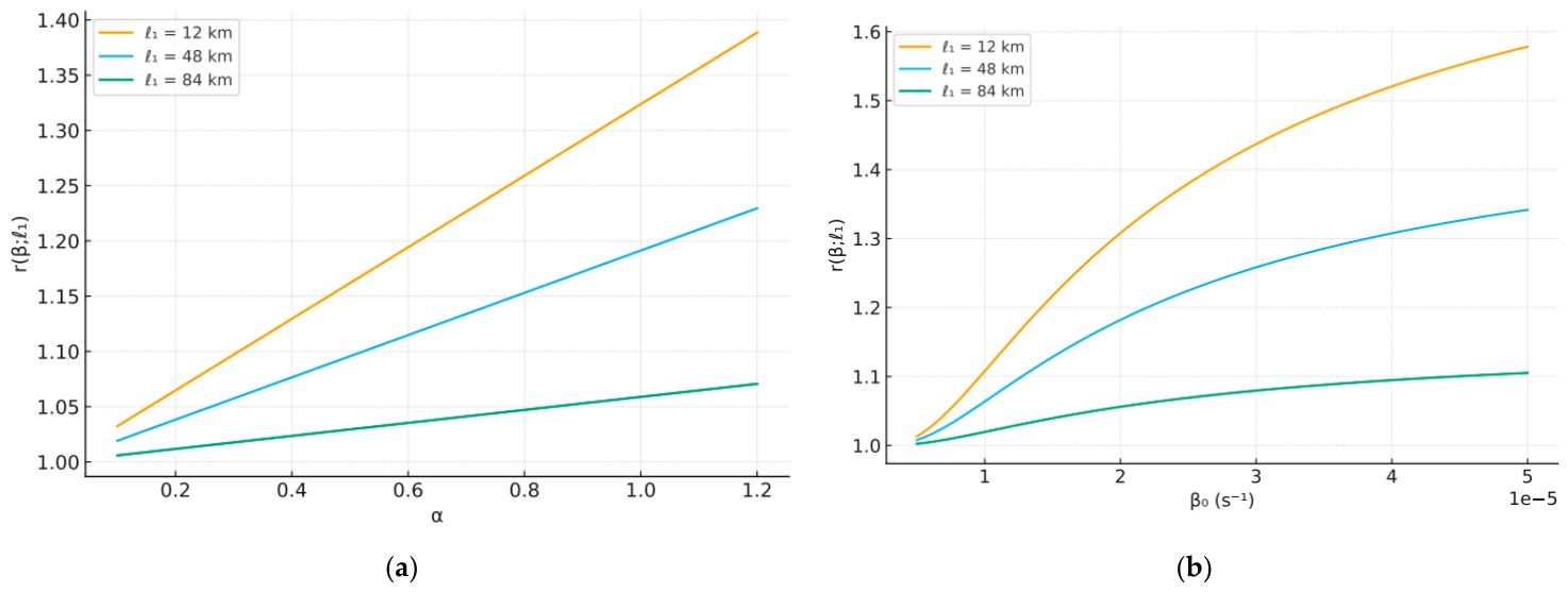
Variation in the leakage amplification factor r(β;ℓ₁) with respect to the amplification parameter α for three representative leak locations (ℓ₁ = 12, 48, 84 km). The figure is intended to illustrate the influence of leak position on the amplification factor under identical attenuation conditions. Calculations were performed using L = 100 km, β = β₀ = 2.1 × 10⁻⁵ s⁻¹, while α was varied within the 0.1 ≤ α ≤ 1.2.

Sensitivity of the leakage amplification factor r(β;ℓ₁) to the attenuation scale β₀. The figure illustrates the attenuation-dependent behavior and boundedness of the proposed representation. Calculations were performed for L = 100 km, α = 1.0, and β = 2.1 × 10⁻⁵ s⁻¹.

Figure A2a,b illustrates the variation in r(β;ℓ₁) for representative leak locations and attenuation levels. The results demonstrate that:

• Upstream leaks produce the largest amplification factors;
• Downstream leaks exhibit the weakest hydraulic influence;
• The amplification factor decreases monotonically with increasing attenuation;
• The function remains bounded and physically meaningful over the entire parameter range.

Consequently, r(β;ℓ₁) provides a compact and physically interpretable representation of the influence of leak location and attenuation on transient leakage intensity while preserving the analytical structure of the governing model.

Figure A2. (a). Dependence of the leakage amplification factor r(β;ℓ₁) on the amplification parameter α for representative leak locations. (b). Dependence of the leakage amplification factor r(β;ℓ₁) on the reference attenuation scale β₀.

Figure A2. (a). Dependence of the leakage amplification factor r(β;ℓ₁) on the amplification parameter α for representative leak locations. (b). Dependence of the leakage amplification factor r(β;ℓ₁) on the reference attenuation scale β₀.

References

- Zhao, T.; Shin, B.R. Upwind scheme using preconditioned artificial dissipation for unsteady gas-liquid two-phase flow and its application to shock tube flow. J. Appl. Fluid Mech. 2024, 17, 1806–1819. [Google Scholar] [CrossRef] [Scilit]
- Luo, X.; Yang, R.; Wu, Q.; Zhang, D. Hydraulic transient analysis in low gas-liquid ratio pipelines under valve closure conditions: Pressure surge characteristics and predictive modeling. J. Pipeline Sci. Eng. 2026, 6, 100376. [Google Scholar] [CrossRef] [Scilit]
- Thorley, A.R.D. Fluid Transients in Pipeline Systems; Professional Engineering Publishing: London, UK, 2004. [Google Scholar]
- Wylie, E.B.; Streeter, V.L. Fluid Transients in Systems; Prentice Hall: Hoboken, NJ, USA, 1993. [Google Scholar]
- API. Recommended Practice 14E: Design and Installation of Offshore Production Platform Piping Systems; American Petroleum Institute: Washington, DC, USA, 2013. [Google Scholar]
- ISO 13623; Petroleum and Natural Gas Industries—Pipeline Transportation Systems. International Organization for Standardization: Geneva, Switzerland, 2017.
- IGEM. IGEM/TD/1: Steel Pipelines for High Pressure Gas Transmission; Institution of Gas Engineers and Managers: London, UK, 2020. [Google Scholar]
- Zhao, Y.; Tao, X.; Li, L.; Guo, Z.; Qi, H.; Wang, J.; Yang, K.; Lin, W.; Fan, J.; Chen, C. Assessment of the Measured Mixing Time in a Water Model of Asymmetrical Gas-Stirred Ladle with a Low Gas Flowrate Part II: Effect of the Salt Solution Tracer Volume and Concentration. Symmetry 2025, 17, 802. [Google Scholar] [CrossRef] [Scilit]
- Shen, Y.; Chu, W.; Chen, J. Seal leakage flow-affected compressor endwall and fillet profiling design based on optimization and data mining. J. Appl. Fluid Mech. 2026, 19, 1449–1468. [Google Scholar] [CrossRef] [Scilit]
- Kappes, M.A.; Larrosa, N.O.; Bergant, M.A.; Perez, T.E. Blending hydrogen in existing natural gas pipelines: Impact of reduced JR-Curve slope on the pipeline integrity. Int. Eng. Fail. Anal. 2026, 186, 110517. [Google Scholar] [CrossRef] [Scilit]
- Aliyev, I.G.; Gafarbayli, K.A.; Mammadov, A.; Mammadrazayeva, F. Unsteady gas dynamics modeling for leakage detection in parallel pipelines. Coupled Syst. Mech. 2025, 14, 371–393. [Google Scholar] [CrossRef]
- IEA. Global Hydrogen Review; International Energy Agency: Paris, France, 2023. [Google Scholar]
- Zhang, K.; Ma, R.; Geng, T.; Yang, J.; Hou, J. Leakage detection method based on transient pressure behaviors during pigging process in pipelines. Measurement 2025, 240, 115598. [Google Scholar] [CrossRef] [Scilit]
- Yu, J.; Yi, J.; Mahgerefteh, H. Optimal emergency shutdown valve configuration for pressurised pipelines. Process Saf. Environ. Prot. 2022, 159, 768–778. [Google Scholar] [CrossRef] [Scilit]
- Sundar, K.; Zlotnik, A. State and Parameter Estimation for Natural Gas Pipeline Networks Using Transient State Data. IEEE Trans. Control Syst. Technol. 2018, 27, 2110–2124. [Google Scholar] [CrossRef] [Scilit]
- Chaczykowski, M. Transient flow in natural gas pipeline systems. Appl. Math. Model. 2010, 34, 1051–1067. [Google Scholar] [CrossRef] [Scilit]
- Yuan, W.; Chen, Z.; Zhao, G.; Su, C.; Kong, B. Semi-Analytical Reservoir Modeling of Non-Linear Gas Diffusion with Gas Desorption Applied to the Horn River Basin Shale Gas Play, British Columbia (Canada). Energies 2024, 17, 676. [Google Scholar] [CrossRef] [Scilit]
- Mammadov, A.; Mammadrzayeva, F.; Aliyev, I.G. Analytical and Asymptotic Modeling of Coupled Transient Gas Redistribution Induced by Simultaneous Injection and Withdrawal in Transmission Pipelines. Math. Comput. Appl. 2026, 31, 103. [Google Scholar] [CrossRef] [Scilit]
Disclaimer/Publisher’s Note: The statements, opinions and data contained in all publications are solely those of the individual author(s) and contributor(s) and not of MDPI and/or the editor(s). MDPI and/or the editor(s) disclaim responsibility for any injury to people or property resulting from any ideas, methods, instructions or products referred to in the content. |
© 2026 by the authors. Licensee MDPI, Basel, Switzerland. This article is an open access article distributed under the terms and conditions of the Creative Commons Attribution (CC BY) license.