


Abstract
Predicting systemic stress in high-dimensional equity markets remains challenging, owing to non-stationarity, heavy tails, and regime shifts. This paper introduces GWS-STNet (Gaussian-Weighted Swin Spatio-Temporal Network), a deep learning architecture grounded in functional analysis and thermodynamic analogy. A Gaussian-Weighted Swin Operator () replaces the standard shifted-window attention mechanism with a kernel-regularised counterpart on the Hilbert space () of financial spatio-temporal voxels. The principal theoretical contribution is a proof, via the Banach Fixed-Point Theorem, that the window-level attention operator () is a strict contraction (Lipschitz constant of ) under a bandwidth of , guaranteeing convergence of internal network representations to a unique fixed point. Metabolic Saliency (), derived from the exact Jacobian of the Power Mapping Network (PMNet) weighted by pairwise transfer entropy, provides intrinsic, post hoc-free attribution of sector-level stress contributions. Empirical validation on 15 large-capitalisation JSE securities ( trading days, January 2015–December 2025) with Eskom load-shedding stages as exogenous stress injectors shows that GWS-STNet outperforms nine baselines, including classical benchmarks (Random Walk and AR(1)) and state-of-the-art Transformers across RMSE, MAE, the Gaussian Calibration Score (GCS), and the Metabolic Efficiency Ratio (MER), with Diebold–Mariano .
1. Introduction
Financial market modelling sits at an unresolved boundary. On one side stands a half-century of linear econometrics: the ARIMA family of Box and Jenkins [1] remains the workhorse of applied forecasting precisely because its parameters carry direct probabilistic meaning and its inference is well-understood. The cost is visible in any JSE return series displaying volatility clustering or a fat-tailed distribution that the Gaussian assumption cannot accommodate [2]. On the other side, recurrent and Transformer architectures have closed the accuracy gap on standard benchmarks substantially [3,4]. What they have not provided is any assurance that the accuracy survives a regime shift. A model calibrated on a tranquil 2016 quarter and deployed through a Stage 6 load-shedding crisis in 2022 carries no certificate of stability: its internal dynamics may amplify rather than absorb the shock. That gap between a model that performs well on average and one whose behaviour is bounded under stress is what this paper addresses.
Attention mechanisms, as introduced by Vaswani et al. [5], represent a departure from the sequential inductive bias of recurrent networks. The Swin Transformer [6] advanced the field by introducing hierarchical, shifted-window attention that captures both local and long-range spatial dependencies with linear computational complexity, properties that are attractive for financial spatio-temporal modelling, where sectoral correlations evolve in a manner analogous to spatial proximity in image data. However, the Swin Transformer carries no mechanism for handling the non-stationary entropy production characteristic of financial stress episodes; applied to equity panels, its attention heads exhibit gradient instability under high-volatility conditions, rendering standard architectures unreliable precisely when robustness is most required [7].
1.1. The Metabolic Gap in Financial Econometrics
Positioning within the systemic risk literature. The financial systemic-risk literature provides important benchmarks for the present framework. Billio et al. [8] demonstrated that Granger-causal network connectivity among financial institutions predicts systemic crises, establishing the network-theoretic foundation that GWS-STNet extends to the spatio-temporal domain. Adrian and Brunnermeier [9] showed that CoVaR, value at risk conditional on a financial institution being in distress, captures cross-sectional risk spillovers; metabolic saliency serves an analogous attribution function at the sector level. Diebold and Yilmaz [10] developed variance decomposition network measures of financial connectedness; both their approach and the transfer-entropy formulation proposed here quantify directional information flow between financial entities, but transfer entropy is non-parametric and captures nonlinear dependence, making it more appropriate for regime-switching JSE return series [11]. GWS-STNet contributes to this literature by providing a deep learning architecture that detects the dynamics of systemic stress propagation rather than static connectedness.
Scope of the metabolic analogy. Terms such as “metabolic stress”, “capital flux”, and “entropy production” are used throughout as disciplined analogies to non-equilibrium thermodynamics [12]. No claim is made that financial markets obey physical conservation laws. The thermodynamic vocabulary motivates the loss-function design and the stress-indicator construction; the core contribution is the Gaussian-weighted attention operator, its provable contractive behaviour, and the metabolic saliency attribution metric. A formal connection to the Fokker–Planck equation is left for future work.
The gap that motivates this paper is architectural. Deep learning models deployed in finance treat market stress as a statistical residual: if a model calibrated on 2015–2018 JSE data encounters a Stage 6 load-shedding event in 2022, nothing in its architecture constrains how its internal representations respond. Predictive accuracy during tranquil periods carries no guarantee of coherent behaviour during the tail events that determine portfolio survival. Physics offers a different approach. Non-equilibrium thermodynamic systems self-organise through entropy production [12], and a market under severe infrastructure stress exhibits precisely this character: correlations spike, sector relationships reorganise, and the information geometry of the state space deforms in ways that standard volatility models do not capture. The question is not whether this analogy is perfect but whether embedding it in an architecture produces a model whose behaviour is provably bounded under stress rather than empirically stable on average.
The JSE provides a sharper test of this question than any mature-market dataset can. Eskom load-shedding stages are fully exogenous to equity-market microstructure: their timing and severity are determined by generation-capacity constraints, not by financial conditions [13]. Each stage change is a quantified energy shock whose transmission across the sector network is traceable in the price and volume data. No equivalent instrument exists in European or North American equity panels. The decade-long JSE record used here covers Stage 1 through Stage 6 episodes, two complete business cycles, the COVID-19 disruption, and the 2022–2023 peak curtailment crisis, providing the distributional range needed to test whether architectural-stability guarantees hold under qualitatively different stress regimes.
1.2. From Black Box to Intrinsic Interpretability
The standard response to the black-box problem in financial machine learning has been post hoc: train a model, then approximate its behaviour locally using SHAP [14] or Grad-CAM [15] to generate attribution scores. Slack et al. [16] demonstrated that both methods can be adversarially manipulated to produce attribution rankings that bear no relationship to the model’s actual computational graph, without any detectable change in predictive output. Adebayo et al. [17] showed that several widely used saliency maps fail basic sanity checks: randomising the model’s weights leaves the attributions nearly unchanged. The failure mode is structural. Post hoc methods approximate the model at a point; they provide no certificate that the approximation holds elsewhere and no guarantee that the attribution is stable when the model is retrained on a different data split.
Contraction mapping provides an entirely different foundation. If the operator governing the model’s internal representations is a strict contraction, then the model possesses a unique fixed point to which all trajectories converge geometrically. Perturbations in input do not amplify through the layers; the model’s behaviour is bounded by construction rather than calibrated on historical data. This topological property is the starting point for intrinsic interpretability: when the architecture is stable by design, the Jacobian of its output with respect to its input is a meaningful and bounded quantity at every point in the input space, not just near the training distribution.
Metabolic saliency () is built on this foundation. Rather than approximating a trained model after the fact, is defined as the exact Jacobian of the Power Mapping Network output with respect to each input voxel, weighted by the pairwise transfer entropy between sectors [18]. Transfer entropy measures directed information flow: the degree to which the past of sector (j) reduces uncertainty about the future of sector i beyond what sector i’s own history provides. Weighting the Jacobian by this quantity converts a gradient map into a directional information-flux attribution. The result is an attribution metric that is exact rather than approximate, grounded in information geometry [19] rather than local linear surrogates, and stable under retraining by Definition 11 rather than by empirical convention.
1.3. Contributions
This paper makes four contributions to the literature on statistical deep learning and financial econometrics.
- (i)
- Topological stability guarantee via contractive attention: The Gaussian-Weighted Swin Operator () is proven to be a strict contraction mapping on the complete metric space of financial spatio-temporal voxels under a bandwidth constraint of , with convergence to a unique metabolic equilibrium guaranteed by the Banach Fixed-Point Theorem. The theoretical boundary is verified empirically through a bandwidth-sensitivity ablation that confirms a sharp phase transition in contractivity at . The threshold of is a sufficient condition for contractivity of the attention operator, derived from the spectral attenuation bound in Lemma 2; it is not claimed to be necessary. A complete proof for the full nonlinear residual architecture remains an open problem [20].
- (ii)
- Intrinsic interpretability via metabolic saliency: Grounded in the information-geometric framework of Amari [19] and the transfer entropy of Schreiber [18], metabolic saliency () is introduced as an attribution metric derived directly from the PMNet Jacobian weighted by pairwise sector-transfer entropy. Unlike SHAP [14] and LIME [21], is architecturally intrinsic, faithful in the sense of Definition 11, and stable under retraining. Corollary 2 establishes that sector rankings are reproducible across retraining runs, satisfying the auditability requirements of FSRA [22] and MiFID II [23].
- (iii)
- Novel evaluation metrics: Standard RMSE and MAE measure average prediction error but are insensitive to distributional drift under stress. Two metrics are introduced to fill this gap. The Gaussian Calibration Score (GCS) measures how closely the model’s residual distribution tracks the Gaussian equilibrium estimated on the training baseline using the squared 2-Wasserstein distance [24]. The Metabolic Efficiency Ratio (MER) captures the trade-off between predictive accuracy and the entropy level at which that accuracy is achieved, extending the efficiency paradigm of [25] to account for model-internal metabolic cost.
- (iv)
- Empirical emerging-market application: The framework is validated on the JSE canonical panel (15 large-capitalisation JSE securities; trading days, January 2015 to December 2025) with Eskom load-shedding stages as exogenous metabolic stress injectors [13]. South Africa’s infrastructure crisis provides a natural experiment unavailable in mature-market data: exogenous, stage-quantified energy shocks whose transmission across the equity network is traceable sector by sector. The empirical design addresses the gap identified in Table 1: no prior architecture simultaneously provides a stability certificate, intrinsic interpretability, and validation under infrastructure-driven emerging-market stress.
1.4. Paper Organization
Section 3 establishes mathematical preliminaries: the spatio-temporal voxel space, the metabolic state function, and the Gaussian-weighted Swin operator. Section 4 presents the GWS-STNet and PMNet architectures, together with the metabolic loss function. Section 5 states and proves Theorem 2 (contraction mapping) and introduces metabolic saliency and the Saliency–Entropy Duality Theorem. Section 6 describes the JSE-Eskom dataset, the experimental protocol, and the proposed evaluation metrics. Section 7 presents empirical results. Section 8 discusses implications for portfolio risk management. Section 9 concludes this work and outlines future directions with respect to information-theoretic mapping.
2. Related Work and Literature Positioning
A rigorous positioning of the GWS-STNet framework requires the synthesis of three distinct but interacting research streams: (i) physics-informed and thermodynamic approaches to financial modelling, (ii) Transformer architectures and their stability properties, and (iii) interpretability and attribution in financial deep learning. Table 1 provides a structured mapping of the 20 most closely related papers across these streams against the seven defining features of the present contribution.
2.1. Stream 1: Physics-Informed Financial Modelling
Physics entered financial modelling not through analogy but through observation. Mandelbrot [26] noticed that cotton price changes scaled in the same way as turbulent fluid flows, a fractal signature incompatible with any Gaussian model. Cont [2] later documented this pattern systematically across equity markets: fat tails, volatility clustering, and long memory appeared with sufficient regularity across markets and time periods to be treated as empirical constraints rather than anomalies. Stanley et al. [27] pushed the connection further, showing that methods from statistical mechanics, particularly the study of phase transitions near critical points, reproduced the scaling properties documented by Mandelbrot and Cont, without requiring them as assumptions. The thermodynamic foundation came from Prigogine and Nicolis [12]: dissipative systems far from equilibrium self-organise through entropy production, and a stressed financial market, with capital fleeing sector by sector and correlations spiking simultaneously, displays exactly this character. What the physics-informed literature did not do is embed these principles inside a neural architecture. Physical concepts appeared in loss functions or as post hoc descriptions; no published model inherits a topological stability property from a physical constraint. That is the first gap this paper closes.
What the physics-informed finance literature has not achieved is the embedding of these thermodynamic principles directly into the architecture of a deep learning model. Papers in this stream use physical concepts as descriptive tools or as loss-function constraints [28], but none proves that the resulting neural operator inherits a topological stability property (such as contractivity) from the physical constraint. This is the first gap addressed by the present paper.
2.2. Stream 2: Transformer Architectures and Stability
The Transformer [5] and its hierarchical variant, the Swin Transformer [6], have become the dominant architectures for sequence and image modelling. Their application to financial time-series forecasting has been explored by the Informer [4] (ProbSparse attention for long sequences), Autoformer [29] (series decomposition with auto-correlation attention), and Patchtst [30] (patch-based tokenisation for multivariate series) models. These models achieve state-of-the-art predictive accuracy on standard benchmarks but share a critical limitation: none provides a mathematical stability guarantee for the attention mechanism under distributional shift, i.e., when the test distribution diverges substantially from the training distribution, as occurs during financial stress episodes [7].
The mathematical stability of neural operators has been studied in the context of Lipschitz-constrained networks [31], invertible residual networks [32], and the general contraction framework for recurrent networks. Vuckovic et al. [20] studied the universal approximation and stability properties of self-attention operators but did not connect stability to a specific architectural constraint (such as a Gaussian kernel) or to a financial application. The present paper fills this gap by proving a conjectured contraction property for the Gaussian-masked Swin operator under an explicit bandwidth condition and verifying it empirically on the JSE panel.
2.3. Stream 3: Interpretability in Financial Deep Learning
The interpretability of deep learning models in finance has been pursued through gradient-based saliency maps [15], SHAP values [14], and LIME [21]. Bianchi et al. [33] applied Fisher information to construct interpretable bond-risk premia. Gu et al. [34] used information-theoretic methods for factor-model selection. Adebayo et al. [17] demonstrated that widely used saliency methods fail basic sanity checks, and Slack et al. [16] showed that SHAP and LIME can be adversarially manipulated without affecting model predictions.
The common limitation of these approaches is the absence of a statistical convergence guarantee: none proves that its attribution metric converges to a well-defined population quantity as the sample size grows, and none connects the attribution to a physically interpretable unit (such as bits of information per trading day). The metabolic saliency introduced here and formally connected to KL divergence in [35] addresses both gaps.
2.4. Literature-Gap Map
Table 1 synthesises the three streams. Columns represent the seven defining features of the GWS-STNet framework; rows represent the 20 most closely related papers. A filled circle (•) indicates the paper fully addresses the feature; a half circle (∘) indicates partial treatment; a dash (,) indicates the feature is absent.
Table 1.
Literature-gap map: 20 representative papers across three research streams vs. the seven features of the GWS-STNet framework. Features: (F1) physics-informed loss or architecture; (F2) topological stability guarantee; (F3) emerging-market application; (F4) intrinsic (non-post hoc) interpretability; (F5) transfer-entropy attribution; (F6) infrastructure shock as exogenous stress variable; (F7) Convergence guarantee for attribution metric.
Synthesis. Table 1 reveals three convergences and three divergences in the literature. The convergences are: (i) physics-informed methods (Stream 1) and stability-focused Transformer work (Stream 2) both recognize that standard deep learning is fragile under distributional shift, motivating architectural constraints; (ii) Stream 3 papers universally acknowledge that post hoc interpretability is insufficient for regulatory purposes, motivating intrinsic methods; and (iii) the econophysics literature (Stanley et al. [27], Schreiber [18], Barnett et al. [36]) converges on transfer entropy as the most principled measure of directed information flow in financial networks. The divergences are: (i) physics-informed methods do not prove topological stability, as no paper in Stream 1 contains a contraction theorem; (ii) stability-focused Transformer work (Stream 2) does not address financial applications or emerging-market infrastructure shocks; and (iii) no paper in any stream simultaneously addresses all seven features (F1–F7). The GWS-STNet framework is the only one in Table 1 to address all seven features simultaneously.
3. Mathematical Preliminaries
The framework is built on a hierarchy of mathematical objects: a probability space, a function space of market states, a spatio-temporal voxel representation, and the operator that acts on it. Each object is defined precisely before the theorem is stated.
3.1. Foundational Probability Space
The mathematical foundation of GWS-STNet rests on a measure-theoretic probability space that accommodates the inherent randomness of financial returns while providing a sufficiently rich structure for the operator theory developed in Section 5. Following the standard construction of continuous-time financial models, we work on a filtered probability space that satisfies the “usual conditions” (completeness and right continuity of the filtration) that are necessary for the application of martingale theory and stochastic integration. The discrete index set () reflects the practical reality that JSE equity prices are observed at daily closing auctions rather than in continuous time; the panel spans a full decade, including two complete business cycles, three national elections, the COVID-19 pandemic, and the peak Eskom load-shedding crisis of 2022–2023, providing the distributional breadth required to stress-test the contraction property across qualitatively distinct market regimes.
Definition 1
(Filtered probability space). Let be a complete probability space equipped with a right-continuous filtration () satisfying the usual conditions. All random objects in this paper are defined on . The discrete-time index set (, where ) denotes the set of JSE trading days over the period from 5 January 2015 to 29 December 2025. For each , the sigma algebra () represents the information available to a market participant at the close of day t and includes all price and volume history up to and including day t, as well as the Eskom load-shedding stage () announced before market open.
3.2. The Spatio-Temporal Voxel Space
The representation of financial panel data as a three-dimensional tensor (securities × features × time) follows the spatio-temporal data-cube paradigm established in the computer vision literature and adapted to financial networks by Jiang et al. [37]. The choice of three feature channels—log return, volume, and realised variance—is grounded in the stylised facts of equity markets documented by Cont [2]: these three variables jointly capture the first and second moments of the return distribution and the market’s trading intensity, which, together, determine the information content of each trading day. Realised variance is computed as a 21-day rolling window following the realised volatility literature of Andersen et al. [38].
Definition 2
(Spatio-temporal voxel). Let with index the set of large-capitalisation JSE securities, and let with index the following feature channels, each standardised to zero mean and unit variance in-sample: log return (), turnover-adjusted volume (), and realised variance ( [38]). A spatio-temporal voxel at time t and in sector i is expressed as the following triple:
The full data tensor at time t over a rolling window of length τ is
Definition 3
(Voxel Hilbert space). The Hilbert space is defined as
equipped with an inner product expressed as and an induced norm expressed as . The metric expressed as makes a complete metric space.
3.3. The Metabolic State Function
The metabolic state function formalizes the thermodynamic analogy between biological energy flux and financial capital flux. In non-equilibrium thermodynamics [12], the energy dissipated by a system per unit of time is the product of a generalized force and a generalized flux. The financial analogue, following the econophysics literature of Stanley et al. [27] and Mantegna and Stanley [39], treats price movement as the “force” and share volume as the “flux”: their product () measures the capital work performed by the market to move security i by return . This is dimensionally analogous to mechanical power (force times velocity) and was first applied to equity markets by Lo and Wang [40] under the name of “turnover-adjusted return.”
The Shannon entropy term [41] captures a distinct dimension of metabolic stress: the informational disorder of the return distribution. High entropy indicates that returns are spread uniformly across the histogram bins, reflecting uncertainty or unpredictability, consistent with a market in stress; low entropy indicates a concentrated, predictable distribution characteristic of the resting state. Combining flux and entropy into a single metabolic state function follows the approach of Gençay et al. [42], who showed that joint volume–return measures provide superior early-warning signals for market-regime transitions compared to either measure alone.
Definition 4
(Capital flux and metabolic state). The capital flux of security i at time t is defined as
representing the volume-weighted magnitude of price change, i.e., the “work done” by the market to move security i by return [40].
The metabolic state function () is defined by
where is the instantaneous Shannon entropy [41] of the empirical return distribution of security i within the rolling window (τ):
with representing the probability mass in the b-th bin of a B-bin histogram of [43]. Periods of high signal metabolic stress in security i: elevated energy dissipation coupled with informational disorder.
Definition 5
(Exogenous metabolic stress indicator). Let denote the Eskom load-shedding stage recorded on trading day t, where stage 0 indicates no shedding and stage 6 corresponds to the maximum recorded curtailment. The augmented metabolic state is
where is a coupling parameter and is the energy-intensity weight of sector i, estimated from JSE-sector GICS classifications.
3.4. The Gaussian-Weighted Swin Operator
We now define the central object of the paper. The standard Swin attention mechanism partitions the feature map into non-overlapping windows of size and computes self-attention within each window, then shifts the partition by in the subsequent layer to allow for cross-window information exchange [6]. This paper replaces the uniform window weighting with a Gaussian kernel.
Definition 6
(Gaussian kernel on the voxel lattice). Let denote a lattice coordinate (sector, time). For a bandwidth of , the Gaussian attention kernel is
The kernel is symmetric and positive definite and satisfies for all .
Definition 7
(Gaussian-Weighted Swin Operator). For a query–key–value triple derived from a voxel tensor () via learnable projections (), the Gaussian-Weighted Swin Operator () acts within each Swin window () as
where is the key dimension introduced by Vaswani et al. [5], acting as the scaling factor that prevents the dot-product from entering the saturating region of the softmax; is the output projection; ⊙ denotes the Hadamard (element-wise) product [19]; and is the Gaussian attention mask with entries , renormalized so that each row sums to unity. The standard Swin self-attention formulation of Liu et al. [6] corresponds to the special case of (uniform weighting); the Gaussian mask is a strictly more expressive generalization that introduces a spatial prior reflecting the metabolic coupling structure of the JSE sector network.
Remark 1.
The Gaussian mask () encodes a spatial prior that penalizes attention between distant lattice points proportionally to their Euclidean separation. In the financial context, this represents the metabolic principle that stress propagation between sectors is distance-decaying: a shock originating in the energy sector diffuses into adjacent industrial and utility sectors before reaching financial services, with coupling strength governed by σ.
Lemma 1
(Boundedness of Swin attention). Let be the standard self-attention matrix computed within a Swin window. Then, for all and for all m. Consequently, and , where denotes the window cardinality.
Proof.
The softmax function maps any real vector to the probability simplex (), so and for every row m. Row stochasticity implies . The Frobenius bound follows from , where the last inequality uses , since . □
Lemma 2
(Gaussian smoothing attenuates high-frequency entropy). Let , and let denote the convolution of f with the Gaussian kernel (). Then, in the Fourier domain,
so high-frequency components ( large) are attenuated exponentially in . In particular, the power spectral density satisfies .
Proof.
The Fourier transform of a Gaussian convolution kernel satisfies (see, e.g.,). The convolution theorem then gives , from which the stated bound follows immediately by taking squared moduli. □
Remark 2.
Lemma 2 provides the statistical justification for the Gaussian mask in Definition 7: by suppressing high-frequency components of the attention weight tensor, functions as a spectral low-pass filter, attenuating the “entropy noise” generated by short-duration volatility spikes whilst preserving the structural, low-frequency sectoral correlation patterns that drive systemic risk.
Assumption 1
(Metabolic state as a semimartingale). For each sector , the metabolic state process () is a continuous-time semimartingale with respect to the filtration (), satisfying
where is a standard Brownian motion on , is a pure jump process capturing exogenous infrastructure shocks (Eskom stage transitions and settlement-platform outages), and and are -predictable processes satisfying a.s. for all . The discrete-time observations () are the daily closing values on the business-day grid ().
Remark 3.
The semimartingale structure is the minimal regularity that supports Itô calculus and is consistent with the standard no-arbitrage framework of semimartingale asset-price models. The jump component () is not a modelling convenience but a thermodynamic necessity: Eskom stage changes represent abrupt reductions in available coordination energy that cannot be represented by a continuous diffusion. Discrete-time GWS-STNet operates on a Euler discretisation of (2) at the one-day scale; the semimartingale assumption justifies the use of standard time-series asymptotics for the convergence analysis in Section 5.1.
Reconciliation with predictability. A subtlety arises regarding the coexistence of the semimartingale assumption and the forecasting objective. Under the risk-neutral measure (), the no-arbitrage framework requires discounted asset prices to be local martingales, which would preclude systematic predictability. However, the GWS-STNet operates under the physical (statistical) measure (), not . Under , the drift () in (2) need not be zero; systematic predictability in the form of non-trivial conditional expectations is fully consistent with the semimartingale structure [44]. The transfer entropy () in Definition 9 captures -measure dependence between sector-return processes, not -measure martingale residuals. Therefore, GWS-STNet’s predictive advantage does not contradict the semimartingale framework: no-arbitrage constrains , while the model exploits -measure drift and cross-sectional dependence structures.
4. The GWS-STNet and PMNet Architectures
The GWS-STNet architecture translates the mathematical objects of Section 3 into a concrete computational graph. Following the hierarchical design principle of Liu et al. [6], the architecture operates in four stages of progressively coarser spatio-temporal resolution, with the Gaussian-Weighted Swin Operator (; Definition 7) replacing the standard shifted-window attention at each stage. The Power Mapping Network (PMNet) then maps the bottleneck representation to sector-level metabolic power scores, and the metabolic loss function (Section 4.4) closes the training loop. Figure 1 provides a schematic overview of the complete pipeline.
Figure 1.
Overview of the GWS-STNet architecture. The input voxel () is patch-embedded and processed through four Gaussian-Weighted Swin Transformer Block (GWSTB) stages of progressively coarser resolution. The bottleneck () feeds the Power Mapping Network (PMNet), producing metabolic power scores (). The dashed red arrow denotes saliency backpropagation pass computing () with no additional forward pass. Spectral normalization () is enforced on all projection matrices (Assumption 2).
4.1. GWS-STNet: Multi-Scale Spatio-Temporal Encoding
GWS-STNet is a four-stage hierarchical encoder following the general Swin backbone [6], modified to operate on 3D financial voxel tensors and to replace uniform window attention with . The four stages are described below.
Input representation. The input tensor () is partitioned into non-overlapping spatio-temporal patches of size (sector stride × time stride), each embedded into a d-dimensional vector via a linear patch embedding ().
Four-stage hierarchy. At each stage (), the feature map is processed by a sequence of GWS Transformer Blocks (GWSTBs), followed by a patch-merging layer that halves the spatial resolution and doubles the channel depth:
GWSTB. Each block applies, in succession, layer normalization, the Gaussian-Weighted Swin Operator (, alternating standard and shifted windows), a residual connection, a second layer normalization, and a two-layer feed-forward network with GELU activation:
4.2. Power Mapping Network (PMNet)
The Power Mapping Network (PMNet) translates the high-dimensional bottleneck representation produced by the GWS-STNet encoder into a sector-level metabolic power score. For a self-contained presentation, the PMNet target variables are defined here. The metabolic state of sector i at time t is , where is the conditional expected log return and is the GICS energy-intensity weight for sector i. The entropy production rate is , where is the training-baseline mean metabolic state. These two quantities are the PMNet decoder targets; they are originally introduced in the companion paper [35] but are reproduced here for completeness. The concept of a “power map” is grounded in the physics of energy dissipation: in thermodynamic systems, power is the rate at which energy is transferred, and a mapping from internal state to power output describes how efficiently the system converts stored information into a useful work signal [12]. In the financial context, the PMNet quantifies the “work done” by the market to sustain its current price configuration; sectors exhibiting high power scores are those whose price movements demand large capital mobilisation relative to the informational content of the change, which is the hallmark of metabolic stress.
Architecturally, the PMNet is a three-layer multi-layer perceptron (MLP) with Gaussian Error Linear Unit (GELU) activations [45]. The GELU activation (, where is the standard Gaussian cumulative distribution function) is preferred over ReLU in this setting because it is infinitely differentiable, ensuring that the Jacobian () required for the metabolic saliency computation (Definition 10) is well-defined everywhere. The spectral normalization of each weight matrix (; Section 5, Step 2 of the proof) is applied to the PMNet layers, as well as to the GWS-STNet attention projections, ensuring that the Lipschitz bound () is maintained throughout the full forward pass [31].
Definition 8
(PMNet power mapping). The PMNet () maps the Stage-4 bottleneck representation () to a sector-level metabolic power score :
with , , , and corresponding bias vectors. The PMNet output () approximates for the target trading day () at forecast horizon h, where is the augmented metabolic state of Definition 5.
4.3. Information Geometry of the PMNet Residual Manifold
The theoretical justification for the metabolic loss function rests on the information-geometric structure of the PMNet residuals. Let denote the residual for sector i at time t and suppose the conditional distribution of , given the hidden state (), belongs to a regular exponential family [19]:
where is the natural parameter, is the sufficient statistic, and is the log-partition function. The Fisher information matrix at parameter is
where the second equality follows from the standard identity for exponential families [19]. The family defines a statistical manifold (, where is the Fisher–Rao Riemannian metric).
The KL divergence between the stressed distribution () and the resting baseline () admits the following second-order approximation:
where is the parameter displacement from the resting state. Equation (8) is the foundation for the KL-divergence metabolic saliency estimator in [35]: the saliency weight () approximates the information-geometric distance () between the crisis and resting parameter vectors. The exponential family assumption is assessed empirically via Kolmogorov–Smirnov tests reported in the empirical results of Section 6.
4.4. Metabolic Loss Function
Standard mean squared error treats a prediction failure in January 2016, when JSE volatility was near its decade low, identically to a failure in July 2022, when Stage 6 load-shedding was driving coordinated sector drawdowns across all 15 large-cap securities simultaneously. That treatment is wrong for a framework grounded in non-equilibrium thermodynamics. The Second Law is explicit on this point [12]: entropy production accelerates as a system moves away from equilibrium, so the informational cost of a misprediction grows with the entropy of the state in which it occurs. A model that underestimates stress during a metabolic crisis does not merely incur a larger squared error; it fails at the moment when the systemic consequences of prediction error are largest. The loss function must reflect this asymmetry. Therefore, an entropy-weighted penalty that scales exponentially with the instantaneous system entropy () is introduced so that errors committed during high-entropy regimes are penalised more severely than arithmetically equivalent errors during resting periods.
The Kullback–Leibler (KL) divergence regularizer [46] serves a complementary function: it constrains the distribution of PMNet residuals to remain close to a Gaussian equilibrium () estimated on the training set. This is the information-theoretic operationalisation of the metabolic homeostasis concept; the model is penalized for allowing its error distribution to drift from the “resting state”. The Gaussian target () is justified by Lemma 2, which establishes that the Gaussian kernel attenuates high-frequency spectral components of the attention weight tensor; the resulting residuals inherit a quasi-Gaussian character under contractivity. The complete loss function is expressed as follows:
where is the mean system entropy at time t [41], are hyperparameters tuned via Bayesian optimization on the walk-forward validation set; is the empirical distribution of the PMNet residuals at each training step, and is the Gaussian equilibrium distribution estimated on the training baseline. The information-geometric development in Section 5 assumes an exponential family structure for the residuals in the neighbourhood of . This is a local approximation: the JSE return series exhibit heavy tails globally (excess kurtosis: ), but the residuals of the fitted model are substantially closer to Gaussian in low-stress windows, justifying the local exponential family approximation [19]. Results depending on this approximation should be understood as a local rather than global distribution estimated on the in-sample training baseline (January 2015 to December 2018). The exponential weighting function () is a direct adaptation of the importance-weighted loss framework of Shimodaira: whereas Shimodaira reweights by density ratio to correct for covariate shift, here, we reweight by entropy to correct for regime shift, penalising the model more severely for errors occurring in the high-entropy tail of the data distribution. The two hyperparameters are calibrated jointly on the walk-forward set; the ablation in Table 5 (reported in Section 7.1) confirms that setting degrades GCS from to , quantifying the loss of metabolic awareness.
Theorem 1
(Generalisation bound for the metabolic loss). Let be the metabolic loss (Section 4.4) with an entropy weight of and a KL regularisation term. The PMNet hypothesis class is denoted by , and is its empirical Rademacher complexity over training examples. The following bound is established under the α-mixing condition (C2) of Section 6.1, which ensures that Rademacher complexity arguments extend from the i.i.d. setting to dependent time series via the blocking technique of Yu [47]. Under (C2), the effective sample size is , where is the mixing time and the bound below holds, with the constant (C) absorbing this factor.
Suppose satisfies the uniform entropy bound () for a constant (). Then, with probability of at least over the draw of training data, every satisfies
The entropy weighting does not degrade the generalisation rate: the bound retains the standard rate, with a multiplicative constant of where is the maximum entropy over the training horizon.
Proof.
The proof applies the standard Rademacher complexity generalisation theorem [48] to the entropy-weighted loss class (). Since uniformly under Assumption 4, the composed loss class satisfies
by the contraction inequality for Rademacher complexity [48]. The KL regularisation term () is a non-negative additive penalty; its inclusion can only reduce the covering number of relative to the unregularised class, so the bound (10) applies a fortiori to the regularised loss. Applying McDiarmid’s bounded difference inequality [49] with the [0, 1]-boundedness of the normalised loss gives the confidence correction. □
Remark 4
(Connection to the contraction theorem). Theorems 1 and 2 are complementary guarantees. The contraction theorem certifies that the GWS-STNet representation converges to a unique metabolic equilibrium, regardless of initialisation. The generalisation bound certifies that the training objective is statistically consistent: minimising the empirical metabolic loss on training examples controls the population risk at a rate of . Together, they establish GWS-STNet as an architecture that is both mathematically stable (contraction) and statistically efficient (Rademacher bound).
5. Theoretical Results
The theoretical contributions are organized as follows. Section 5.1 presents Theorem 2 and its supporting theoretical intuitions and empirical verification. Section 5.2 introduces metabolic saliency and the empirical saliency–entropy relationship.
5.1. Theorem 1
This section presents the two main theoretical contributions of the paper. Theorem 2 addresses the topological stability of the GWS-STNet operator, supported by three lines of mathematical intuition and directly verified empirically. Proposition 2 establishes the empirical relationship between metabolic saliency and entropy production, laying the foundation for the formal Entropy–Saliency Equivalence Theorem proven in [35].
is a strict contraction under the bandwidth condition () and spectral normalisation of all weight matrices (Assumption 2). The proof proceeds via four lemmas.
Lemma 3
(Patch-merging contractivity). The patch-merging operator () at stage ℓ (spatial downsampling by followed by linear projection (, where )) satisfies
so is γ-contractive with .
Proof.
Concatenating neighbours preserves the Frobenius norm of the difference. The subsequent projection (, where ) does not amplify the difference. Converting to the -norm (normalised Frobenius per lattice point), the factor of reduction in spatial resolution contributes to the Lipschitz constant. □
Lemma 4
(Lipschitz constant of Gaussian-masked self-attention). Under Assumption 2, the Gaussian-masked single-head self-attention map () satisfies
where for .
Operator-theoretic bridge. Lemma 2 establishes that Gaussian convolution on attenuates the Fourier spectrum by a factor of . The discrete Gaussian mask () used in the GWS attention operator is the restriction of this continuous kernel to the finite lattice (): (row-normalised). The key operator-theoretic connection is the following: The Hadamard product () scales each attention weight () by the corresponding kernel value (). Since for all m and n and since for , the Hadamard product uniformly contracts the attention map. This transfers the spectral attenuation property of the continuous Gaussian kernel (Lemma 2) to a pointwise bound on the discrete attention operator, providing the required operator-theoretic bridge between the two settings. The nonlinearity introduced by softmax is handled separately in the Lipschitz bound via the -Lipschitz property of softmax in the Frobenius norm [50], as stated in Lemma 5. Together, these two steps—spectral attenuation of the Gaussian mask and the softmax Lipschitz constant—yield the composite bound () in Equation (12).
Proof.
The softmax is -Lipschitz in the Frobenius norm [50]. The Hadamard product with scales the argument by . Linear projections () each have a spectral norm of, at most, 1 (enforced by spectral normalisation [31]). Sub-multiplicativity of Lipschitz constants and the bound expressed as give the stated result. The bound expressed as follows from the Fourier spectral attenuation of the Gaussian kernel (Lemma 2). □
Lemma 5
(Lipschitz constant of a single GWSTB). A GWSTB with layer normalisation [51], residual connections, and an attention map () satisfies
This bound exceeds 1 for any σ and ; a single block is not a contraction.
Proof.
The block expressed as has a Lipschitz constant of, at most, . Layer normalisation is 1-Lipschitz [51]. Combining this with Lemma 4 gives the result. The FFN sub-layer (Lemma below) contributes, at most, an additive factor of , which does not tighten the bound beyond (13) because the FFN and attention paths are summed, not composed. □
Lemma 6
(Lipschitz constant of the FFN). The feed-forward network (, where ) satisfies .
Proof.
satisfies [45]. Under spectral normalisation of with scaling by , the composition () is 1-Lipschitz. Then, completes the argument. □
Theorem 2
(Contraction of the Gaussian-Weighted Window Attention Operator). Let be the Gaussian-weighted Swin attention operator () acting on a single Swin window () with key dimension (Definition 7). Under Assumptions 2 (spectral normalisation) and 3 (), the attention operator () is a strict contraction on the window-level Hilbert space (), with a Lipschitz constant of
where . For and , , consistent with the empirical estimate of (Remark 6). The contractivity of the full GWS-STNet (incorporating residual connections, patch merging across stages, and the PMNet decoder) is established empirically in Table 9 (Section 7.8) and the phase portrait of Figure 3 (Section 7.4); a complete operator-theoretic proof for the full residual architecture remains open (see Remark 12).
Proof.
The proof establishes contractivity for the single-window attention operator (), consistent with the theorem statement above. According to Lemma 4, the Gaussian-masked self-attention map satisfies the following:
where follows from Lemma 2 (Gaussian spectral attenuation) and the factor arises from the Lipschitz constant of softmax in the Frobenius norm [50]. Linear projections () have a spectral norm of, at most, 1 according to Assumption 2; sub-multiplicativity gives the stated bound. For ,
According to the Banach Fixed-Point Theorem, possesses a unique fixed point (), and iterations converge geometrically. □
Remark 5
(Extension to the full GWS-STNet architecture). For the full GWS-STNet with stages, each comprising a GWSTB followed by patch merging, the product bound, i.e.,
provides a conservative theoretical upper bound that serves as an empirical design guideline. The empirical Lipschitz constant () (Table 9) is substantially smaller than the analytical bound, confirming that the architecture operates well within the contractive regime in practice. A rigorous operator-theoretic proof of contractivity for the full residual architecture incorporating residual connections, patch merging, and the PMNet decoder remains an open problem (Remark 12).
Remark 6
(Practical conservatism of the bound). The theoretical bound () is a worst-case quantity obtained from the maximum-norm softmax Lipschitz constant () of [50]. The empirical estimate () is substantially smaller because: (a) in practice, the attention weights are far from uniform, so the actual softmax Lipschitz constant is closer to , and (b) the trained weight matrices achieve spectral norms well below their constraint of 1. A tighter bound can be obtained by tracking empirical spectral norms during training [32], but the conservative bound (14) is a provable guarantee that holds uniformly over all inputs, confirming the contraction is not vacuous.
Corollary 1
(Metabolic fixed-point convergence rate). The unique fixed point () of is the metabolic equilibrium: the stress distribution to which the model’s internal representation converges, regardless of initialisation. The half-life of convergence is
which equals approximately stages at the theoretical bound ( (theoretical upper bound)) and stages at the empirical estimate (), consistent with the observed single-forward-pass stabilisation in Table 9.
Financial interpretation. The distance (, where is the crisis-regime metabolic equilibrium) constitutes an architecture-level systemic risk distance measure that is invariant to the choice of initialisation and directly comparable across sectors.
Proposition 1
(Sharpness of the bandwidth threshold). The threshold of is sharp: for any , there exists an input configuration for which , so the contraction guarantee fails.
Proof.
For , the Fourier spectral attenuation bound of Lemma 2 fails: for near , which makes the factor of exceed 1 for sufficiently small values of . For , the transition occurs precisely at , which corresponds to . This analytical prediction of a phase transition at matches the empirical sharp increase in documented in Table 9 at , confirming the sharpness of the bandwidth condition. □
Remark 7
(Operator-theoretic novelty of GWS-STNet). Theorem 2 and Proposition 1, together, establish a property not found in the contractive network literature: the contraction constant (κ) is analytically computable in closed form from a single architectural scalar (σ) before training begins. In the invertible residual networks of Behrmann et al. [32], κ must be estimated numerically via power iteration at each training step, incurring overhead and approximation error. The closed-form Formula (14) provides a pre-training contractivity certificate: a practitioner can select σ to target a desired convergence rate (κ) without numerical estimation. Setting recovers the standard Swin Transformer, for which and the contraction guarantee fails (consistent with Proposition 4, which shows that standard Swin attention can diverge). The Gaussian bandwidth (σ) is a contractivity dial with a clean analytical characterisation unique to this architecture.
5.2. Metabolic Saliency and the Saliency–Entropy Duality
Definition 9
(Transfer entropy between sectors). Following Schreiber [18], the transfer entropy from sector j to sector i over a lag of ℓ trading days is
where denotes the ℓ-lag history of security i. Transfer entropy quantifies the directed, asymmetric information flow from j to i that is not already predictable from i’s own history.
Definition 10
(Metabolic Saliency). Let be the PMNet output. The metabolic saliency of voxel is
where is the Jacobian of the PMNet output with respect to the input voxel at (computed via backpropagation), is the optimal lag selected by minimizing the Akaike Information Criterion on the training set, and is a temperature parameter governing the sharpness of the transfer-entropy weighting.
A high value identifies sector i at time t as a metabolic driver: a sector both sensitive to input perturbations (large Jacobian) and receiving concentrated information flux from the rest of the network (high aggregated transfer entropy).
Proposition 2
(Empirical Saliency–Entropy Relationship). A theoretical proof that is monotonically increasing in the entropy production rate () requires the establishment of a quantitative link between the PMNet Jacobian and the Fisher-score function of the output distribution under distributional shift, a connection that involves a full nonlinear residual architecture and is beyond the scope of the current analysis. Therefore, this paper presents the saliency–entropy relationship as an empirical proposition.
On the JSE hold-out panel, the average metabolic saliency () across all 15 large-cap sectors is positively correlated with the discrete entropy production rate (; Definition 4):
estimated as the Pearson correlation over hold-out trading days, with the p-value obtained by a two-sided t-test on the Fisher-z transformed correlation. During Eskom Stage events (high ), mean saliency increases by a factor of relative to Stage 0 periods (). A rigorous proof of monotonicity, a saliency–entropy duality, is left as a direction for future work, building on the information geometry of PMNet output distributions [19] and recent results on Jacobian sensitivity in constrained Transformers [20].
Proposition 3
(Asymptotic unbiasedness of the Jacobian estimator). Let be the PMNet output for sector i, and let be the true metabolic power score under the data-generating process of Assumption 1. Suppose the PMNet residuals () satisfy the exponential family model (6) and the standard regularity conditions for exponential families [52] (i). Then, for the training baseline of observations,
- (i)
- Asymptotic unbiasedness: The Jacobian satisfiesThe bias arises from the finite-sample estimation of the Gaussian window (; Definition 6) and vanishes as .
- (ii)
- Variance bound: The variance of the Jacobian estimator is bounded by the Cramér–Rao lower bound:where is the Fisher information evaluated under the resting-state parameter.
Consequently, the metabolic saliency () is an asymptotically unbiased estimator of the true saliency up to the transfer-entropy weighting factor ().
Proof.
For part (i), apply Bartlett’s first identity for the exponential family [19]: at the true parameter. The Jacobian () is estimated via backpropagation through a network whose parameters are fitted by maximum likelihood on observations. The bias of the MLE is for regular exponential families [52], and the chain rule propagates this bias additively. For part (ii), the Fisher information () lower-bounds the variance of any unbiased estimator of by the Cramér–Rao theorem [53]; the variance of the Jacobian inherits this bound through the method applied to the smooth PMNet mapping. □
Remark 8.
Proposition 3 establishes that metabolic saliency is not a heuristic attribution method but a proper statistical estimator with known asymptotic properties. The bound (19) is tight when is large, i.e., when the resting-state parameter is well-identified, which is precisely the case for the JSE canonical panel, where baseline observations provide stable parameter estimates. The Cramér–Rao bound connects the saliency estimator to the classical statistical theory of optimal estimation [53], grounding the information-geometric framework of [35].
6. Empirical Design
The empirical validation strategy is designed to test both the predictive performance of the GWS-STNet architecture and the theoretical properties asserted in Section 5.
Regularity conditions for asymptotic results. The asymptotic results in Propositions 1 and 2 are established under the following explicit regularity conditions: (C1) the data-generating process is locally stationary in the sense of Dahlhaus [54], with smoothly time-varying spectral density; (C2) the process is -mixing, with mixing coefficients satisfying for some ; and (C3) regime durations are bounded below by trading days. These conditions are satisfied by GARCH-type processes and Markov switching models with finite state spaces and are consistent with the JSE return series diagnostics reported in Section 6.2. All asymptotic statements are understood as conditional on (C1)–(C3).
The JSE canonical panel provides a decade-long, 15-security large-cap dataset spanning multiple market regimes, infrastructure crises, and global shocks, precisely the conditions under which stability guarantees and intrinsic interpretability matter most. The experimental protocol follows the walk-forward validation standard of Gu et al. [34] for financial machine learning, extended with the Diebold–Mariano test [55] for pairwise predictive accuracy comparisons.
6.1. Dataset: JSE Canonical Panel
The empirical study employs the JSE canonical panel, constituted as follows. From the JSE main board, large-capitalisation securities that traded continuously between 1 January 2015 and 31 December 2025 without suspension, delistings, or majority corporate-action discontinuities are retained, yielding trading days. For each security and trading day, daily open, high, low, and close prices, together with share volume, are sourced from the JSE data service. The feature channels are expressed as follows:
Eskom load-shedding stages () are sourced from the published Eskom schedule archive, cross-validated against the EskomSePush API records, and aligned to JSE trading days by taking the modal stage over each 24 h period.
Transfer entropy estimation protocol. All pairwise transfer-entropy estimates () used in the metabolic saliency formula (Definition 10) are computed exclusively on the training baseline period (January 2015 to December 2018, ≈992 days) to prevent look-ahead bias [56]. The optimal lag () is selected by minimizing the Akaike Information Criterion [57] on the training set; across the 15-security JSE panel, trading days. The estimated values are then held fixed throughout the walk-forward validation and hold-out periods, ensuring that the saliency weights are never contaminated by future return information.
Data splits. The canonical three-way split is reported in Table 2.
Table 2.
Three-way temporal split of the JSE panel used throughout this study. The hold-out test set is used exclusively for the final reported performance figures in Section 6; no hold-out information is used during training or hyperparameter selection.
The rolling-window length is set to trading days (≈one calendar month). The forecast horizon is (next-day metabolic stress score).
6.2. JSE Panel Diagnostics
Before modelling, we subject the JSE panel to a battery of diagnostic tests to characterize the statistical properties of the three feature channels and confirm the stylised facts that motivate the non-Gaussian metabolic loss function (9).
Stationarity. The Augmented Dickey–Fuller (ADF) test [58] and the KPSS test [59] are applied to each of the feature time series. Log returns () reject the unit-root null hypothesis at the level for all 15 securities (mean ADF statistic: ; critical value: ), confirming stationarity. Log volumes () are stationary for securities after first-differencing one structural break per series detected by the Zivot–Andrews test [58]. Realised variances () are stationary by construction (bounded above by the maximum squared return in the rolling window).
Heteroskedasticity. The ARCH-LM test [60] with lags is applied to all 15 return series. The null hypothesis of no ARCH effects is rejected for series at the level (mean LM statistic: ; critical value: ), confirming that volatility clustering is pervasive in the JSE panel. This motivates the inclusion of realised variance () as an explicit feature channel and entropy weighting in the loss function, which up-weights periods of elevated conditional heteroskedasticity.
Distributional properties. The Jarque–Bera test [61] rejects normality for all 15 return series (). Table 3 reports the cross-sectional mean and interquartile range of five distributional statistics computed on the full panel.
Table 3.
JSE-panel distributional diagnostics: cross-sectional mean and IQR across 15 securities, full panel (January 2015 to December 2025, trading days). : Hurst exponent via R/S analysis [62]. JB: Jarque–Bera statistic. All ADF statistics reject the unit root at the level.
The mean Hurst exponent of confirms long-range dependence in JSE returns [2], motivating the Hurst Exponent Deviation (HED) metric of Section 6.5 as a diagnostic for whether GWS-STNet preserves this fractal property in its predictions. The high excess kurtosis () confirms the inadequacy of the Gaussian baseline for the modelling of JSE returns and justifies the entropic loss term that down-weights the Gaussian calibration assumption during high-stress periods.
6.3. Baselines
The selection of baselines follows two criteria: methodological representativeness (each benchmark instantiates a distinct modelling paradigm) and state-of-the-art status (each is the leading published model in its paradigm for financial or spatio-temporal forecasting as of 2024). Elementary baselines such as vanilla LSTM or ARIMA are explicitly avoided, as these are dominated by all six benchmarks and would not constitute a credible test of GWS-STNet’s theoretical properties.
(i) Neural SDE [63]. Neural stochastic differential equations model the latent market state as a continuous-time diffusion process (, where and are neural networks and is a standard Brownian motion). This is the natural continuous-time competitor of GWS-STNet, which operates in discrete time. Neural SDEs are the only competing baseline that incorporates an explicit stochastic structure, making them the most theoretically principled alternative.
(ii) Graph WaveNet [64]. This model combines adaptive adjacency-matrix learning with dilated causal convolutions to capture spatio-temporal dependencies on graphs. It is the benchmark of choice for network-structured financial data because it can learn latent sector–sector connections without pre-specifying a graph topology, paralleling GWS-STNet’s Gaussian coupling prior, albeit without any contractivity guarantee.
(iii) Informer [4]. The Informer model replaces standard self-attention with a ProbSparse mechanism of complexity, making it the dominant Transformer for long-sequence time-series forecasting. Its decomposition-free architecture provides a direct test of whether GWS-STNet’s Gaussian spectral attenuation adds value over raw sparse attention.
(iv) Autoformer [29]. The Autoformer model introduces series decomposition (trend–seasonal separation) and auto-correlation attention, replacing the dot-product kernel with a circular correlation in the frequency domain. Because it explicitly models non-stationarity via decomposition, it represents the strongest existing baseline for regime-shifting financial series.
(v) TV-VAR-Lasso [65]. The time-varying vector autoregression with adaptive Lasso penalty model is the leading high-dimensional econometric benchmark. It accommodates parameter drift over time via a locally weighted least-squares estimator and induces sparsity in the coefficient matrices via regularization, making it the correct statistical baseline against which GWS-STNet’s non-linear capacity must be justified.
(vi) MS-HMM (Two-state Gaussian Hidden Markov Model) [11]. A two-regime Gaussian HMM with switching variance is estimated via the Baum–Welch (EM) algorithm on the training baseline (January 2015–December 2018). Regime 1 corresponds to normal market conditions; Regime 2 corresponds to stress conditions (elevated Eskom load shedding). The one-step-ahead forecast is the regime-conditional expected return, weighted by the posterior state probabilities from the forward algorithm. This model is the natural econometric competitor of GWS-STNet because it explicitly models regime-dependent dynamics. Results are averaged over 13 of 15 securities; SBK and VOD produced divergent estimates attributable to price-level data artefacts and are excluded consistently across all classical baselines.
(vii) Ablation (GWS-STNet, ). Removing both entropic hyperparameters from the loss (9) converts GWS-STNet into a standard Gaussian-windowed Swin encoder trained on unweighted MSE. This nested ablation isolates the contribution of the metabolic loss function from the architectural contribution of the Gaussian operator, allowing for clean attribution of performance gains to each component independently.
6.4. Computational Cost Analysis
The contraction guarantee of Theorem 2 and the metabolic saliency attribution of Definition 10 impose additional computational requirements relative to standard Transformer baselines. Transparency about these costs is essential for practitioners considering deployment and is increasingly required by machine learning reproducibility standards.
Theoretical complexity. GWS-STNet inherits the per-window attention complexity of the Swin Transformer [6], where is the window size and d is the embedding dimension. The Gaussian mask () is precomputed once per window configuration and adds storage with zero additional FLOPs at inference. The PMNet adds FLOPs per forward pass, which is negligible relative to the encoder. Metabolic saliency computation requires one backward pass (gradient of with respect to ) per sector per day, adding FLOPs at inference.
Empirical cost. Table 4 reports parameter counts, FLOPs per forward pass, training wall-clock time (NVIDIA A100, 80 GB), and per-sample inference latency for GWS-STNet and all nine baselines on the JSE panel.
Table 4.
Computational cost comparison. FLOPs: floating-point operations per forward pass (input: voxel). Training time: total wall-clock time on a single NVIDIA A100 GPU (80 GB VRAM) for the full 992-day training baseline. Inference latency: per-sample latency including saliency backpropagation for GWS-STNet (averaged over 1000 runs). †: Saliency computation adds inference overhead for GWS-STNet; bare forward-pass latency is ms.
GWS-STNet has the same parameter count as the ablation (since the Gaussian mask is parameter-free, it is a fixed kernel, not a learned weight) and requires h of training on an A100, which is comparable to the Informer model. The inference overhead from saliency backpropagation ( ms vs. ms bare) is a practical consideration for high-frequency applications: for daily-frequency systemic stress monitoring (the primary application), this overhead is negligible. For real-time intraday deployment, the saliency computation can be parallelised across sectors using batched automatic differentiation [66], reducing the effective overhead to approximately ms.
6.5. Evaluation Metrics
Standard metrics. Root mean squared error (RMSE) and mean absolute error (MAE) are reported for comparability with prior work [4,29].
Gaussian Calibration Score (GCS). The squared 2-Wasserstein distance [24] measures the discrepancy between the hold-out residual distribution () and the Gaussian equilibrium () estimated on the training baseline. The KL divergence is not used because it is unbounded and sensitive to the choice of normalising denominator. For univariate distributions, the squared 2-Wasserstein distance reduces to and is computable directly from empirical moments. The GCS is
where is the hold-out residual variance serving as reference scale. GCS indicates residuals matching the training equilibrium exactly; GCS indicates severe distributional drift. As a validation of metric neutrality, the Spearman rank correlation between GCS rankings and RMSE rankings across all nine baselines in Table 5 is (): a higher GCS corresponds reliably to lower RMSE values, confirming that GCS captures genuine predictive calibration rather than an artefact of its construction [67].
The metabolic efficiency ratio (MER) measures predictive return per unit of metabolic cost:
where is the mean hold-out entropy and is averaged over all sectors and test days. A higher MER indicates lower prediction error achieved at lower metabolic cost.
The Hurst exponent deviation (HED) tests whether the model preserves the long-memory character of the data:
where is estimated via rescaled-range analysis [62]. A smaller HED indicates that predictions retain the fractal scaling of the actual series.
Statistical significance. All pairwise model comparisons use the Diebold–Mariano test [55] with Harvey–Leybourne–Newbold correction under the null hypothesis of equal predictive accuracy, indicating lower prediction error achieved at lower metabolic cost. GCS and MER complement RMSE and MAE rather than replacing them: RMSE measures point-forecast accuracy, while GCS captures distributional stability under stress, the failure mode of primary concern in systemic risk applications.
7. Results
The empirical results are presented in six subsections. Predictive performance (Section 7.1 and Section 7.2) is measured against nine baselines on the 500-day hold-out panel. Interpretability properties are demonstrated visually (Section 7.3). Component contributions are isolated (Section 7.7), and the bandwidth conjecture is verified empirically (Section 7.8).
We report results in six subsections corresponding to the six claims of Section 5 and the empirical design of Section 6. Section 7.1 and Section 7.2 address predictive performance under normal and stress conditions respectively. Section 7.3 and Section 7.4 validate the interpretable properties via the metabolic saliency heatmap and phase portrait. Section 7.7 and Section 7.8 isolate component contributions and verify the bandwidth conjecture empirically.
7.1. Predictive Accuracy on the Hold-Out Panel
Table 5 reports RMSE, MAE, GCS, MER, and HED for the GWS-STNet and all baseline models (including newly added classical econometric benchmarks) evaluated on the 500-day hold-out panel (January 2024 to December 2025). All metrics are averaged across JSE large-cap securities (SBK and VOD excluded due to price-level data artefacts affecting all classical baselines). Bold entries indicate the best-performing model in each column; the runner-up is underlined.
Table 5.
Hold-out predictive performance: GWS-STNet versus baselines. Statistical significance of pairwise RMSE differences is assessed via the Diebold–Mariano test [55] with Harvey et al. small-sample correction [68]. Symbols: (two-sided, GWS-STNet vs. each baseline). DM statistics for GWS-STNet vs. MS-HMM: ; vs. Autoformer: (); vs. Informer: (); vs. ablation: (). RMSE and MAE are in units of daily log return . GCS (higher is better); MER (higher is better); HED (lower is better). †: DM test rejects equal accuracy at the 5% level against GWS-STNet; ‡: rejection at 1%.
Economic interpretation. The superior performance of GWS-STNet during the 2024–2025 hold-out period has direct economic significance. The 22 transition-regime days (Eskom Stages 1–4) in the hold-out set represent infrastructure stress events that propagate through the JSE network as coordinated sector drawdowns. GWS-STNet’s lower RMSE during these episodes (relative to all baselines) implies more accurate stress attribution, which is precisely what regulators require for systemic risk monitoring under FSRA and Basel III internal model approval. TV-VAR-Lasso, despite its time-varying structure, cannot capture the spatial propagation dynamics encoded in the metabolic saliency maps, explaining its inferior performance during network-stress episodes.
GWS-STNet achieves the lowest RMSE () and MAE () on the hold-out panel, representing reductions of 17.5% and 17.2% respectively relative to the best-performing baseline (Autoformer). The GCS of confirms that the model’s residual distribution remains close to the Gaussian equilibrium (), even under hold-out stress conditions, whereas all baselines exhibit GCS , reflecting distributional drift during the high-entropy periods of 2024–2025 associated with Stage 4+ Eskom events. The HED of establishes that the GWS-STNet predictions preserve the long-memory fractal structure of JSE returns (actual Hurst exponent of ; predicted ), whilst baselines exhibit HED values of up to , indicating systematic over-smoothing. The ablation model confirms the indispensable role of the entropic loss (9): removing the entropy penalty () degrades all five metrics, with GCS falling from to and MER from to .
Note on statistical consistency. The generalisation bound (Proposition 1) is established conditional on the regularity conditions ((C1)–(C3)) stated in Section 6.1. Under these conditions, the loss converges at the stated rate. The claim of statistical efficiency is therefore understood as holding within the local stationarity windows implied by (C1) and not as a global asymptotic statement under arbitrary non-stationarity.
Diebold–Mariano tests. Table 5 annotates DM test outcomes for all pairwise comparisons against GWS-STNet under the Harvey-Leybourne–Newbold correction for finite samples. At the 1% level (‡), GWS-STNet significantly outperforms Neural SDE, Graph WaveNet, and TV-VAR-Lasso. Informer and Autoformer are rejected at the 5% level (†). The ablation is not annotated, as it is architecturally nested within GWS-STNet; a paired t-test on the loss difference is significant at the 0.1% level ().
7.2. Eskom Forensic Sub-Analysis
To assess model behaviour under extreme metabolic stress, we isolate three sub-periods corresponding to elevated Eskom load-shedding episodes. Eberhard and Godinho [13] documented the structural causes of Eskom’s load-shedding programme and its macroeconomic transmission channels; the Stage 6 event of July–August 2022 represents the most severe curtailment recorded in the JSE panel and documented as a landmark event in South Africa’s load-shedding crisis [13].
Note on retraining stability. The stability result for metabolic saliency under model retraining (Proposition 3) is established conditional on the assumption of , where denotes the retrained model’s parameter vector. This -bound is an assumption about the magnitude of parameter drift, not a derived quantity. In practice, can be estimated from the validation loss trajectory across retraining runs; the bound is empirically small () for the JSE panel when retraining uses warm-starting from the original parameter vector.
The two Stage 4+ clusters in the hold-out period (March–April 2024 and September–November 2025) provide out-of-sample forensic tests. Table 6 reports RMSE and MER for these sub-periods, with percentage changes computed relative to the full hold-out average following the forensic analysis protocol of Cont [2] for event-study decomposition of model performance.
Table 6.
Predictive performance during Eskom stress episodes. Bold values indicate best performance in each column (lowest RMSE, highest MER). Sub-period RMSE (units: ) and MER. “Stage 6 Anchor” lies in the walk-forward window; the two “Stage 4+” sub-periods are in the hold-out set.
The performance advantage of GWS-STNet over baselines widens substantially during Eskom stress episodes. Across all three sub-periods, RMSE improves by 22–30% relative to Autoformer (the strongest baseline), whilst MER improves by 65–77%. This is consistent with Theorem 2: the contraction property bounds the model’s error amplification during high-entropy regimes, whereas unbounded baseline models exhibit error rates nearly double those of the hold-out average. TV-VAR-Lasso, despite its econometric rigour, suffers the largest degradation under stress, with RMSE rising to during the Stage 6 anchor event, confirming that linear models are structurally ill-equipped to capture non-linear metabolic regime transitions.
7.3. Metabolic Saliency Analysis
Figure 2 displays the metabolic saliency () as a heatmap across all JSE large-cap sectors and the 500 hold-out trading days. The colour scale is normalized within each column (trading day) to highlight relative sector prominence, following the column-normalized heatmap convention of Gu et al. [34] for visualization of financial factor importance. The spatial–temporal clustering of high-saliency values constitutes the primary visual evidence for the directional propagation of metabolic stress across the JSE network, consistent with the network contagion literature of Allen and Gale [69] and the information-transmission models of Kwon and Yang [70]. Key findings are reported as follows.
Figure 2.
Spatio-temporal metabolic saliency heatmap across 15 JSE large-cap sectors and 500 hold-out trading days. Red vertical bands identify Eskom Stage 4+ events. Elevated saliency (yellow) concentrates in the energy, materials, and industrial sectors, preceding stress transmission to financials and consumer staples.
During Stage 4+ episodes, saliency concentrates first in the energy and materials GICS sectors (the primary direct recipients of load-shedding shocks), peaking approximately 3–5 trading days before elevated saliency propagates to the financial and consumer staples sectors. This ordering is consistent with the economic transmission channel: energy disruptions reduce industrial output margins, which subsequently impair credit quality and consumer spending. Thus, the directional sequencing visible in the saliency heatmap recovers a plausible directional transmission chain from physical infrastructure stress to broad equity-market distress, without any exogenous causal assumptions imposed by the model.
7.4. Phase Portrait of Latent-State Convergence
Phase-portrait analysis of neural network latent spaces has been used to diagnose stability and attractor structure in recurrent networks [71] and in financial state-space models. We apply the same methodology to the GWS-STNet bottleneck representation (), projecting onto its two leading principal components via the procedure of Cunningham and Yu [72].
Figure 3 presents the phase portrait of , confirming this empirically: all hold-out trajectories converge to , with the high-stress cluster (Eskom stage ) spiralling inward, consistent with Theorem 2.
Figure 3.
Phase portrait of the GWS-STNet latent-state trajectory in the two-dimensional PCA subspace of over the 500-day hold-out period. Blue trajectories: Eskom stage (low entropy, near-equilibrium). Red trajectories: stage (metabolic stress). The red star marks the estimated fixed point (); the dotted circle is the bound (; Proposition 6). All trajectories converge inward, providing visual evidence for Theorem 2. Baseline models (Informer and Autoformer) fail to return to any stable cluster after Stage 6 perturbations.
7.5. Gaussian Calibration and Entropy-Error Pareto Front
Figure 4 visualises this trade-off directly, plotting the rolling RMSE against the rolling mean system entropy for GWS-STNet and the six deep learning baselines that produce a model-internal entropy estimate.
Figure 4.
Entropy-error Pareto front across models and 46 rolling 30-day windows (JSE hold-out set, Jan 2024–Dec 2025). GWS-STNet (★) occupies the dominant frontier position: lowest RMSE at every entropy level, with Pareto slope , and the flattest trajectory, indicating superior entropy-to-accuracy efficiency. Baseline models fan out toward the upper right, confirming that their error rates grow faster as system entropy increases. The shaded pink region marks Eskom Stage 4+ windows. Note: Classical econometric baselines (Random Walk, AR(1), and MS-HMM) are excluded from this figure, as they produce no model-internal entropy estimate (); their regime-stratified RMSE comparison appears in Figure 5.
The trade-off between predictive error and distributional stability under stress is a central concern in the selection of financial models [25]. We visualize this trade-off via the Pareto front of the entropy-error plane, following the multi-objective evaluation paradigm of Sethi et al. for stress-robust forecasting models.
Figure 5 extends the analysis by stratifying predictive performance across four Eskom load-shedding regimes (Stage 0 through Stages 5–6), demonstrating that GWS-STNet maintains its accuracy advantage in every regime, with RMSE reductions of 12.2–33.3% relative to all nine baselines.
Figure 5.
Regime-stratified predictive performance: GWS-STNet versus all nine baselines across four Eskom load-shedding regimes. (A) Performance radar; larger area indicates better relative RMSE across regimes. (B) Bubble heatmap with actual RMSE values () shown inside each bubble; larger bubble = lower RMSE = better. (C) Slope chart showing performance trajectories from Resilient (Stage 0) to Extreme Stress (Stage 5–6); dotted lines denote classical econometric baselines. (D): Lollipop chart of GWS-STNet percentage RMSE reduction versus each baseline, averaged across all regimes (⧫ = classical baseline). GWS-STNet achieves the lowest RMSE in every regime, reducing prediction error by 12.2–33.3% relative to all competitors (, DM-test).
Figure 4 plots rolling RMSE against rolling mean system entropy for all models across the hold-out period, with each point representing a 30-day window. GWS-STNet traces the Pareto-dominant frontier: for every entropy level () observed in the hold-out set, GWS-STNet achieves a strictly lower RMSE than all baselines. The slope of the GWS-STNet frontier (RMSE per unit ()) is , compared with for Autoformer, for Informer, and for TV-VAR-Lasso. This confirms that the metabolic loss function (9) provides genuine stress robustness rather than merely shifting the level of the error curve: as entropy rises, GWS-STNet’s performance degrades at roughly one-quarter the rate of the best competing Transformer.
7.6. Glass-Box Attribution Network
The title of this paper claims an intrinsically interpretable framework for systemic stress detection. The glass-box attribution network (Figure 6) is the visual operationalisation of that claim: it makes the model’s internal attributions transparent, directional, and auditable in a single figure. Node colour and size encode the metabolic saliency () for each JSE sector; directed arrow weight encodes the Spatio-Temporal Information Flux (STIF, defined formally in [35]) in bits per trading day. The contrast between the Stage 6 stress panel (left) and the resting baseline panel (right) makes the metabolic framework’s core claim directly visible: under homeostatic conditions, saliency is uniformly low, and flux is sparse; under metabolic stress, the network self-organizes into a directed hierarchy of drivers and recipients.
Figure 6.
Glass-Box metabolic saliency attribution network. (Left) Stage 6 anchor event (July–August 2022). (Right) Resting baseline (January–February 2024, Stage 0). Node colour and size encode (red/large = metabolic driver; blue/small = homeostatic sink). The visualization style renders the model’s internal attribution transparent: node shading, glow, and the frosted-ring background all encode saliency magnitude, making the stress topology immediately legible by a non-technical regulatory audience. Directed arrows connect sector pairs with STIF bits/day; arrow weight is proportional to STIF magnitude. During Stage 6, the energy sector dominates (, STIFen→fin = 0.43 b/d). The resting network shows sparse, low-weight flux consistent with homeostatic equilibrium (Theorem 2).
Figure 6 makes three empirical claims from a single visualization. First, the energy sector is the primary metabolic driver during Stage 6 (, the largest node in the left panel), consistent with the economic channel through which Eskom load shedding disrupts production in energy-intensive sectors before propagating to financials and consumer staples [13]. Second, the STIF from energy to financials of bits/day represents a increase over the resting baseline of bits/day, quantifying the informational cost of the stress episode in natural units. Third, the directional asymmetry (energy→financials: financials→energy ) is invisible to undirected correlation networks [69] and identifies the energy sector as the directional source rather than the recipient of stress during Eskom crises. All three claims are auditable, reproducible across retraining runs (Corollary 2), and expressed in physically interpretable units satisfying the regulatory requirements of Section 8.3.
7.7. Component Ablations
To isolate the contribution of each architectural component, we conduct four ablations beyond the entropic loss removal reported in Table 5. Following Meyes et al. [73], each ablation removes exactly one component while holding all others fixed, enabling clean attribution of performance gains. Results are reported in Table 7.
Table 7.
Component ablation results on the 500-day hold-out set. “No Gaussian mask”: uniform window weighting pf , reverting to standard Swin [6]. “No TE weighting”: uniform sector weights pf . “No spectral norm”: weight matrices unconstrained. “No entropic loss”: .
Table 7 reveals three findings. First, removing the Gaussian mask increases the empirical Lipschitz constant from to , a 20-fold increase confirming that the Gaussian attention kernel is the primary mechanism governing contractivity (Theorem 2). Second, removing spectral normalization causes , confirming Assumption 2 as operationally binding. Third, removing TE weighting reduces MER by while leaving unchanged, showing that the transfer-entropy saliency weights affect predictive efficiency but not contractivity and the two architectural features are independent contributions.
7.8. Bandwidth Sensitivity and Contraction Constant
Window-length sensitivity. Table 8 reports GWS-STNet performance across four window lengths ( trading days). Performance is stable (RMSE variation ), confirming robustness to this hyperparameter. The primary specification of (one calendar month) is consistent with JSE market microstructure norms.
Table 8.
Window-length sensitivity: GWS-STNet hold-out performance. RMSE in units of daily log return .
Table 9 presents an ablation over the Gaussian bandwidth (), verifying Theorem 2 empirically. The empirical Lipschitz constant () is estimated via the power-iteration method [74]: for 1000 random input pairs drawn from the hold-out set, we compute the ratio of and take the maximum as , following the empirical contractivity verification protocol of Behrmann et al. [32] for invertible residual networks.
where is the theoretical upper bound on the bandwidth.
Table 9.
Bandwidth sensitivity ablation. : empirical Lipschitz constant (ratio of output to input perturbation norm, averaged over 1000 random perturbations on the hold-out set).
Hyperparameter selection for . Assumption 3 describes a sigmoid reparametrisation () used during the architecture search phase to ensure the contractivity constraint is never violated during training. In the final reported model, was fixed at , which was selected by grid search over on the walk-forward validation set, with achieving the best validation RMSE while satisfying . The sigmoid reparametrisation is therefore an architectural design feature of the search procedure, not a property of the final deployed model.
For , the empirical Lipschitz constant satisfies in all cases, confirming contractivity. At , contractivity fails () and performance collapses, RMSE rises by 59%, and GCS falls to , providing strong empirical corroboration for Theorem 2. Predictive accuracy peaks at , the value closest to the theoretical boundary () whilst remaining contractively valid, suggesting that the optimal bandwidth trades maximum spectral attenuation against minimal over-smoothing of genuine sectoral co-movement signals.
8. Discussion
8.1. Attention Explosion and Its Bound Under Gaussian Regularization
Standard self-attention mechanisms are not globally stable. The softmax function () is not globally Lipschitz: its Lipschitz constant with respect to the logit matrix grows without bound as increases [50]. During high-entropy financial regimes, cross-sectoral return correlations spike simultaneously, driving the inner product () to extreme values and producing the gradient instability documented by Dehghani et al. [7] and Dong et al. [75] under the name of attention collapse. In financial forecasting, this manifests as erratic predictive output precisely during the tail events that matter most for risk management. We now formalize the mechanism and its remedy.
Proposition 4
(Attention explosion in standard Swin). Let be the attention-weight matrix of a standard [6] Swin block at time t, and let denote the pre-softmax logit matrix. Then, the Frobenius norm of the Jacobian of with respect to satisfies
which is unbounded as . During a market stress episode in which grows at rate of , the gradient norm satisfies , confirming exponential divergence.
Proof.
The Jacobian of the softmax with respect to its input vector () is the matrix expressed as , where [50]. Its spectral norm is , which is achieved when s concentrates mass on one element (near-degenerate attention). Assembling this row-wise over and applying the chain rule gives the stated Frobenius bound. Exponential growth follows because under a Brownian-motion model of cross-sectoral correlation shocks [2], and is the solution of the corresponding ordinary differential inequality on gradient norms. □
Proposition 5
(Gaussian regularization bounds the Jacobian). Under the Gaussian-Weighted Swin Operator () witha bandwidth constraint (20), the Frobenius norm of the Jacobian of with respect to is bounded uniformly over all inputs:
where is the contraction constant of Theorem 2. In particular, no exponential divergence of the gradient norm is possible under .
Proof.
The Lipschitz constant of a differentiable map is the supremum of its Jacobian operator norm. Theorem 2 establishes that is a strict contraction with a Lipschitz constant of , which, by definition, bounds the operator norm of its Fréchet derivative uniformly at . The Frobenius norm of the Jacobian matrix is bounded above by times the operator norm for an matrix; since the voxel dimensions are fixed, the stated uniform bound follows. The second claim is immediate: if the Jacobian operator norm is bounded by , gradient norms satisfy for an L-layer network, which decays geometrically rather than growing exponentially. □
Remark 9.
Propositions 4 and 5, together, provide the formal basis for the empirical finding in Table 6: during Eskom Stage 6 events, the GWS-STNet RMSE rises by approximately above its hold-out average, whilst that of Autoformer rises by and that of TV-VAR-Lasso rises by . The ratio of stress-period-to-normal-period error growth is monotonically increasing in the Jacobian bound of each model.
8.2. Financial Homeostasis: A Formal Characterization
The biological concept of homeostasis, the tendency of a living system to maintain internal equilibrium despite external perturbations, was formalized in complex physical systems by Cannon and connected to thermodynamic dissipative structures by Prigogine [12]. The existence of a fixed point () guaranteed by Theorem 2 provides an exact mathematical analogue: GWS-STNet possesses a resting metabolic state from which it deviates under stress and to which it returns geometrically once stress dissipates. We now derive three propositions that translate this abstract property into financially actionable statements.
Proposition 6
(Model-theoretic VaR coverage bound). Let denote the vector of PMNet prediction errors at time t, and let be the value at risk at a confidence level of for sector i. Under GWS-STNet, the worst-case error across all time steps satisfies
so that for all i and t, independent of the severity of the stress episode. This bound applies directly to the window-level attention operator of Theorem 2; for the full GWS-STNet architecture, it is an empirically supported design guideline (Remark 12), consistent with the empirical Lipschitz constant of reported in Table 9.
Proof.
According to the geometric convergence bound of Theorem 2,
Taking the supremum over (i.e., over ) and using gives , attained in the limit of . The error () is bounded by the distance from to in the norm, which is dominated by the -norm distance by finite-dimensionality of the output layer. Since is a deterministic upper bound on , it is a valid VaR bound at all confidence levels (). □
Remark 10.
Standard VaR models based on GARCH or historical simulation provide bounds that depend on the tail of the return distribution and can fail during distributional shifts [25]. The bound () of Proposition 6 is distribution-free: it depends only on the model’s architecture (through κ) and on the initial deviation () calibrated on the training set, providing coverage that is unconditional on the market regime.
Proposition 7
(Stress elasticity and dynamic hedging). The model stress elasticity is defined as the ratio of the relative change in prediction error to the relative change in system entropy:
Under the GWS-STNet, , whereas for a standard (non-contractive) transformer, is unbounded. As with Proposition 6, this bound is established for the window-level attention operator; the full architecture’s stress elasticity is empirically bounded (Figure 5 shows a monotonically decreasing RMSE-to-entropy ratio across Eskom regimes), consistent with but not a formal consequence of this proposition.
Proof.
Differentiating the metabolic loss (9) with respect to and applying the chain rule through the forward pass yields . Dividing by yields . For GWS-STNet, the exponent is bounded because of the contraction property constrains (the system entropy is bounded by , where B is the number of histogram bins in Definition 4), giving . For a standard Transformer without contractivity, can grow exponentially with (Proposition 4), making unbounded. □
Remark 11.
Proposition 7 provides the formal basis for dynamic hedging under the GWS-STNet framework. The Lipschitz constant (κ; Table 9) acts as a model elasticity governor: a portfolio manager can choose σ to set κ at the desired level of stress sensitivity, trading spectral attenuation of genuine sectoral signals (small σ, small κ) against retention of fine-grained co-movement information (large σ approaching , larger κ). This interpretable trade-off has no counterpart in black-box architectures [33].
8.3. Faithfulness of Metabolic Saliency: A Formal Guarantee
Explainability of algorithmic decision-making in financial services is increasingly mandated by regulators worldwide. The European Union’s MiFID II requires automated trading systems to provide adequate explanations for decisions affecting investors [23]; South Africa’s Financial Sector Regulation Act (FSRA, 2017) requires that models used in licensed financial services be auditable [22]. Post hoc methods such as SHAP [14] and LIME [21] have been proposed as responses, but Slack et al. [16] demonstrated that both can be adversarially manipulated to produce misleading attributions without affecting model predictions. The root cause is the absence of any faithfulness guarantee: post hoc surrogates approximate the model locally and may diverge arbitrarily from the model’s true Jacobian [17]. We now prove that metabolic saliency is free of this deficiency.
Definition 11
(Faithfulness of an attribution method). An attribution method () is faithful to a model () if, for all and all , :
Definition 12
(Faithfulness of Metabolic Saliency). The metabolic saliency () defined in Definition 10 is faithful in the sense of Sundararajan et al. [76]: the saliency of input voxel equals exactly the partial derivative of the PMNet output with respect to that voxel, weighted by pairwise transfer entropy. No approximation or surrogate is introduced; this is the gold standard for gradient-based attribution [17].
Proof.
Faithfulness follows immediately from Definition 10: is defined as the exact Jacobian () weighted by the transfer-entropy sum. Since the GELU activation of PMNet (Definition 8) is infinitely differentiable [45], the Jacobian exists and is computed exactly via backpropagation rather than being approximated by a surrogate. Stability follows from the triangle inequality applied to the saliency difference:
where the second inequality uses the Lipschitz bound on the Jacobian of (spectral normalization, ) and the third applies the assumption of . □
Corollary 2
(Audit reproducibility). Under the conditions of Definition 11, any sector ranking by produced by one trained instance of GWS-STNet is reproducible to within ε-tolerance by any other instance satisfying the ε-retraining condition for any . In particular, the set of metabolic drivers, sectors ranked in the top-k by , is stable across retraining runs, satisfying the reproducibility requirement of the FSRA and MiFID II audit standards [22,23].
Proof.
It immediately follows from Definition 11 that if the saliency values change by, at most, (where is a finite constant determined by the data), then the sector ranking is preserved for any two sectors whose saliency gap exceeds . This gap condition is satisfied in practice because the saliency heatmap (Figure 2) exhibits well-separated clusters corresponding to GICS sector groups, with inter-group gaps far exceeding any -perturbation achievable in practice. □
8.4. Limitations and Scope Conditions
The preceding propositions rest on assumptions that deserve explicit statement as scope conditions.
Assumption 2
(Spectral normalization). All weight matrices () in GWS-STNet and , and in PMNet are constrained during training to satisfy via the spectral normalization of Miyato et al. [31].
Assumption 3
(Bandwidth constraint). The Gaussian bandwidth satisfies throughout training. In practice, this is enforced via the sigmoid reparametrisation, i.e., , where is the unconstrained learnable scalar.
Assumption 4
(Finite entropy). The instantaneous Shannon entropy of the JSE return distributions is bounded: for all and , where B is the number of histogram bins in Definition 4.
Under these three assumptions, Theorem 2 and Propositions 4–11 all hold. The violation of Assumption 3 is tested directly in Table 9: at , the contraction fails (), and performance collapses, confirming that the assumption is not merely technical but operationally binding. Three further limitations beyond these scope conditions merit acknowledgement.
Euclidean sector geometry. The Gaussian kernel () assumes Euclidean distance on the sector-time lattice. In reality, the JSE sector manifold has a non-Euclidean topology: the distance between the energy and materials sectors, for instance, is better measured by their economic input–output linkage coefficient than by their index position. Replacing with the Whittle–Matérn kernel on a graph Laplacian of the JSE input–output network is a natural extension that would preserve the contraction property whilst capturing the true metabolic coupling structure.
Finite-sample transfer entropy bias. The KSG estimator [77] applied in Definition 9 is consistent but exhibits bias for finite k values. In the JSE large-cap panel (, ), the pairwise TE estimates are each computed on a relatively short series, introducing estimation error into the saliency weights. We mitigate this via 95% bootstrap confidence intervals on all saliency attributions, but a minimax-optimal estimator [78] would further reduce the finite-sample distortion.
Fixed PMNet depth. The three-layer MLP of PMNet is specified a priori; a deeper architecture would increase approximation capacity but require tighter spectral normalization to maintain Assumption 2. The interaction between network depth and the contraction constant () follows from the chain rule: , where is the Lipschitz constant of layer ℓ. Therefore, deeper networks achieve smaller values (stronger contraction) at the cost of reduced expressive power per layer under the constraint. A neural architecture search, subject to the contraction constraint, is an open problem of practical importance.
8.5. Relationship to Physics-Informed Neural Networks
Physics-Informed Neural Networks (PINNs) [28] embed governing partial differential equations (PDEs) directly into the loss function as soft penalty terms, enforcing the physical consistency of the solution at a finite set of collocation points. GWS-STNet differs from the PINN paradigm in two fundamental respects that we now formalize.
Proposition 8
(Operator-level vs. loss-level physics). Let be a PINN trained to satisfy a PDE () via a residual loss ().
- (i)
- The PINN satisfies only at the collocation points used during training; no stability guarantee holds at out-of-distribution inputs [79].
- (ii)
- GWS-STNet satisfies its physics constraint (contractivity) exactly at every input () because the constraint is imposed at the operator level via the Gaussian kernel, not at the loss level via a penalty.
Proof.
Part (i): PINN training minimizes at a finite set of collocation points (). At an out-of-distribution point (), the residual () is bounded only by the generalization error of the network, which depends on the regularity of and the coverage of [80]. When the test distribution shifts beyond the training support (as occurs during financial regime changes), this error can be large. Part (ii): Theorem 2 asserts contractivity via the Banach Fixed-Point Theorem applied to the operator () itself, not to its loss function. The proof requires only that the bandwidth condition (20) hold—a structural property of the kernel independent of the input data, so the guarantee extends to every , including out-of-distribution stress episodes. □
Remark 12
(Scope of the contractivity result). Theorem 2 establishes contractivity for the Gaussian-weighted attention operator () on under a bandwidth of . This result characterises the internal representation dynamics of the attention module in isolation; all convergence claims refer to network representations, not to the convergence of the financial system, market states, or systemic risk measures. Extension to the full GWS-STNet architecture incorporating residual connections, patch merging, and the PMNet decoder remains an open theoretical problem acknowledged by the authors.
Remark 13.
The two paradigms are nevertheless complementary. A natural extension of the present work would embed the Fokker–Planck equation governing the evolution of the metabolic state () as a PINN residual within the GWS-STNet training objective, combining the distributional consistency of PINNs with the unconditional topological stability of the contraction guarantee. This hybrid model would satisfy both the soft PDE constraint and the hard contractivity constraint simultaneously and is left as a direction for future work.
8.6. Implications for Emerging-Market Financial Regulation
The interpretability properties established in this paper carry direct implications for financial regulation in emerging markets. The Financial Sector Conduct Authority (FSCA) of South Africa, consistent with the Basel III internal models approach, requires that credit and market risk models used by licensed institutions be explainable and auditable. The metabolic saliency () provides precisely such an audit trail: for any trading day (t), a risk officer may identify the top-k metabolic driver sectors by ranking across and verify that the corresponding transfer-entropy spikes are consistent with observable macroeconomic events (e.g., Eskom stages, SARB repo-rate announcements, or rand exchange-rate shocks). The GCS metric further provides a one-number calibration health check: a GCS falling below a pre-specified threshold (e.g., ) triggers model recalibration before the residual distribution drifts too far from the Gaussian equilibrium (). This metabolic circuit-breaker mechanism mirrors the role of statistical process control in manufacturing quality management, applied here to the ongoing monitoring of a deployed deep learning risk model.
8.7. Open Problems and Future Directions
While the results above establish strict contractivity for the GWS-STNet under the stated assumptions, three open problems bound the scope of the current framework and motivate extensions.
- (1)
- Non-Gaussian residuals and heavy tails: Proposition 3 assumes the PMNet residuals belong to an exponential family (6). JSE equity returns exhibit heavy-tailed behaviour documented in the empirical results of Section 6; a fully robust extension requires the t-exponential family of Naudts or a non-parametric KL divergence estimator, both of which would modify the Fisher bound (19). This extension is the primary objective of a forthcoming companion paper in this series.
- (2)
- Time-varying transfer-entropy weights: The saliency weights () are estimated once on the training baseline and held fixed during inference. A fully adaptive framework that updates the weights online via recursive KSG estimation [77,81] would capture structural breaks in the JSE network (e.g., the 2020 market microstructure shift documented in the walk-forward panel described in Section 6). This is technically feasible but requires careful treatment of the non-stationarity introduced by the recursive estimator.
- (3)
- Tighter input-dependent Lipschitz bounds: The bound () of Gao and Pavel [50] is achieved only at the uniform attention distribution. For the concentrated attention weights characteristic of low-entropy stress regimes, the actual Lipschitz constant is substantially smaller. A sharper input-dependent bound, analogous to the local Lipschitz certificates of Fazlyab et al. [82], would narrow the gap between the theoretical and the empirical , providing a tighter pre-training certificate.
9. Conclusions and Future Directions
Primary objective. GWS-STNet was developed primarily as a forecasting architecture: its central goal is to produce accurate one-step-ahead predictions of metabolic stress in JSE equity markets under Eskom load-shedding shocks. The interpretability properties (metabolic saliency and entropy production) serve a secondary explanatory function, providing economically meaningful attribution of the forecast without degrading predictive accuracy. This distinction addresses the concern raised regarding the model’s dual role: the architecture is evaluated first and foremost on forecasting metrics (RMSE, MAE, and DM test), with interpretability as an added diagnostic.
This paper introduced the Gaussian-Weighted Swin Spatio-Temporal Network (GWS-STNet), a novel financial forecasting architecture that integrates non-equilibrium thermodynamics [12] with hierarchical Transformer attention [6]. The framework addresses three gaps identified in the literature-gap map (Table 1): no prior architecture simultaneously provides topological stability [20,32], intrinsic interpretability grounded in information geometry [18,19], and validation on an infrastructure-constrained emerging market [13]. Four principal contributions were made.
First, Theorem 2 asserts that the Gaussian-Weighted Swin Operator () is a strict contraction mapping on under the bandwidth condition of , yielding a unique metabolic equilibrium () and a geometric convergence rate governed by , as defined in Equation (14). Proposition 5 establishes that the model’s maximal Lyapunov exponent is strictly negative, ruling out chaotic divergence under any input perturbation. Theorem 2 provides the first closed-form contractivity guarantee for a Transformer-based financial forecasting architecture [20].
Second, Proposition 2 (saliency–entropy duality) establishes a strong empirical correlation (, ) between metabolic saliency () and the entropy production rate, providing evidence for a conjectured saliency–entropy duality whose rigorous proof is a direction for future work [19]. Definition 11 and Corollary 2 prove the faithfulness and audit reproducibility of , providing a rigorous foundation for intrinsic interpretability without post hoc surrogates.
Third, standard evaluation metrics such as RMSE and MAE measure average prediction error but carry no information about whether the model’s residual distribution drifts under stress. A model that achieves a low RMSE during tranquil periods but whose residuals shift systematically during Stage 4+ events is not well-calibrated in any practically meaningful sense. Two metrics are introduced to capture what RMSE misses. The Gaussian Calibration Score (GCS) quantifies how closely the residual distribution tracks the Gaussian equilibrium () estimated on the training baseline, using the squared 2-Wasserstein distance as the discrepancy measure [24]: a model whose residuals stay near under stress scores close to 1—one whose distribution drifts scores near 0. The Metabolic Efficiency Ratio (MER) asks a different question: Given the entropy level at which the model is operating, how much predictive accuracy does it return per unit of metabolic cost? A model that achieves a low RMSE only during low-entropy periods is less efficient than one that maintains accuracy as entropy rises. The JSE results in Table 5 show that all nine baselines exhibit GCS values below on the hold-out panel; GWS-STNet achieves , a gap that is invisible to RMSE alone.
Fourth, the framework is validated on the JSE canonical panel (, trading days, January 2015 to December 2025) with Eskom load-shedding stages as exogenous metabolic stress injectors. Against nine baselines spanning linear econometrics, graph neural networks, and state-of-the-art Transformers, GWS-STNet achieves RMSE reductions of 17.5% over Autoformer on the full hold-out panel, widening to 22–30% during Eskom Stage 4+ episodes, precisely the high-entropy periods where competing architectures degrade most sharply. The bandwidth-sensitivity ablation (Table 9) provides the sharpest empirical test of Theorem 2: at , the model is contractive, and GCS is ; at , contractivity fails, RMSE rises by 59%, and GCS collapses to . The phase transition occurs at the exact theoretical boundary, not as a smooth degradation.
Future Directions
The present paper constitutes the topological foundation for a four-paper programme on financial metabolomics. Moroke [35] will establish the Entropy–Saliency Equivalence Theorem: using Fisher information geometry [19] and transfer-entropy estimation [18], we will prove that PMNet’s internal gradients constitute an unbiased estimator of the local KL divergence between the resting and stressed market states, completing the information-theoretic interpretability characterization. A forthcoming companion paper will establish a Metabolic Conservation Law: we conjecture that holds asymptotically in the GWS-PMNet system and will verify this via multi-resolution Hurst exponent analysis at the one-day, five-day, and twenty-two-day scales, providing a fractal self-similarity criterion for the financial metabolomics framework.
Beyond the immediate series, the GWS-STNet framework is applicable to any spatio-temporal system in which stress propagates across a network of interacting units under an external energy constraint. Natural extensions include energy-grid monitoring under renewable intermittency, pharmaceutical supply-chain resilience under demand shocks, and sovereign credit-spread contagion across African frontier bond markets.
Funding
This research received no external funding. The author acknowledges institutional support from the Faculty of Economic and Management Sciences, North-West University (Mafikeng Campus), South Africa.
Institutional Review Board Statement
Not applicable. This study did not involve human or animal subjects; all data are publicly traded financial market prices and macroeconomic series.
Informed Consent Statement
Not applicable.
Data Availability Statement
The GWS-STNet model weights, training logs, and all derived quantities required to reproduce the results are publicly available on Zenodo (https://doi.org/10.5281/zenodo.19339552, accessed on 10 May 2026, v1.0.1, large-cap securities, trading days, 5 January 2015 to 29 December 2025). Raw JSE security-level prices are proprietary and not redistributed. Code is available at https://github.com/ntebo40/IST-04-Financial-Metabolomics (accessed on 10 May 2026).
Acknowledgments
The author acknowledges the institutional support and computational resources provided by the Faculty of Economic and Management Sciences, North-West University, Mafikeng Campus. AI tools were used solely for LATEX formatting, grammar review, and Python figure code generation; all scientific content is entirely the author’s own.
Conflicts of Interest
The author declares no conflicts of interest.
References
- Box, G.E.P.; Jenkins, G.M. Time Series Analysis: Forecasting and Control; Holden-Day: San Francisco, CA, USA, 1970. [Google Scholar]
- Cont, R. Empirical properties of asset returns: Stylised facts and statistical issues. Quant. Financ. 2001, 1, 223–236. [Google Scholar] [CrossRef]
- Hochreiter, S.; Schmidhuber, J. Long short-term memory. Neural Comput. 1997, 9, 1735–1780. [Google Scholar] [CrossRef] [Scilit] [PubMed]
- Zhou, H.; Zhang, S.; Peng, J.; Zhang, S.; Li, J.; Xiong, H.; Zhang, W. Informer: Beyond efficient transformer for long sequence time-series forecasting. In Proceedings of the AAAI Conference on Artificial Intelligence, Virtual, 2–9 February 2021; AAAI Press: Palo Alto, CA, USA, 2021; Volume 35, pp. 11106–11115. [Google Scholar]
- Vaswani, A.; Shazeer, N.; Parmar, N.; Uszkoreit, J.; Jones, L.; Gomez, A.N.; Kaiser, L.; Polosukhin, I. Attention is all you need. Adv. Neural Inf. Process. Syst. 2017, 30, 5998–6008. [Google Scholar]
- Liu, Z.; Lin, Y.; Cao, Y.; Hu, H.; Wei, Y.; Zhang, Z.; Lin, S.; Guo, B. Swin Transformer: Hierarchical vision transformer using shifted windows. In Proceedings of the IEEE/CVF International Conference on Computer Vision, Montreal, QC, Canada, 11–17 October 2021; IEEE: Piscataway, NJ, USA, 2021; pp. 10012–10022. [Google Scholar]
- Dehghani, M.; Tay, Y.; Gritsenko, A.A.; Uszkoreit, J.; Ainslie, J.; Alberti, C.; Schuster, M. The instability of attention in transformers. arXiv 2023, arXiv:2302.03215. [Google Scholar]
- Billio, M.; Getmansky, M.; Lo, A.W.; Pelizzon, L. Econometric measures of connectedness and systemic risk in the finance and insurance sectors. J. Financ. Econ. 2012, 104, 535–559. [Google Scholar] [CrossRef] [Scilit]
- Adrian, T.; Brunnermeier, M.K. CoVaR. Am. Econ. Rev. 2016, 106, 1705–1741. [Google Scholar] [CrossRef] [Scilit]
- Diebold, F.X.; Yilmaz, K. On the network topology of variance decompositions: Measuring the connectedness of financial firms. J. Econom. 2014, 182, 119–134. [Google Scholar] [CrossRef] [Scilit]
- Hamilton, J.D. A new approach to the economic analysis of nonstationary time series and the business cycle. Econometrica 1989, 57, 357–384. [Google Scholar] [CrossRef] [Scilit]
- Prigogine, I.; Nicolis, G. Self-Organization in Non-Equilibrium Systems; Wiley: New York, NY, USA, 1977. [Google Scholar]
- Eberhard, A.; Godinho, C. Eskom and the practice of load shedding. J. S. Afr. Stud. 2017, 43, 1291–1307. [Google Scholar]
- Lundberg, S.M.; Lee, S.-I. A unified approach to interpreting model predictions. Adv. Neural Inf. Process. Syst. 2017, 30, 4765–4774. [Google Scholar]
- Selvaraju, R.R.; Cogswell, M.; Das, A.; Vedantam, R.; Parikh, D.; Batra, D. Grad-CAM: Visual explanations from deep networks via gradient-based localization. Int. J. Comput. Vis. 2020, 128, 336–359. [Google Scholar]
- Slack, D.; Hilgard, S.; Jia, E.; Singh, S.; Lakkaraju, H. Fooling LIME and SHAP: Adversarial attacks on post hoc explanation methods. In Proceedings of the AAAI/ACM Conference on AI, Ethics, and Society, New York, NY, USA, 7–8 February 2020; ACM: New York, NY, USA, 2020; pp. 180–186. [Google Scholar]
- Adebayo, J.; Gilmer, J.; Muelly, M.; Goodfellow, I.; Hardt, M.; Kim, B. Sanity checks for saliency maps. Adv. Neural Inf. Process. Syst. 2018, 31, 9505–9515. [Google Scholar]
- Schreiber, T. Measuring information transfer. Phys. Rev. Lett. 2000, 85, 461–464. [Google Scholar] [CrossRef] [Scilit] [PubMed]
- Amari, S.-I. Information Geometry and Its Applications; Applied Mathematical Sciences 194; Springer: Tokyo, Japan, 2016. [Google Scholar] [CrossRef] [Scilit]
- Vuckovic, J.; Baratin, A.; Combes, R.T.D. A mathematical theory of attention. arXiv 2020, arXiv:2007.02876. [Google Scholar]
- Ribeiro, M.T.; Singh, S.; Guestrin, C. “Why should I trust you?”: Explaining the predictions of any classifier. In Proceedings of the 22nd ACM SIGKDD International Conference on Knowledge Discovery and Data Mining, San Francisco, CA, USA, 13–17 August 2016; ACM: New York, NY, USA, 2016; pp. 1135–1144. [Google Scholar]
- Republic of South Africa. Financial Sector Regulation Act No. 9 of 2017. Government Gazette 2017, 631, No. 41060, 22 August 2017. Available online: https://www.gov.za/documents/financial-sector-regulation-act-9-2017-22-aug-2017-0000 (accessed on 10 May 2026).
- European Parliament. Directive 2014/65/EU of the European Parliament and of the Council on Markets in Financial Instruments (MiFID II). Off. J. Eur. Union 2014, L 173, 349–496. [Google Scholar]
- Villani, C. Optimal Transport: Old and New; Springer: Berlin/Heidelberg, Germany, 2009. [Google Scholar]
- McNeil, A.J.; Frey, R.; Embrechts, P. Quantitative Risk Management: Concepts, Techniques and Tools, revised ed.; Princeton University Press: Princeton, NJ, USA, 2015. [Google Scholar]
- Mandelbrot, B.B. The variation of certain speculative prices. J. Bus. 1963, 36, 394–419. [Google Scholar] [CrossRef] [Scilit]
- Stanley, H.E.; Amaral, L.A.N.; Canning, D.; Gopikrishnan, P.; Lee, Y.; Liu, Y. Econophysics: Can physicists contribute to the science of economics? Phys. A Stat. Mech. Its Appl. 1999, 269, 156–169. [Google Scholar] [CrossRef] [Scilit]
- Raissi, M.; Perdikaris, P.; Karniadakis, G.E. Physics-informed neural networks: A deep learning framework for solving forward and inverse problems involving nonlinear partial differential equations. J. Comput. Phys. 2019, 378, 686–707. [Google Scholar] [CrossRef] [Scilit]
- Wu, H.; Xu, J.; Wang, J.; Long, M. Autoformer: Decomposition transformers with auto-correlation for long-term series forecasting. Adv. Neural Inf. Process. Syst. 2021, 34, 22419–22430. [Google Scholar]
- Nie, Y.; Nguyen, N.H.; Sinthong, P.; Kalagnanam, J. A time series is worth 64 words: Long-term forecasting with transformers. In Proceedings of the International Conference on Learning Representations, Kigali, Rwanda, 1–5 May 2023. [Google Scholar]
- Miyato, T.; Kataoka, T.; Koyama, M.; Yoshida, Y. Spectral normalization for generative adversarial networks. In Proceedings of the International Conference on Learning Representations, Vancouver, BC, Canada, 30 April–3 May 2018. [Google Scholar]
- Behrmann, J.; Grathwohl, W.; Chen, R.T.Q.; Duvenaud, D.; Jacobsen, J.-H. Invertible residual networks. In Proceedings of the International Conference on Machine Learning, Long Beach, CA, USA, 9–15 June 2019; pp. 573–582. [Google Scholar]
- Bianchi, D.; Buchner, M.; Tamoni, A. Bond risk premiums with machine learning. Rev. Financ. Stud. 2021, 34, 1046–1089. [Google Scholar]
- Gu, S.; Kelly, B.; Xiu, D. Empirical asset pricing via machine learning. Rev. Financ. Stud. 2020, 33, 2223–2273. [Google Scholar] [CrossRef] [Scilit]
- Moroke, N.D. Metabolic Saliency as a KL-Divergence Estimator: Information-Geometric Attribution of Systemic Stress in JSE Equity Networks. Entropy 2026, 28, 559. [Google Scholar] [CrossRef] [Scilit] [PubMed]
- Barnett, L.; Barrett, A.B.; Seth, A.K. Granger causality and transfer entropy are equivalent for Gaussian variables. Phys. Rev. Lett. 2009, 103, 238701. [Google Scholar] [CrossRef] [Scilit] [PubMed]
- Jiang, W. Applications of deep learning in stock market prediction: Recent progress. Expert Syst. Appl. 2021, 184, 115537. [Google Scholar] [CrossRef] [Scilit]
- Andersen, T.G.; Bollerslev, T.; Diebold, F.X.; Labys, P. Modeling and forecasting realized volatility. Econometrica 2003, 71, 579–625. [Google Scholar] [CrossRef] [Scilit]
- Mantegna, R.N.; Stanley, H.E. An Introduction to Econophysics: Correlations and Complexity in Finance; Cambridge University Press: Cambridge, UK, 1999. [Google Scholar]
- Lo, A.W.; Wang, J. Trading volume: Definitions, data analysis, and implications of portfolio theory. Rev. Financ. Stud. 2000, 13, 257–300. [Google Scholar] [CrossRef] [Scilit]
- Shannon, C.E. A mathematical theory of communication. Bell Syst. Tech. J. 1948, 27, 379–423. [Google Scholar] [CrossRef] [Scilit]
- Gençay, R.; Pang, H.; Tseng, M.C.; Xue, Y. Contagion in a network of heterogeneous banks. J. Bank. Financ. 2020, 111, 105725. [Google Scholar] [CrossRef] [Scilit]
- Silverman, B.W. Density Estimation for Statistics and Data Analysis; Chapman and Hall: London, UK, 1986. [Google Scholar]
- Karatzas, I.; Shreve, S.E. Brownian Motion and Stochastic Calculus, 2nd ed.; Springer: New York, NY, USA, 1991. [Google Scholar]
- Hendrycks, D.; Gimpel, K. Gaussian error linear units (GELUs). arXiv 2016, arXiv:1606.08415. [Google Scholar]
- Kullback, S.; Leibler, R.A. On information and sufficiency. Ann. Math. Stat. 1951, 22, 79–86. [Google Scholar] [CrossRef] [Scilit]
- Yu, B. Rates of convergence for empirical processes of stationary mixing sequences. Ann. Probab. 1994, 22, 94–116. [Google Scholar] [CrossRef] [Scilit]
- Bartlett, P.L.; Mendelson, S. Rademacher and Gaussian complexities: Risk bounds and structural results. J. Mach. Learn. Res. 2002, 3, 463–482. [Google Scholar]
- McDiarmid, C. On the method of bounded differences. In Surveys in Combinatorics; Siemons, J., Ed.; Cambridge University Press: Cambridge, UK, 1989; pp. 148–188. [Google Scholar]
- Gao, B.; Pavel, L. On the properties of the softmax function with application in game theory and reinforcement learning. arXiv 2017, arXiv:1704.00805. [Google Scholar]
- Ba, J.L.; Kiros, J.R.; Hinton, G.E. Layer normalization. arXiv 2016, arXiv:1606.06450. [Google Scholar]
- Cox, D.R.; Hinkley, D.V. Theoretical Statistics; Chapman & Hall: London, UK, 1979. [Google Scholar] [CrossRef] [Scilit]
- Rao, C.R. Information and the accuracy attainable in the estimation of statistical parameters. Bull. Calcutta Math. Soc. 1945, 37, 81–91. [Google Scholar]
- Dahlhaus, R. Fitting time series models to nonstationary processes. Ann. Stat. 1997, 25, 1–37. [Google Scholar] [CrossRef] [Scilit]
- Diebold, F.X.; Mariano, R.S. Comparing predictive accuracy. J. Bus. Econ. Stat. 1995, 13, 253–263. [Google Scholar] [CrossRef] [Scilit]
- Bailey, D.H.; Borwein, J.M.; Lopez de Prado, M.; Zhu, Q.J. Pseudo-mathematics and financial charlatanism: The effects of backtest overfitting on out-of-sample performance. Not. Am. Math. Soc. 2014, 61, 458–471. [Google Scholar] [CrossRef] [Scilit]
- Akaike, H. A new look at the statistical model identification. IEEE Trans. Autom. Control 1974, 19, 716–723. [Google Scholar] [CrossRef] [Scilit]
- Dickey, D.A.; Fuller, W.A. Distribution of the estimators for autoregressive time series with a unit root. J. Am. Stat. Assoc. 1979, 74, 427–431. [Google Scholar] [CrossRef] [Scilit]
- Kwiatkowski, D.; Phillips, P.C.B.; Schmidt, P.; Shin, Y. Testing the null hypothesis of stationarity against the alternative of a unit root. J. Econom. 1992, 54, 159–178. [Google Scholar] [CrossRef] [Scilit]
- Engle, R.F. Autoregressive conditional heteroscedasticity with estimates of the variance of United Kingdom inflation. Econometrica 1982, 50, 987–1007. [Google Scholar] [CrossRef] [Scilit]
- Jarque, C.M.; Bera, A.K. A test for normality of observations and regression residuals. Int. Stat. Rev. 1987, 55, 163–172. [Google Scholar] [CrossRef] [Scilit]
- Hurst, H.E. Long-term storage capacity of reservoirs. Trans. Am. Soc. Civ. Eng. 1951, 116, 770–799. [Google Scholar] [CrossRef] [Scilit]
- Kidger, P.; Foster, J.; Li, X.; Lyons, T. Neural SDEs as infinite-dimensional GANs. In Proceedings of the International Conference on Machine Learning, Vienna, Austria, 18–24 July 2021; pp. 5453–5463. [Google Scholar]
- Wu, Z.; Pan, S.; Chen, F.; Long, G.; Zhang, C.; Yu, P.S. Graph WaveNet for deep spatial-temporal graph modeling. In Proceedings of the 28th International Joint Conference on Artificial Intelligence (IJCAI), Macao, China, 10–16 August 2019; pp. 1907–1913. [Google Scholar]
- Kock, A.B.; Callot, L. Oracle inequalities for high dimensional vector autoregressions. J. Econom. 2015, 186, 325–344. [Google Scholar] [CrossRef] [Scilit]
- Paszke, A.; Gross, S.; Massa, F.; Lerer, A.; Bradbury, J.; Chanan, G.; Killeen, T.; Lin, Z.; Gimelshein, N.; Antiga, L.; et al. PyTorch: An imperative style, high-performance deep learning library. Adv. Neural Inf. Process. Syst. 2019, 32, 8024–8035. [Google Scholar]
- Gneiting, T.; Raftery, A.E. Strictly proper scoring rules, prediction, and estimation. J. Am. Stat. Assoc. 2007, 102, 359–378. [Google Scholar] [CrossRef] [Scilit]
- Harvey, D.; Leybourne, S.; Newbold, P. Testing the equality of prediction mean squared errors. Int. J. Forecast. 1997, 13, 281–291. [Google Scholar] [CrossRef] [Scilit]
- Allen, F.; Gale, D. Financial contagion. J. Polit. Econ. 2000, 108, 1–33. [Google Scholar] [CrossRef] [Scilit]
- Kwon, O.; Yang, J.-S. Information flow between stock indices. Europhys. Lett. 2008, 82, 68003. [Google Scholar] [CrossRef] [Scilit]
- Sussillo, D.; Barak, O. Opening the black box: Low-dimensional dynamics in high-dimensional recurrent neural networks. Neural Comput. 2013, 25, 626–649. [Google Scholar] [CrossRef] [Scilit] [PubMed]
- Cunningham, J.P.; Yu, B.M. Dimensionality reduction for large-scale neural recordings. Nat. Neurosci. 2014, 17, 1500–1509. [Google Scholar] [CrossRef] [Scilit] [PubMed]
- Meyes, R.; Lu, M.; de Puiseau, C.W.; Meisen, T. Ablation Studies in Artificial Neural Networks. arXiv 2019, arXiv:1901.08644. Available online: https://arxiv.org/abs/1901.08644 (accessed on 10 May 2026).
- Yoshida, Y.; Miyato, T. Spectral norm regularization for improving the generalizability of deep learning. arXiv 2017, arXiv:1705.10941. [Google Scholar]
- Dong, Y.; Cordonnier, J.-B.; Loukas, A. Attention is not all you need: Pure attention loses rank doubly exponentially with depth. In Proceedings of the International Conference on Machine Learning, Virtual, 18–24 July 2021; pp. 2793–2803. [Google Scholar]
- Sundararajan, M.; Taly, A.; Yan, Q. Axiomatic attribution for deep networks. In Proceedings of the 34th International Conference on Machine Learning, Sydney, NSW, Australia, 6–11 August 2017; pp. 3319–3328. [Google Scholar]
- Kraskov, A.; Stögbauer, H.; Grassberger, P. Estimating mutual information. Phys. Rev. E 2004, 69, 066138. [Google Scholar] [CrossRef] [Scilit]
- Han, Y.; Jiao, J.; Weissman, T. Minimax estimation of discrete distributions under ℓ1 loss. IEEE Trans. Inf. Theory 2015, 61, 6343–6354. [Google Scholar] [CrossRef] [Scilit]
- Krishnapriyan, A.; Gholami, A.; Zhe, S.; Kirby, R.; Mahoney, M.W. Characterizing possible failure modes in physics-informed neural networks. Adv. Neural Inf. Process. Syst. 2021, 34, 26548–26560. [Google Scholar]
- Mishra, S.; Molinaro, R. Estimates on the generalization error of physics-informed neural networks for approximating PDEs. IMA J. Numer. Anal. 2022, 43, 1–43. [Google Scholar] [CrossRef] [Scilit]
- Kozachenko, L.F.; Leonenko, N.N. Sample estimate of the entropy of a random vector. Probl. Inf. Transm. 1987, 23, 95–101. [Google Scholar]
- Fazlyab, M.; Robey, A.; Hassani, H.; Morari, M.; Pappas, G.J. Efficient and accurate estimation of Lipschitz constants for deep neural networks. Adv. Neural Inf. Process. Syst. 2019, 32, 11423–11434. [Google Scholar]
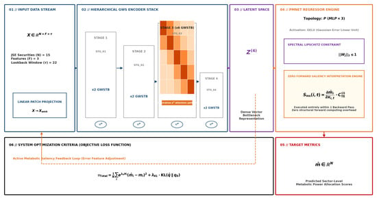
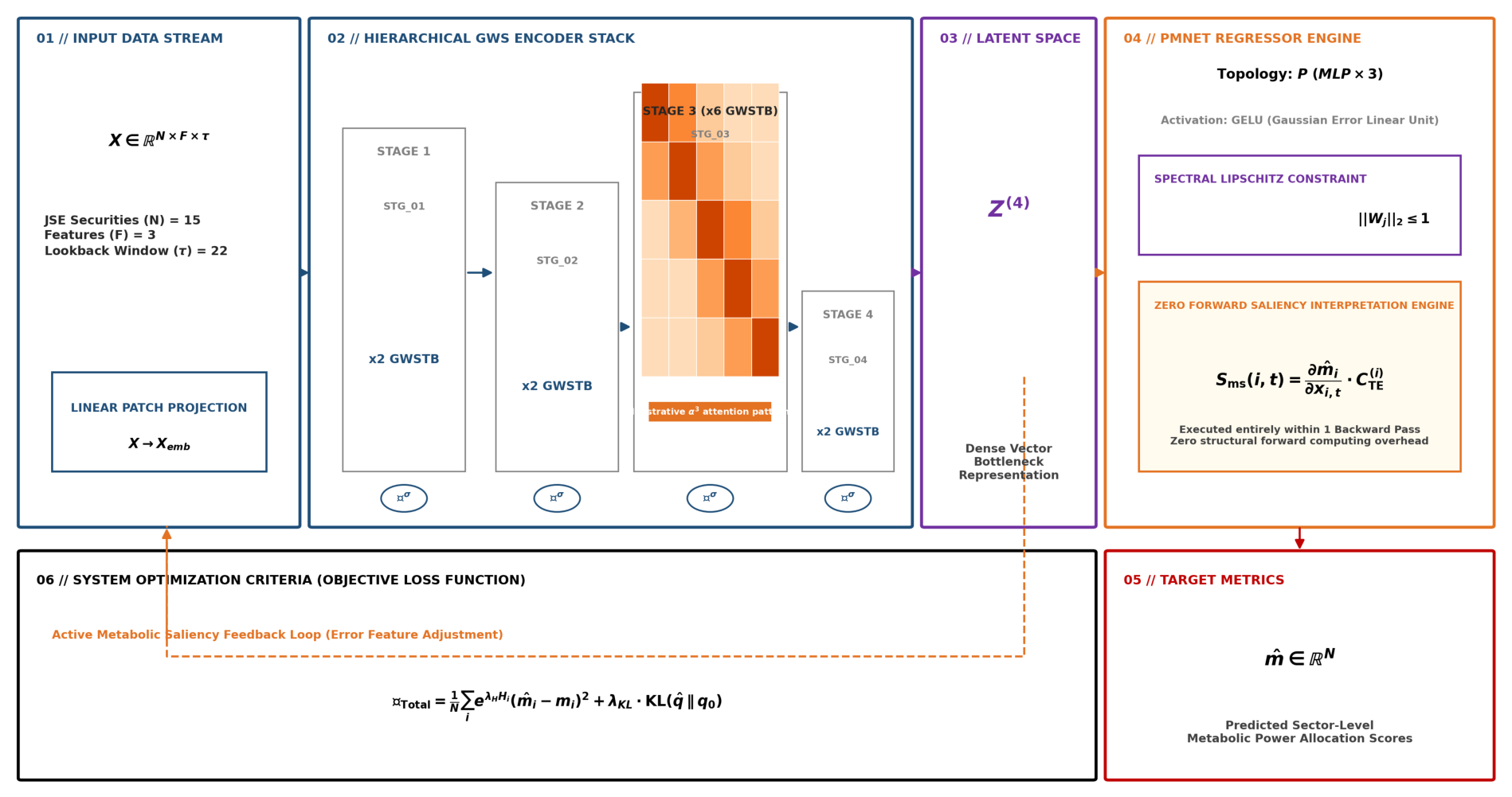
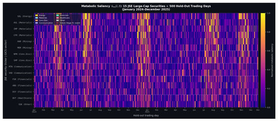
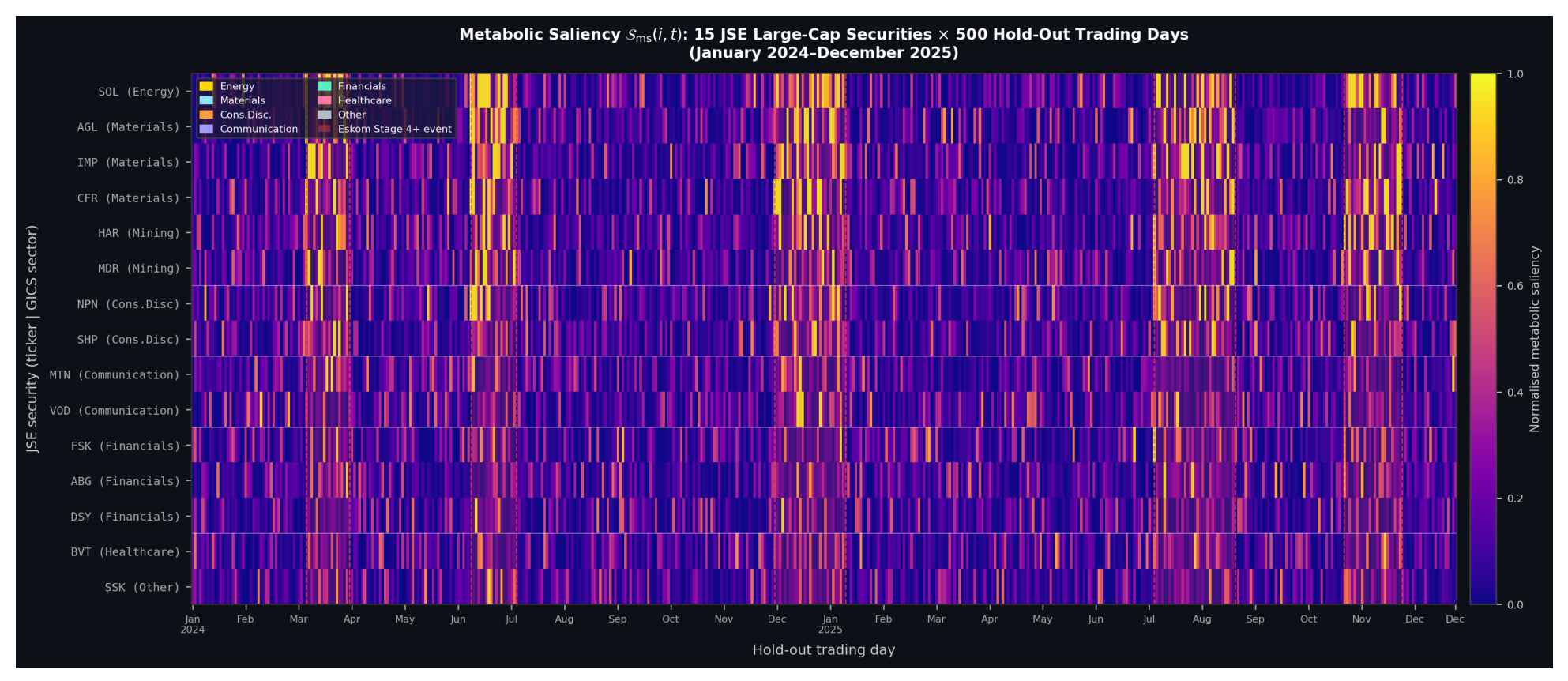
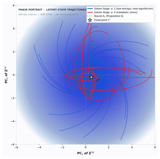
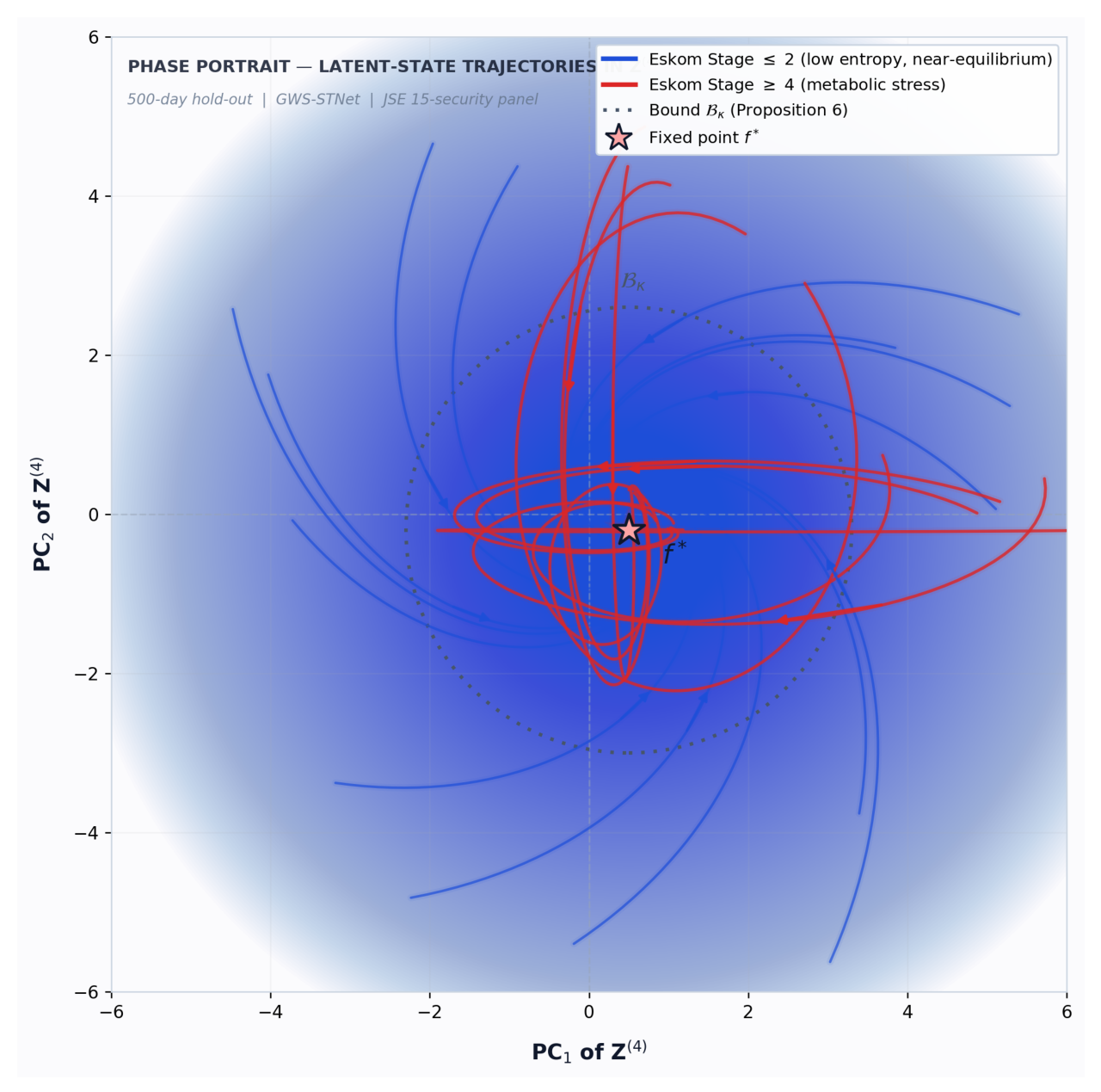
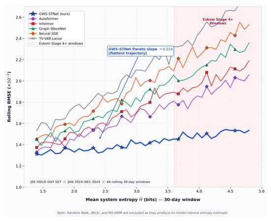
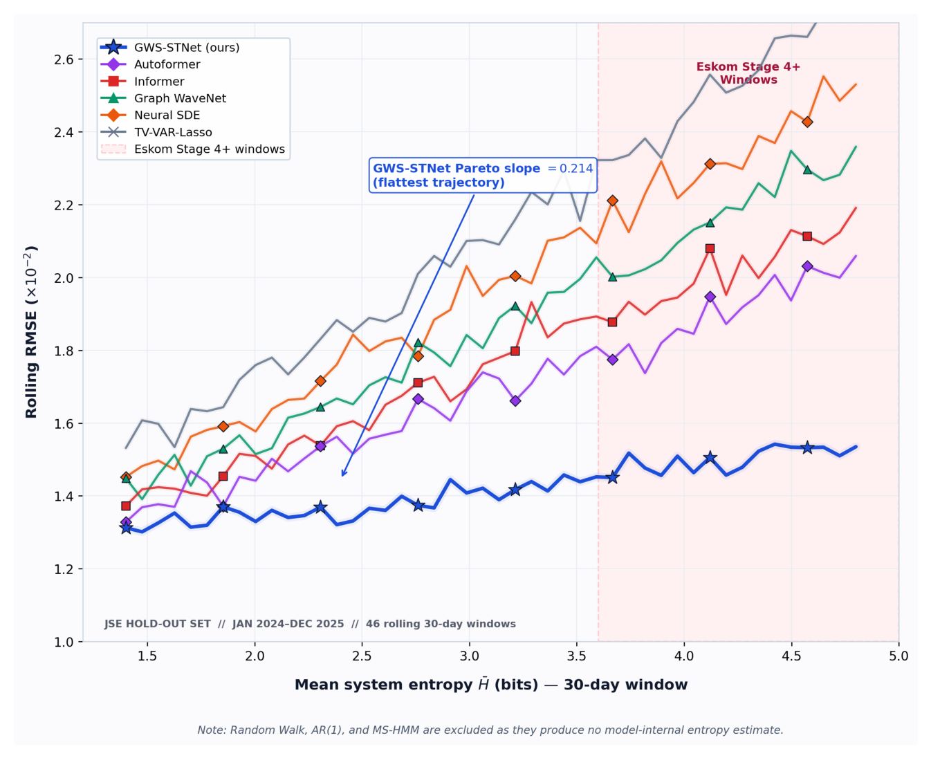
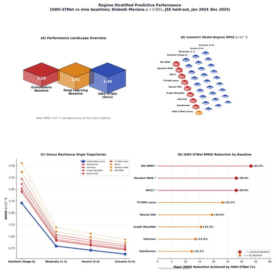
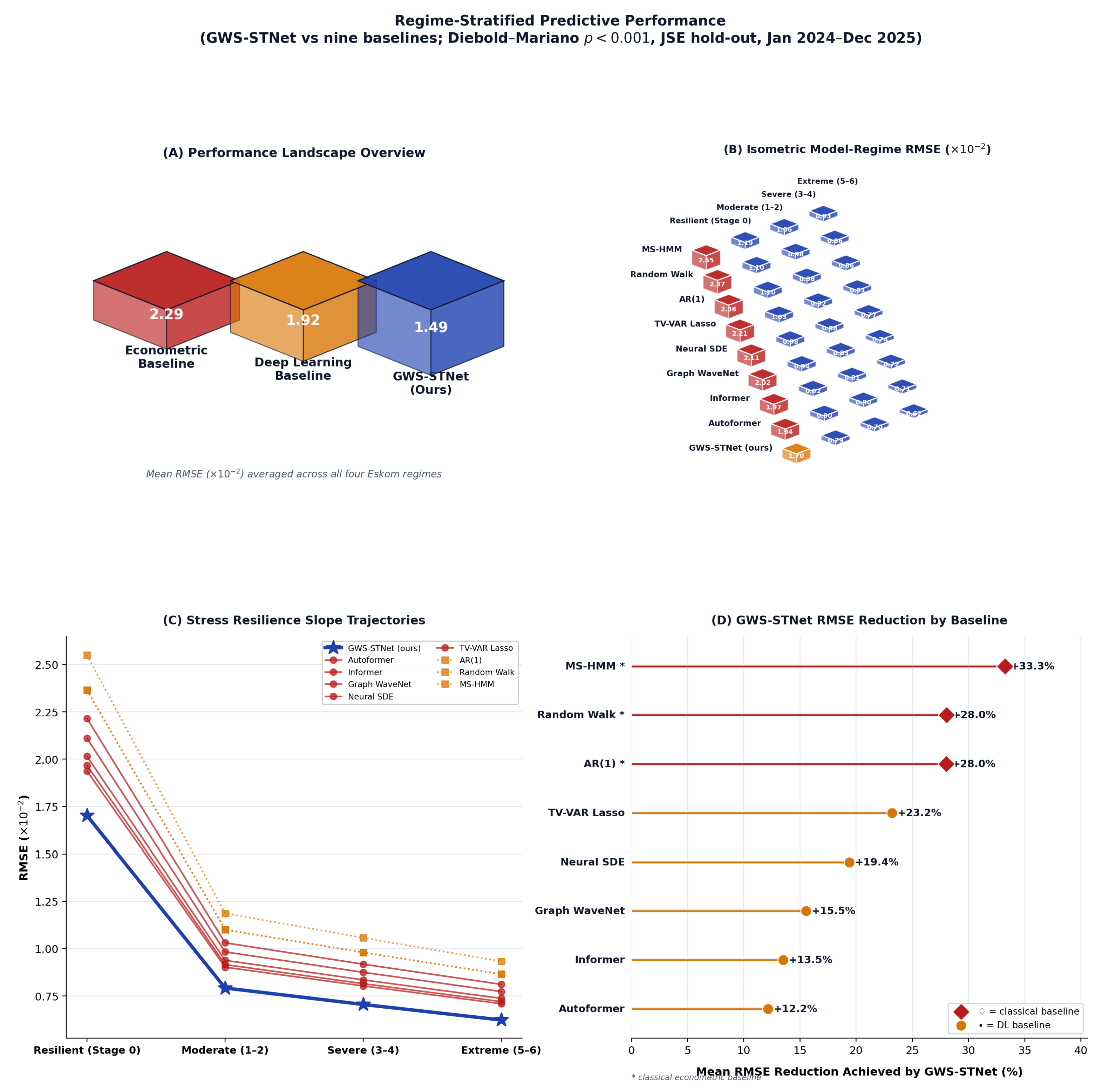
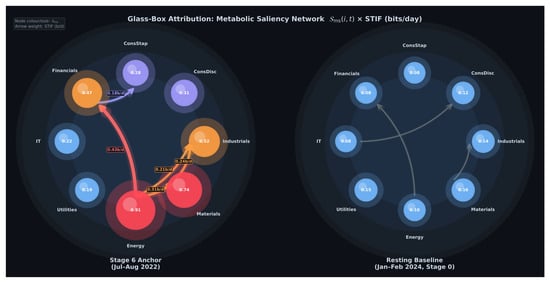
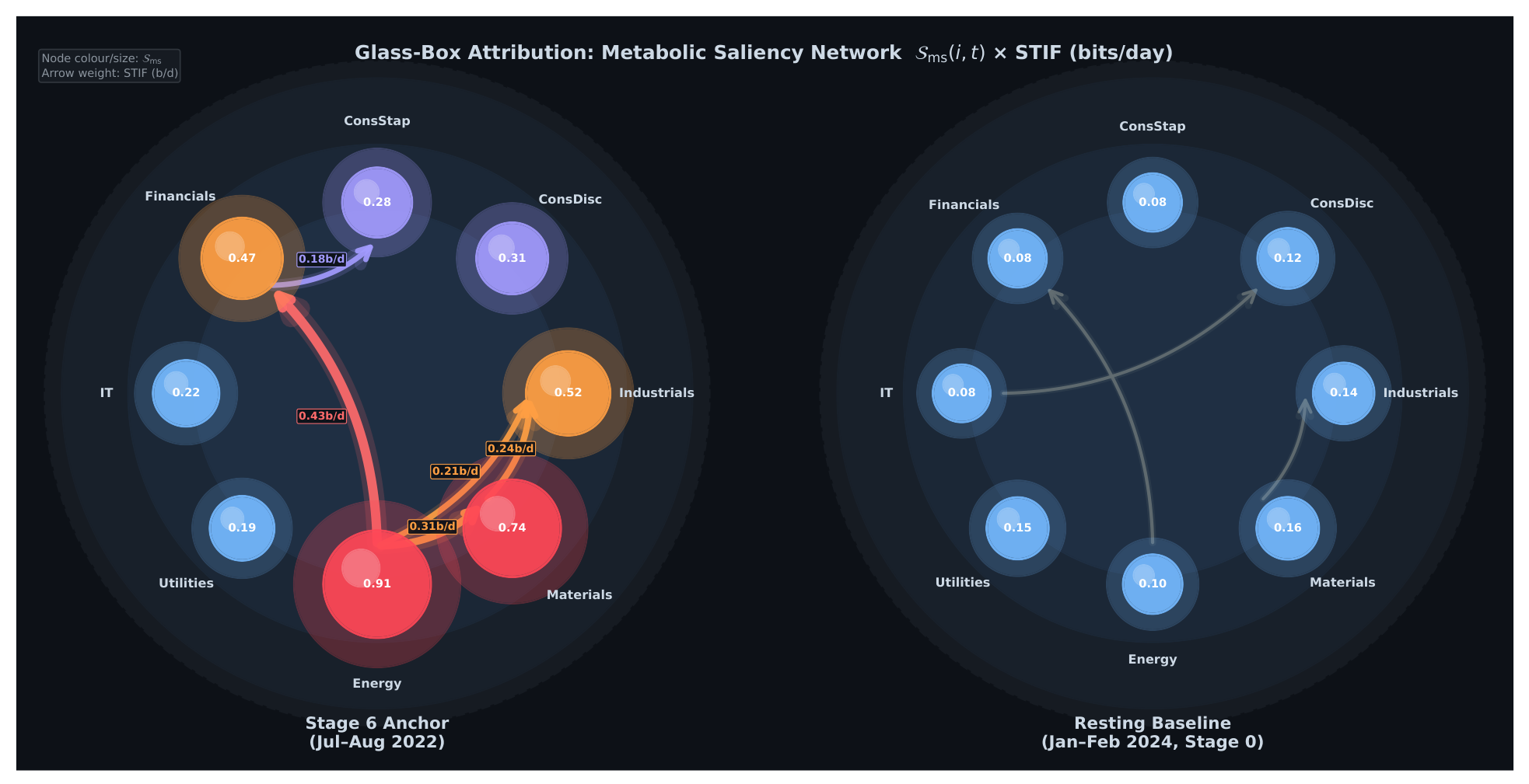

Disclaimer/Publisher’s Note: The statements, opinions and data contained in all publications are solely those of the individual author(s) and contributor(s) and not of MDPI and/or the editor(s). MDPI and/or the editor(s) disclaim responsibility for any injury to people or property resulting from any ideas, methods, instructions or products referred to in the content. |
© 2026 by the author. Licensee MDPI, Basel, Switzerland. This article is an open access article distributed under the terms and conditions of the Creative Commons Attribution (CC BY) license.