A Regularized Numerical Solution to an Inverse Coefficient Problem for the Forced Vibrations of a Cantilever Beam Equation Under Nonlocal Conditions

Abstract

This study tackles a fourth-order inverse problem involving a cantilever beam with nonlocal conditions to simultaneously calculate the beam’s displacement and an unknown time-dependent coefficient. A finite difference approach is suggested to discretize the hyperbolic fourth-order equation. A stability analysis for the proposed scheme is also provided. The indirect problem is the minimization of the misfit function. The goal of the minimization algorithm is to reduce the gap between the measured (noisy) data and the numerical computed solution provided by the model. To achieve stable results, Tikhonov’s regularization technique is employed, and two numerical test examples are shown to illustrate the suggested scheme’s reliability. The unknown potential terms are successfully reconstructed, and stability and accuracy are maintained even in the presence of noise following the application of the Tikhonov regularization method. A trial-and-error strategy and the L-curve method are employed to obtain the optimal value for the regularization parameter.

1. Background

In mathematics, a partial differential equation (PDE) involves a multivariable function and one or more of its partial derivatives. PDEs play a vital role in many science- and knowledge-related applications, linking mathematics to other subjects such as physics, chemistry, biology, etc. In the fields of engineering design, construction and medicine, for example, high-speed computers have greatly influenced the development of numerical methods for solving PDEs, allowing them to be advanced and modernized to a greater extent than other analytical methods. PDE analyses primarily focus on the behavior and characteristics of PDE solutions [1,2,3,4].

A direct problem (DP) is a mathematical or physical problem that involves calculating results or outputs based on specific data or preliminary conditions; in other words, the solution involves predicting the effects based on a complete description of their causes. This concept is used in many fields, such as engineering, physics, and applied mathematics, in which differential equations or other mathematical models are commonly used to describe the relationship between inputs and results [5,6,7].

Inverse problems (IPs) occur in many aspects of human life, including biology, medicine, mineral mining, seismology, and industrial product quality control, which are expressed in modern mathematical problems. Many of the aforementioned applications are modeled with PDEs. It is possible to find solutions to determine the system’s behavior once the values or conditions have been defined [8,9]. Some of the necessary input data include boundary and initial conditions, the geometry of the solution domain, and forcing terms. It will be impossible to determine the behavior of the physical systems based on incomplete input data. Nevertheless, certain outputs can be quantified through experimental methods, and this information can be employed to infer the absent input data alongside the known input data. This is recognized as an IP. However, these are typically ill-posed and exhibit instability. This suggests that even minor modifications to the input data can result in significant variations in the output solution [10,11].

The fundamental theory and analysis of IPs were developed in the foundational works of Tikhonov [12], Ivanov [13], Lavrentiev et al. [14], and others. Additionally, many other authors have examined the hyperbolic equation under the overspecified general integral type condition [15]. Hussein and Lesnic [16] examined the wave inverse problem using the FDM with Tikhonov regularization. Using the separation of variables, in [17], Shilan and other researchers used FDM to solve wave and hyperbolic equations under different conditions. The authors examined an IP to determine an unknown term in fourth-order PDEs, as shown in [18]. In ref. [19,20], the authors investigated IPs aimed at determining unknown coefficients within second-order hyperbolic equations. The authors established a time-domain FDM to simulate bending wave propagation in infinite beams resting on an elastic foundation [21]. In ref. [22,23], approximate methods are proposed for addressing direct and IPs associated with the inhomogeneous Bernoulli–Euler equation that describes beam vibrations. In ref. [24,25], the authors solved an IP that involved reconstructing the time-dependent coefficient in a one-dimensional hyperbolic equation. In ref. [26], Anatoly and Alexander utilized the fast Fourier transform to address the wave equation with integral data. In ref. [27], the anisotropic elastic half-space surface wave propagation problem was solved using the Laplace domain boundary element method. In ref. [28,29], researchers used FDM with the separation-of-variables approach to solve wave and hyperbolic equations under various conditions. Mehraliyev and Huseynova [30] investigated the solvability of the IP associated with the fourth-order pseudo-hyperbolic equation, incorporating an uncertain time-dependent coefficient. In reference [31], the conditions for unique solvability for the inverse problem solution were given for the fourth-order hyperbolic equation in order to determine the lowest term coefficient.

Recently, this research area has attracted specific attention regarding a fourth-order linear differential equation. It describes the transverse vibrations of a homogeneous beam influenced by an external force and excludes rotational motion during bending [32,33]. In Ref. [34], the researchers established the existence and uniqueness of the fourth order of the inverse boundary value problem.

In this paper, we present a numerical method to solve the fourth-order IP associated with the equation of forced vibrations of a cantilever beam subject to integral type conditions and the Neumann condition, as described in Section 2. Section 3 presents the investigated IPs discretized using the FDM to solve the (nonlocal) direct problem. An iterative optimization algorithm based on the trust-region-reflective method encoded within the lsqnonlin routine in MATLAB’s optimization toolbox [35] is employed to address the IP and described in Section 4. The algorithm aims to reduce the discrepancy between the model-generated result and the observed data. We employ Tikhonov’s regularization methods to stabilize the solution of the IP. The numerical findings and reconstructions of unknown coefficients are discussed in Section 5. Finally, the conclusions and suggestions for future work are outlined in Section 6.

2. Mathematical Setting of IP

Let $D_T$ ≔ {0 < $\chi$ < 1, 0 < $\tau$ < T} be a rectangular domain. We examine the following IP: identify a pair of functions $\left(\mathcal{w}\right(\chi , \tau ), a( \tau \left)\right)$ that fulfill the one-dimensional forced vibration equation for a cantilever beam.

$${\mathcal{w}}_{ \tau \tau }\left(\chi , \tau \right)+{\alpha \mathcal{w}}_{\chi \chi \chi \chi }\left(\chi , \tau \right)=a\left( \tau \right)\mathcal{w}\left(\chi , \tau \right)+G\left(\chi , \tau \right)$$

(1)

under the assumption of nonlocal initial conditions,

$$\begin{gathered} \mathcal{w}(\chi ,0)=\varphi \left(\chi \right)+I_1\left(\chi \right), 0 \le \chi \le 1, \\ {\mathcal{w}}_{ \tau }\left(\chi ,0\right)=\psi \left(\chi \right)+I_2\left(\chi \right), 0 \le \chi \le 1, \end{gathered}$$

(2)

where $I_{\mathcal{o}}\left(\chi \right)={\int }_0^T{\rho }_{\mathcal{o}}\left(\tau \right)u\left(\chi ,\tau \right)d\tau , for \mathcal{o}=\mathrm{1,2}.$

Neumann boundary conditions

$${\mathcal{w}}_{\chi }\left(0, \tau \right)={\mathcal{w}}_{\chi }\left(1, \tau \right)={\mathcal{w}}_{\chi \chi \chi }\left(0, \tau \right)=0, 0\le \tau \le T,$$

(3)

with nonlocal integral conditions

$${\int }_0^1\mathcal{w}\left(\chi ,\tau \right)d\chi =0, 0\le \tau \le T,$$

(4)

and the extra data condition is given by

$$\mathcal{w}\left(0, \tau \right)=h\left( \tau \right), 0\le \tau \le T,$$

(5)

where $\alpha$ > 0 is a known number and is related to some of the physical properties of the beam, such as the Young’s modulus and moment of inertia [34].

Equations (1)–(5) are called IPs. $G,\varphi ,\psi ,{\rho }_{\mathfrak{i}}\left( \tau \right), \left(\mathfrak{i}=\mathrm{1,2}\right)$ and ℎ ($\tau$) are the provided functions. In physical applications, the term represents various phenomena. It might be considered as a force or damping/amplifying force change with time. $\mathcal{w}$ ($\chi$, $\tau$) represent the wave transverse displacement of the beam at a specific position along its length and at a specific time. The unique solvability of the aforementioned IP was investigated in [34].

In standard direct problems, classical local initial conditions (as described in (2)) are sufficient for a well-posed system. However, in the scope of inverse problems (IPs) where source terms or coefficients like $a\left(\tau \right)$ are unknown, classical initial conditions can lead to ill-posedness or fail to guarantee a unique solvability of the IP. The nonlocal initial conditions, which incorporate the integral terms $I_1\left(\chi \right)$ and $I_2\left(\chi \right)$ over the specific time interval, provide a regularization/stabilization effect. They link the initial state to the temporal evolution of the system, ensuring better stability and uniqueness when recovering the unknown time-dependent parameter $a\left(\tau \right)$ [4].

Physically, these conditions describe systems exhibiting “memory effects” or closed-loop feedback mechanisms. For a cantilever beam, especially in smart structures (e.g., those equipped with piezoelectric sensors and actuators), the initial displacement and velocity are not merely independent static states. Instead, they are influenced by a feedback control system that monitors the beam’s vibration over the time period $T$. The integrals $I_1\left(\chi \right)$ and $I_2\left(\chi \right)$ represent time-averaged observations. This models scenarios where precise instantaneous initial measurements are impossible due to sensor latency, and the initial state must instead be inferred from time-averaged sensor data weighted by the kernels ${\rho }_1\left(\tau \right)$ and ${\rho }_2\left(\tau \right)$.

Condition (4) ensures that the net spatial average of the beam’s transverse displacement is zero at any given time $\tau$. Physically, this represents a structural or environmental constraint in which the area displaced in the positive direction is exactly equal to the area displaced in the negative direction [33].

Definition 1.

The classical solution to the inverse boundary value problem (1)–(5) involves the pair { $\mathcal{w}$($\chi$, $\tau$), $a\left(\tau \right)$} and the function $\mathcal{w}$($\chi$, $\tau$)$\in {\overline{C}}^{\mathrm{4,2}}\left(D_T\right)$ and $a\left(\tau \right)\in C[0,T]$ that satisfy equation (1) in $D_T$, condition (2) in [0,1], and conditions (3)–(5) in $[0,T]$, where

$${\overline{C}}^{\mathrm{4,2}}\left(D_T\right)=\left\{\mathcal{w}\left(\chi , \tau \right):\mathcal{w}\left(\chi , \tau \right)\in C^2\left(D_T\right) ,{\mathcal{w}}_{\chi \chi \chi \chi }\left(\chi , \tau \right)\in C\left(D_T\right)\right\}.$$

Theorem 1.

Assume that $G(\chi , \tau )\in C\left({\bar{D}}_T\right),\phi \left(\chi \right),\psi \left(\chi \right)\in C\left[\mathrm{0,1}\right],{\rho }_{\mathfrak{i}}( \tau )\in C[0,T],$ $\left(\mathfrak{i}=\mathrm{1,2}\right),h\left( \tau \right)\in C^2\left[0,T\right], h\left(\tau \right)\ne 0, {\int }_0^1 G\left(\chi , \tau \right)d\chi =0$ for $\left(0\le \tau \le T\right)$, and the compatibility conditions

$${\int }_0^1 \phi (\chi )d\chi =0, {\int }_0^1 \psi (\chi )d\chi =0,$$

(6)

$$\phi (0)+{\int }_0^T {\rho }_1(\tau )h(\tau )d\tau =h(0), \psi (0)+{\int }_0^T {\rho }_2(\tau )h(\tau )d \tau =h^{\prime }(0),$$

(7)

hold. Then the following assertions are valid:

• Each classical solution $\left\{\mathcal{w}\right(\chi , \tau ),a(\tau \left)\right\}$ to problems (1)–(5) is a solution to problems (1)–(3), (6), and (7).
• Each solution $\left\{\mathcal{w}\right(\chi , \tau ),a(\tau \left)\right\}$ to the problem (1)–(3), (6), (7) is a classical solution to problems (1)–(5). If

  $$\left(T{‖{\rho }_2\left(\tau \right)‖}_{C[0,T]}+{‖{\rho }_1\left(\tau \right)‖}_{C[0,T]}+\frac{T}{2}{\Vert a\left(\tau \right)\Vert }_{C[0,T]}\right) T<1$$

  (8)

Theorem 2.

Let us assume that the data of inverse problem (1)–(3) and (6)–(7) satisfy the following conditions:

• $\phi \left(\chi \right)\in C^4\left[\mathrm{0,1}\right],{\phi }^{‴}\left(\chi \right)\in L_2\left(\mathrm{0,1}\right)$ and ${\phi }^{\prime }\left(0\right)={\phi }^{\prime }\left(1\right)={\phi }^{‴}\left(0\right)={\phi }^{‴}\left(1\right)=0$.
• $\psi \left(\chi \right)\in C^2\left[\mathrm{0,1}\right],{\psi }^{″}\left(\chi \right)\in L_2\left(\mathrm{0,1}\right)$ and ${\psi }^{\prime }\left(0\right)={\psi }^{\prime }\left(1\right)=0$.
• $G(\chi ,\tau ),G_{\chi }(\chi ,\tau ),G_{\chi \chi }(\chi ,\tau )\in C\left({\bar{D}}_T\right),G_{\chi \chi \chi }(\chi ,\tau )\in L_2\left(D_T\right)$, $G_{\chi }(0,\tau )=G_{\chi }(1,\tau )=0,(0\le \tau \le T)$.
• $\alpha >0,{\rho }_{\mathfrak{i}}\left(\tau \right)\in C[0,T](\mathfrak{i}=\mathrm{1,2}),h( \tau )\in C^2[0,T],h( \tau )\ne 0,(0\le \tau \le T)$,

and

$$\left(B\right(T\left)\right(A\left(T\right)+2)+C(T\left)\right)\left(A\right(T)+2)<1.$$

and

$$\begin{array}{c}{\int }_0^1 G(\chi , \tau )d\chi =0, (0\le \tau \le T), {\int }_0^1 \phi \left(\chi \right)d\chi =0, {\int }_0^1 \psi \left(\chi \right)d\chi =0\\ \phi \left(0\right)+{\int }_0^T {\rho }_1\left(\tau \right)h\left(\tau \right)d\tau =h\left(0\right), \psi \left(0\right)+{\int }_0^T {\rho }_2\left(\tau \right)h\left(\tau \right)d\tau =h^{\prime }\left(0\right)\end{array}$$

Then, the problem (1)–(7) has a unique classical solution in the ball $K=K_R\left(\Vert z{\Vert }_{E_T^5}\le R\le A\left(T\right)+2\right)$ of the space $E_T^5$ only, where

$$\begin{gathered} A\left(T\right)=A_1\left(T\right)+A_2\left(T\right), \\ B\left(T\right)=B_1\left(T\right)+B_2\left(T\right), \\ C\left(T\right)=C_1\left(T\right)+C_2\left(T\right), \\ {A}_1\left(T\right)=\Vert \phi (\chi ){\Vert }_{L_2(\mathrm{0,1})}+T\Vert \psi (\chi ){\Vert }_{L_2(\mathrm{0,1})}+T\sqrt{T}\Vert G(\chi , \tau ){\Vert }_{L_2\left(D_T\right)}+\sqrt{6}{‖{\phi }^{(5)}(\chi )‖}_{L_2(\mathrm{0,1})}+\sqrt{{\displaystyle \frac{6}{\alpha }}}{‖{\psi }^{(3)}(\chi )‖}_{L_2(\mathrm{0,1})}+\sqrt{{\displaystyle \frac{6}{\alpha }}T}{‖G_{\chi \chi \chi }(\chi , \tau )‖}_{L_2\left(D_T\right)}, \\ {B}_1\left(T\right)=\left(T+\sqrt{{\displaystyle \frac{6}{\alpha }}}\right)T, \\ {C}_1(T)=T(1+\sqrt{6}){‖{\rho }_1(\tau )‖}_{C[0,T]}+T\left(T+\sqrt{{\displaystyle \frac{6}{\alpha }}}\right){‖{\rho }_2(\tau )‖}_{C[0,T]}, \\ {A}_2\left(T\right)={‖[h(\tau ){]}^{-1}‖}_{C[0,T]}\{{‖h^{″}( \tau )-G(0, \tau )‖}_{C[0,T]}+{\left({\displaystyle {\sum }_{k=1}^{\mathrm{\infty }}} {\lambda }_k^{-2}\right)}^{{\displaystyle \frac{1}{2}}}\left[\alpha {‖{\phi }^{(5)}(\chi )‖}_{L_2(\mathrm{0,1})}+\sqrt{\alpha }{‖{\psi }^{(3)}(\chi )‖}_{L_2(\mathrm{0,1})}+\sqrt{\alpha T}{‖G_{\chi \chi \chi }(\chi , \tau )‖}_{L_2\left(D_T\right)}\right]\}, \\ {B}_2(T)={‖[h( \tau ){]}^{-1}‖}_{C[0,T]}{\left({\displaystyle {\sum }_{k=1}^{\mathrm{\infty }}} {\lambda }_k^{-2}\right)}^{{\displaystyle \frac{1}{2}}}\sqrt{\alpha }T, \\ {C}_2(T)={‖[h( \tau ){]}^{-1}‖}_{C[0,T]}{\left({\displaystyle \sum _{k=1}^{\mathrm{\infty }}} {\lambda }_k^{-2}\right)}^{{\displaystyle \frac{1}{2}}}T\left(\alpha {‖{\rho }_1(\tau )‖}_{C[0,T]}+\sqrt{\alpha }{‖{\rho }_2(\tau )‖}_{C[0,T]}\right). \end{gathered}$$

Proof. 

See [34]. □

3. Discretization of the DP (1)–(4)

Consider that the direct (forward) problem includes the governing equations (1)–(4) and the desired output data (5). The only unknown quantity in this DP that needs to be determined is $\mathcal{w}(\chi , \tau )$, while all remaining quantities are provided. Equation (1) is discretized using the following FDM form: choose two positive integer numbers $M,N>0$ and define $\Delta \chi ={\displaystyle \frac{1}{M}}$, $\Delta \tau ={\displaystyle \frac{T}{N}}$. Also denote the $\mathcal{w}\left({\chi }_{\mathfrak{i}},{ \tau }_n\right)={\mathcal{w}}_{\mathfrak{i},n}$, $G\left({\chi }_{\mathfrak{i}},{ \tau }_n\right)=G_{\mathfrak{i},n}$, ${\mathsf{\varphi }}_{\mathfrak{i}}=\mathsf{\varphi }\left({\chi }_{\mathfrak{i}}\right)$, ${\psi }_{\mathfrak{i}}=\psi \left({\chi }_{\mathfrak{i}}\right),$ where the space node is ${\chi }_{\mathfrak{i}}=\mathfrak{i}\Delta \chi$, and time node ${\tau }_n=n\Delta \tau ,\mathfrak{i}=\mathrm{0,1},\dots ,M,n=\mathrm{0,1},2,\dots ,N.$ Utilizing Crank–Nicolson FDM [36], Equation (1) is discretized as follows:

$$\begin{array}{l}{\displaystyle \frac{{\mathcal{w}}_{\mathfrak{i},n+1}-2{\mathcal{w}}_{\mathfrak{i},n}+{\mathcal{w}}_{\mathfrak{i},n-1}}{{(∆ \tau )}^2}}\\ =-\alpha ({\displaystyle \frac{{\mathcal{w}}_{\mathfrak{i}+2,n+1}-4{\mathcal{w}}_{\mathfrak{i}+1,n+1}+6{\mathcal{w}}_{\mathfrak{i},n+1}-{4 \mathcal{w}}_{\mathfrak{i}-1,\mathfrak{i}n+1}+{\mathcal{w}}_{\mathfrak{i}-2,n+1}}{2{\left(∆\chi \right)}^4}}\\ + {\displaystyle \frac{{\mathcal{w}}_{\mathfrak{i}+2,n}-4{\mathcal{w}}_{\mathfrak{i}+1,n}+6{\mathcal{w}}_{\mathfrak{i},n}-{4 \mathcal{w}}_{\mathfrak{i}-1,n}+{\mathcal{w}}_{\mathfrak{i}-2,n}}{2{\left(∆\chi \right)}^4}})+{\displaystyle \frac{1}{2}}[a_n{\mathcal{w}}_{\mathfrak{i},n}+G_{\mathfrak{i},n}+a_{n+1}{\mathcal{w}}_{\mathfrak{i},n+1}\\ +G_{\mathfrak{i},n+1}]\end{array}$$

(9)

$$\mathcal{w}\left({\chi }_{\mathfrak{i}},0\right)=\mathsf{\varphi }\left({\chi }_{\mathfrak{i}}\right)+I_1\left({\chi }_{\mathfrak{i}}\right)$$

(10)

$${\mathcal{w}}_{\tau }\left({\chi }_{\mathfrak{i}},0\right)={\displaystyle \frac{{\mathcal{w}}_{\mathfrak{i},1}-{\mathcal{w}}_{\mathfrak{i},-1}}{2\Delta \tau }}=\psi \left({\chi }_{\mathfrak{i}}\right)+I_2({\chi }_{\mathfrak{i}})$$

(11)

$${\mathcal{w}}_{\chi }\left(0,t_n\right)={\displaystyle \frac{{\mathcal{w}}_{1,n}-{\mathcal{w}}_{-1,n}}{2∆x}}=0$$

(12)

$${\mathcal{w}}_{\chi }\left(1,t_n\right)={\displaystyle \frac{{\mathcal{w}}_{M+1,n}-{\mathcal{w}}_{M-1,n}}{2∆\chi }}=0$$

(13)

$$\begin{gathered} {\mathcal{w}}_{\chi \chi \chi }\left(0,t_n\right)={\displaystyle \frac{{\mathcal{w}}_{2,n}-2{\mathcal{w}}_{1,n}+2{\mathcal{w}}_{-1,n}-{\mathcal{w}}_{-2,n}}{2{(∆\chi )}^3}}=0, \\ \mathrm{for} \mathfrak{i}=\mathrm{0,1},\dots .,M. n=\mathrm{0,1},\dots .,N. \end{gathered}$$

(14)

Furthermore, the integral condition described in (4) is approximated using the trapezoidal rule, yielding the following discrete form:

$$\begin{array}{l}{\displaystyle \frac{∆\chi }{2}}\left[{\mathcal{w}}_{0n}+{\mathcal{w}}_{Mn}+2{\displaystyle \sum _{\mathfrak{i}=1}^{M-1}} {\mathcal{w}}_{\mathfrak{i}n}\right]=0,\\ n=\mathrm{0,1},\dots ,N,\end{array}$$

(15)

Also, the integrals in (7) and (8) are approximated as

$$I_1\left({\chi }_i\right)={\displaystyle \frac{∆ \tau }{2}}\left\{{\rho }_1\left({\tau }_0\right){\mathcal{w}}_{\mathfrak{i}0}+{\rho }_1\left({\tau }_N\right){\mathcal{w}}_{\mathfrak{i}N}+2{\displaystyle \sum _{n=1}^{N-1}}{\rho }_1\left({\tau }_n\right){\mathcal{w}}_{\mathfrak{i}\mathrm{n}}\right\},$$

and

$$\begin{gathered} I_2\left({\chi }_i\right)={\displaystyle \frac{∆ \tau }{2}}\left\{{\rho }_2\left({ \tau }_0\right){\mathcal{w}}_{\mathfrak{i}0}+{\rho }_2\left({ \tau }_N\right){\mathcal{w}}_{\mathfrak{i}N}+2{\displaystyle \sum _{n=1}^{N-1}}{\rho }_2\left({ \tau }_n\right){\mathcal{w}}_{\mathfrak{i}\mathrm{n}}\right\}, \\ \mathrm{for}\mathfrak{i}=\mathrm{0,1},\dots .,M. \end{gathered}$$

Equation (9) can be regrouped in a difference equation of the form

$$\begin{array}{l}{\displaystyle \frac{\zeta }{2}}{\mathcal{w}}_{\mathfrak{i}-2,n+1}-2\zeta {\mathcal{w}}_{\mathfrak{i}-1,n+1}+\left(1+A_{n+1}\right){\mathcal{w}}_{\mathfrak{i},n+1}-2\zeta {\mathcal{w}}_{\mathfrak{i}+1,n+1}+{\displaystyle \frac{\zeta }{2}}{\mathcal{w}}_{\mathfrak{i}+2,n+1 }\\ =-{\displaystyle \frac{\zeta }{2}}{\mathcal{w}}_{\mathfrak{i}-2,n}+2\zeta {\mathcal{w}}_{\mathfrak{i}-1,n}+\left(2-A_n\right){\mathcal{w}}_{\mathfrak{i},n}+2\zeta {\mathcal{w}}_{\mathfrak{i}+1,n}\\ -{\displaystyle \frac{\zeta }{2}}{\mathcal{w}}_{\mathfrak{i}+2,n}{-\mathcal{w}}_{\mathfrak{i},n-1}+{\displaystyle \frac{{(∆ \tau )}^2}{2}}\left[G_{\mathfrak{i},n+1}+G_{\mathfrak{i},n}\right] ,\end{array}$$

(16)

where

$$\zeta ={\displaystyle \frac{\alpha (∆{ \tau )}^2}{{\left(∆\chi \right)}^4}}, A_n={\displaystyle \frac{3\alpha {(∆ \tau )}^2}{{\left(∆\chi \right)}^4}}-{\displaystyle \frac{{(∆ \tau )}^2}{2}}{a}_n,$$

since the FDM scheme is two-time layer, we need to elaborate on the initial and boundary conditions in order to handle some points located outside the computational domain, as we will explain below.

For $\mathfrak{i}=0$ and $n=0$, using conditions (11), (12), and (14) in Equation (16) will take the following form:

$$\begin{array}{l}\left(2+A_1\right){\mathcal{w}}_{\mathrm{0,1}}-4\zeta {\mathcal{w}}_{\mathrm{1,1}}+{\zeta \mathcal{w}}_{\mathrm{2,1} }\\ =\left(2-A_0\right){\mathcal{w}}_{\mathrm{0,0}}+4\zeta {\mathcal{w}}_{\mathrm{1,0}}-{\zeta \mathcal{w}}_{\mathrm{2,0}}+{\displaystyle \frac{{(∆ \tau )}^2}{2}}\left[G_{\mathrm{0,1}}+ G_{\mathrm{0,0}}\right]+2\Delta \tau \psi \left({\chi }_0\right)\\ +2\Delta \tau I_2\left({\chi }_0\right).\end{array}$$

(17)

For $\mathfrak{i}=M-1 \mathrm{a}\mathrm{n}\mathrm{d} n=0,$ using condition (14) in Equation (16), we have

$$\begin{array}{l}{\displaystyle \frac{\zeta }{2}}{\mathcal{w}}_{M-\mathrm{3,1}}-2\zeta {\mathcal{w}}_{M-\mathrm{2,1}}+\left(2+A_1+{\displaystyle \frac{\zeta }{2}}\right){\mathcal{w}}_{M-\mathrm{1,1}}-2\zeta {\mathcal{w}}_{M,1}\\ =-{\displaystyle \frac{\zeta }{2}}{\mathcal{w}}_{M-\mathrm{3,0}}+2\zeta {\mathcal{w}}_{M-\mathrm{2,0}}+\left(2-A_0-{\displaystyle \frac{\zeta }{2}}\right){\mathcal{w}}_{M-\mathrm{1,0}}+2\zeta {\mathcal{w}}_{M,0}\\ +{\displaystyle \frac{∆{ \tau }^2}{2}}\left[G_{M-\mathrm{1,1}}+G_{M-\mathrm{1,0}}\right]+2\Delta \tau \psi \left({\chi }_{M-1}\right)+2\Delta \tau I_2\left({\chi }_{M-1}\right).\end{array}$$

(18)

For $\mathfrak{i}=M \mathrm{a}\mathrm{n}\mathrm{d} n=0$, we use the approximated version of the condition (4) via Formula (15).

A more practical way to express Equations (16)–(18) can be represented in the matrix form

$$\mathit{L}{v}^{\left(1\right)}=\mathit{E}{v}^{\left(0\right)}+\mathrm{Z}.$$

(19)

where $\mathit{L},\mathit{E}$ are matrices given by

$$\mathit{L}={\left(\begin{array}{ccccccc}2+A_1& -4\zeta & \zeta & 0& \dots & 0& 0\\ -2\zeta & 2+{\displaystyle \frac{\zeta }{2}}+A_1& -2\zeta & {\displaystyle \frac{\zeta }{2}}& 0& 0& 0\\ {\displaystyle \frac{\zeta }{2}}& -2\zeta & 2+A_1& -2\zeta & {\displaystyle \frac{\zeta }{2}}& 0& 0\\ 0& {\displaystyle \frac{\zeta }{2}}& -2\zeta & 2+A_1& -2\zeta & {\displaystyle \frac{\zeta }{2}}& 0\\ ⋮& \ddots & \ddots & \ddots & \ddots & \ddots & ⋮\\ 0& 0& {\displaystyle \frac{\zeta }{2}}& -2\zeta & 2+A_1& -2\zeta & {\displaystyle \frac{\zeta }{2}}\\ ⋮& ⋮& ⋮& ⋮& ⋮& ⋮& ⋮\\ 0& 0& 0& {\displaystyle \frac{\zeta }{2}}& -2\zeta & 2+{\displaystyle \frac{\zeta }{2}}+A_1& -2\zeta \\ 1& 2& 2& 2& 2& 2& 1\end{array}\right)}_{(M+1)\times (M+1)},$$

$$\mathit{E}={\left(\begin{array}{ccccccc}2-A_0& 4\zeta & -\zeta & 0& \dots & 0& 0\\ 2\zeta & 2-{\displaystyle \frac{\zeta }{2}}-A_0& 2\zeta & -{\displaystyle \frac{\zeta }{2}}& 0& 0& 0\\ -{\displaystyle \frac{\zeta }{2}}& 2\zeta & 2-A_0& 2\zeta & -{\displaystyle \frac{\zeta }{2}}& 0& 0\\ 0& -{\displaystyle \frac{\zeta }{2}}& 2\zeta & 2-A_0& 2\zeta & -{\displaystyle \frac{\zeta }{2}}& 0\\ ⋮& \ddots & \ddots & \ddots & \ddots & \ddots & ⋮\\ 0& 0& -{\displaystyle \frac{\zeta }{2}}& 2\zeta & 2-A_0& 2\zeta & -{\displaystyle \frac{\zeta }{2}}\\ ⋮& ⋮& ⋮& ⋮& ⋮& ⋮& ⋮\\ 0& 0& 0& -{\displaystyle \frac{\zeta }{2}}& 2\zeta & 2-{\displaystyle \frac{\zeta }{2}}-A_0& 2\zeta \\ 0& 0& 0& 0& 0& 0& 0\end{array}\right)}_{(M+1)\times (M+1)},$$

$$Z={\left(\begin{array}{c}2∆ \tau \psi \left({\chi }_0\right)+2\Delta \tau I_2\left({\chi }_0\right)+{\displaystyle \frac{{(∆ \tau )}^2}{2}}\left[G_{\mathrm{0,1}}+G_{\mathrm{0,0}}\right] \\ 2∆ \tau \psi \left({\chi }_1\right)+{\displaystyle \frac{{(∆ \tau )}^2}{2}}\left[G_{\mathrm{1,1}}+G_{\mathrm{1,0}}\right]\\ ⋮\\ 2∆ \tau \psi \left({\chi }_{M-2}\right)+{\displaystyle \frac{{(∆ \tau )}^2}{2}}\left[G_{M-\mathrm{2,1}}+G_{M-\mathrm{2,0}}\right]\\ 2∆ \tau \psi \left({\chi }_{M-1}\right)+2\Delta \tau I_2\left({\chi }_{M-1}\right)+{\displaystyle \frac{{(∆ \tau )}^2}{2}}\left[G_{M-\mathrm{1,1}}+G_{M-\mathrm{1,0}}\right]\\ 0\end{array}\right)}_{(M+1)\times 1},$$

where $v^0=\left({\mathcal{w}}_{\mathrm{0,0}},{\mathcal{w}}_{\mathrm{1,0}},\dots .,{\mathcal{w}}_{M,0}\right),v^1=\left({\mathcal{w}}_{\mathrm{0,1}},{\mathcal{w}}_{\mathrm{1,1}},\dots ,{\mathcal{w}}_{M,1}\right).$

In the same manner, for the rest of time, $\mathfrak{i}=0$ and is substituted for $n=\mathrm{1,2},\dots .,N$, so in (16) we have the following equation:

$$\begin{array}{l}\left(1+A_2\right){\mathcal{w}}_{0,n+1}-4\zeta {\mathcal{w}}_{1,n+1}+{\zeta \mathcal{w}}_{2,n+1}\\ =\left(2-A_1\right){\mathcal{w}}_{0,n}+4\zeta {\mathcal{w}}_{1,n}-{\zeta \mathcal{w}}_{2,n} +{\displaystyle \frac{{(∆ \tau )}^2}{2}}\left[G_{0,n+1}+ G_{0,n}\right]\\ -{\mathcal{w}}_{0,n-1}.\end{array}$$

(20)

Also, for $\mathfrak{i}=M-1$, we have

$$\begin{array}{l}{\displaystyle \frac{\zeta }{2}}{\mathcal{w}}_{M-3,n+1}-2\zeta {\mathcal{w}}_{M-2,n+1}+\left(1+A_2\right){\mathcal{w}}_{M-1,n+1}-2\zeta {\mathcal{w}}_{M,n+1}+{\displaystyle \frac{\zeta }{2}}{\mathcal{w}}_{M+1,n+1}\\ =-{\displaystyle \frac{\zeta }{2}}{\mathcal{w}}_{M-3,n}+2\zeta {\mathcal{w}}_{M-2,n}+\left(2-A_1\right){\mathcal{w}}_{M-1,n}+2\zeta {\mathcal{w}}_{M,n}-{\displaystyle \frac{\zeta }{2}}{\mathcal{w}}_{M+1,n}\\ +{\displaystyle \frac{{(∆ \tau )}^2}{2}}\left[G_{M-1,n+1}+G_{M-1,n}\right]-{\mathcal{w}}_{M-1,n-1}.\end{array}$$

(21)

Finally, Equations (17) and (18) can be expressed in the following linear algebraic system:

$${\mathit{L}}_1{v}^{(n+1)}={\mathit{L}}_2{v}^{\left(n\right)}+{\mathrm{Z}}_1+U^{(n-1)}.$$

(22)

$${\mathit{L}}_1={\left(\begin{array}{ccccccc}1+A_{n+1}& -4\zeta & \zeta & 0& \dots & 0& 0\\ -2\zeta & 1+{\displaystyle \frac{\zeta }{2}}+A_{n+1}& -2\zeta & {\displaystyle \frac{\zeta }{2}}& 0& 0& 0\\ {\displaystyle \frac{\zeta }{2}}& -2\zeta & 1+A_{n+1}& -2\zeta & {\displaystyle \frac{\zeta }{2}}& 0& 0\\ 0& {\displaystyle \frac{\zeta }{2}}& -2\zeta & 1+A_{n+1}& -2\zeta & {\displaystyle \frac{\zeta }{2}}& 0\\ ⋮& \ddots & \ddots & \ddots & \ddots & \ddots & ⋮\\ 0& 0& {\displaystyle \frac{\zeta }{2}}& -2\zeta & 1+A_{n+1}& -2\zeta & {\displaystyle \frac{\zeta }{2}}\\ ⋮& ⋮& ⋮& ⋮& ⋮& ⋮& ⋮\\ 0& 0& 0& {\displaystyle \frac{\zeta }{2}}& -2\zeta & 1+{\displaystyle \frac{\zeta }{2}}+A_{n+1}& -2\zeta \\ 1& 2& 2& 2& 2& 2& 1\end{array}\right)}_{(M+1)\times (M+1)}$$

$${\mathit{L}}_2={\left(\begin{array}{ccccccc}2-A_n& 4\zeta & -\zeta & 0& \dots & 0& 0\\ 2\zeta & 2-{\displaystyle \frac{\zeta }{2}}-A_n& 2\zeta & -{\displaystyle \frac{\zeta }{2}}& 0& 0& 0\\ -{\displaystyle \frac{\zeta }{2}}& 2\zeta & 2-A_n& 2\zeta & -{\displaystyle \frac{\zeta }{2}}& 0& 0\\ 0& -{\displaystyle \frac{\zeta }{2}}& 2\zeta & 2-A_n& 2\zeta & -{\displaystyle \frac{\zeta }{2}}& 0\\ ⋮& \ddots & \ddots & \ddots & \ddots & \ddots & ⋮\\ 0& 0& -{\displaystyle \frac{\zeta }{2}}& 2\zeta & 2-A_n& 2\zeta & -{\displaystyle \frac{\zeta }{2}}\\ ⋮& ⋮& ⋮& ⋮& ⋮& ⋮& ⋮\\ 0& 0& 0& -{\displaystyle \frac{\zeta }{2}}& 2\zeta & 2-{\displaystyle \frac{\zeta }{2}}-A_n& 2\zeta \\ 0& 0& 0& 0& 0& 0& 0\end{array}\right)}_{(M+1)\times (M+1)},$$

$$U^{(j-1)}={\left(\begin{array}{c}-{\mathcal{w}}_{0,n-1} \\ -{\mathcal{w}}_{1,n-1}\\ ⋮\\ -{\mathcal{w}}_{M-2,n-1}\\ -{\mathcal{w}}_{M-1,n-1}\\ 0\end{array}\right)}_{(M+1)\times 1}, Z_1={\left(\begin{array}{c}{\displaystyle \frac{{(∆ \tau )}^2}{2}}\left[G_{0,n+1}+G_{0,n}\right] \\ {\displaystyle \frac{{(∆ \tau )}^2}{2}}\left[G_{1,n+1}+G_{1,n}\right]\\ ⋮\\ {\displaystyle \frac{{(∆ \tau )}^2}{2}}\left[G_{M-2,n+1}+G_{M-2,n}\right]\\ {\displaystyle \frac{{(∆ \tau )}^2}{2}}\left[G_{M-1,n+1}+G_{M-1,n}\right]\\ 0\end{array}\right)}_{(M+1)\times 1}$$

It is worth mentioning that we solved the above system numerically using the Gauss elimination method.

3.1. Stability Analysis for the Solution to the Direct Problem

We utilize the Von Neumann method [36,37,38] to show the stability of Scheme (16). Let the solution to Equations (17) and (19) be denoted by $\mathcal{w}$, while $\overline{\mathcal{w}}$ is the solution of the perturbed data.

Defining the error $\tilde{E}=\overline{\mathcal{w}}-\mathcal{w}$, ${\tilde{E}}_n={\overline{\mathcal{w}}}_n-\mathcal{w}=(e_{0,n},e_{1,n},\dots .,e_{M,n})$, i.e., $e_{m,n}={\overline{\mathcal{w}}}_{\mathfrak{i},n}-{\mathcal{w}}_{\mathfrak{i},n}$, $m=\mathrm{0,1},\dots .,M,n=\mathrm{0,1},\dots .,N$, and supposing the local constant $a_n=\widetilde{a }$ at a known level in (16) where $\tilde{a}= {max}_{\tau \in [0,T]}\left|a\left(\tau \right)\right|,$ we get

$$\begin{array}{l}{\displaystyle \frac{\zeta }{2}}{e}_{\mathrm{m}-2,n+1}-2\zeta e_{\mathrm{m}-1,n+1}+\left(1+\tilde{A}\right)e_{\mathrm{m},n+1}-2\zeta e_{m+1,n+1}+{\displaystyle \frac{\zeta }{2}}{e}_{\mathrm{m}+2,n+1. }\\ =-{\displaystyle \frac{\zeta }{2}}{e}_{m-2,n}+2\zeta e_{m-1,n}+\left(2-\tilde{A}\right)e_{m,n}+2\zeta e_{m+1,n}-{\displaystyle \frac{\zeta }{2}}{e}_{m+2,\mathfrak{i}n}{-e}_{\mathrm{m},n-1},\end{array}$$

(23)

where,

$$\zeta ={\displaystyle \frac{\alpha {(∆ \tau )}^2}{{\left(∆\chi \right)}^4}}, \tilde{A}={\displaystyle \frac{3\alpha {(∆ \tau )}^2}{{\left(∆\chi \right)}^4}}-{\displaystyle \frac{{(∆ \tau )}^2}{2}}\tilde{a}.$$

Now, assume that

$$e_{m,n}=s^n{e}^{\mathfrak{i}\mathrm{m}K\theta } ,$$

(24)

where $\theta =\varnothing ∆\chi$ is the phase angle, where $\varnothing ={\displaystyle \frac{2\pi }{N}}$ a, $∆x$ is the space step length, and $K=\sqrt{-1}$ and $s$ represent the amplification factor. Now, substituting the above Equation (24) into Equation (23), we get

$$\begin{array}{l}{\displaystyle \frac{\zeta }{2}}{s}^{n+1}{e}^{K\theta (m-2)}-2\zeta s^{n+1}{e}^{K\theta (m-1)}+\left(1+\tilde{A}\right)s^{n+1}{e}^{mK\theta }-2\zeta s^{n+1}{e}^{K\theta (m+1)}\\ +{\displaystyle \frac{\zeta }{2}}{s}^{n+1}{e}^{K\theta (m+2)}\\ =-{\displaystyle \frac{\zeta }{2}}{s}^n{e}^{K\theta (m-2)}+2\zeta s^n{e}^{K\theta (m-1)}+\left(2-\tilde{A}\right)s^n{e}^{mK\theta }+2\zeta s^n{e}^{K\theta (m+1)}\\ -{\displaystyle \frac{\zeta }{2}}{s}^n{e}^{K\theta (m+2)}{s}^{n-1}{e}^{\mathrm{m}\mathrm{K}\theta }\end{array}$$

(25)

Then, expanding on the terms in (25), after simple manipulation, we obtain

$${\beta }_1{s}^2+{\beta }_{2}s+{\beta }_3=0,$$

(26)

where

$${\beta }_1=\zeta \cos 2\theta -4\zeta \cos \theta +3\zeta +1-{\displaystyle \frac{{(∆ \tau )}^2}{2}}\tilde{a},$$

$${\beta }_2=-\zeta \cos 2\theta +4\zeta \cos \theta -3\zeta +2+{\displaystyle \frac{{(∆ \tau )}^2}{2}}\tilde{a},$$

$${\beta }_3=1,$$

using the transformation $s={\displaystyle \frac{1+q}{1-q}}$ in Equation (26), we require

$$({\beta }_1+{\beta }_2+{\beta }_3)q^2+2({\beta }_1-{\beta }_3)q+({\beta }_1-{\beta }_2+{\beta }_3)=0$$

(27)

Now, according to the Routh–Hurwitz criteria, system (20) will be stable if the coefficients of (20) hold:

$$\begin{array}{l}{\beta }_1+{\beta }_2+{\beta }_3>0 ,\\ {\beta }_1-{\beta }_3>0,\\ {\beta }_1-{\beta }_2+{\beta }_3>0,\end{array}$$

(28)

By reducing the terms and using the values of ${\beta }_1$, ${\beta }_2$, and ${\beta }_3$, we obtain

$${\beta }_1+{\beta }_2+{\beta }_3=4,$$

(29)

$${\beta }_1-{\beta }_3=2\zeta {(\cos \theta -1)}^2- {\displaystyle \frac{{(∆ \tau )}^2}{2}}\tilde{a} >0,$$

(30)

$${\beta }_1-{\beta }_2+{\beta }_3=4\zeta {(\cos \theta -1)}^2 \ge 0$$

(31)

It is shown by (29) that ${\beta }_1+{\beta }_2+{\beta }_3\ge 0$ and from (30) and (31), we get ${\beta }_1-{\beta }_3\ge 0$, if $4\zeta {(\cos \theta -1)}^2>{(∆ \tau )}^2\tilde{a}$ ${\beta }_1-{\beta }_2+{\beta }_3\ge 0.$ Then, the discretized system (23) is unconditionally stable.

Now, we must prove the convergent of the proposed scheme. Consider the Euclidean norm of the perturbation error ${‖{\tilde{E}}_n‖}_2^2=h{\sum }_{\mathfrak{i}}{\left|{ e}_{\mathfrak{i},n}\right|}_2^2$ [39]. Therefore, we can write the stability condition as follows:

$${‖{\tilde{E}}_n‖}_2\le {‖{\tilde{E}}_{n-1}‖}_2, n=\mathrm{0,1},\dots .,N,$$

(32)

Equation (32) implies that ${‖{\tilde{E}}_n‖}_2\le {‖{\tilde{E}}_0‖}_2$; therefore, Equation (16) can be rewritten as

$$L_1{\mathcal{w}}_{\left(n\right)}=L_2{\mathcal{w}}_{(n-1)} ,$$

and we have ${\tilde{E}}_n={L_1}^{-1}{L}_2{\tilde{E}}_{n-1}$, by considering (32),

$${‖{L_1}^{-1} L_2 {\tilde{E}}_{n-1}‖}_2\le {‖{\tilde{E}}_{n-1}‖}_2,$$

(33)

and (29)–(31) is unconditionally stable and equivalently

$${‖{L_1}^{-1} L_2‖}_2\le 1.$$

The operator ${L_1}^{-1} L_2$ is a non-expansive.

Now, Equation (23) approximates the governing equation with local truncation error $R_n$ at time ${\tau }_n$ satisfying

$${‖R_n‖}_2=O({(∆ \tau )}^2+{(∆\chi )}^4).$$

(34)

So if $(R_n\to 0)$ that means $R_n$ tends to zero and Scheme (16) is consistent [36].

Now, define $e_n={\mathcal{w}}_n-{\omega }_n$, where $\mathcal{w}$, $\omega$ are the exact and numerical solution, respectively, then we have

$$L_1{e}_n=L_2{e}_{n-1}+R_n,$$

(35)

Then, we multiply Equation (35) by ${L_1}^{-1}$ and take the norm for the resulting equation; thus, we obtain

$${‖e_n‖}_2\le {‖{L_1}^{-1} L_2 e_{n-1}‖}_2+{‖{L_1}^{-1}‖}_2{‖R_n‖}_2,$$

(36)

since ${L_1}^{-1} L_2$, is non-expansive, from Equation (36), we obtain

$${‖e_n‖}_2\le {‖ e_{n-1}‖}_2+{‖{L_1}^{-1}‖}_2{‖R_n‖}_2,$$

(37)

Thus, by mathematical induction, we have

$${‖e_n‖}_2\le {‖{L_1}^{-1}‖}_2{\displaystyle \sum _{K=1}^n}{‖R_K‖}_2.$$

(38)

So the inequality shows that if ${‖{L_1}^{-1}‖}_2$ for Equation (16) is bounded then the error $e_n\to 0,$ which means the proposed method is convergent.

3.2. Example for the DP

With T = 1, $\alpha =0.0001, {\rho }_1= {\rho }_2=0$, we examine the direct problems (1)–(4), with the following input data:

$$\begin{gathered} \varphi \left(\chi \right)=\cos \left(2\pi \chi \right), \psi \left(\chi \right)=\cos \left(2\pi \chi \right), \chi \in \left[\mathrm{0,1}\right], \\ G(\chi , \tau )=e^{\tau }(0.9-0.1\ast \tau ) \cos (\pi \chi ), (\chi ,\tau )\in Q_T, \end{gathered}$$

And the potential term

$$a\left(\tau \right)={\displaystyle \frac{1+\tau }{10}}, \tau \in \left[0,\mathrm{T}\right].$$

The perfect solution for this example is

$$\mathcal{w}\left(\chi , \tau \right)=e^{\tau }\cos \pi \chi , \left(\chi , \tau \right)\in Q_T$$

and the required data is

$$\mathcal{w}\left(0, \tau \right)=h\left(\tau \right)=e^{ \tau } , \tau \in \left[0,T\right].$$

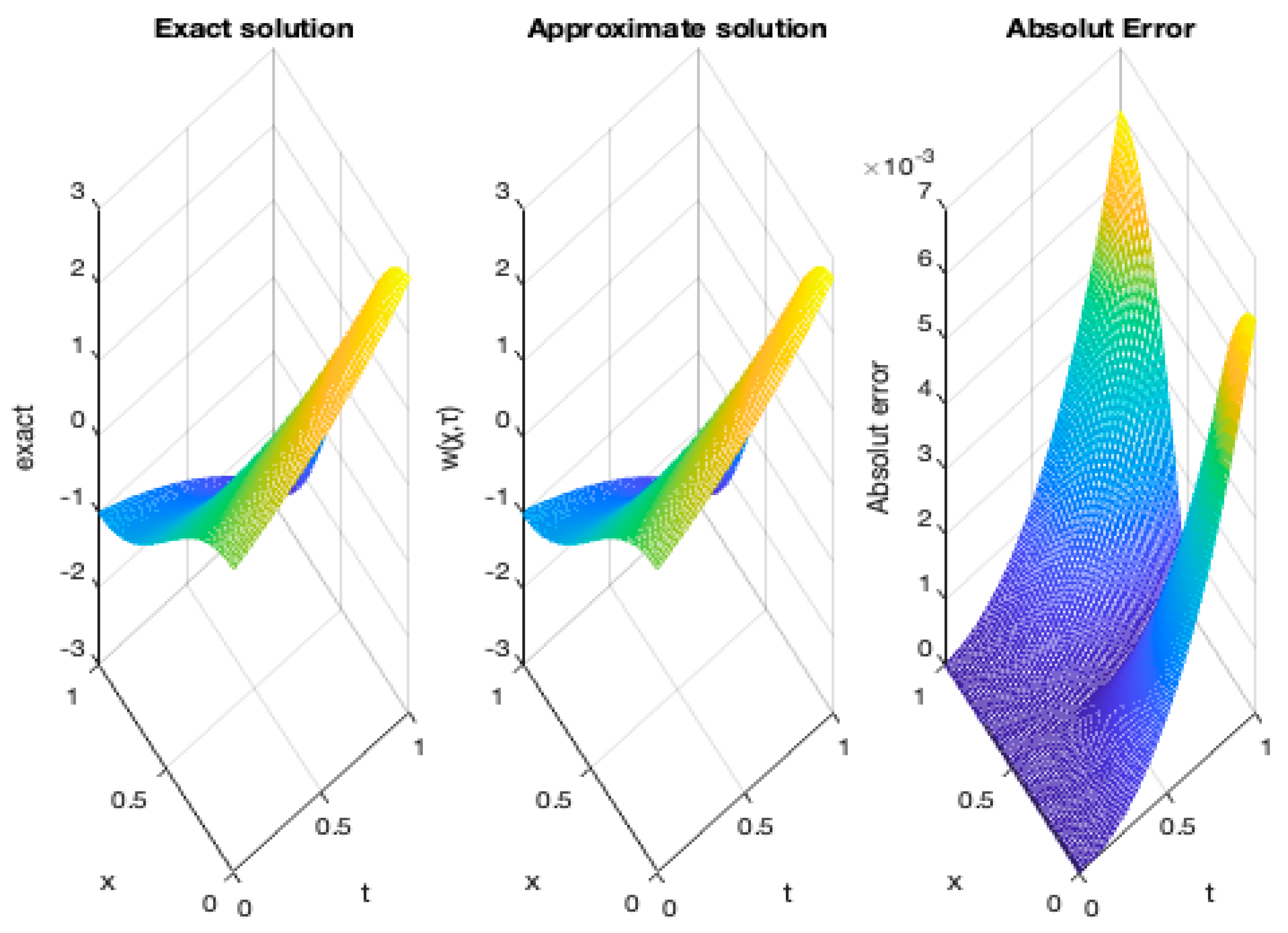
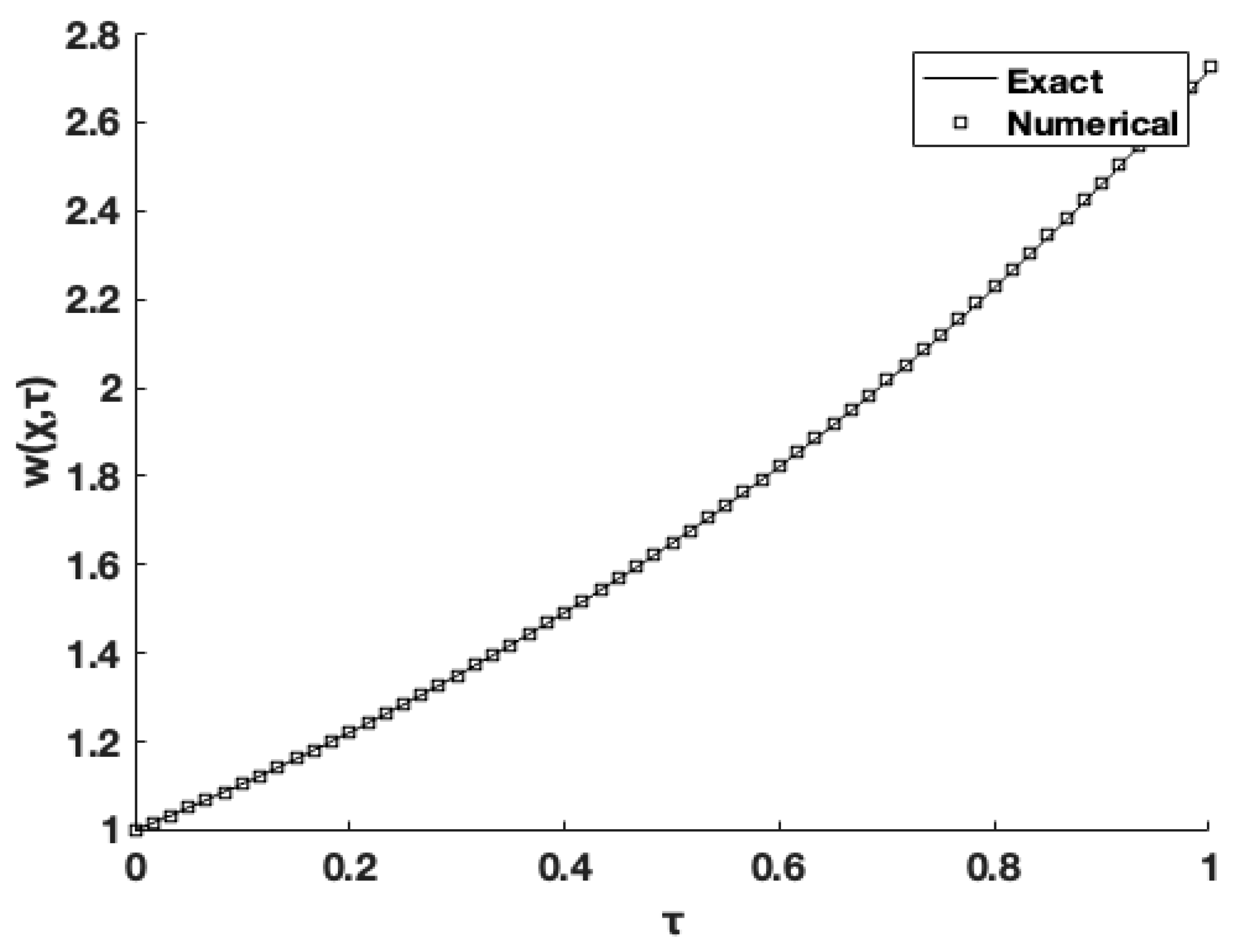
By substituting it into the governing equation, the proposed solution can be verified. The precise and numerical solution for $\mathcal{w}\left(\chi , \tau \right)$, with grid size $M=N=60,$ is shown in Figure 1, with the absolute error graph showing very good precision of approximately $O\left({10}^{-3}\right)$ magnitude (see the results in the right-side plot). Excellent agreement is also found when comparing the computationally necessary data with the analytical information for $\mathcal{w}\left(0, \tau \right)$ and for $\alpha =0.0001$ in Figure 2.

4. Numerical Method for Solving the IP (1)–(5)

The objective of this section is to address the solution to the IP. To determine stable reconstructions for the unknown coefficient $a\left(t\right)$ in conjunction with the transverse displacement, $\mathcal{w}\left(\chi ,\tau \right)$, such that Equations (1)–(5) are satisfied. Nevertheless, due to the ill-posed characteristics of the IP, the solution exhibits considerable sensitivity to noise; thus, minor flaws in the input data may result in substantial errors in the solution. Consequently, the Tikhonov regularization approach is used to provide an accurate and stable solution; refer to [40,41] for further details. According to condition (5), the Tikhonov regularization functional is formulated as follows:

$$\mathrm{K}\left(\underset{\_}{a}\right)={‖\mathcal{w}\left(0, \tau \right)-h\left( \tau \right)‖}^2+\mathsf{\vartheta }\Vert a( \tau ){\Vert }^2 ,$$

(39)

and the approximate formula is given by

$$K\left(\underset{\_}{a}\right)={\displaystyle {\sum }_{\mathrm{n}=1}^N} {\left(\mathcal{w}\left(0,{ \tau }_n\right)-h\left({ \tau }_n\right)\right)}^2+\mathsf{\vartheta }{\displaystyle {\sum }_{\mathrm{n}=1}^N} a_n^2,$$

(40)

where $\mathsf{\vartheta }\ge 0$ is the regularization parameter. The MATLAB optimization toolbox function lsqnonlin minimizes the objective function (39) from the initial guess, and we attempt to solve the nonlinear least squares curve fitting problem using this method. The potential term $a\left(\tau \right)$ has lower and upper bounds of ${10}^{-2}$ and ${10}^2$, respectively.

A numerical simulation of the noisy (perturbed) data is established as

$$‖h^{\delta }-h‖\le \delta .$$

(41)

The perturbation term $\delta$ is an independent normally distributed random variable with a mean of zero and a standard deviation $\sigma$. This standard deviation is defined proportionally to the maximum amplitude of the exact data.

$$\sigma =p\times \underset{ \tau \in [0,T]}{\mathrm{m}\mathrm{a}\mathrm{x}} |h(\tau )|,$$

(42)

where $p$ represents the designated noise level ratio. Computationally, the random noise vector $\delta ={({\delta }_0,\dots ,{\delta }_N)}^T$ is generated using MATLAB^® R2023a normal random number generator as follows:

$$\delta =\mathrm{n}\mathrm{o}\mathrm{r}\mathrm{m}\mathrm{r}\mathrm{n}\mathrm{d}(0,\sigma ,N).$$

5. Numerical Outputs and Discussion

The root means square error ($rmse$) is anticipated to test the precise computational outputs obtained by the Tikhonov regularization process, according to the following expression:

$$rmse\left(a\right)=\sqrt{{\displaystyle \frac{1}{N}}{\displaystyle \sum _{\mathrm{n}=1}^N} {\left(a^{\mathrm{numerical}}\left({\tau }_n\right)-a^{\mathrm{exact}}\left({\tau }_n\right)\right)}^2}$$

(43)

• Example 1: Recovery of Smooth Potential Term

Examine the IP (1)–(5) with $T=1$ and $\alpha =0.0001$, along with the subsequent given data.

$$\begin{array}{l}\varphi (\chi )=-{\displaystyle \frac{\cos (2\pi \chi )}{e}}, \psi (\chi )={\displaystyle \frac{\cos (2\pi \chi )}{e}}, \chi \in \left[\mathrm{0,1}\right],\\ G\left(\chi ,\tau \right)=e^{-\sqrt{1+\tau }}cos\left(2\pi \chi \right)\left[-0.155855-{\displaystyle \frac{1}{4{\left( \tau +1\right)}^{\raisebox{1ex}{$3$}\!\left/ \!\raisebox{-1ex}{$2$}\right.}}}-{\displaystyle \frac{1}{4\left( \tau +1\right)}}+\cos \left(4\pi \tau \right)\right], (\chi , \tau )\in Q_T,\\ h\left(\tau \right)=-e^{\sqrt{1+} \tau } , \tau \in \left[0,T\right].\end{array}$$

The solution’s uniqueness is guaranteed by the fulfillment of the requirements outlined in [34]. The precise solution for this example is provided below:

$$\mathcal{w}\left(\chi , \tau \right)=-e^{-\sqrt{1+} \tau }\cos \left(2\pi \chi \right) \left(\chi , \tau \right)ϵQ_T, a(\tau )=\cos \left(4\pi \tau \right), \tau \in [0,T],$$

(44)

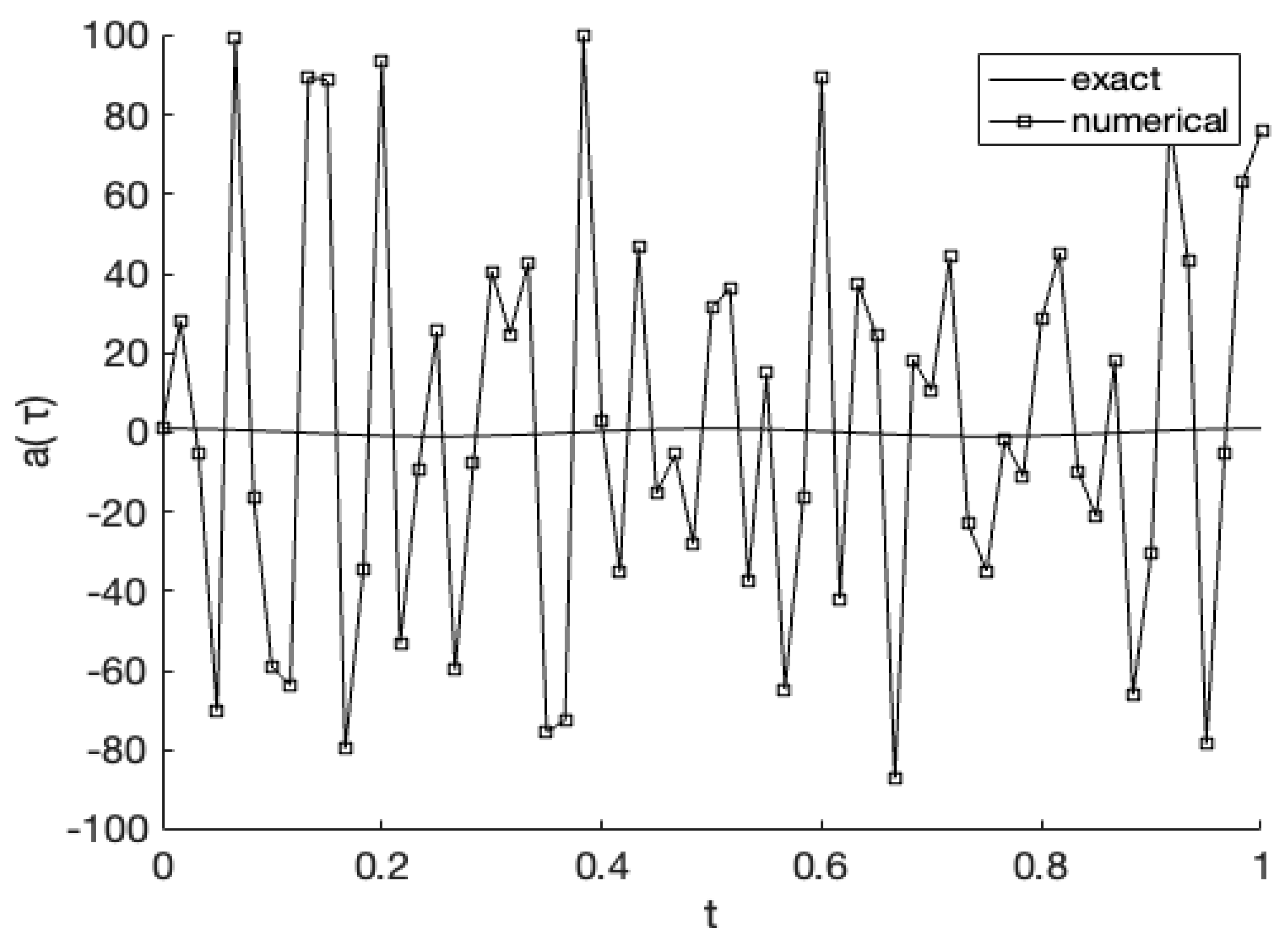
The preliminary estimate was adopted as $a\left(0\right)=1.$ It is straightforward to demonstrate that the given information fulfills the conditions specified in [34], guaranteeing a unique solution to IPs (1)–(5). The computational solution without noise is discussed for $p= 0$, meaning that (42) has no noise.

Table 1. The numerical and precise values for the intended output $a\left(\tau \right)$ compared at different time nodes with grid sizes $M=N=\left\{\mathrm{10,20,40,60,80}\right\}$, with $\mathsf{\vartheta }=0,p=0$.

$\mathit{\tau }$	0.1	0.2	0.3	0.4	0.5	0.6	0.7	0.8	0.9
$M=N=10$	0.3130	−0.7649	−0.8153	0.3395	0.9961	0.3260	−0.8125	−0.8046	0.3193
$M=N=20$	0.3504	−0.7730	−0.7974	0.3143	1.0075	0.3148	−0.8060	−0.8025	0.3122
$M=N=40$	0.3438	−0.7941	−0.8003	0.3139	1.0024	0.3138	−0.8068	−0.8074	0.3108
$M=N=60$	0.3320	−0.8022	−0.8087	0.3129	1.0039	0.3096	−0.8051	−0.8073	0.3081
$M=N=80$	0.3090	−0.8090	−0.8090	0.3090	1.000	0.3090	−0.8090	−0.8090	−0.3090
Exact	0.3090	−0.8090	−-0.8090	0.3090	1.000	0.3090	−0.8090	−0.8090	0.3090

shows that there is strong agreement between the analytical and approximation solutions for the coefficient $a\left(\tau \right)$ obtained with diverse values of $M$ and $N$. Figure 3 plots the associated results for this case, showing excellent agreement. Figure 4 illustrates the objective function (40), and a decelerating convergence is observed, as a stationary value of approximately $O\left({10}^{-11}\right)$ is obtained after no more than 10 iterations.

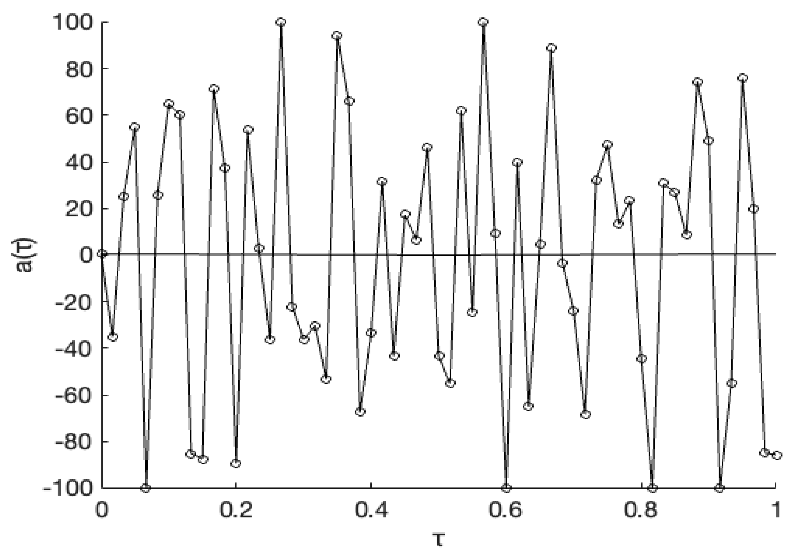
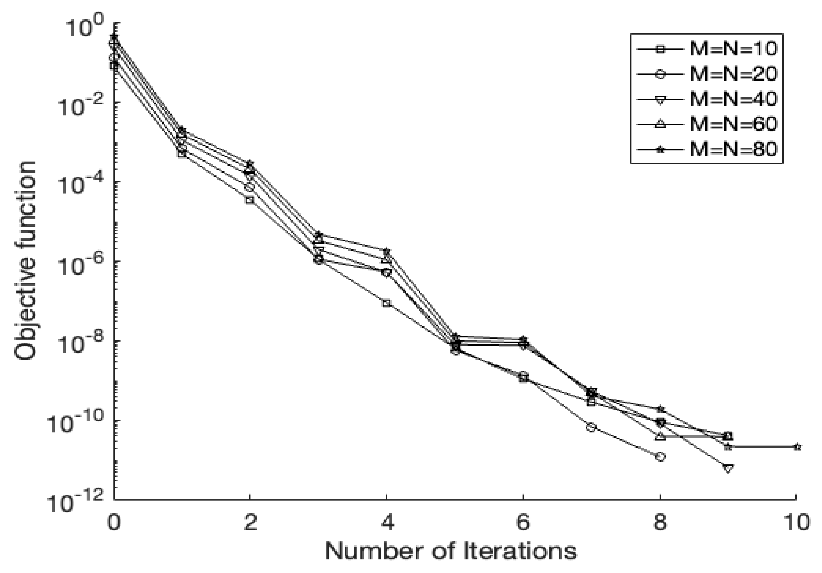
Now, we investigate the reconstruction of potential term a($\tau$) without regularization (i.e., $\mathsf{\vartheta }=0$) and with measurement noise of magnitude p = 1% in input data (5) added as shown in (41). The obtained results are presented in Figure 5 and Figure 6. The numerical and precise answers for the potential term a($\tau$) are compared in Figure 5. Due to the problem’s ill-posedness, the numerical results exhibit significant deviations and pronounced oscillations, which are indicative of instability and limited accuracy. Figure 6 plots the objective function related to this case. Despite the objective function decreasing monotonically and reaching a relatively small value (about ${10}^{-3}$) in the initial iterations, the corresponding solution remains unstable and inaccurate.

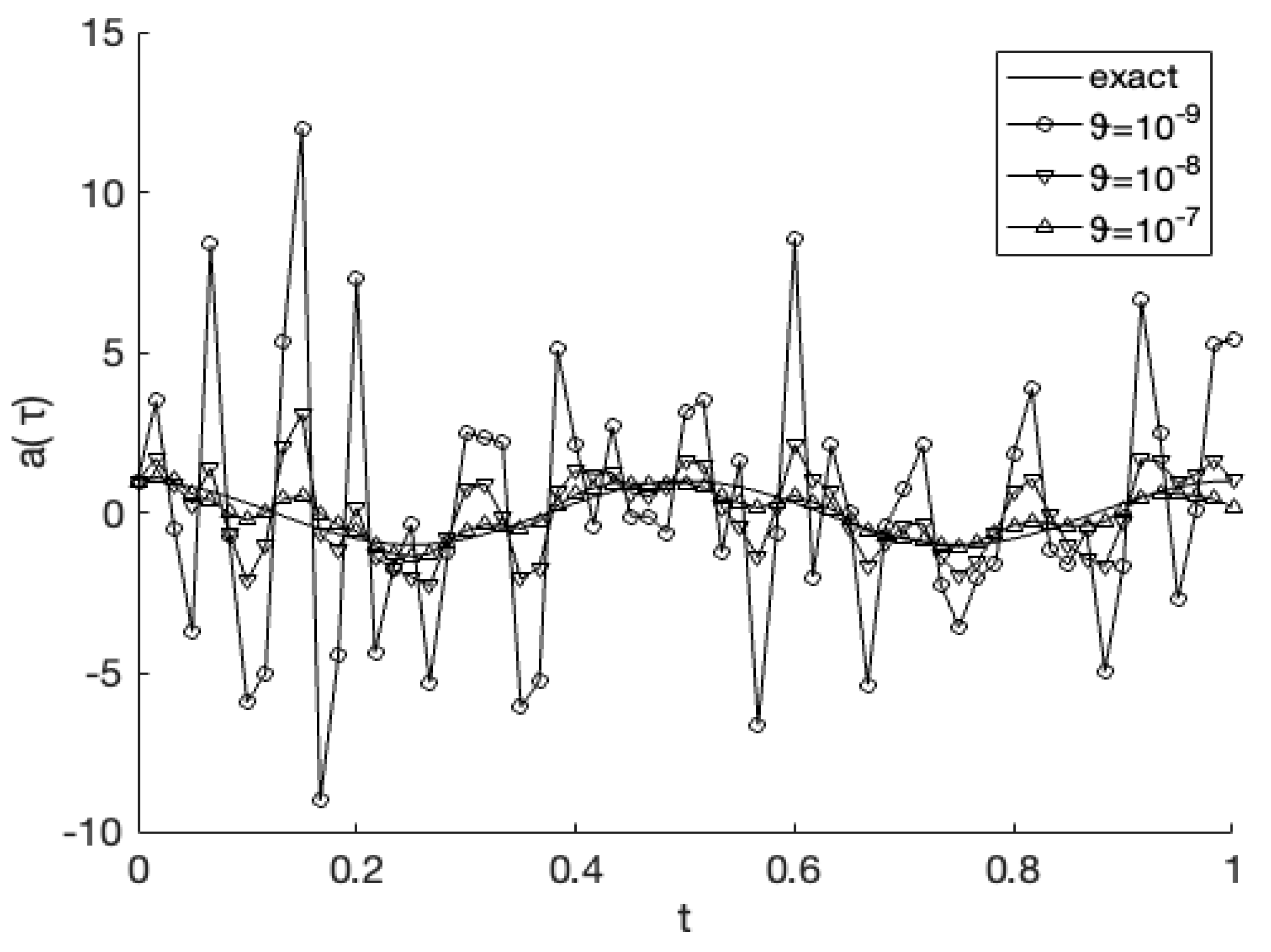
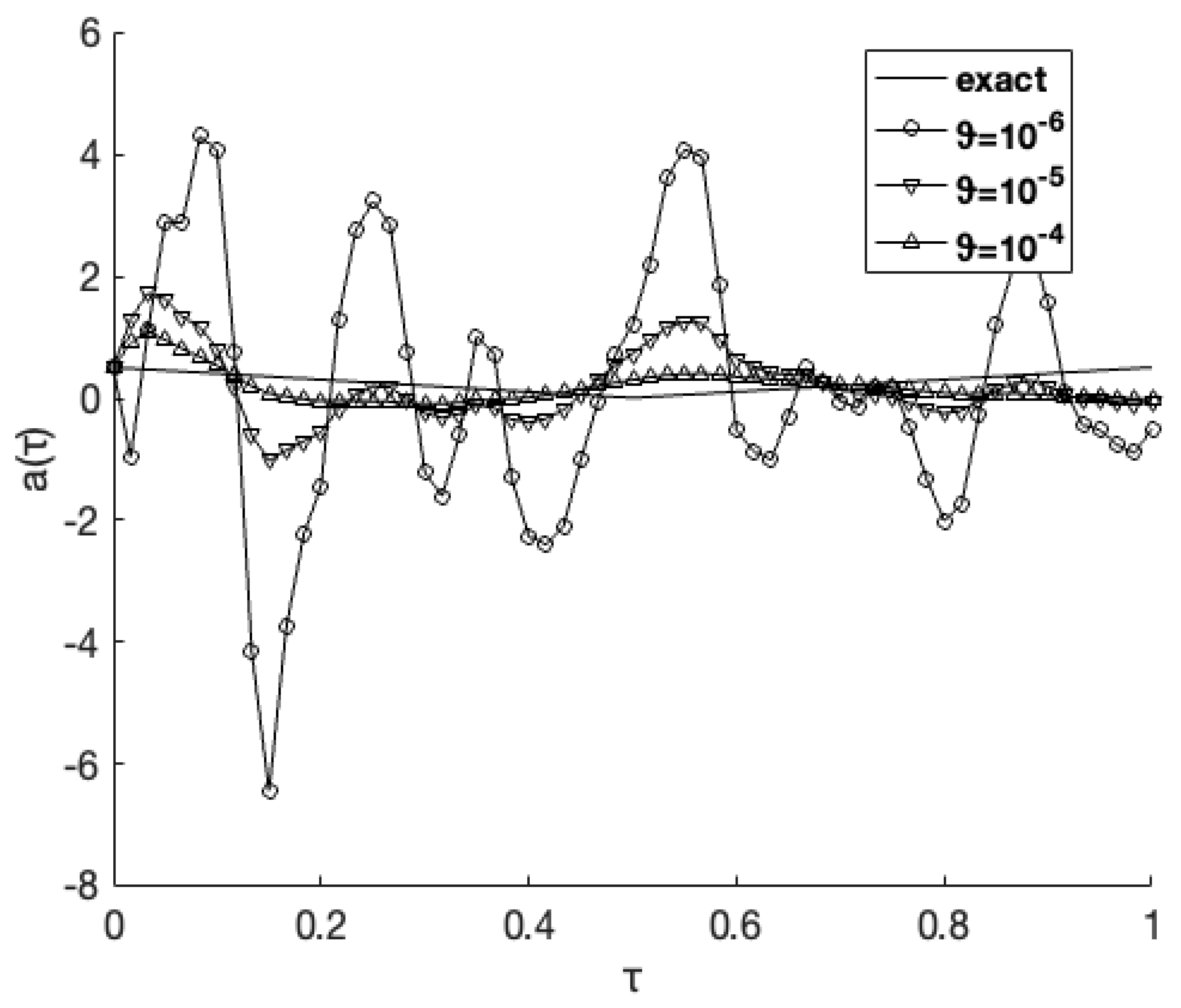
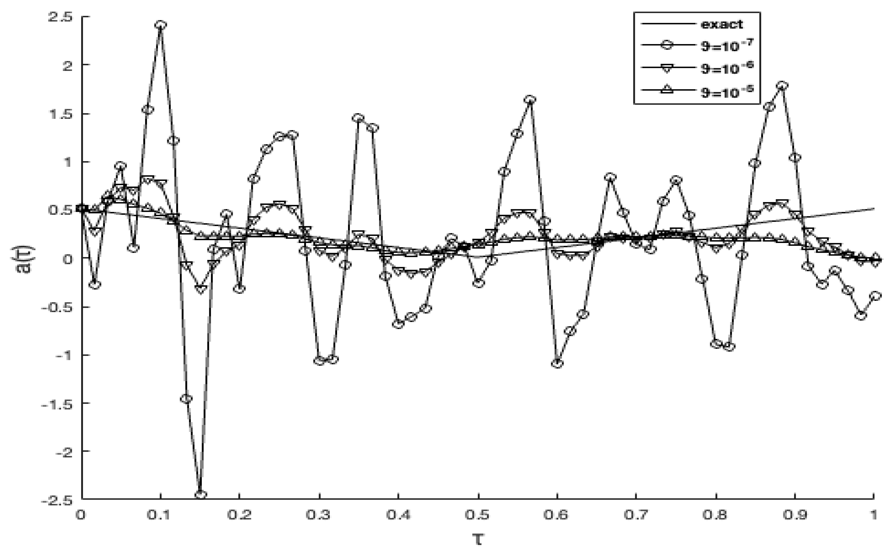
The exact and reconstructed results for a($\tau$) for diverse values of regularization parameters $\mathsf{\vartheta }$ and noise levels are shown in Figure 7, Figure 8, Figure 9 and Figure 10, with 1% noise, $\mathsf{\vartheta }$ ∈ {10⁻⁶, 10⁻⁵, 10⁻⁴}. Figure 7 and Figure 8 show that bigger $\mathsf{\vartheta }$ values provide smoother but more biased results, whereas smaller $\mathsf{\vartheta }$ values produce solutions that are closer to the correct curve but have more oscillations because of noise sensitivity. When very small values of $\mathsf{\vartheta }$ (e.g., 10⁻⁶) are used, the objective function in Figure 8 significantly decreases. However, for p = 0.1% noise ($\mathsf{\vartheta }$ ∈ {10⁻⁹, 10⁻⁸, 10⁻⁷}), such small $\mathsf{\vartheta }$ values cause large oscillations because of noise amplification.

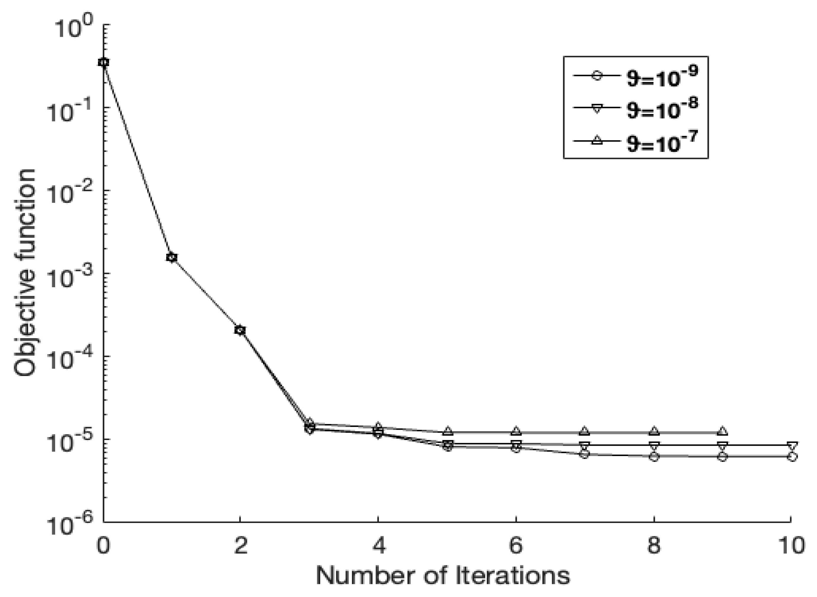
In Figure 9 and Figure 10, greater $\mathsf{\vartheta }$ = 10⁻⁷ reduces these oscillations, producing smoother but less detailed solutions. With very small differences in $\mathsf{\vartheta }$ values, the corresponding objective function curves (see Figure 10) converge quickly and stabilize after approximately three iterations, indicating that $\mathsf{\vartheta }$ has a greater impact on reconstruction accuracy than on convergence speed.

Table 2. Computational information obtained from Lsqnonlin routine output during minimization processes for Example 1 with $p=1\%$ noise contaminated in (5) via (41).

$\mathit{p}=1\%$	$\mathsf{\vartheta }={10}^{-7}$	$\mathsf{\vartheta }={10}^{-6}$	$\mathsf{\vartheta }={10}^{-5}$	$\mathsf{\vartheta }={10}^{-4}$	$\mathsf{\vartheta }={10}^{-3}$	$\mathsf{\vartheta }={10}^{-2}$	$\mathsf{\vartheta }={10}^{-1}$
Count of iterations	11	8	18	5	4	4	3
No. of evaluations	744	588	1178	372	310	310	248
Objective function	0.00096	0.00010	0.00106	0.00109	0.00110	0.001108	0.001109
$rmse$($a$)	2.7341	0.7753	0.6782	0.7027	0.7064	0.7070	0.7071
Computational time (s)	78.5	59.25	124.78	39.55	33.95	33.74	25.67

and

Table 3. Computational information obtained from Lsqnonlin routine output during minimization processes for Example 1 with $p=0.1\%$ noise contaminated in (5) via (41).

$\mathit{p}=0.1\%$	$\mathit{\vartheta }={10}^{-9}$	$\mathit{\vartheta }={10}^{-8}$	$\mathit{\vartheta }={10}^{-7}$	$\mathit{\vartheta }={10}^{-6}$	$\mathit{\vartheta }={10}^{-5}$	$\mathit{\vartheta }={10}^{-4}$	$\mathit{\vartheta }={10}^{-3}$	$\mathit{\vartheta }={10}^{-2}$	$\mathit{\vartheta }={10}^{-1}$
Count of iterations	10	10	9	8	23	6	4	11	3
No. evaluations	682	682	620	558	1488	434	310	744	248
Objective function	6.23 × 10−6	6.23 × 10−6	1.2 × 10−5	2.83 × 10−5	8.46 × 10−5	0.00013	0.00015	0.00016	0.00016
$rmse$($a$)	2.7341	2.7341	0.3087	0.3133	0.5292	0.6769	0.7034	0.7067	0.7071
Computational time (s)	74.17	72.38	65.69	63.64	159.12	45.99	32.22	78.88	25.76

present the numerical outputs, including the number of iterations, the number of function evaluations, the final value of the convergent objective function (40), and the root mean square error ($rmse$) for Example 1. The results reveal that an acceptable range of data can be achieved with a minimal $rmse\left(a\right)$ value. These tables show that, in all cases, the computational time exceeded 160 s. at the smallest $rmse\left(a\right)$ value.

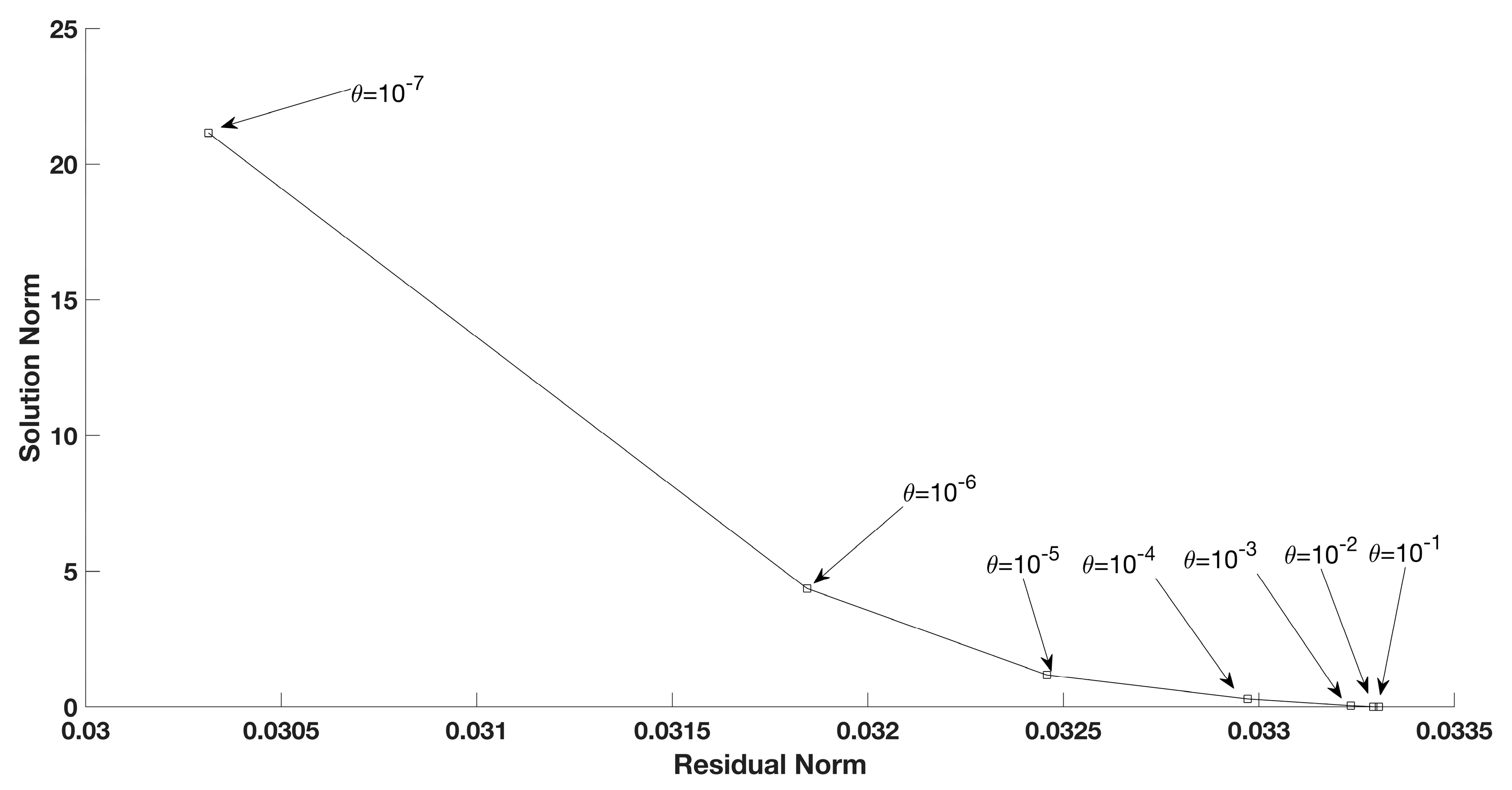
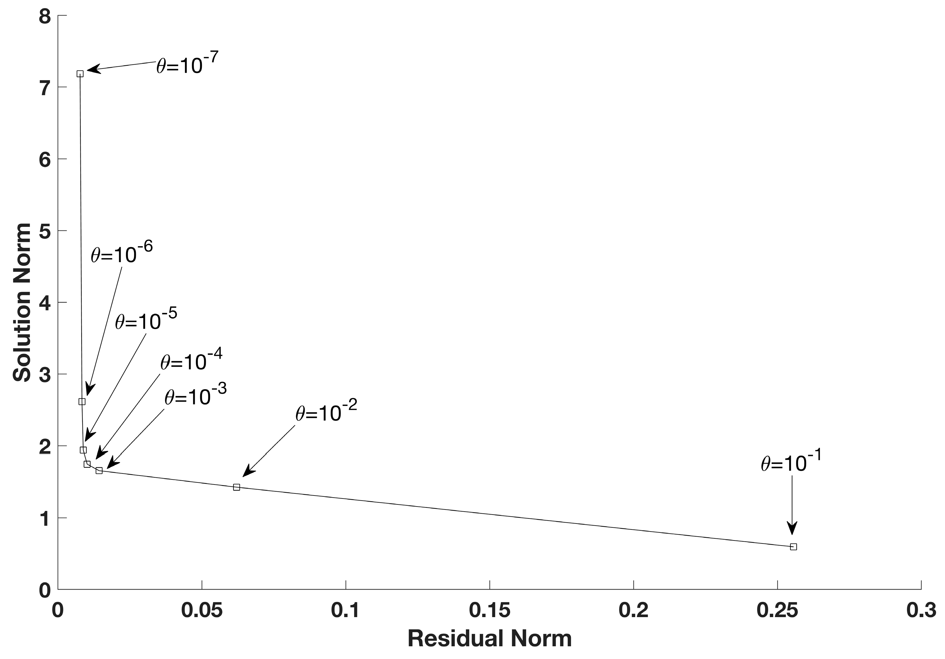
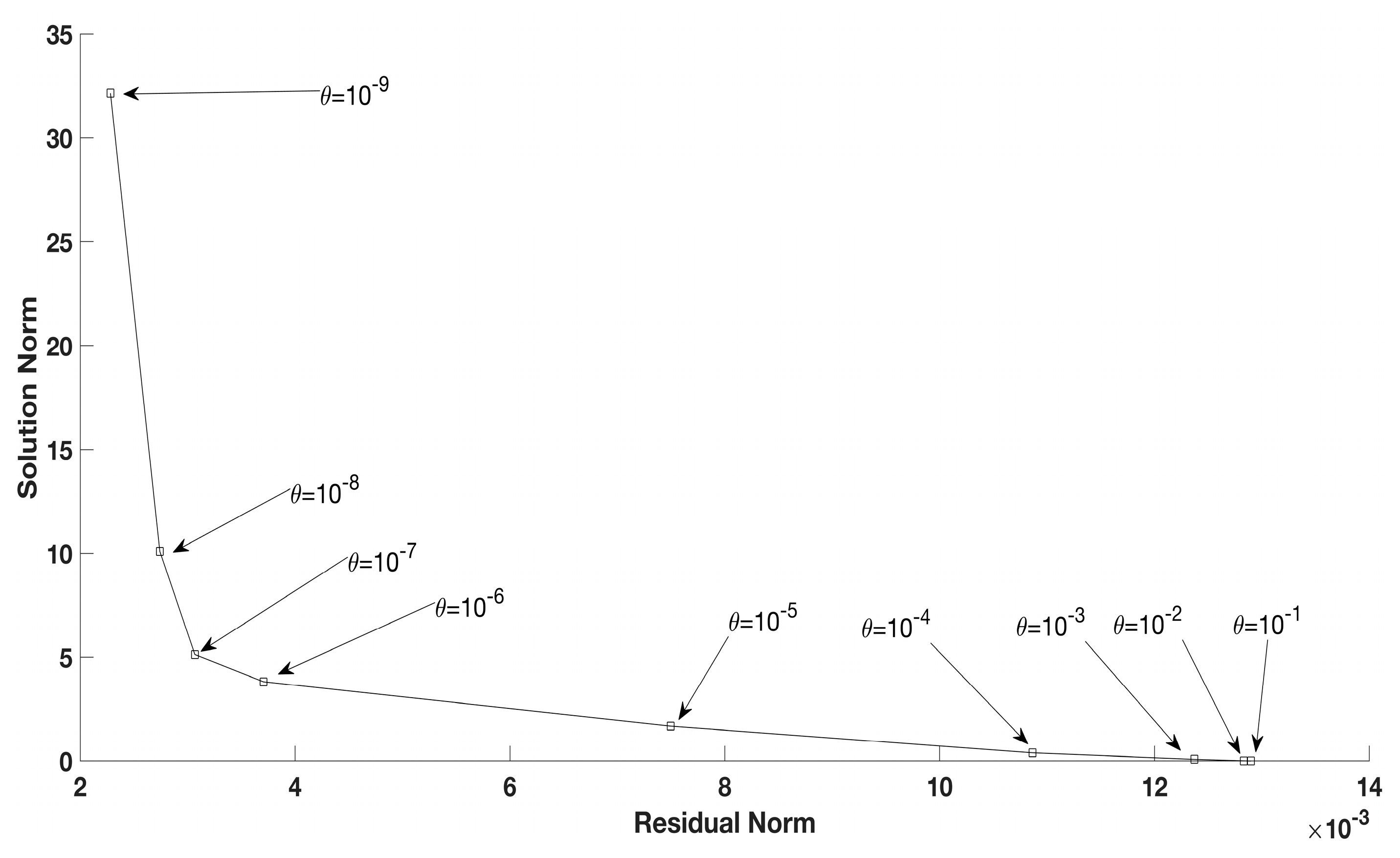
The L-curve plot is an effective instrument for selecting the appropriate regularization parameter for the specified data in the regularization process. The L-curve is derived from a log–log plot of the residual norm $‖\mathcal{w}\left(0,\tau \right)-h\left(\tau \right)‖$ against the corresponding regularized solution norm $‖a‖$. It is a suitable graphical tool for illustrating the trade-off between the size of a regularization’s solution and the fit of the provided data [42,43]. Figure 11 depicts the distinctive L-shaped behavior of the curve. The vertical branch pertains to rather substantial regularization parameters, resulting in excessively smoothed solutions. Conversely, the horizontal branch is associated with extremely small regularization parameters, resulting in unstable solutions that are highly susceptible to noise. Consequently, a perfect regularization parameter is chosen at the vertex of the L-curve, as this position signifies the optimal balance between reducing the residual norm and preserving the stability of the solution. According to Figure 12, the values

$$\mathsf{\vartheta }=\left\{{10}^{-6},{10}^{-7}\right\}$$

are situated at the curve’s intersection and offer appropriate regularized solutions. Nonetheless, the value $\mathsf{\vartheta }={10}^{-7}$ is the most suitable option as it is nearest to the inflection point of the L-curve.

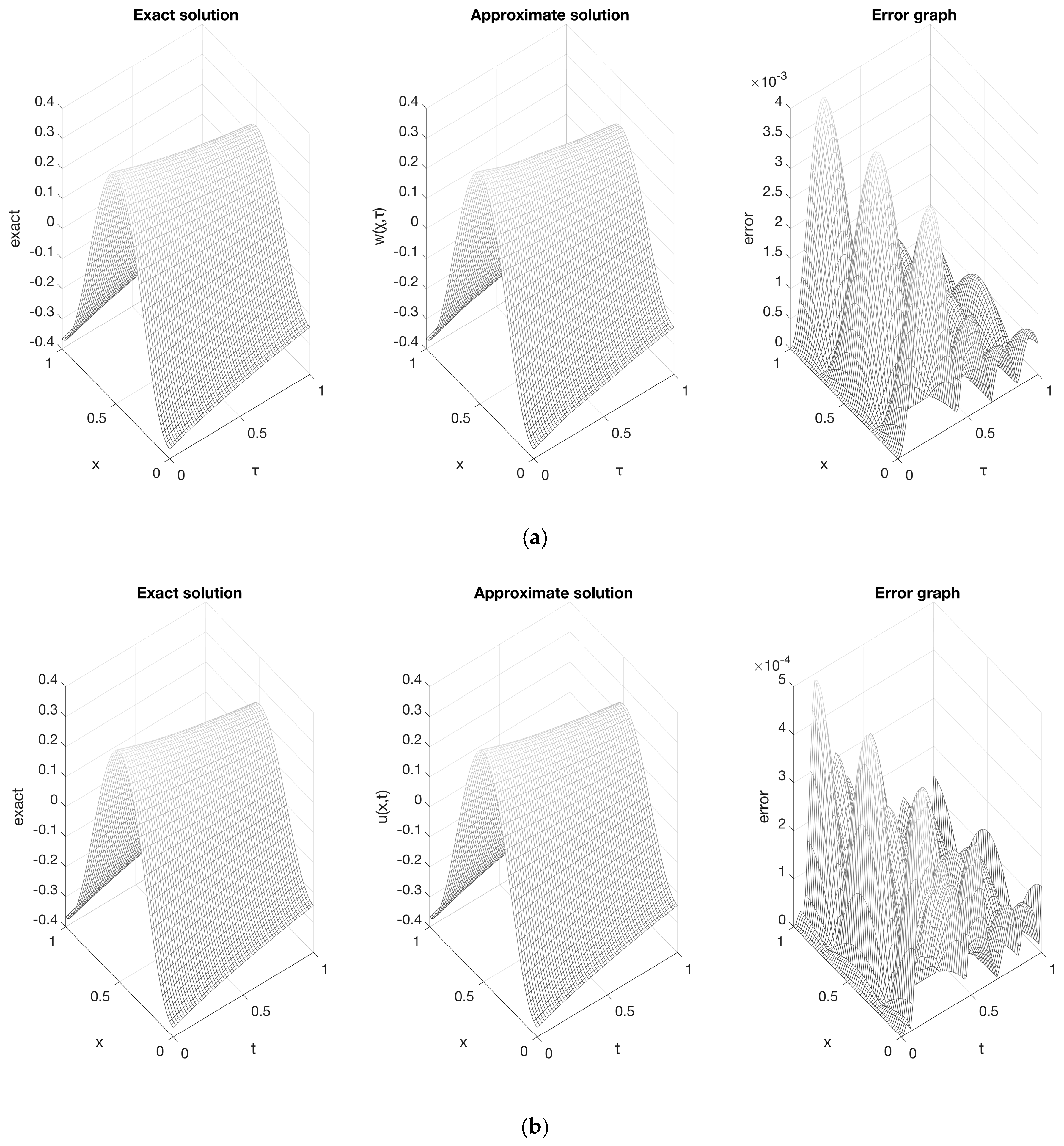
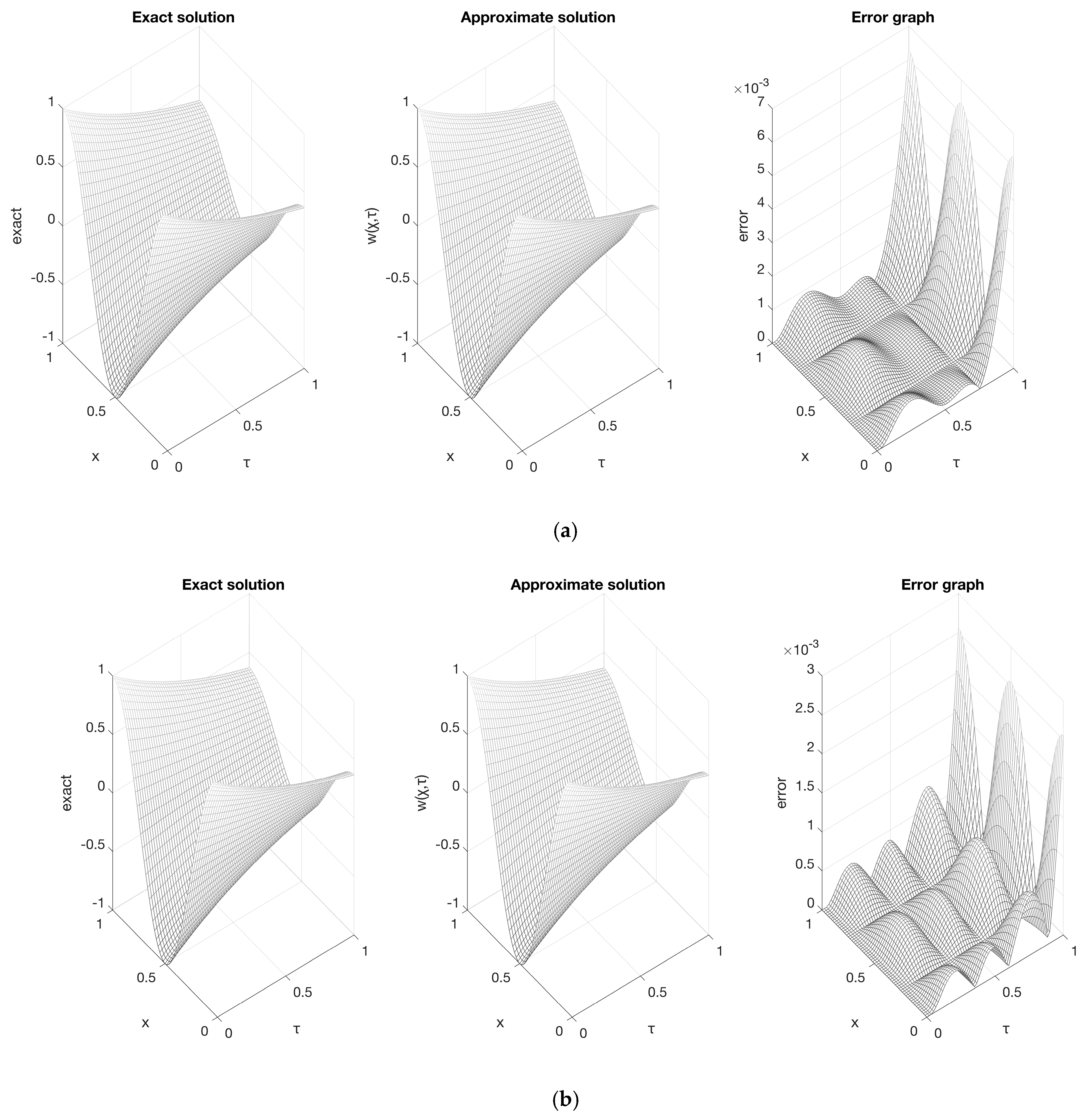
Figure 13 represents the plot of transverse displacement distribution for the case (a) $\mathsf{\vartheta }={10}^{-5} ,p=1\%$ (b) $\mathsf{\vartheta }={10}^{-7} ,p=0.1\%$. This figure shows that there outstanding retrievals for $\mathcal{w}\left(\chi , \tau \right)$ are obtained with a magnitude of $O\left({10}^{-3}\right)-O\left({10}^{-4}\right)$ of maximum error (see the third column in Figure 13).

• Example 2: Non-smooth Potential Term

In this example, we examine the non-smooth potential coefficient $a\left(\tau \right)$ and solve IPs (1)–(4) with $T=1$ and $\alpha =0.0001,$ with the next input data

$$\begin{array}{l}\mathcal{w}\left(\chi ,0\right)=\cos (2\pi \chi ) , {\mathcal{w}}_{\tau }(\chi ,0)=-\mathit{cos}(2\pi \chi ) \chi \in \left[\mathrm{0,1}\right],\\ G\left(\chi , \tau \right)=e^{-\tau }cos\left(2\pi \chi \right)\left[ 1.14585-| \tau -0.5| \right] (\chi , \tau )\in Q_T ,\end{array}$$

whereas the exact potential term is

$$a\left(\tau \right)=0.01+\left| \tau -0.5\right|, \tau \in \left[0,T\right],$$

(45)

and the precise solution is given by

$$\mathcal{w}\left(\chi , \tau \right)=e^{-\tau }\cos \left(2\pi \chi \right), \left(\chi ,\tau \right)ϵQ_T,$$

(46)

and the overdetermination condition is

$$\mathcal{w}\left(0,\tau \right)=h\left(\tau \right)=e^{-\tau }, \tau \in \left[0,T\right].$$

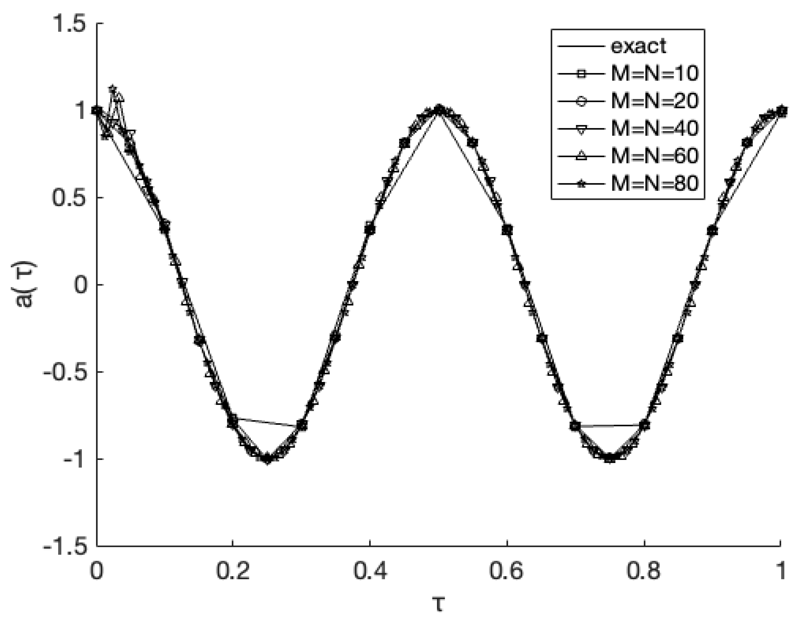
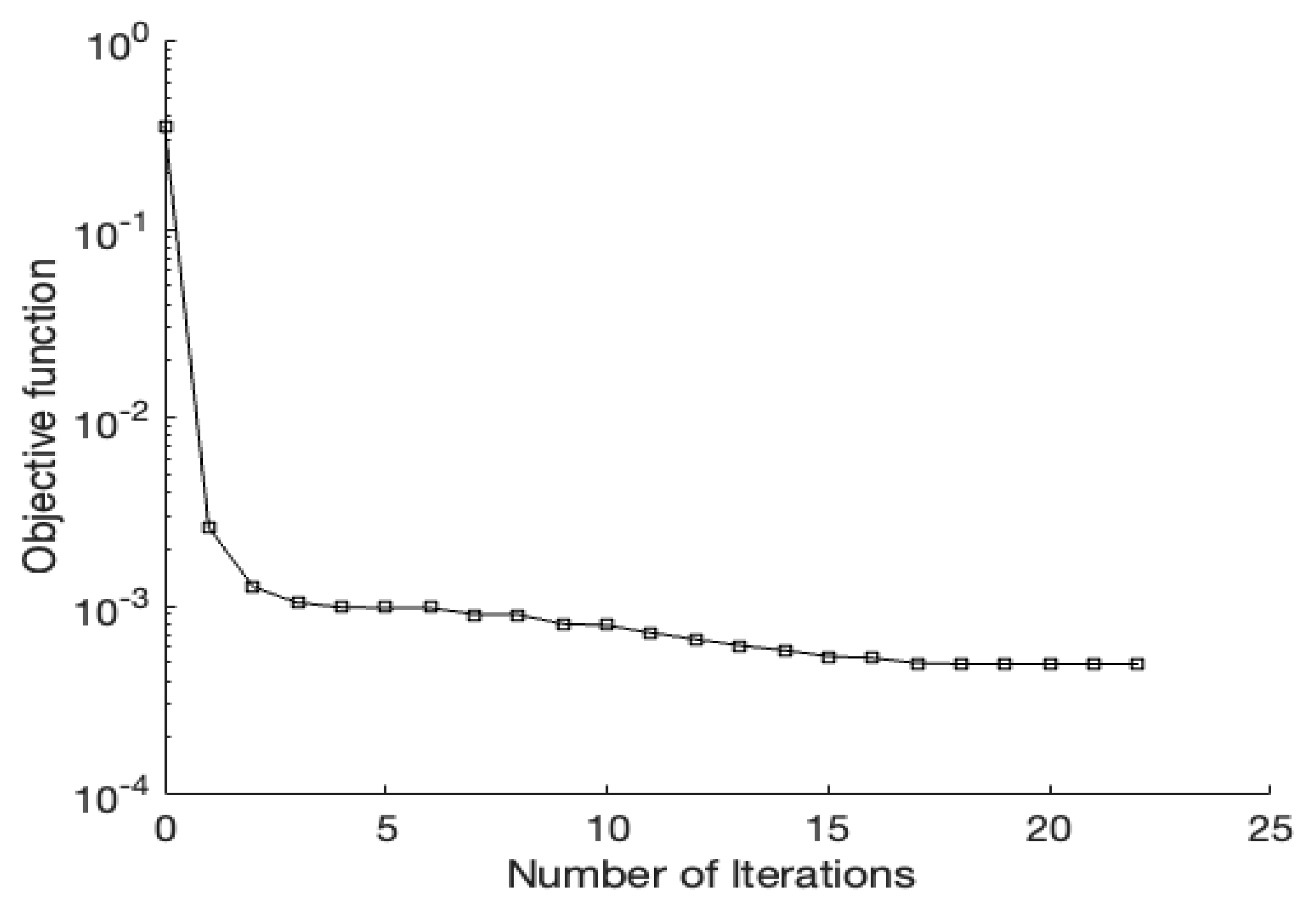
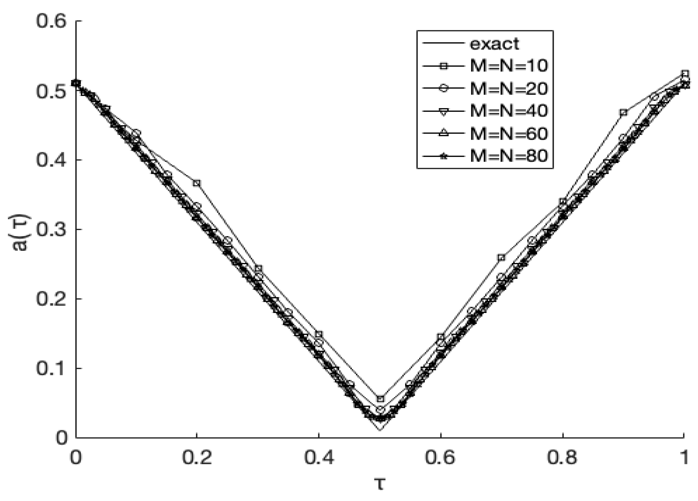
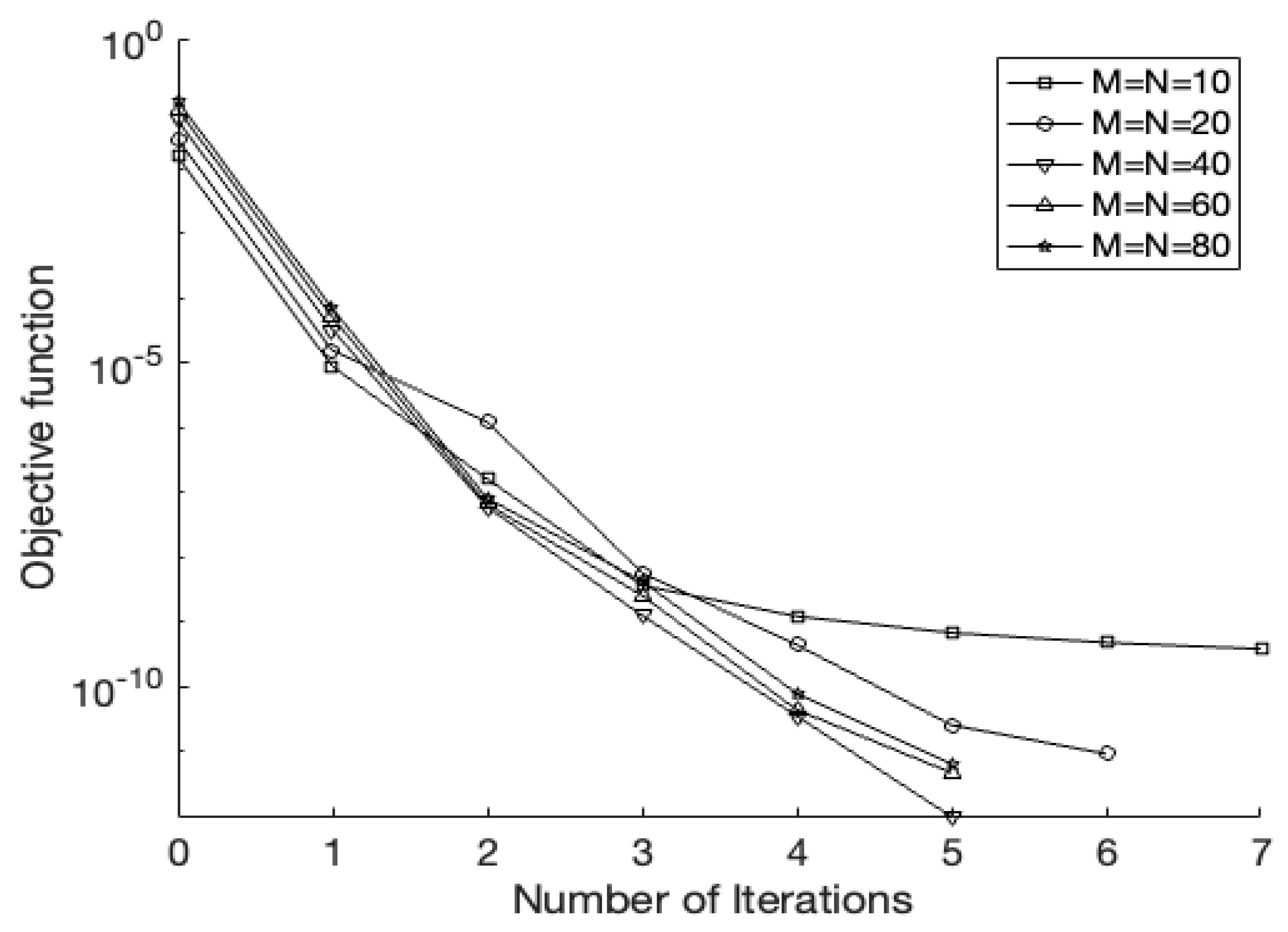
Now, $a\left(0\right)=0.51$ is used as the preliminary estimate. For $p=0\%$, the recovery of an unknown term without noise is examined. The corresponding results for the given case are plotted in Figure 14, showing strong agreement. Figure 15 shows the objective function (40), with speed convergence to extremely low values of order $O\left({10}^{-12}\right)$ in no more than seven iterations. It should be reported that minimization processes stop when either the solution or objective function accuracy are achieved. Figure 14 and

Table 4. The precise numerical values for the intended output $a\left(\tau \right)$ compared at different time nodes with grid sizes. $M=N=\left\{\mathrm{10,20,40,60,80}\right\}$ with $\mathsf{\vartheta }=0,p=0\%$.

$\mathit{\tau }$	0.1	0.2	0.3	0.4	0.5	0.6	0.7	0.8	0.9
$M=N=10$	0.4281	0.3669	0.2447	0.1498	0.0554	0.1448	0.2590	0.3396	0.4679
$M=N=20$	0.4392	0.3329	0.2324	0.1360	0.0396	0.1360	0.2314	0.3339	0.4319
$M=N=40$	0.4219	0.3222	0.2223	0.1218	0.0284	0.1222	0.2226	0.3220	0.4208
$M=N=60$	0.4180	0.3179	0.2178	0.1198	0.0339	0.1198	0.2173	0.3186	0.4176
$M=N=80$	0.4160	0.3160	0.2158	0.1178	0.0272	0.1178	0.2153	0.3417	0.4151
Exact	0.4100	0.3100	0.2100	0.1100	0.0100	0.1100	0.2100	0.3350	0.4100

show that as $M=N$ increases, the accuracy also improves, revealing mesh independence. Therefore, we take $M=N=60$ as the affixed mesh size.

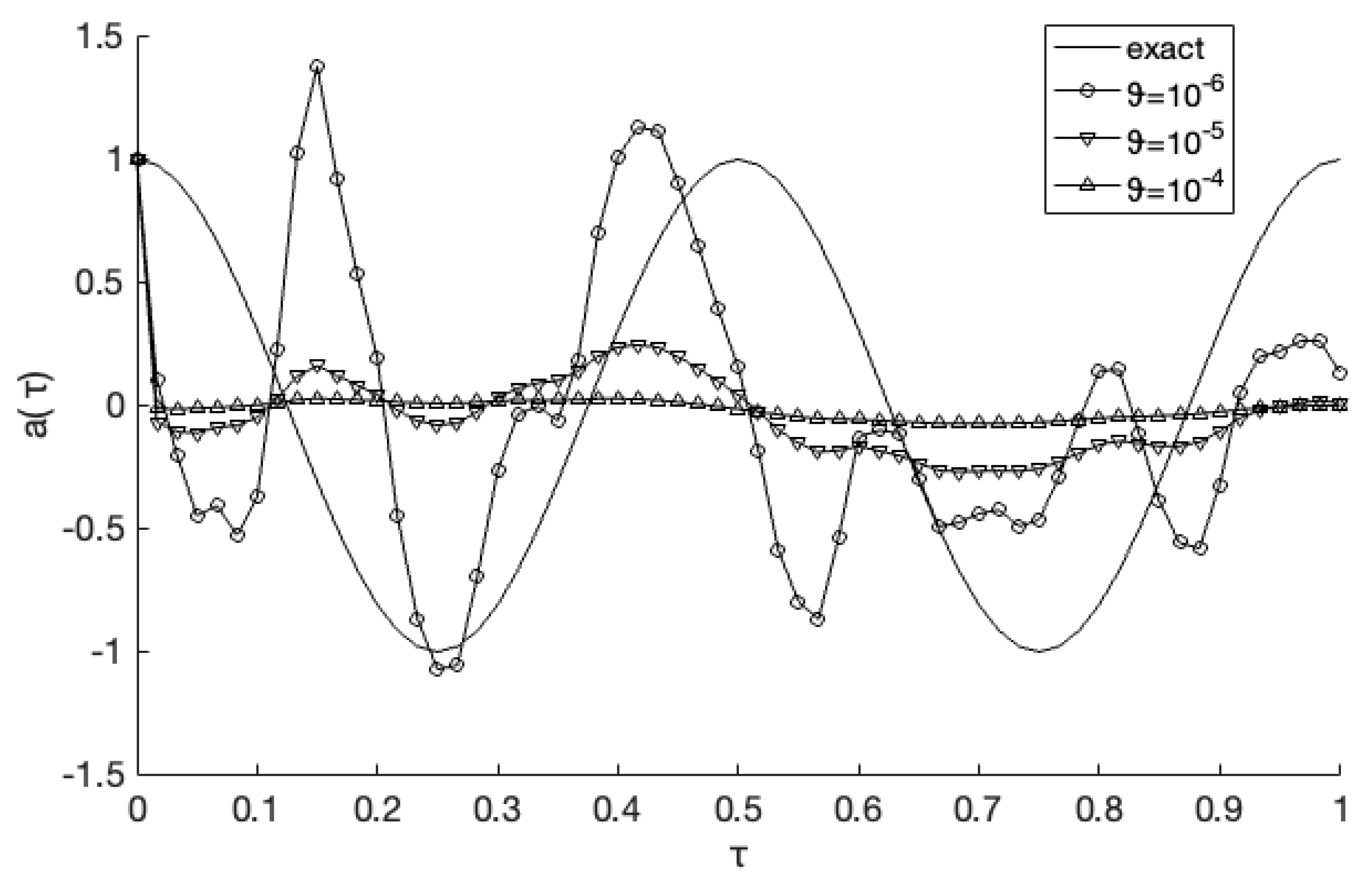
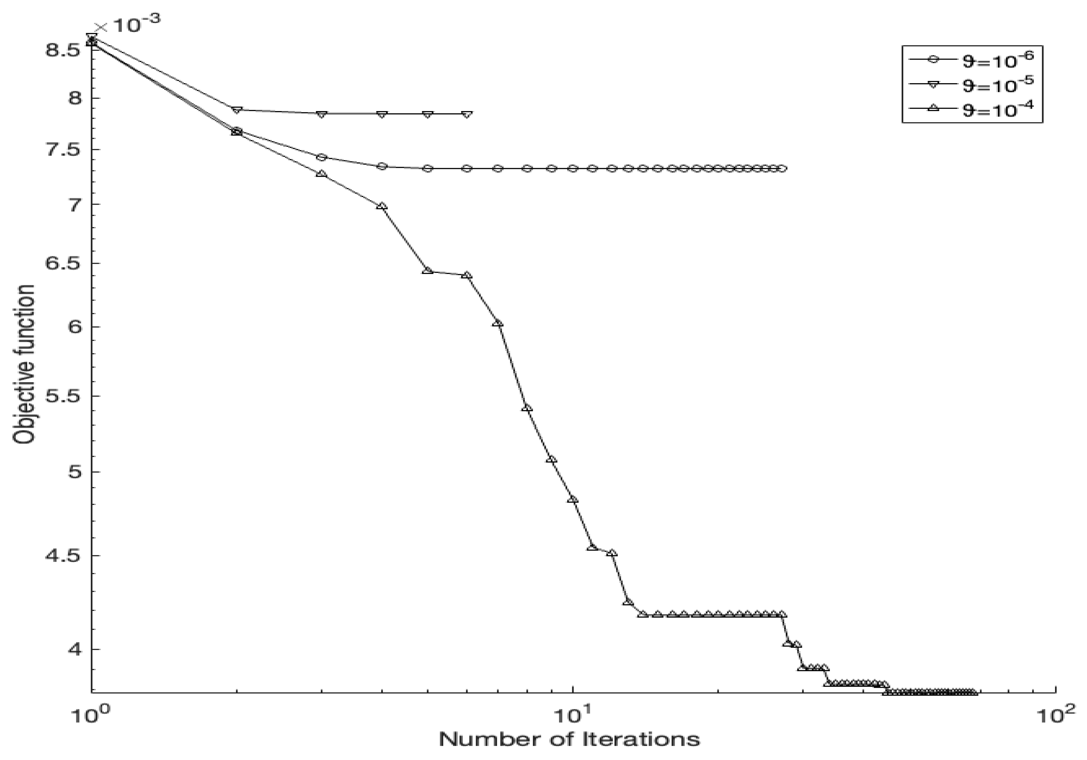
Due to noise, the solution is extremely oscillatory and unstable when no regularization is applied, as explained in Figure 16. Stability can be restored by adding a regularization term (see Figure 17 and Figure 18). Larger $\mathsf{\vartheta }$ values reduce oscillations with little deviation, while smaller $\mathsf{\vartheta }$ values increase accuracy but introduce more noise. The solutions are near to the exact curve when noise levels are reduced. Figure 17 shows that suitable regularization parameters guarantee accurate and consistent results.

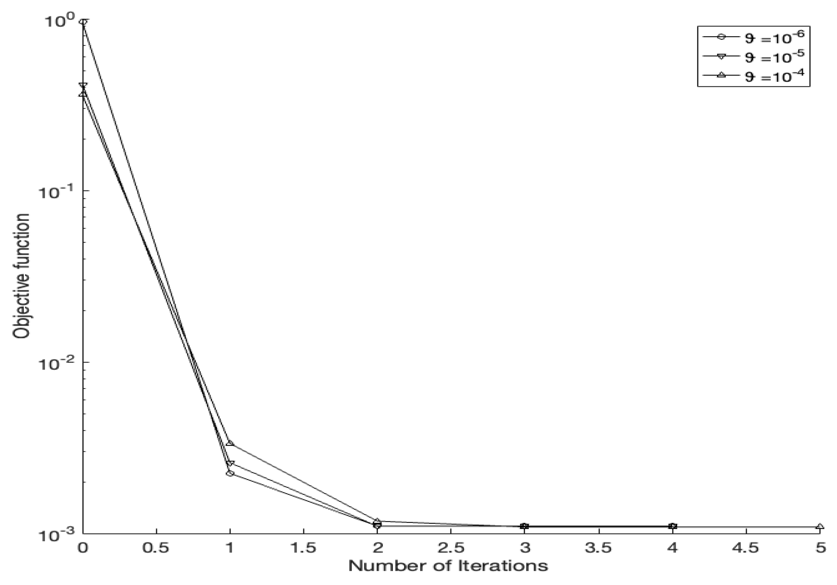
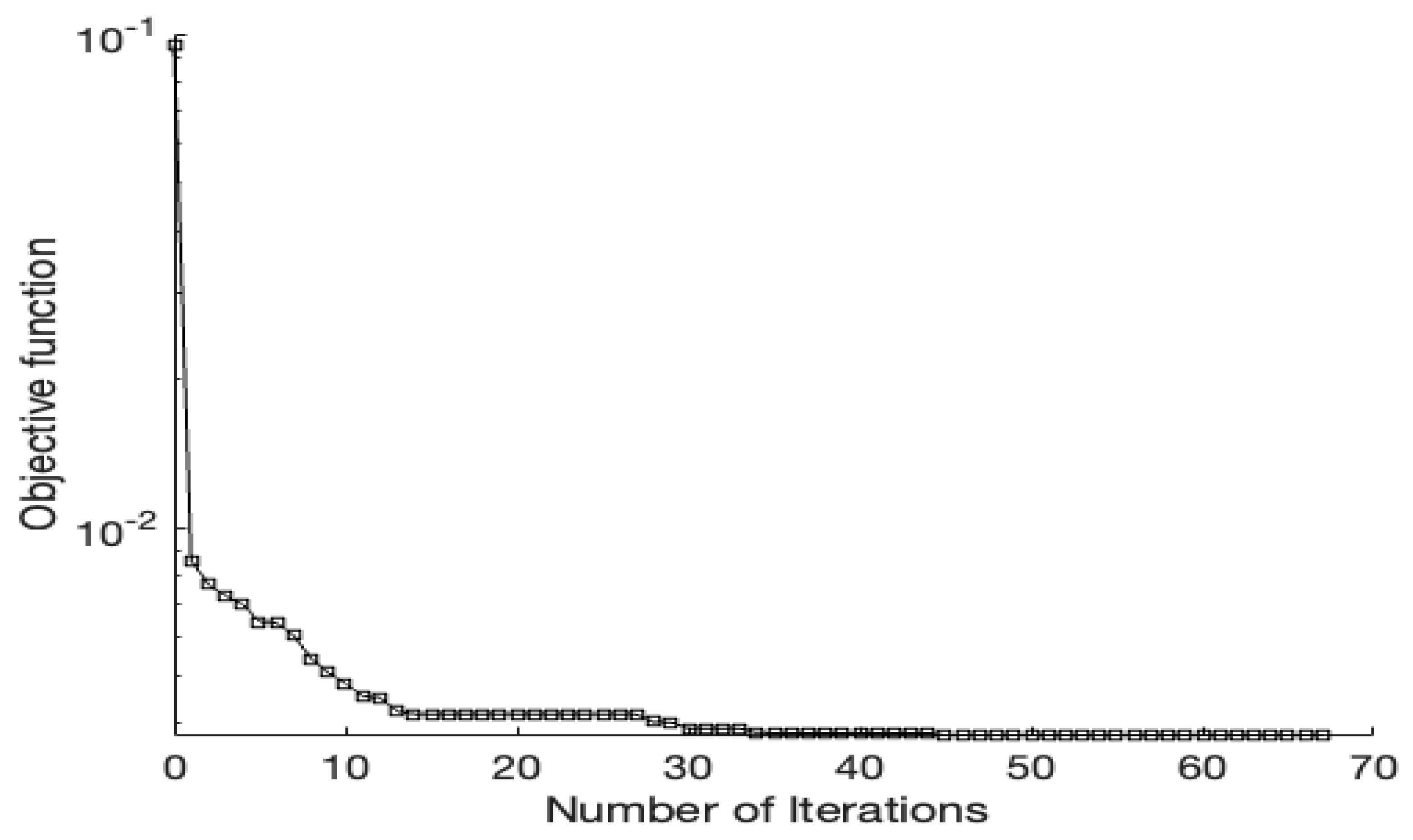
The misfit function without regularization ($\mathsf{\vartheta }=0$) under 1% noise is shown in Figure 19, where the function rapidly declines and stationary values are achieved after 20 iterations. The stationary value is reached at $O \left({10}^{-2}\right)$. Figure 20 illustrates the effect of various regularization values ($\mathsf{\vartheta }\in \{{10}^{-6}, {10}^{-5},{10}^{-4}\}$), where large $\mathsf{\vartheta }$ values increase stability but decrease accuracy, whereas small $\mathsf{\vartheta }$ values do not provide sufficient stabilization. The objective function minimization converges at each selection for $\mathsf{\vartheta }$ and achieves the minimum value. Also, in this case, the L-curve criterion has failed to spot the optimal value of $\mathsf{\vartheta }$, and there are two potential reasons for this: the nonlinearity of the IP and the non-smoothness of the recovered term. Hence, we omit the plot of the L-curve.

Figure 21 shows that the function converges rapidly to smaller values (${10}^{-4}$ or less) in the case of lower noise ($p=0.1\%$).

Table 5. Computational information obtained from lsqnonlin routine output during minimization processes for Example 2. The noise contamination percentage $pϵ\{1\%,0.1\%\}$ is depicted in (5) via (41) with various regularization parameter values.

$\mathit{p}=1\%$	$\mathsf{\vartheta }={10}^{-7}$	$\mathsf{\vartheta }={10}^{-6}$	$\mathsf{\vartheta }={10}^{-5}$	$\mathsf{\vartheta }={10}^{-4}$	$\mathsf{\vartheta }={10}^{-3}$	$\mathsf{\vartheta }={10}^{-2}$	$\mathsf{\vartheta }={10}^{-1}$
Count of iterations	67	27	6	9	4	20	17
No. of function evaluations	4216	1736	434	1240	310	1302	1116
Objective function	0.00378	0.00732	0.00784	0.00877	0.0118	0.03318	0.10947
$rmse\left(a\right)$	58.4103	2.1327	0.6205	0.2911	0.2045	0.2102	0.2489
Computational time (second)	199.64	190.68	48.39	133.009	34.202	148.127	120.74
$\mathit{p}=0.1\%$	$\mathsf{\vartheta }{=10}^{-7}$	$\mathsf{\vartheta }{=10}^{-6}$	$\mathsf{\vartheta }={10}^{-5}$	$\mathsf{\vartheta }={10}^{-4}$	$\mathsf{\vartheta }={10}^{-3}$	$\mathsf{\vartheta }={10}^{-2}$	$\mathsf{\vartheta }={10}^{-1}$
Count of iterations	9	6	5	21	15	20	15
No. of final evaluations	620	434	372	1364	992	1302	992
Objective function	6.50 $\times {10}^{-5}$	7.73 $\times {10}^{-5}$	0.000115	0.00040	0.00294	0.0241	0.1006
$rmse\left(a\right)$	0.9075	0.2470	0.1620	0.1859	0.2041	0.2105	0.2489
Computational time (seconds)	69.127	51.162	42.560	149.32	121.101	141.96	112.6

presents some numerical information, with the smallest rmse($a$) exhibiting the best retrieval. Figure 22 reveals that the best regularization value according to the L-curve method is located at corner of the L-shaped curve, and this value is $\vartheta \in [{10}^{-4},{10}^{-3}]$. As demonstrated in Example 1, the transverse displacement profile was not affected by the inclusion of noise, as plotted in Figure 23.

6. Conclusions

A numerical solution was obtained for inverse forced vibrations of a cantilever beam. Our aim was to find the transverse displacement $\mathcal{w}(\chi ,\tau )$ and time-dependent potential coefficient $a\left(\tau \right)$ in a fourth-order hyperbolic equation derived from supplementary measurements. The direct issue was discretized via the Crank–Nicolson FDM. To overcome the inherent ill-posed nature of the IP—which lacks continuous dependence on the input data—the Tikhonov regularization/stabilization approach was applied to provide the necessary stabilization. The inverse issue is resolved by the stabilization provided by the Tikhonov regularization approach.

• Consistent and accurate estimates for the time-dependent coefficient $a\left(\tau \right)$ were successfully reconstructed.
• The regularization method proved robust and effective for $\vartheta$ ∈ {${10}^{-5}$, ${10}^{-7}$}.
• The accuracy of the retrievals was maintained even in the presence of noise, and was specifically validated at noise levels of $p\%$ $\in \{1\%,0.1\%\}$.
• The proposed numerical solution and stabilization method performed reliably across smooth and non-smooth tests.

We have not attempted to extend our work to include multi-dimensional problems or more complex conditions; this will be addressed in future studies, since further theoretical and numerical investigation is needed.

References

1. Ricardo, H.J. A Modern Introduction to Differential Equations; Academic Press: Cambridge, MA, USA, 2020. [Google Scholar]
2. Narayanan, S.; Manicavachagom Pillay, T.K.; Ramanaiah, G. Advanced Mathematics for Engineering Students; S. Viswanathan Publisher: Chennai, India, 1993. [Google Scholar]
3. Kirkwood, J. Mathematical Physics with Partial Differential Equations; Academic Press: Cambridge, MA, USA, 2018. [Google Scholar]
4. Leung, A.W. Systems of Nonlinear Partial Differential Equations: Applications to Biology and Engineering; Springer: Dordrecht, The Netherland, 2013; Volume 49. [Google Scholar]
5. Zolotarev, V.A. Direct and inverse problems for a periodic problem with non-local potential. J. Differ. Equ. 2021, 270, 1–23. [Google Scholar] [CrossRef]
6. Favini, A.; Lorenzi, A. Differential Equations: Inverse and Direct Problems; CRC Press: Boca Raton, FL, USA, 2006. [Google Scholar]
7. Lesnic, D. Inverse Problems with Applications in Science and Engineering; Chapman and Hall/CRC: Boca Raton, FL, USA, 2021. [Google Scholar]
8. Wang, Y.; Yang, C. Inverse problems, optimization and regularization: A multi-disciplinary subject. In Optimization and Regularization for Computational Inverse Problems and Applications; Springer: Berlin/Heidelberg, Germany, 2011; pp. 3–14. [Google Scholar]
9. Lorenzi, A.; Paparoni, E. Identification problems for pseudohyperbolic integrodifferential operator equations. J. Inverse Ill-Posed Probl. 1997, 5, 523–548. [Google Scholar] [CrossRef]
10. Huntul, M.J.; Abbas, M. An inverse problem of fourth-order partial differential equation with nonlocal integral condition. Adv. Contin. Discret. Models 2022, 1, 55. [Google Scholar]
11. Cannon, J.R.; Dunninger, D.R. Determination of an unknown forcing function in a hyperbolic equation from overspecified data. Ann. Mat. Pura Appl. 1970, 85, 49–62. [Google Scholar] [CrossRef]
12. Tikhonov, A.N. On the stability of inverse problems. Dokl. Akad. Nauk SSSR 1943, 39, 195–198. [Google Scholar]
13. Ivanov, V.K. On linear problems which are not well-posed. Dokl. Akad. Nauk SSSR 1962, 145, 270–272. [Google Scholar]
14. Lavrentiev, M.M.; Romanov, V.G.; Vasiliev, V.G. Multidimensional Inverse Problems for Differential Equations; Lecture Notes in Mathematics; Springer: Berlin/Heidelberg, Germany, 1970. [Google Scholar]
15. Qahtan, J.A.; Hussein, M.S. Numerical solution to inverse coefficient problem for hyperbolic equation under overspecified condition of general integral type. AIP Conf. Proc. 2024, 2922, 090003. [Google Scholar] [CrossRef]
16. Hussein, S.O.; Lesnic, D.; Yamamoto, M. Reconstruction of space-dependent potential and/or damping coefficients in the wave equation. Comput. Math. Appl. 2017, 74, 1435–1454. [Google Scholar] [CrossRef]
17. Hussein, S.O.; Dyhoum, T.E. Solutions for non-homogeneous wave equations subject to unusual and Neumann boundary conditions. Appl. Math. Comput. 2022, 430, 127285. [Google Scholar] [CrossRef]
18. Megraliev, Y.T.; Alizade, F.K. Inverse boundary value problem for a Boussinesq type equation of fourth order with nonlocal time integral conditions of the second kind. Vestn. Udmurt. Univ. Mat. Mekh. Komp’yut. Nauki 2016, 26, 503–514. [Google Scholar] [CrossRef]
19. Bellassoued, M.; Aïcha, I.B. An inverse problem of finding two time-dependent coefficients in second order hyperbolic equations from Dirichlet to Neumann map. J. Math. Anal. Appl. 2019, 475, 1658–1684. [Google Scholar] [CrossRef]
20. Tekin, I. Determination of a time-dependent coefficient in a wave equation with unusual boundary condition. Filomat 2019, 33, 2653–2665. [Google Scholar] [CrossRef]
21. Stampka, K.; Sarradj, E. A time-domain finite-difference method for bending waves on infinite beams on an elastic foundation. Acoustics 2022, 4, 867–884. [Google Scholar] [CrossRef]
22. Durdiev, U.D.; Durdiev, D.D. Inverse problem of determining the time–dependent beam stiffness coefficient in the beam vibration equation using the finite difference method. Eurasian J. Math. Comput. Appl. 2024, 12, 41–56. [Google Scholar] [CrossRef]
23. Maciag, A.; Pawinska, A. Solving direct and inverse problems of plate vibration by using the Trefftz functions. J. Theor. Appl. Mech. 2013, 51, 543–552. [Google Scholar]
24. Karchevsky, A.L. Analytical Solutions to the Differential Equation of Transverse Vibrations of a Piecewise Homogeneous Beam in the Frequency Domain for the Boundary Conditions of Various Types. J. Appl. Ind. Math. 2020, 14, 648–665. [Google Scholar] [CrossRef]
25. Elvin, A. Inverse coefficient identification problem for a hyperbolic equation with nonlocal integral condition. Turk. J. Math. 2022, 46, 1243–1255. [Google Scholar] [CrossRef]
26. Bakushinsky, A.B.; Leonov, A.S. Fast numerical method of solving 3D coefficient inverse problem for wave equation with integral data. J. Inverse Ill-Posed Probl. 2018, 26, 477–492. [Google Scholar]
27. Markov, I.; Igumnov, L. Comparison of two numerical inverse Laplace transform methods with application for problem of surface waves propagation in an anisotropic elastic half-space. In Advanced Materials, Proceedings of the International Conference on “Physics and Mechanics of New Materials and Their Applications”, PHENMA 2019, Hanoi, Vietnam, 7–10 November 2019; Springer: Cham, Switzerland, 2020; pp. 353–368. [Google Scholar]
28. Hussein, S.O.; Hussein, M.S. Splitting the one-dimensional wave equation. Part II: Additional data are given by an end displacement measurement. Iraqi J. Sci. 2021, 62, 233–239. [Google Scholar] [CrossRef]
29. Hussein, S.O. Inverse one-dimensional wave equation problem under upper-base as additional information. Ital. J. Pure Appl. Math. 2022, 47, 596–608. [Google Scholar]
30. Mehraliyev, Y.T.; Huseynova, A.F. On solvability of an inverse boundary value problem for pseudo-hyperbolic equation of the fourth order. J. Math. Res. 2015, 7, 101–109. [Google Scholar] [CrossRef]
31. Ramazanova, A.; Mehraliyev, Y. On solvability of inverse problem for one equation of fourth order. Turk. J. Math. 2020, 44, 611–621. [Google Scholar] [CrossRef]
32. Rayleigh, L. Teoriia Zvuka (The Theory of Sound); Gostehizdat: Moscow, Russia, 1955. (In Russian) [Google Scholar]
33. Timoshenko, S.; Young, D.H.; Weaver, W. Vibration Problems in Engineering; John Wiley& Sons. Inc.: New York, NY, USA, 1974. [Google Scholar]
34. Taghiyev, R.M.; Farajova, S.S.; Ramazonova, A.T.; Allahverdiyev, R.N.; Shalimov, M.Y. Inverse Boundary Problem for the Equation of Forced Vibrations of a Cantilever Beam with Integral Conditions. Adv. Math. Sci. J. 2024, 13, 85–96. [Google Scholar] [CrossRef]
35. Mathworks: Documentation Optimization Toolbox—Least Squares Algorithms. 2019. Available online: www.mathworks.com (accessed on 1 June 2026).
36. Smith, G.D. Numerical Solution of Partial Differential Equations: Finite Difference Methods, 3rd ed.; Clarendon Press: Oxford, UK, 1985. [Google Scholar]
37. Gani, S.; Hussein, M.S. A fourth Order Pseudo parabolic Inverse Problem to Identify the Time Dependent Potential Term from Extra Condition. Iraqi J. Sci. 2024, 65, 4529–4549. [Google Scholar] [CrossRef]
38. Vichnevetsky, R. Stability charts in the numerical approximation of partial differential equations: A review. Math. Comput. Simul. 1979, 21, 170–177. [Google Scholar] [CrossRef]
39. Morozov, V.A. On the solution of functional equations by the method of regularization. Sov. Math. Dokl. 1966, 7, 414–417. [Google Scholar] [CrossRef]
40. Engl, H.W.; Hanke, M.; Neubauer, A. Regularization of Inverse Problems; Springer: Berlin/Heidelberg, Germany, 1996. [Google Scholar]
41. Gockenbach, M.S. Linear Inverse Problems and Tikhonov Regularization; American Mathematical Society: Providence, RI, USA, 2016. [Google Scholar]
42. Hansen, P.C. The L-Curve and Its Use in the Numerical Treatment of Inverse Problems. Available online: https://www.sintef.no/globalassets/project/evitameeting/2005/lcurve.pdf (accessed on 1 June 2026).
43. Hansen, P.C.; O’Leary, D.P. The use of the L-curve in the regularization of discrete ill-posed problems. SIAM J. Sci. Comput. 1993, 14, 1487–1503. [Google Scholar] [CrossRef]
Figure 1. Precise and estimated solutions for the transverse displacement w ( χ ,   τ ) , together with the absolute error with the grid size M = N = 60.
Mca 31 00132 g001
Figure 2. The exact solution and computational curve for desired output w 0 ,   τ .
Mca 31 00132 g002
Figure 3. Accurate and numerical outcomes for the prospective term a τ when M = N = 10,20,40,60,80 for Example 1.
Mca 31 00132 g003
Figure 4. The objective function (40) without regularized ϑ = 0 , and p = 0 noise mesh sizes M = N = { 10,20,40,60,80 } for Example 1.
Mca 31 00132 g004
Figure 5. Accurate and numerical results for the smooth potential term a τ without regularization, i.e., ϑ = 0 , and p = 1 % noise for Example 1.
Mca 31 00132 g005
Figure 6. The objective function (40) without regularized ϑ = 0 and p = 1 % noise for Example 1.
Mca 31 00132 g006
Figure 7. Accurate and numerical results for the smooth potential term a τ with regularized ϑ { 10 6 ,   10 5 , 10 4 } and p = 1 % noise for Example 1.
Mca 31 00132 g007
Figure 8. The objective function (40) with regularization parameters ϑ { 10 6 ,   10 5 , 10 4 } and p = 1 % noise for Example 1.
Mca 31 00132 g008
Figure 9. The L-curve plot with various amounts of regularization when p = 1 % noise for Example 1.
Mca 31 00132 g009
Figure 10. Accurate and numerical results for the smooth potential term a τ with regularized ϑ { 10 9 ,   10 8 , 10 7 } and p = 0.1 % noise for Example 1.
Mca 31 00132 g010
Figure 11. The L-curve plot with various regularization when p = 0.1% noise for Example 1.
Mca 31 00132 g011
Figure 12. The minimized objective functional (40), with ϑ { 10 9 ,   10 8 , 10 7 } and p = 0.1 % noise amount percentage for Example 1.
Mca 31 00132 g012
Figure 13. Accurate and approximate solutions for the transverse displacement of the w χ ,   τ with (a) p = 1 %   ϑ = 10 5 , (b) p = 0.1 % and ϑ = 10 7 .
Mca 31 00132 g013
Figure 14. Accurate and approximate results for the non-smooth potential term a τ when M = N = 10,20,40,60,80 for Example 2.
Mca 31 00132 g014
Figure 15. The objective function (40), without regularized ϑ = 0 , and p = 0 noisefor Example 2 at various mesh sizes M = N = 10,20,40,60,80 .
Mca 31 00132 g015
Figure 16. Accurate and approximate results for the non-smooth potential term a τ without regularized ϑ = 0 , and p = 1 % noise for Example 2.
Mca 31 00132 g016
Figure 17. Accurate and approximate results for the non-smooth potential term a τ with regularized ϑ { 10 6 ,   10 5 , 10 4 } and p = 1 % noise for Example 2.
Mca 31 00132 g017
Figure 18. Accurate and approximate solution for the non-smooth potential term a τ with ϑ { 10 7 ,   10 6 , 10 5 } and p = 0.1 % noise for Example 2.
Mca 31 00132 g018
Figure 19. The misfit function (40), without regularized ϑ = 0 , and p = 1 % noise for Example 2.
Mca 31 00132 g019
Figure 20. The misfit function (40), with ϑ { 10 6 ,   10 5 , 10 4 } and 1 % noise amount contaminated in (5) via (41) for Example 2.
Mca 31 00132 g020
Figure 21. The regularized misfit function (40) with regularization parameter ϑ { 10 7 ,   10 6 , 10 5 } and p = 0.1 % noise contaminated in (5) via (41) for Example 2.
Mca 31 00132 g021
Figure 22. The L-curve plot with various levels of regularization when p = 0.1 % noise for Example 2.
Mca 31 00132 g022
Figure 23. Accurate and approximate solutions for the transverse displacement of the w χ , τ with (a) p = 1 % and ϑ = 10 3 , (b) p = 0.1 % and ϑ = 10 4 .
Mca 31 00132 g023