


Abstract
Quantum computing has emerged as a revolutionary technology in recent years, with wide-ranging applications across many fields. It provides a significant advantage in terms of exponential speedups, leading researchers to believe that classical computing cannot overcome this gap. However, its true potential has not yet been thoroughly investigated in statistics. In the present study, we incorporate quantum dynamics into the statistical estimation method and propose a quantum-based estimation approach, i.e., quantum maximum likelihood estimation. The proposed method leverages quantum principles and dynamics to estimate the unknown parameters of probability distributions. This study implements the proposed method to estimate the Laplace location parameter. Simulation studies and real-world analyses are performed to evaluate the performance of the QMLE estimate of the Laplace parameter compared to the MLE estimate. The validity of the QMLE estimate is also assessed through variance and convergence analyses. All the findings validate the potential computational advantages of the QMLE approach as a competitive and promising method for parameter estimation of the Laplace parameter. QMLE provides more accurate, precise, efficient, less uncertain, and better-fitting estimates than MLE. Overall, the results indicate that statistical estimation theory can be improved by incorporating quantum dynamics into the classical estimation process.
1. Laplace Distribution
Pierre-Simon Laplace introduced the Laplace distribution, also called the first law of Laplace, in 1774. The second law of Laplace, also called the Gaussian or normal distribution, was proposed in 1778. The random variable of the Laplace distribution arises as the difference of two exponential variables with the same scale, so it is also known as the double exponential distribution.
The exponential decay in the density function of the Laplace distribution, measured by the absolute distance from the mean, leads to slower decay in the tails and a higher central peak. Therefore, the Laplace distribution has a sharper peak and heavier tails than the normal distribution, indicating it is leptokurtic. The simplicity of Laplace distributions and their characteristic functions make them popular in probability theory. Laplace distributions were used by the famous probabilist J.M. Keynes in 1911 as a law of errors. This distribution has a broader range of applications in various fields, including engineering, business, biology, astronomy, environmental sciences [1], life testing, machine learning, finance, economics, speech and image recognition, quality control, hydrology, geology, telecommunication, and nuclear medicine. The probability density function of the classical Laplace distribution, with location and scale parameters, has the following form.
Here, represents the location parameter and represents the scale parameter of the Laplace distribution. It is a symmetric distribution around , whose tails are heavier than normal distribution but not heavier than those of a Cauchy distribution. The Laplace distribution has close relationships with other distributions, such as exponential, chi-square, uniform, Cauchy, normal, Rayleigh, and double Lomax distributions. Its role in the theory of Brownian motion for modeling random times is also significant. It highlights the importance of the Laplace distribution in distribution theory [2]. The Laplace distribution models symmetric data with long tails, while the normal distribution is used when the tails are shorter. This characteristic enables the Laplace distribution to model data with extreme values (outliers) more effectively. It is essential to choose an appropriate probability distribution in statistical inference, with tail probabilities, to draw the best possible conclusions [3,4]. The Laplace distribution is also used for error modelling, e.g., in global navigation systems, astronomy, etc., which motivates the least absolute deviation method for parameter estimation [5].
Many studies introduced skewness into symmetric distributions and proposed their skewed forms. Various skewed forms of the Laplace distribution have also been introduced in the literature. One of the earliest skewed forms of Laplace has the probability density function as
where [6].
Moreover, various studies have proposed generalized and extended forms of the Laplace distribution to capture heavy-tailed probabilities. Further research continues to highlight its key role and to reflect more real-world applications of the Laplace distribution in life testing, reliability, telecommunications, and related fields.
2. Methods of Estimation
Methods of statistical analysis heavily depend on the underlying probability distributions. To model the various phenomena of the real world, larger classes of probability distributions and statistical methodologies have been developed over the years. Further, the parameter estimation of these probability distributions plays a significant role in statistical inference. It provides the fundamentals for prediction, modeling, and decision making across several real-life domains [3]. The Laplace distribution is an important distribution for modeling lifetimes in telecommunications, engineering, and life testing. It is often used as an alternative distribution of the Gaussian distribution in some robustness studies. The location parameter represents the mean of the Laplace distribution, while the scale parameter controls its spread. Accurate parameter estimation for the Laplace distribution is crucial in environmental and biological sciences, astronomy, life testing, medicine, inventory management, finance, and quality control [6].
Several statistical methods, with distinct characteristics and tailored to specific real-world scenarios, are proposed for parameter estimation. Maximum likelihood estimation (MLE), method of moments (MoM) [3,7,8], and Bayesian methods are among the most widely used for estimating the parameters of the Laplace distribution. Linear estimation based on ordered observations and best linear unbiased estimators is also found in the literature for Laplace parameters [4,9]. Further, methods such as L-moments [10], trimmed L-moments [11], and robust estimation [12] have also been proposed for parameter estimation of probability distributions. Recently, a method called quantile least square has also been used for the estimation of location-scale families [13]. However, these methods are computationally intensive and are not widely used for parameter estimation of the Laplace distribution.
One of the powerful statistical estimation methods is MLE, which estimates the parameters of different probability distributions using observed data. MLE maximizes the likelihood function , of a probability distribution and identify the parameter’s value which maximizes . Here represent the values of observed data and represents the parameter [14,15]. MLE estimates are invariant, sufficient, asymptotically efficient, and consistent estimates. These estimates are asymptotically unbiased but biased in small samples. Additionally, these estimates are numerically sensitive to small changes in observed values and become inconsistent when the model is not specified correctly [16,17]. Moment estimates are biased, less efficient, inconsistent, and do not offer a natural framework for handling censored data and variance estimation [16]. The location parameter of the Laplace distribution is the median when its likelihood function is maximized [3], whereas its moment estimate is the mean [7].
The method of Bayesian estimation involves prior and posterior distributions, and the choice of prior information is crucial. All the inferences are based on the selection of previous knowledge. Bayesian estimation can yield computationally intensive and biased results with non-conjugate priors [18]. A prior distribution provides prior knowledge about the parameters, while the posterior distribution for Bayesian estimation is obtained from the likelihood of the sample distribution and this prior distribution [15]. Researchers used various discrete and continuous probability distributions and loss functions as prior information for Bayesian estimation of Laplace parameters [4,9,19].
Accurate and precise parameter estimation validates theoretical foundations and enables sound decision making and predictive modeling in statistical inference. The most common methods for estimating Laplace parameters across various applied fields are the MOM, MLE, and Bayesian methods. Notwithstanding the significant success of these estimation methods, they have pros and cons depending on the specific application, data nature, sample size, and inferential objectives, offering trade-offs among efficiency, accuracy, robustness, and interpretability. Further, in cases of censored samples or sparse data where precise measurements are difficult, implementing these methods becomes challenging. These limitations motivate the adoption of novel computational technologies, such as quantum computing (QC), in statistical estimation procedures. QC uses principles of quantum mechanics to speed up computation by allowing parallel paths. The development of quantum-based statistical estimation, such as quantum maximum likelihood estimation, can accelerate the estimation process potentially, improving the precision and accuracy of classical methods.
3. Quantum Computing
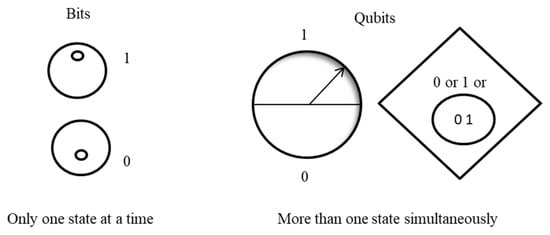
Classical computing achieved tremendous success in the 1950s due to its high computational power. However, the potential of quantum computing to solve complex tasks more efficiently attracted scientists, and by the 1980s, they began to consider this new computing paradigm. QC has emerged as a revolutionary technology in recent years due to its widespread applications across various fields. Its mechanical system performs computations on quantum hardware using principles of quantum mechanics, such as quantum superposition, interference, and entanglement. The significant speed advantage of QC over classical computing indicates its supremacy, and researchers strongly believe that classical computing cannot overcome this gap [20]. Quantum computations use qubits, or quantum bits, to process quantum information, while classical computation relies on bits and has a limited ability to perform complex calculations. There are only two possible values for bits: 1 or 0, which describe their state as having only one value at a time. At the same time, a qubit not only exists in its pure states of 0 or 1 but also in a linear combination of these pure states at the same time, i.e., in more than a single state simultaneously, known as a superposition. The generic states of bits and qubits are shown in Figure 1 [21].
Figure 1.
Generic states of classical bits and qubits.
Dirac notation is a standard notation used to represent quantum states in quantum mechanics. For instance, Dirac ket vectors of two pure states or have their respective complex matrices and . The superposition state of qubits as a linear combination of pure states is defined as
where the coefficients and belong to complex numbers such that , representing the probability amplitude of two basic states, i.e., . Qubits are used to store information in a quantum mechanism, where superposition and entanglement play significant roles [20]. Superposition enables quantum parallelism in QC, enabling vast calculations to be conducted simultaneously. It reduces the number of computational steps and solves high-complexity problems more efficiently. Its combination with entanglement enables parallel computation and improves computational efficiency, enabling probabilistic solutions in quantum algorithms [22]. Quantum entanglement indicates the relationship between several qubits when they are combined and correlated. It enables information to propagate between distant quantum systems and allows a single qubit to change the overall state of all other qubits when an operation is performed on it. This characteristic increases computational efficiency [23]. Another property of QC is quantum coherence, which enables quantum states to maintain their superposition state over time despite external interference. Qubits are initialized in a register to process the QC and store information in a quantum processor, where quantum gates are applied to these input qubits. Quantum entanglement and superposition enable quantum gates to change the state of qubits and perform computations to generate some classical output. Qubit initialization is important for processing quantum information and for performing quantum computation [20,24]. Qubits, their quantum states, quantum gates, and quantum circuits are building blocks of quantum computing in quantum algorithms.
Current developments in quantum-based methodologies across various fields motivate academic researchers and statisticians to incorporate quantum dynamics into statistical methods. This incorporation will bridge the gap between quantum computing and statistics. Given the significant use of the Laplace distribution across various domains, the growing demand for computing, and the growing strength of quantum computing, this study proposes a quantum-inspired estimation framework to estimate the parameters of the Laplace distribution. This approach has the potential to outperform the classical estimation approach and improve the statistical estimation process.
4. Quantum Maximum Likelihood Estimation
Maximum likelihood estimation is a classical estimation method that uses observed data and obtains parameter estimates by maximizing the likelihood function of the probability distributions. MLE provides invariant, sufficient, asymptotically efficient, and consistent estimates. However, its estimates are numerically sensitive, biased and have some computational limitations for complex models and high-dimensional data [17]. Richer dynamics of QC offer the computational efficacy to cope with these challenges, providing potential advantages. Many researchers have attempted to incorporate quantum evolution into classical estimation methods to estimate quantum parameters [25,26,27,28]. Recently, Clausen et al. [25] used the Kraus map, sensitivity equations, quantum filter, and stochastic differential equations to formulate a recursive log-likelihood gradient framework and estimated quantum parameters [25]. The Kraus map is a mathematical tool that describes the changes in quantum states due to the measurement process or environmental interactions [20]. A quantum filter is another tool that mathematically estimates the evolution of quantum states over time. In practice, it is not easy to observe a true quantum state due to measurement disturbance and quantum uncertainty [29]. Surace and Pfister [27] also used quantum states, a quantum filter, and its corresponding sensitivity equations to estimate quantum parameters via MLE. However, Cortez et al. [26] did not involve the propagation of the quantum filter in their computations.
In the present study, we incorporate quantum dynamics into the statistical estimation method, and a quantum-based estimation approach, i.e., quantum maximum likelihood estimation (QMLE), is proposed. The proposed QMLE method leverages quantum principles via the Kraus map, quantum states, sensitivity equations, and a quantum filter to estimate the unknown parameters of probability distributions. Further, this study implemented the QMLE method to estimate the Laplace parameters. The Kraus map, quantum state, and quantum filter play a significant role in the quantum-inspired estimation approach. The Kraus map determines the quantum state evolution under decoherence and measurements, while the quantum filter updates these states. Further, the gradient-ascent-based approach iteratively estimates the unknown parameters in this QMLE method.
This proposed framework aims to provide more accurate and efficient parameter estimates for continuous probability distributions to improve statistical estimation by integrating quantum theory into the classical estimation method. The performance of this novel QMLE framework will be compared with that of the classical MLE method. The classical MLE method serves as a widely used and standard benchmark in statistical inference. The direct comparison between QMLE and MLE aims to evaluate the potential advantages of quantum incorporation into classical estimation procedures and assess whether the quantum-inspired framework provides any improvements compared to classical likelihood estimation. The QMLE approach has the potential to outperform the classical MLE method. Laplace distribution has closed form MLE estimates and well-understood properties. We used Laplace distribution as a benchmark problem in our study to evaluate the statistical performance, convergence behavior and feasibility of our proposed QMLE framework, estimating the same statistical objects as classical MLE. Our broader motivation is introducing a quantum-inspired estimation mechanism, which can be extended for the scenarios where the closed form estimators are not available.
4.1. QMLE Framework
We consider a density matrix to represent the mathematical form of quantum states. For a valid density matrix, it holds that i.e., is a complex matrix of size , and . These properties highlight the probabilistic nature of , encapsulating all statistical information of a quantum state. In our proposed QMLE framework, the quantum state evolves continuously under stochastic measurement outcomes, and the evolution determines each measurement outcome at each minor interval after the Kraus map is applied. The Kraus map in the current quantum state , depending on measurements and parameter , has a mathematical form
where
Equation (4), a stochastic master equation (SME), captures measurement effects and decoherence arising from measurement inefficiency. defines the quantum state evolution during a small time interval, i.e., , conditioned to stochastic measurement outcome . The measurement operator integrates both stochastic and deterministic dynamics and confirms the accurate mathematical form of quantum state evolution. models decoherence with , where indicates ideal measurement. Further, Hamiltonian operator specifying the unitary evolution subject to parameters ‘’ and Lindblad operator , models the decoherence induced by measurements, indicating an environmental effect on the quantum state. The Hamiltonian operator needs to hold ensuring unitary evolution, and must be a well-defined linear operator, reflecting measurement back-action and decoherence. In our QMLE framework, the selection of and is very important. in Equation (6) defines an incremental measurement signal of measurement outcomes, where the Wiener process is a noise in measurement outcomes which captures the probabilistic nature of measurement and is the expected value of with respect to . This equation indicates a balance between deterministic evolution of the quantum state and randomness.
In our QMLE methodology, Hamiltonian term updates the quantum state depending on the unknown value of parameter ‘’. Parameter ‘’ is estimated by maximizing , which is based on this quantum state evolution. A quantum filter is used to describe the evolution of the quantum state under decoherence and measurement (Equations (7) and (8)):
where , a probability of measurement outcome based on the parameter and quantum state. Trace ensures normalization of the updated density matrix, i.e., . As the true quantum state is unknown, we use , the best estimated quantum state, to obtain an estimate of the true ‘’.
Likelihood function over measurements conditioned on the initial estimated quantum state and parameter is defined as
It can be written as
The recursive form of this likelihood function and its log-likelihood function are given in Equations (15) and (16), respectively.
We take and :
Gradient Ascent Approach
Gradient ascent is the most commonly used approach in parameter estimation to maximize the log-likelihood function. It iteratively updates an estimate , starting from an initial guess , and steps in the direction of the gradient with , i.e., some varying step size. In our QMLE framework, Equation (19) provides an iterative update to maximize , where is the gradient of w.r.t. , computed at the current estimated value, which depends on and , a complete measurement record.
Equation (20) encapsulates both direct and indirect effects of on where the indirect effect is captured through the impact on at each time . This decomposition structure simplifies computations by separating the effects and aligns with quantum filtering, in which quantum state estimates are continuously updated. We used the sensitivity equation to capture the changes in due to and provide the computationally feasible formulation of the estimation process. We define , filter sensitivity at time , while is a filtered quantum state. Filter sensitivity measures the sensitivity of w.r.t. parameter . It is traceless, i.e., , a Hermitian operator having dimensions the same as those of . We differentiate given in Equation (9) w.r.t. to find filter sensitivity :
Equation (18) implies that
sums all the previous incremental contributions of log-likelihood from initial measurement to current measurement, i.e., . Instead of recalculating from scratch at each step, it enables incremental gradient updates with measurements.
implies
Also,
We obtain Equation (29) from Equations (26)–(28)
Equation (19) of updating a parameter estimate becomes
Equations of quantum filter (9–10), filter sensitivity (22), and gradient updates (30) provide our framework of the QMLE framework to estimate an unknown parameter .
The above framework will simulate all previous states and filter updates, i.e., the entire quantum trajectory, for gradient computation, which is computationally intensive. Instead of computing the gradient over the whole quantum trajectory, we can use the latest recursion of the quantum filter and the sensitivity equation to approximate it before updating the estimate. It emphasizes the latest modification in log-likelihood for the gradient computation and the preceding function becomes independent of and , once it has been used to estimate i.e., . It simplifies gradient computation. The QMLE trajectory is updated as
This framework updates the parameter estimates for each of the observation recursively in real time using incoming data, rather than recalculating it over the entire dataset. The final estimate of these update estimates is obtained by applying the estimation functional of the statistical model or probability distribution under consideration.
5. QMLE Framework for Estimating Laplace Parameter
The Laplace distribution is important in statistical inference due to its practical relevancy. Its location parameter represents the distribution’s mean, while its scale parameter controls the distribution’s spread. Accurate estimation of Laplace parameters is crucial for statistical modeling in environmental and biological sciences, life testing, astronomy, medicine, inventory management, finance, and quality control [6]. The QMLE parameter estimation method uses quantum filtering and its sensitivity equations to incorporate classical data into the quantum estimation trajectory and provides data-driven estimates. This section describes the implementation of the proposed QMLE framework to estimate the Laplace parameter. Primarily, our study focuses on estimating the location parameter of the Laplace distribution, assuming the scale parameter is known. The idea is implanting classical likelihood estimation into quantum dynamics, where stochastic evolution provides estimates. For this purpose, a Kraus map as a measurement operator encodes the Laplace parameters in a quantum system, incorporating both deterministic and stochastic effects and is given as
where and are Hamiltonian and Lindblad operators, respectively, defined as
The Hamiltonian and Lindblad operators are valid, aligned with the quantum trajectory for estimating the Laplace parameter using the QMLE framework, and chosen according to structural properties of Laplace likelihood. The Laplace distribution reflects the piecewise linear log-likelihood and heavy-tailed natures that distinguish it from a normal distribution. The Hamiltonian operator is constructed to capture this behavior depending on parameters where is the location parameter to be estimated and is a known scale parameter. It linearly depends on through that encodes as a phase shift in quantum state while incorporated through ensures quantum evolution under heavy-tailed noise. The Lindblad operator models an interaction between a quantum system and the environment through , and . The value of controls the strength of quantum measurement and defines estimation sensitivity, having a direct influence on the measurement outcomes and estimation process. It requires compatibility with quantum dynamics, i.e., a value that is neither too high nor too low. This stochastic dynamics of the Lindblad operator allows quantum filtering to generate gradient updates, being consistent with the Laplace score-function, and supports robust parameter estimation. The Hamiltonian operator introduces a unitary evolution and defines irreversibility, and both make it a real-world system. Additionally, and are the Pauli gates, which are used to model real quantum dynamics in this estimation framework. These gates acquire important information from the external environment and process parameter estimates. shows a measurement signal, which is affected by stochastic noise , Lindblad and , described as
The quantum filter evolves a quantum system, and updates the estimates of parameters based on the measurements, as
Further, an equation of filter sensitivity is obtained by differentiating the quantum filter given above w.r.t. parameter .
We obtain parameter updates for the estimation of an unknown parameter as
The dynamics of our proposed QMLE uses a quantum filter and evolution of quantum state to estimate the unknown parameters. This framework is consistent with classical estimation by MLE and provides quantum stochastic benefits, upholding the statistical structure of probability distributions.
The QMLE performance depends on several hyperparameters, i.e., measurement strength , learning rate , measurement efficiency , time step . These hyperparameters govern the learning process and quantum dynamics. The accuracy of the estimator depends on and its moderate value balances the noise and information gain. represents the measurement efficiency and its value closer to 1 improves the precision of the estimation and the performance of QMLE degrades as decreases. controls the step size in parameter updating. Its larger values lead to the fastest convergence but may also increase instability. However, an adaptive learning rate improves stability. controls the numerical resolution in quantum filter updating. A sufficiently smaller value of time step provides stable evolution of quantum state, ensuring more accurate and stable estimates. Further, a much smaller value of decay factor allows smooth step size reduction in optimization and improves the convergence robustness.
Quantum Algorithm
The QMLE framework for estimating the Laplace location parameter is summarized as an algorithm.
Step 1: Initialize various QMLE parameters such as , Pauli gates and , number of iterations = , decay factor = and adaptive learning rate = having and bounds .
Step 2: Define the initial value of the quantum state as , filter sensitivity as , and the initial mean estimates as .
Step 3: Iterate using Equations (35)–(39) times, update the equations of the quantum filter (40) and filter sensitivity (42), compute gradients and update estimates using Equation (43) after every iteration.
Step 4: Store these updated values of for each sample and compute the median of these stored values as a QMLE estimate of the location parameter of the Laplace distribution.
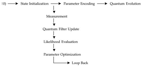
It uses one-qubit representation of quantum state where the measurement operations are performed at each of iteration and have unitary evolution. The representation of a single qubit is sufficient to encode the location parameter where two Pauli gates are applied to perform the evolution of quantum state. The measurement complexity of this algorithm is proportional to the number of simulation replications and number of iterations. To implement this algorithm practically and estimate the parameter accurately, we require multiple measurements at each of iteration. An end-to-end implementation of the quantum-inspired algorithm is given in a diagram representation below (see Figure 2).
Figure 2.
Quantum-inspired algorithm.
This study also evaluates the performance of the QMLE estimate of the Laplace parameter compared with its analytically computed MLE estimate in both simulation studies and real-world analyses. For this purpose, we compute various statistical metrics such as bias, mean absolute error (MAE), relative mean error (RME), root mean squared error (RMSE), mean squared error (MSE), coverage probabilities (CP), average length (AL) from 95% confidence interval, standard error (SE), and variance and convergence plots.
- Mean Square Error (MSE)
- Mean Absolute Error (MAE)
- Confidence Interval
The confidence intervals (95%) for both classical MLE and QMLE are constructed using SEs computed from the repeated Monte Carlo simulations. The empirical standard deviation of the estimates is computed across Monte Carlo runs for each of the estimators and used as SEs. The normal approximation is used to construct the confidence intervals as
where and represents Monte-Carlo-based standard deviation of the estimates. The AL is calculated by taking the mean width of constructed intervals across all runs while the CP is computed as proportion of simulation replications within which the intervals contain the true parameter.
6. Simulation Study
The simulation study estimates the Laplace location parameter using both classical MLE and QMLE methods and evaluates the accuracy and efficiency of QMLE estimates across numerous metrics. Its objective is to validate the theoretical advantage of incorporating quantum computations into classical statistical estimation and to assess the performance of the QMLE method compared to classical MLE. The classical method is used as a benchmark for comparison. In this section, we conduct the simulation studies based on 100 Monte Carlo (MC) runs, and data is generated from the Laplace distribution of size having different settings of true parameters and sample sizes (Table 1).
Table 1.
Simulation settings.
These combinations of parameters show location shifts from moderate–large–extreme while the scale parameters are capturing light–heavy-tailed noise. This aims to assess the robustness of estimators under varying signal and noise. Further, we set a different value of random seed for each run of the MC simulation such that
to maintain statistical independence across various configurations of parameters and reproduce the results. Classical MLE and QMLE estimates of the location parameter are computed for the same simulated data, where is computed by taking the sample median of each MC replication. The results for estimation of the Laplace location parameter and RMSE, CP and AL of 95% confidence intervals for these estimates are presented in Table 2. Moreover, the results of bias, MAE, RME, and MSE across runs are given in Table 3.
Table 2.
Comparative analysis of QMLE and MLE estimates of Laplace parameter across runs.
Table 3.
Empirical evidence for QMLE and MLE estimates over multiple runs (Mean ± S.D).
The results of simulation studies indicate that the QMLE approach is well-calibrated and provides a closer estimate of the true value of the Laplace parameter than the classical MLE method under these settings. Further, QMLE estimates are more accurate, efficient, and statistically significant than MLE estimates, providing reduced bias, lower error measures, and shorter length of confidence intervals in all simulation studies. Although both estimates yield higher values of coverage probabilities, short AL for QMLE estimates highlight that these estimate do not sacrifice the coverage and achieve higher inferential efficiency. These findings validate the practical advantage of QMLE over MLE.
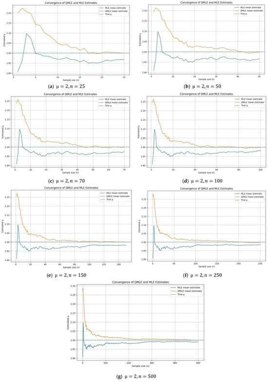
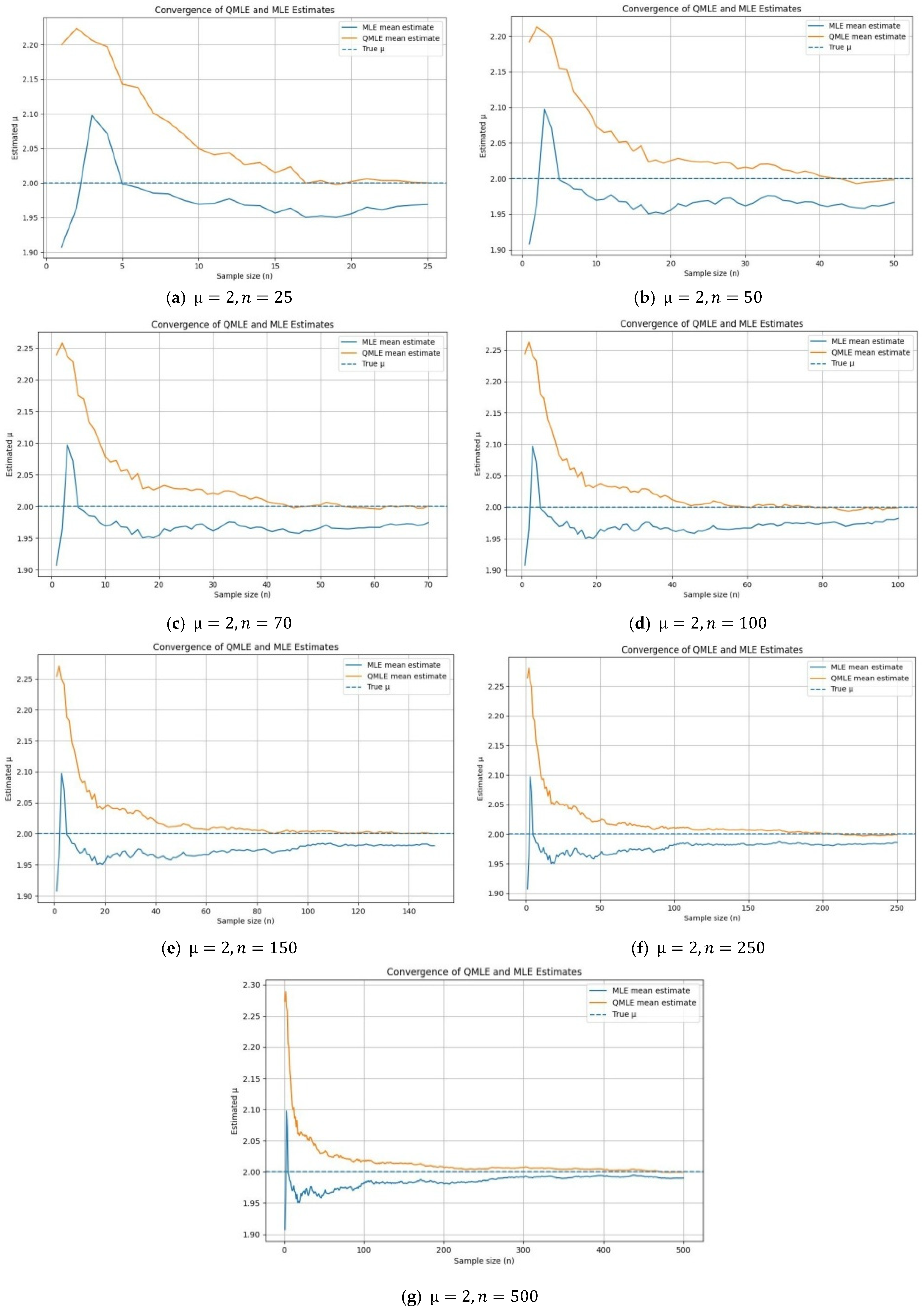
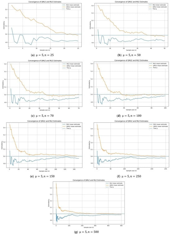
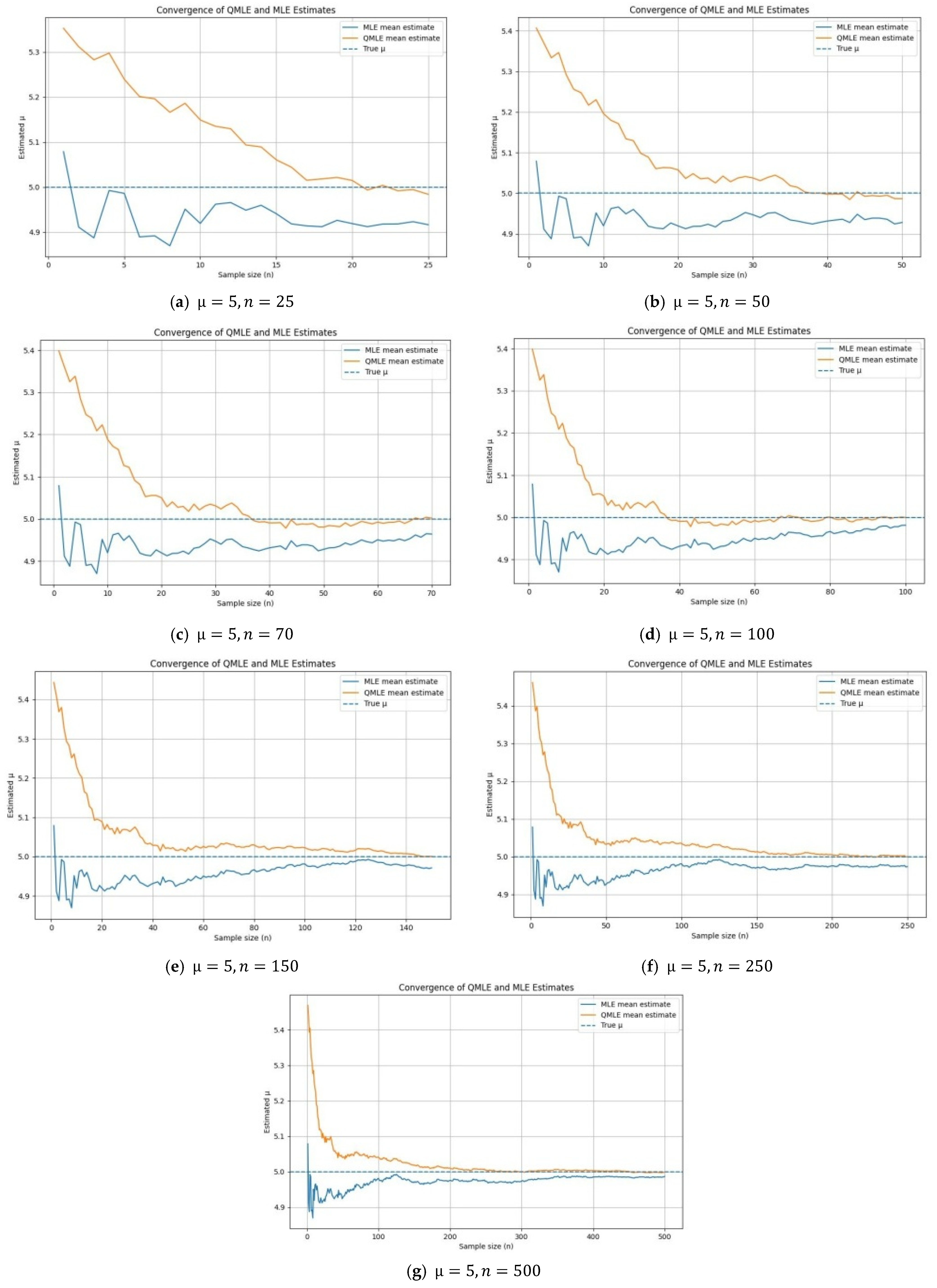
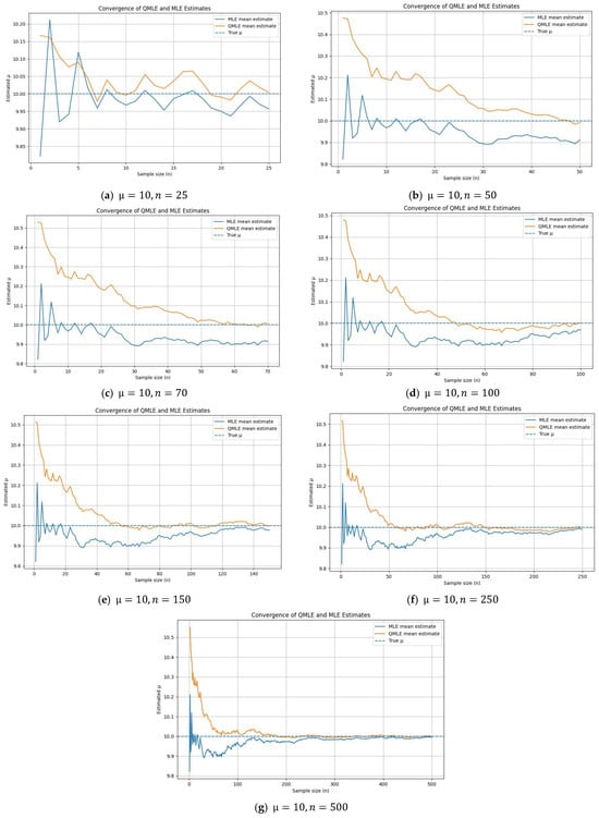
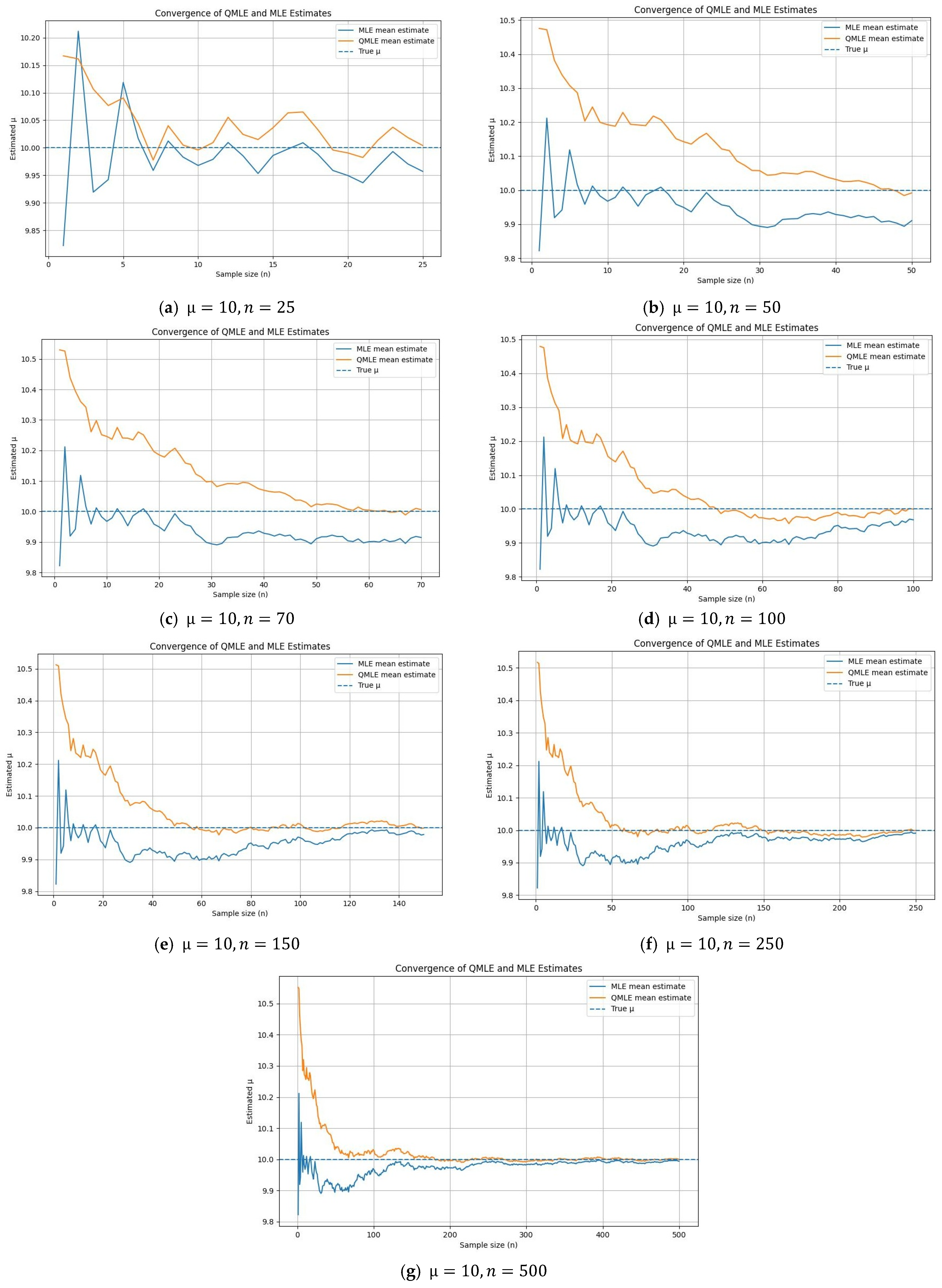
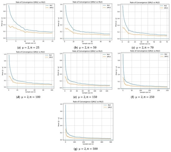
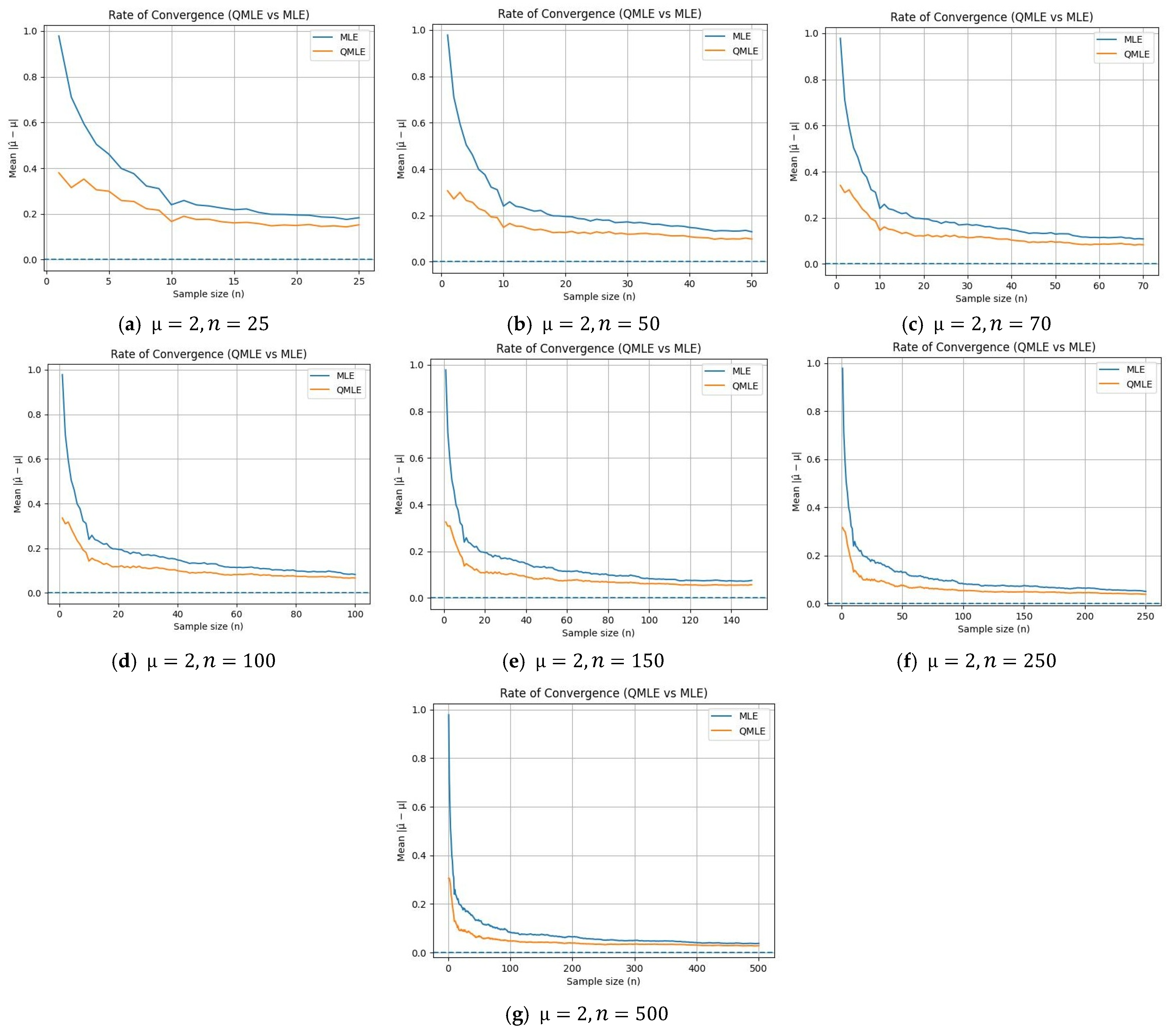
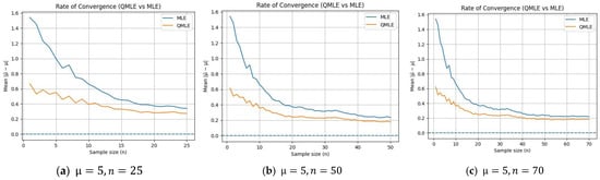
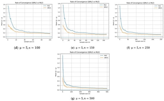
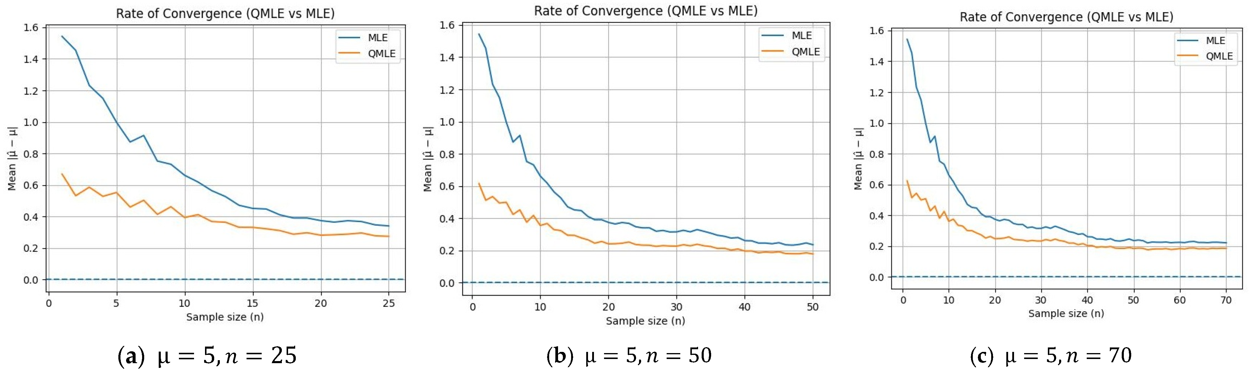
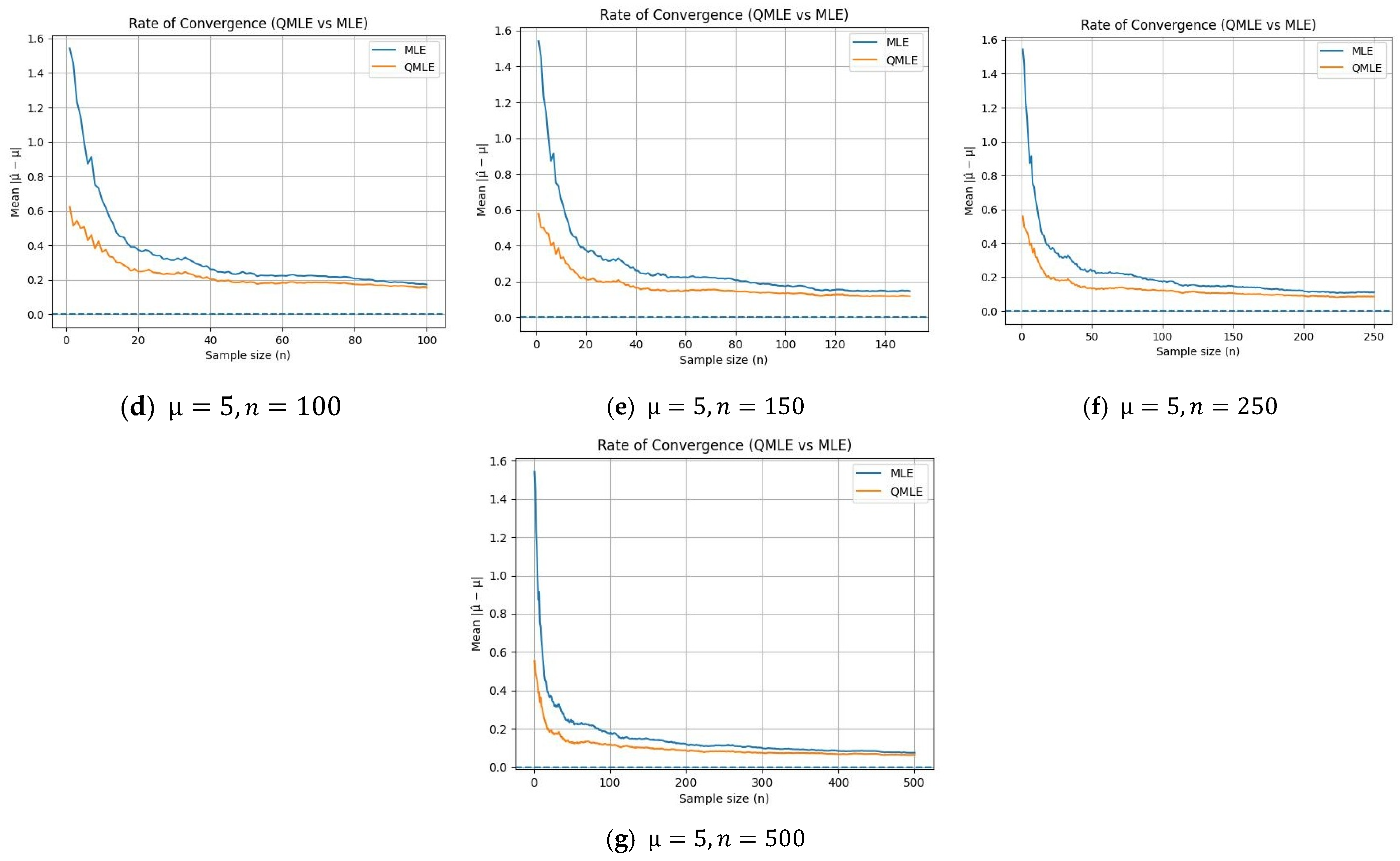
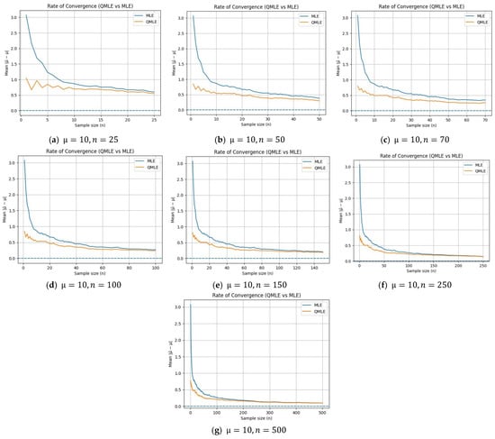
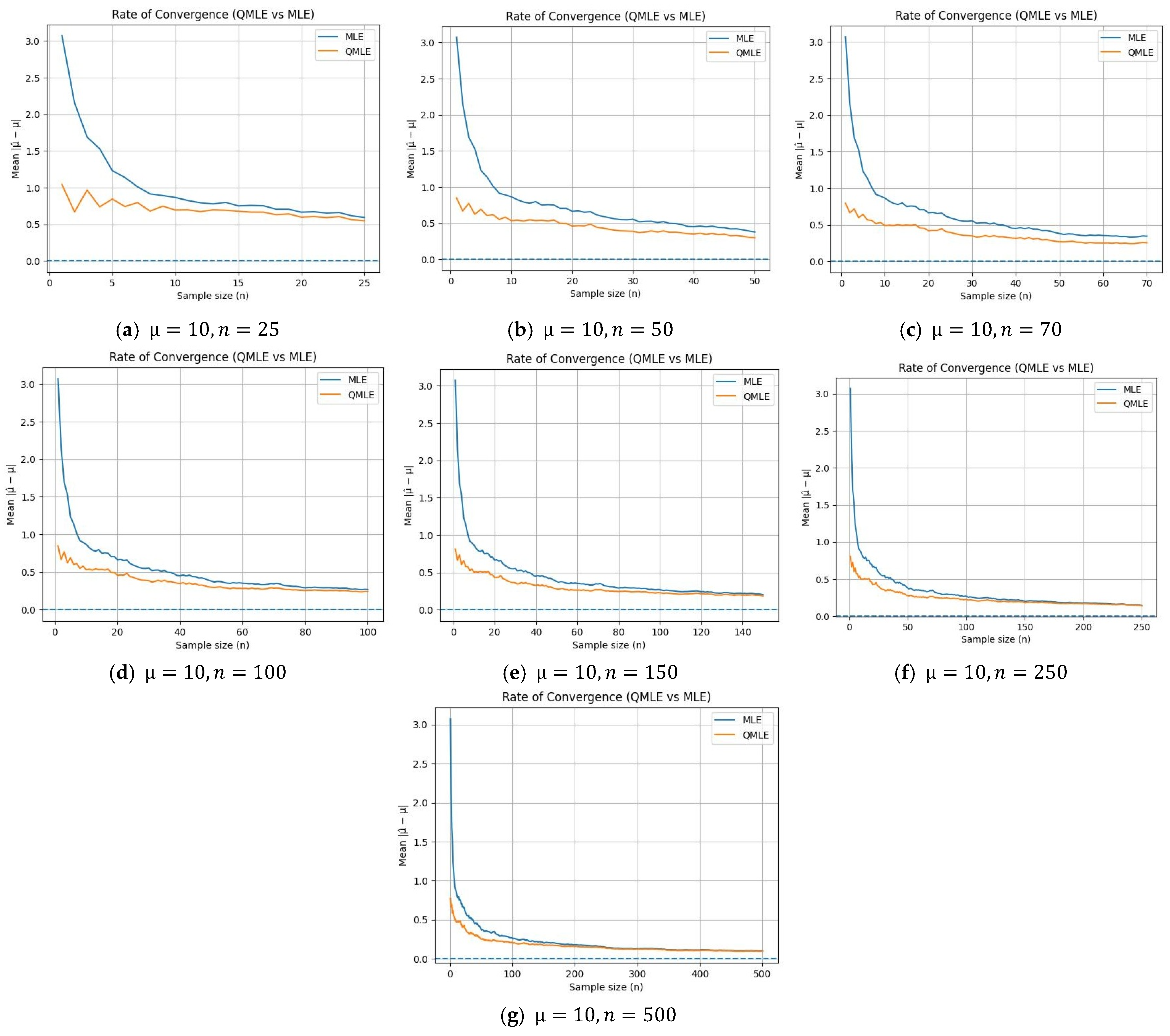
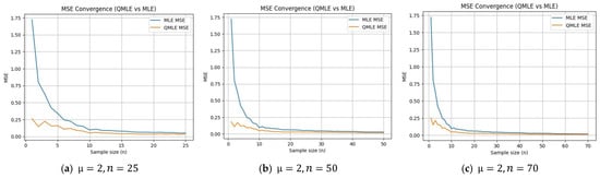
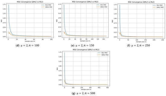
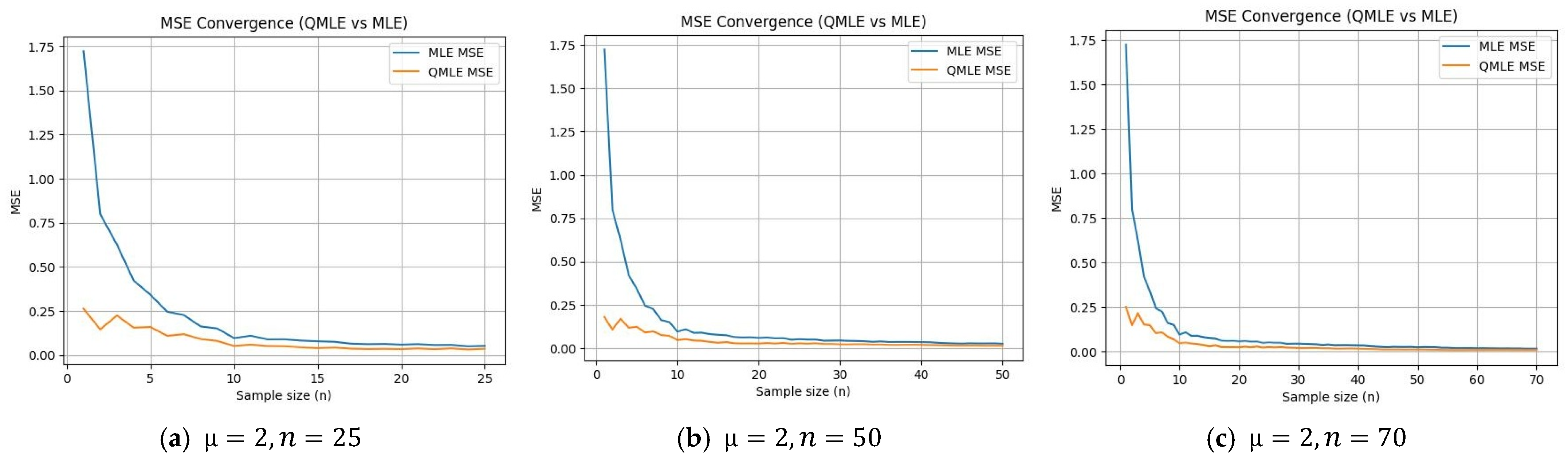
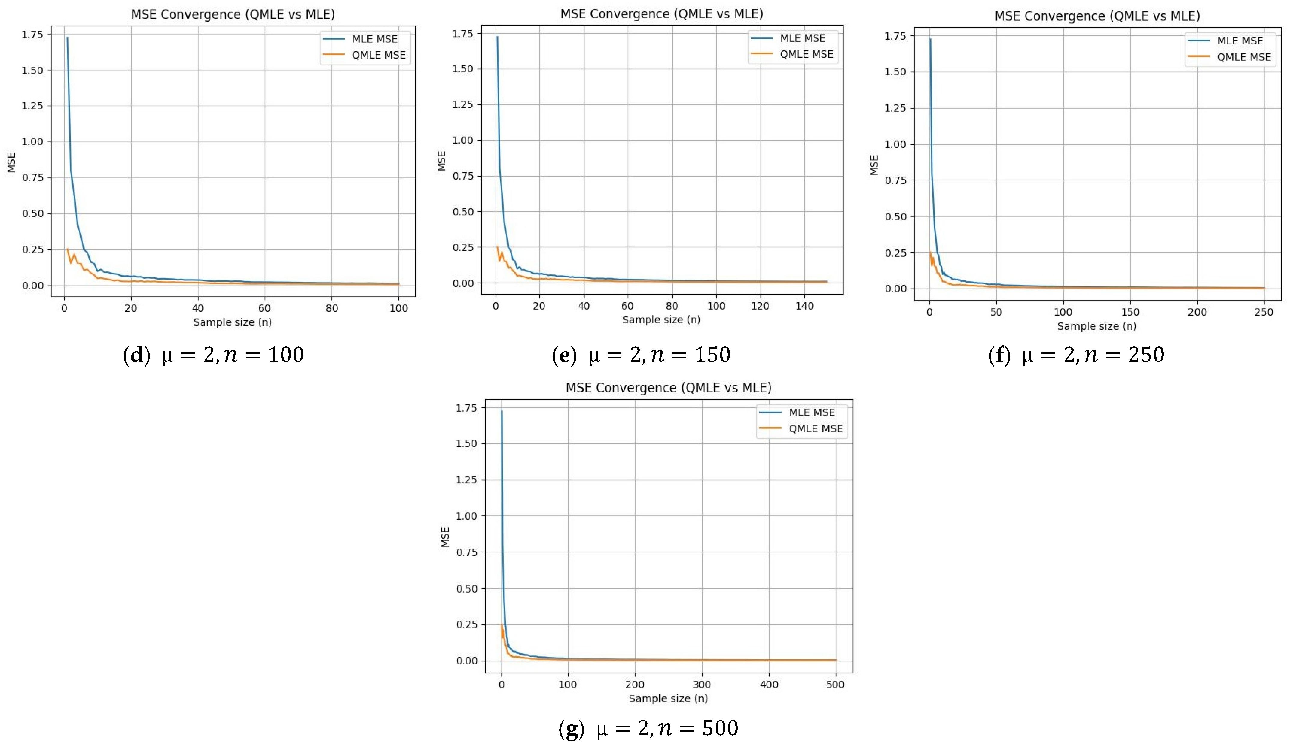
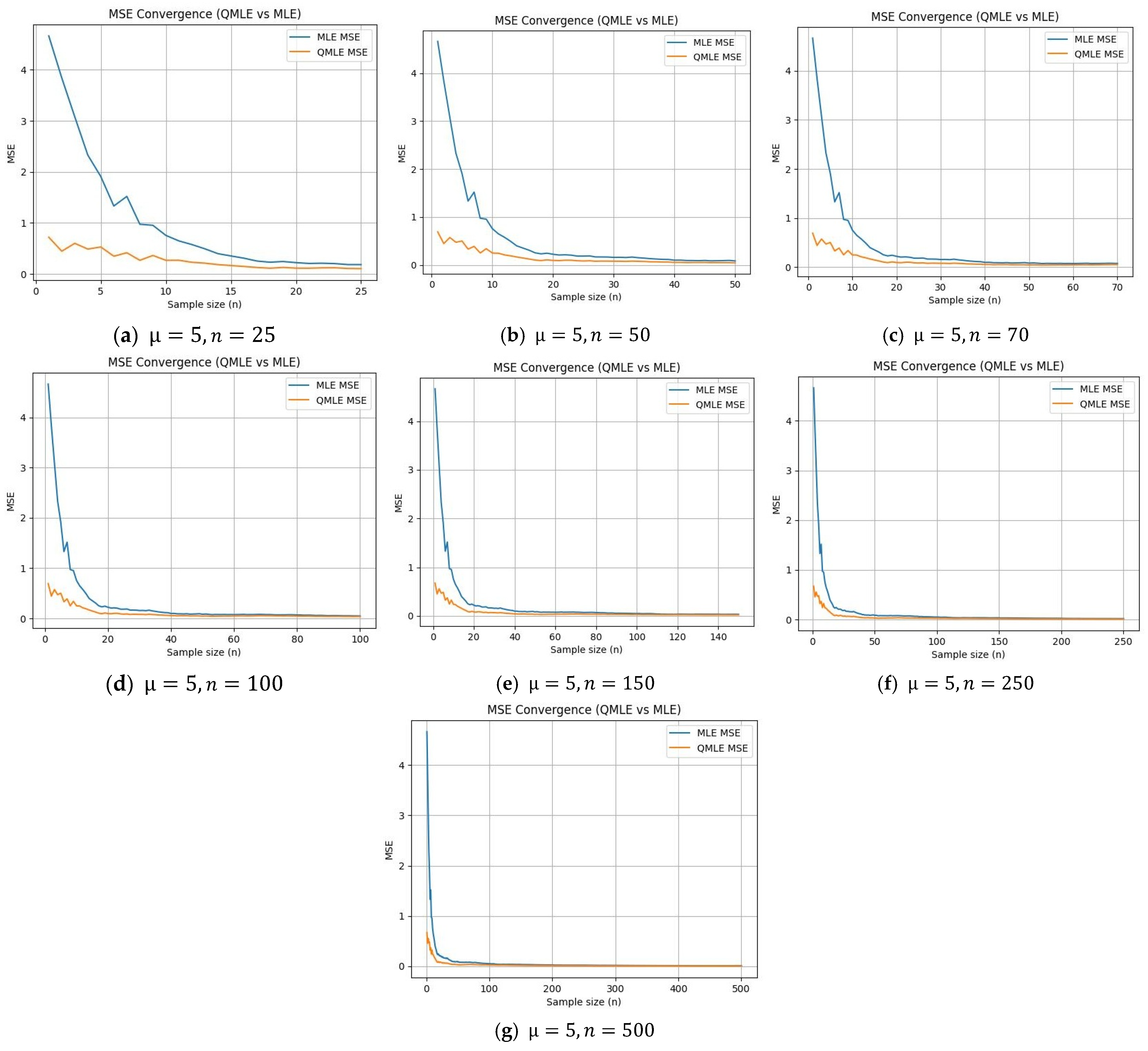
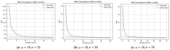
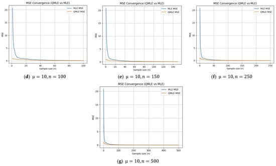
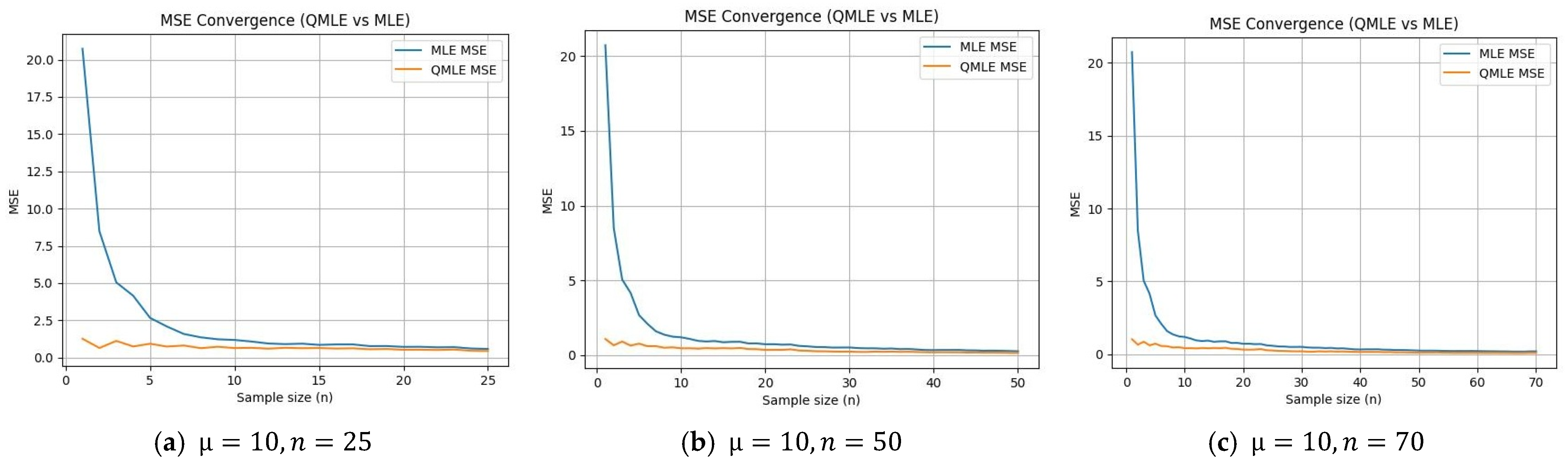
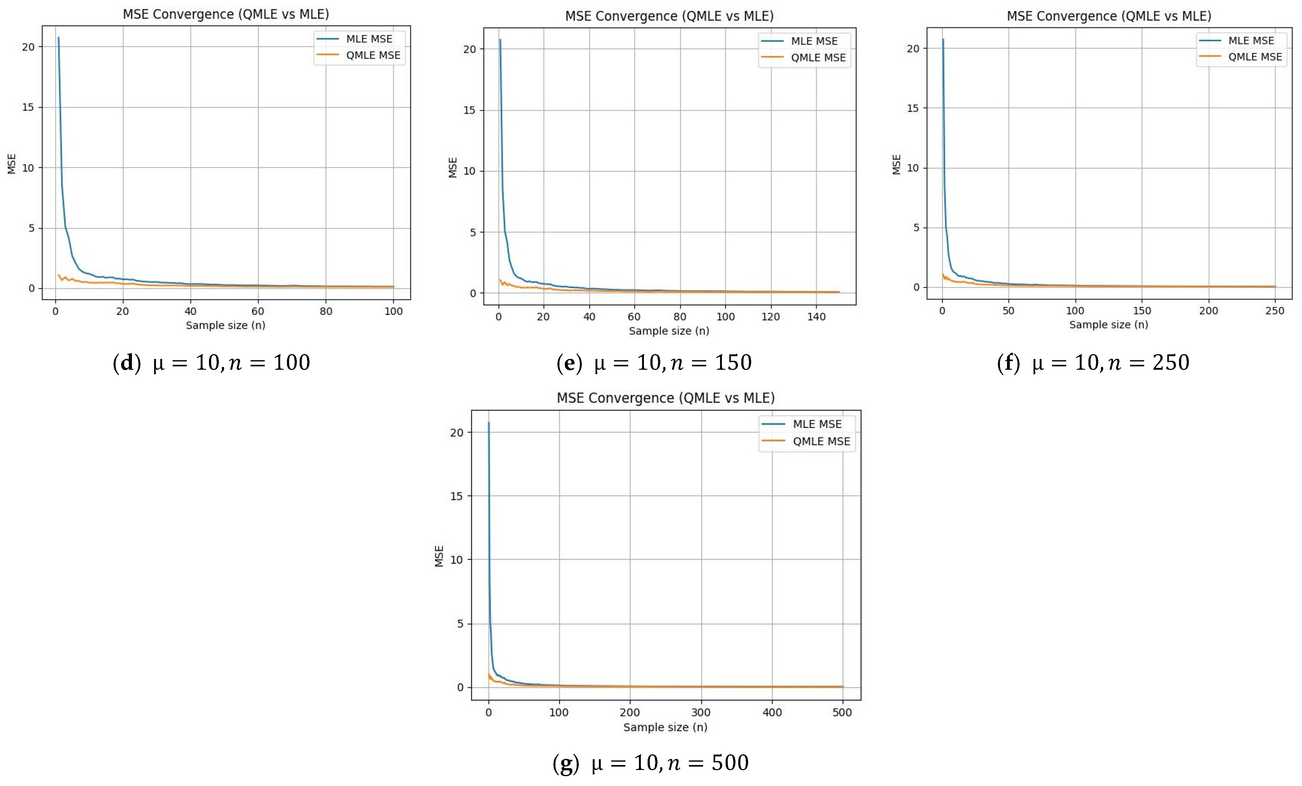
This study also performed a convergence analysis to evaluate the convergence of MLE and QMLE estimates towards the true parameter at each sample where and track the performance of both estimates as the sample sizes increase. This convergence analysis comprises the convergence toward the true parameter (Figure 3, Figure 4 and Figure 5), convergence rates (Figure 6, Figure 7 and Figure 8) and MSE convergence (Figure 9, Figure 10 and Figure 11). These figures indicate that QMLE estimates are closer to the true parameter than MLE estimates. Moreover, QMLE has a lower average absolute error than MLE, highlighting its superiority. All these findings indicate that QMLE outperforms the classical MLE method across numerous statistical metrics. These results validate that QMLE has the potential to be superior as a parameter estimation method.
Figure 3.
Convergence of MLE and QMLE estimates .
Figure 4.
Convergence of MLE and QMLE estimates .
Figure 5.
Convergence of MLE and QMLE estimates .
Figure 6.
Convergence Rate: QMLE vs. MLE .
Figure 7.
Convergence Rate: QMLE vs. MLE .
Figure 8.
Convergence Rate: QMLE vs. MLE .
Figure 9.
Convergence Curve: QMLE vs. MLE .
Figure 10.
Convergence Curve: QMLE vs. MLE .
Figure 11.
Convergence Curve: QMLE vs. MLE .
The robustness of our proposed QMLE framework is also evaluated by examining the sensitivity of the proposed method with respect to hyperparameters () and repeated MC runs. The results show that QMLE estimates are consistent and stable across all experiments and indicate robustness. We used Python (version 3.13.7) to perform simulations on the operating system of Microsoft Windows 11. NumPy (version 2.3.2) and SciPy (version 1.16.1) carried out the numerical computations, Matplotlib (version 3.10.5) provided visualizations.
7. Real-Data Applications
This section evaluates the performance of the QMLE approach in real-data applications. Four real-life datasets are used in this study to validate the potential computational advantages of QMLE over classical MLE. First, we source a publicly available dataset of “Human Body Temperature” comprising 130 measurements of body temperature (in Fahrenheit), gender and heart rate (beats per minute) from Kaggle provided by Devronic [30]. Temperature is the variable of interest in this study. The second dataset, comprising 100 breaking strengths of yarn, was originally presented by Duncan in 1974. Puig and Stephens [5] used and reported this dataset in their research. Third, a dataset of 33 observations comprising differences in flood levels between river stations is used. This is also used by Puig and Stephens and is available in their study [5]. Further, a dataset of failure times for 37 failed units in a life test is taken from a research article by Jan and Ahmad [4]. All these datasets were reported to follow the Laplace distribution. However, we also applied the Kolmogorov–Smirnov (K-S) test to confirm whether these datasets are consistent with the Laplace distribution or not, and the K-S test empirically validated it. All datasets are well-structured and valid for comparing the efficiency, accuracy, and robustness of the QMLE method for estimating the location parameter of the Laplace distribution with MLE. QMLE and MLE estimates of the location parameter are computed for all four datasets and reported in Table 4, where the MLE estimate is computed by taking the sample median of each dataset. Moreover, the SE and AL are calculated for both estimates and are presented in Table 4 to compare the performance of the estimation methods.
Table 4.
QMLE and MLE estimates of Laplace location parameter for real datasets.
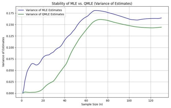
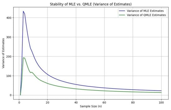
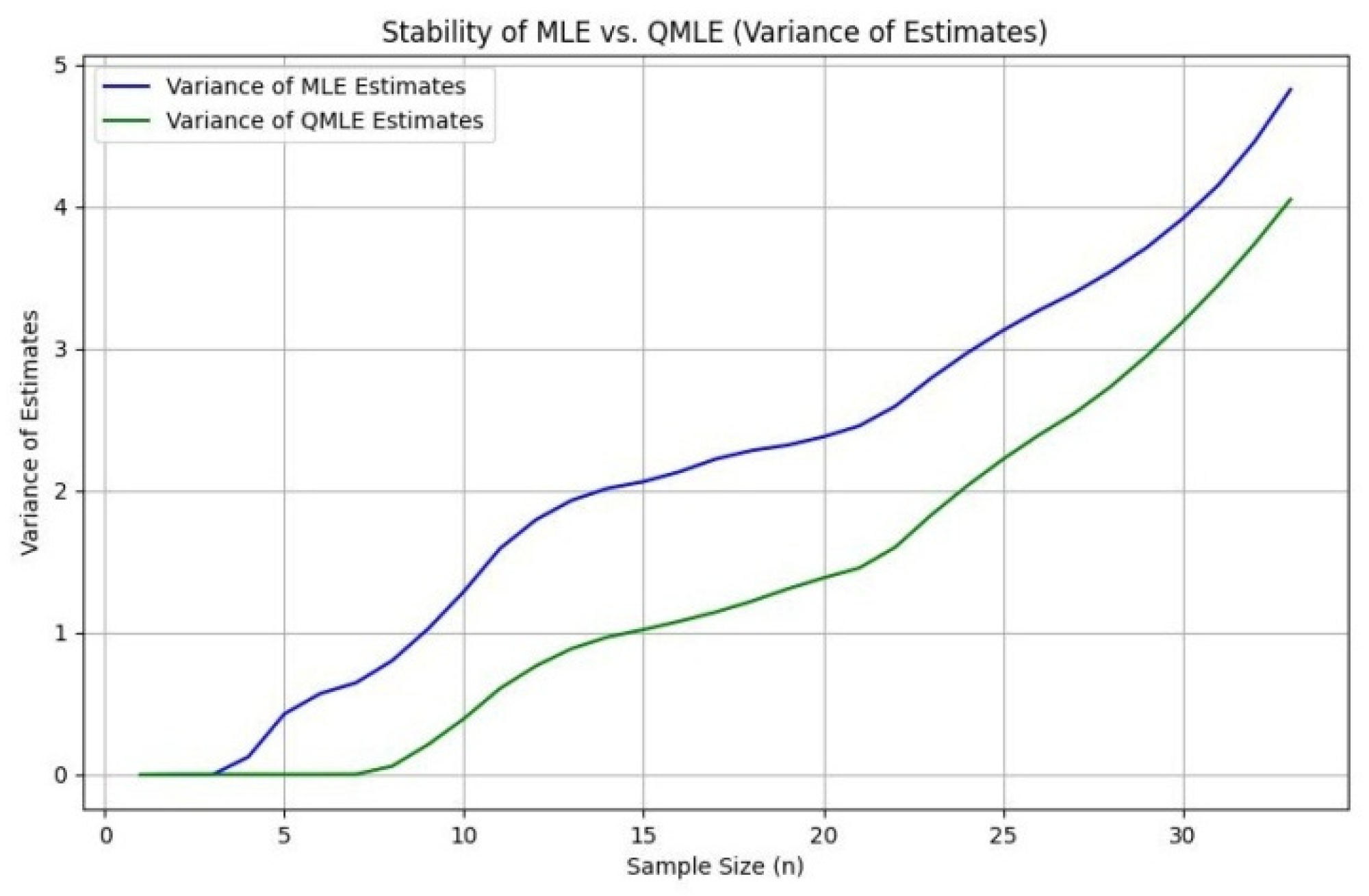
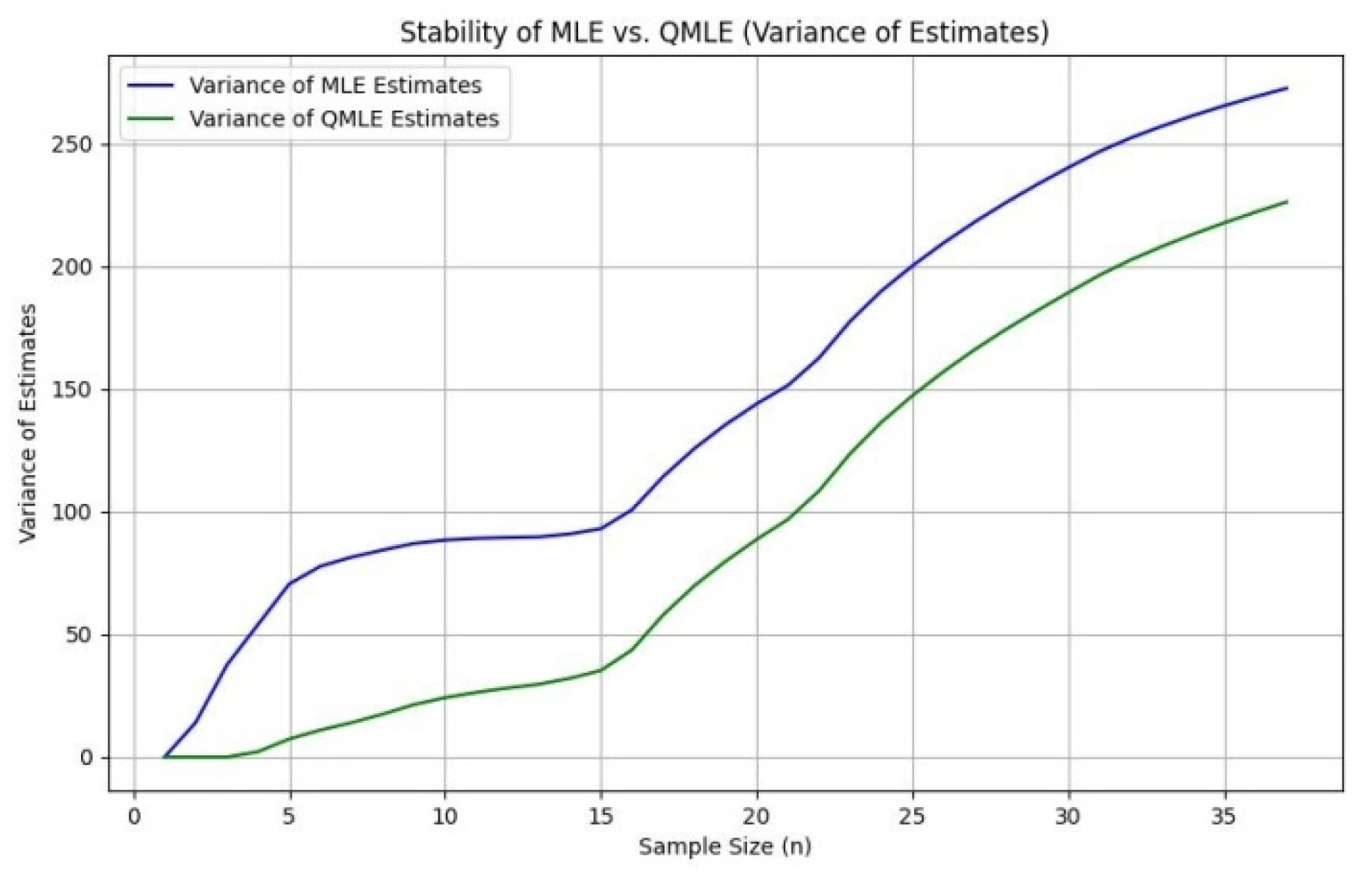
The results described above indicate that both methods provide closer estimates across all datasets, demonstrating the reliability of both methods. However, QMLE provides lower SE and AL values, with narrower CIs, compared to MLE estimates across all datasets. This suggests stronger statistical evidence that the QMLE is a more precise estimate and less uncertain around the true value of the parameter. The validity of the QMLE estimate is also evaluated through variance analysis at each sample where for all datasets. QMLE outperforms the classical MLE, achieving lower variances across all samples (see Figure 12, Figure 13, Figure 14 and Figure 15). The average variances and average efficiency are also computed for all datasets, and the results are reported in Table 4. The average variances of QMLE estimates are smaller than MLE estimates and indicate QMLE’s advantage over MLE in terms of efficiency and stability.
Figure 12.
Stability of MLE and QMLE estimates (temperature).
Figure 13.
Stability of MLE and QMLE estimates (breaking strength).
Figure 14.
Stability of MLE and QMLE estimates (flood levels).
Figure 15.
Stability of MLE and QMLE estimates (failure times).
All the findings validate the potential advantages of QMLE as a competitive and promising method for parameter estimation of the Laplace parameter. QMLE provides more accurate, precise, efficient, less uncertain, and better-fitting estimates than MLE when the true parameters are unknown and the estimator’s stability is important. Overall, the results indicate that statistical estimation theory can be improved by incorporating quantum dynamics into the classical estimation process.
8. Limitations and Future Directions
In the QMLE framework, evolution of quantum state and equation updates are involved. These additional steps performed on classical hardware increase some computational runtimes by a fixed amount. Potential benefits of quantum-inspired algorithms are difficult to achieve on classical platforms. Notwithstanding the developments in quantum hardware, it is facing some challenges and is not available yet on a large scale. Research may focus on the development of quantum algorithms until its availability on the required scale. The QMLE method is expected to achieve practical advantages of efficiency and runtime for statistical inference, outperforming the classical method of estimation as quantum hardware platforms mature.
The focus of the study is to establish the QMLE framework and validate the methodology for the estimation of location parameters of the Laplace distribution where the scale parameter is known. However, in future, this framework can be extended for the joint estimation of both parameters. Moreover, this study focuses on algorithm development and validates it empirically as an initial step to establish the effectiveness and feasibility of our proposed framework. However, future research is open for the theoretical derivations of statistical properties (consistency, asymptotic normality) of the QMLE framework.
9. Conclusions
In the present study, we incorporate quantum dynamics into the statistical estimation method, and a quantum-based estimation approach, i.e., quantum maximum likelihood estimation (QMLE), is proposed. The proposed QMLE method leverages quantum principles via the Kraus map, quantum states, sensitivity equations, and a quantum filter to estimate the unknown parameters of probability distributions. Further, this study implemented the QMLE method to estimate the Laplace location parameter. The Laplace distribution is important and is often used as an alternative to the Gaussian distribution in robustness studies. Parameter estimation plays a significant role in statistical inference, and accurate estimation of Laplace parameters is crucial in the fields of astronomy, life testing, medicine, environmental and biological sciences, inventory management, finance, and quality control. Classical estimation methods have some computational limitations for complex models and high-dimensional data. This study evaluates the performance of the QMLE estimate of the Laplace location parameter and compares with its MLE estimate in both simulation studies and real-world analyses. For this purpose, various statistical metrics such as bias, MAE, RME, AL, CP, RME, MSE, SE, variance, and CI are computed. The validity of the QMLE estimate is also evaluated through variance and convergence analyses. All the findings validate the potential computational advantages of the QMLE approach as a competitive and promising method for parameter estimation of the Laplace parameter. QMLE provides more accurate, precise, efficient, less uncertain, and better-fitting estimates than MLE. Overall, the results indicate that statistical estimation theory can be improved by incorporating quantum dynamics into the classical estimation process. This framework has the potential to pave the way for future research by extending it to other discrete and continuous distributions and by developing further methodologies for next-generation statistical inference and data science.
Author Contributions
Conceptualization, R.A.K.S.; methodology, A.R.; software, A.R.; validation, R.A.K.S., and A.R.; formal analysis, A.R.; investigation, A.R.; resources, A.R.; data curation, A.R.; writing—original draft preparation, A.R.; writing—review and editing, R.A.K.S.; visualization, A.R.; supervision, R.A.K.S.; project administration, R.A.K.S., funding acquisition, A.R. All authors have read and agreed to the published version of the manuscript.
Funding
This research received no external funding.
Data Availability Statement
The data sources used in the manuscript are cited and publicly available. Moreover, this research is part of the first author’s doctoral research, and the codes are confidential. The codes will be available to the editor/reviewers for verification purposes only.
Acknowledgments
The authors have reviewed and edited the output and take full responsibility for the content of this publication.
Conflicts of Interest
The authors have no conflicts of interest.
References
- Kotz, S.; Kozubowski, T.; Podgorski, K. The Laplace Distribution and Generalizations: A Revisit with Applications to Communications, Economics, Engineering, and Finance; Springer Science & Business Media: New York, NY, USA, 2001. [Google Scholar] [CrossRef] [Scilit]
- Chattamvelli, R.; Shanmugam, R. Laplace Distribution Continuous Distributions in Engineering and the Applied Sciences–Part II; Springer Nature: Cham, Switzerland, 2021; pp. 189–199. [Google Scholar] [CrossRef] [Scilit]
- Aryal, G.R. Study of Laplace and Related Probability Distributions and Their Applications. Ph.D. Thesis, University of South Florida, Tampa, FL, USA, 2006. [Google Scholar]
- Jan, U.; Ahmad, S. Bayesian Approximation Techniques for Scale Parameter of Laplace Distribution. J. Mod. Appl. Stat. Methods 2019, 17, 10. [Google Scholar] [CrossRef] [Scilit]
- Puig, P.; Stephens, M.A. Tests of fit for the Laplace distribution, with applications. Technometrics 2000, 42, 417–424. [Google Scholar] [CrossRef]
- Nadarajah, S. Reliability for Laplace distributions. Math. Probl. Eng. 2004, 2004, 169–183. [Google Scholar] [CrossRef] [Scilit]
- Ribeiro-Reis, L.D. Laplace distribution: Properties, regression model and simulation. J. Stat. Manag. Syst. 2022, 25, 489–499. [Google Scholar] [CrossRef] [Scilit]
- Mood, A.M. Introduction to the Theory of Statistics; McGraw-Hill Publishing Co., Ltd.: New York, NY, USA, 1950. [Google Scholar]
- Sun, W.; Zhu, X.; Zhang, Z.; Balakrishnan, N. Bayesian inference for Laplace distribution based on complete and censored samples with illustrations. J. Appl. Stat. 2025, 52, 914–935. [Google Scholar] [CrossRef] [Scilit] [PubMed]
- Hosking, J.R. L-moments: Analysis and estimation of distributions using linear combinations of order statistics. J. R. Stat. Soc. Ser. B Stat. Methodol. 1990, 52, 105–124. [Google Scholar] [CrossRef] [Scilit]
- Abdul Moniem, I.B. L-moments and TL-moments estimation for the exponential distribution. Far East J. Theor. Stat. 2007, 23, 51–61. [Google Scholar]
- Huber, P.J.; Ronchetti, E.M. Robust Statistics; John Wiley & Sons: Hoboken, NJ, USA, 2009. [Google Scholar]
- Adjieteh, M.; Brazauskas, V. Quantile least squares: A flexible approach for robust estimation and validation of location-scale families. Stat. Comput. 2025, 35, 106. [Google Scholar] [CrossRef] [Scilit]
- Baron, M. Probability and Statistics for Computer Scientists; Chapman and Hall/CRC: New York, NY, USA, 2019. [Google Scholar] [CrossRef] [Scilit]
- Hsu, H.P. Theory and Problems of Probability, Random Variables, and Random Processes; McGraw-Hill: New York, NY, USA, 1996; Volume 83. [Google Scholar]
- Hogg, R.V.; McKean, J.W.; Craig, A.T. Introduction to Mathematical Statistics; Pearson Education: Boston, MA, USA, 2019. [Google Scholar]
- Wasserman, L. All of Statistics: A Concise Course in Statistical Inference; Springer Science & Business Media: New York, NY, USA, 2013. [Google Scholar]
- Meeker, W.Q.; Escobar, L.A.; Pascual, F.G. Statistical Methods for Reliability Data; John Wiley & Sons: Hoboken, NJ, USA, 2021. [Google Scholar]
- Ali, S.; Aslam, M.; Abbas, N.; Kazmi, S.M.A. Scale parameter estimation of the Laplace model using different asymmetric loss functions. Int. J. Stat. Probab. 2012, 1, 105. [Google Scholar] [CrossRef] [Scilit]
- Nielsen, M.A.; Chuang, I.L. Quantum Computation and Quantum Information; Cambridge University Press: Cambridge, UK, 2010. [Google Scholar]
- Petz, D. Quantum Information Theory and Quantum Statistics; Springer Science & Business Media: Berlin/Heidelberg, Germany, 2007. [Google Scholar]
- Zohuri, B.; Rahmani, F.M. What is quantum computing and how it works. J. Mater. Sci. Manuf. Res. 2020, 3, 1–5. [Google Scholar] [CrossRef] [Scilit]
- Jozsa, R.; Linden, N. On the role of entanglement in quantum-computational speed-up. Proc. R. Soc. London. Ser. A Math. Phys. Eng. Sci. 2003, 459, 2011–2032. [Google Scholar] [CrossRef] [Scilit]
- Feynman, R.P. Feynman Lectures on Computation; CRC Press: Boca Raton, FL, USA, 2018. [Google Scholar]
- Clausen, H.G.; Rouchon, P.; Wisniewski, R. Online parameter estimation for continuously monitored quantum systems. IEEE Control Syst. Lett. 2024, 8, 1247–1252. [Google Scholar] [CrossRef] [Scilit]
- Cortez, L.; Chantasri, A.; García-Pintos, L.P.; Dressel, J.; Jordan, A.N. Rapid estimation of drifting parameters in continuously measured quantum systems. Phys. Rev. A 2017, 95, 012314. [Google Scholar] [CrossRef] [Scilit]
- Surace, S.C.; Pfister, J.-P. Online maximum-likelihood estimation of the parameters of partially observed diffusion processes. IEEE Trans. Autom. Control 2018, 64, 2814–2829. [Google Scholar] [CrossRef] [Scilit]
- Zhao, T.-L.; Hu, S.-X.; Zhang, Y. Maximum-likelihood-estimate Hamiltonian learning via efficient and robust quantum likelihood gradient. Phys. Rev. Res. 2023, 5, 023136. [Google Scholar] [CrossRef]
- Bouten, L.; Van Handel, R.; James, M.R. An introduction to quantum filtering. SIAM J. Control Optim. 2007, 46, 2199–2241. [Google Scholar] [CrossRef] [Scilit]
- Devronic. Human Body Temperature. Available online: https://www.kaggle.com/datasets/devronic/human-body-temperature (accessed on 25 November 2025).

Disclaimer/Publisher’s Note: The statements, opinions and data contained in all publications are solely those of the individual author(s) and contributor(s) and not of MDPI and/or the editor(s). MDPI and/or the editor(s) disclaim responsibility for any injury to people or property resulting from any ideas, methods, instructions or products referred to in the content. |
© 2026 by the authors. Licensee MDPI, Basel, Switzerland. This article is an open access article distributed under the terms and conditions of the Creative Commons Attribution (CC BY) license.